Jeffreys-prior penalty for high-dimensional logistic regression: A conjecture about aggregate bias

Abstract

Firth (1993, Biometrika) shows that the maximum Jeffreys’ prior penalized likelihood estimator in logistic regression has asymptotic bias decreasing with the square of the number of observations when the number of parameters is fixed, which is an order faster than the typical rate from maximum likelihood. The widespread use of that estimator in applied work is supported by the results in Kosmidis and Firth (2021, Biometrika), who show that it takes finite values, even in cases where the maximum likelihood estimate does not exist. Kosmidis and Firth (2021, Biometrika) also provide empirical evidence that the estimator has good bias properties in high-dimensional settings where the number of parameters grows asymptotically linearly but slower than the number of observations. We design and carry out a large-scale computer experiment covering a wide range of such high-dimensional settings and produce strong empirical evidence for a simple rescaling of the maximum Jeffreys’ prior penalized likelihood estimator that delivers high accuracy in signal recovery in the presence of an intercept parameter. The rescaled estimator is effective even in cases where estimates from maximum likelihood and other recently proposed corrective methods based on approximate message passing do not exist.

Keywords: mean bias reduction, approximate message passing, data separation

1 Introduction

1.1 Logistic regression with $p/n\to\kappa\in(0,1)$

Suppose we observe binary responses $y_{1},\ldots,y_{n}$ with $y_{i}\in\{0,1\}$, and $n$ vectors of covariates $x_{1},\ldots,x_{n}$ with $x_{i}\in\Re^{p}$. Consider a logistic regression model where $y_{1},\ldots,y_{n}$ are assumed to be realizations of independent Bernoulli random variables $Y_{1},\ldots,Y_{n}$, respectively, where $Y_{i}\mid x_{i}$ has expectation $\mu_{i}$ with

$$\log\frac{\mu_{i}}{1-\mu_{i}}=\eta_{i}=\beta_{0}+x_{i}^{\top}\beta\,,$$ (1)

with $\beta_{0}\in\Re$ and $\beta\in\Re^{p}$.

Under the assumptions that $p/n\to\kappa\in(0,1)$, $x_{1},\ldots,x_{n}$ are generated independently from a Normal distribution with mean $0_{p}$ and unknown, non-singular variance-covariance matrix $\Sigma$, and the signal strength is ${\mathop{\rm var}}(x_{i}^{\top}\beta)\to\gamma_{0}^{2}\in(0,\infty)$, Candès and Sur (2020) prove the existence of a phase transition curve on the plane of $\kappa$ and $\gamma=\sqrt{\beta_{0}^{2}+\gamma_{0}^{2}}$ that characterizes when the maximum likelihood (ML) estimate exists with probability approaching one as $n,p\to\infty$. That phase transition is found to be sharp for finite values of $n$ and $p$. By existence we mean that all the component of the ML estimate are finite, and we say that the ML estimate does not exist if at least one of its components is infinite.

Candès and Sur (2020, Theorem 2.1) shows that the phase transition curve can be computed efficiently for any given $\beta_{0}$ by minimizing a function of two unknowns over a grid of values for $\gamma$. This is in stark contrast to the usual route of detecting infinite estimates in logistic regression, which requires the solution of appropriate linear programs which operate only on a given set of responses and covariates, ignoring any knowledge of the distribution of the covariates. Such linear programs appear for example, in the seminal work of Albert and Anderson (1984), where data separation is a necessary and sufficient condition for the existence of the ML estimate. Konis (2007) provides an alternative linear program, which is implemented in the detectseparation R package (Kosmidis et al., 2022). Solving those linear programs, though, can be computationally demanding for large $n$ or $p$.

The phase transition curve is particularly useful because it identifies the ($\kappa$, $\gamma$) combinations for which the corrective methods of Sur and Candès (2019) and Zhao et al. (2022) apply for recovering consistency of the ML estimator and correcting inference from likelihood-based pivots in the high-dimensional logistic regression with $p/n\to\kappa\in(0,1)$. Specifically for estimation, approximate message passing arguments are used to derive a system of nonlinear equations in Sur and Candès (2019, expression (5)), whose solution provides the factor by which the ML estimator needs to be re-scaled in order to correct its persistent bias and recover aggregate unbiasedness. As Sur and Candès (2019) clearly note, that system of equations does not have a unique solution if $(\kappa,\gamma)$ are on the side of the phase transition curve where the ML estimate does not exist asymptotically, and the corrective approaches they introduce do not apply.

1.2 Logistic regression with fixed $p$ and $n\to\infty$

Firth (1993) shows that for logistic regression with fixed $p$ and $n\to\infty$, the estimator of $\theta=(\beta_{0},\beta^{\top})^{\top}$ that results by the maximization of the Jeffreys’ prior penalized log-likelihood

$$\tilde{\ell}(\theta)=\ell(\theta)+\frac{1}{2}\log\left|X^{\top}W(\theta)X\right|$$ (2)

has bias of order $O(n^{-2})$, which is asymptotically smaller than the $O(n^{-1})$ bias that is expected by the ML estimator from standard asymptotic theory (see, for example, McCullagh, 1987, Section 7.3). We say “generally” here because, formally, the bias of the ML estimator conditional on the observed covariates is not defined for a logistic regression model, as there is always at least one configuration of responses which results in ML estimates with infinite components. In (2), $\ell(\theta)=\sum_{i=1}^{n}\{y_{i}\eta_{i}-\log(1+\exp{\eta_{i}})\}$ is the log-likelihood of the logistic regression model with linear predictor $\eta_{i}$ as in (1), $X$ is the $n\times p$ model matrix with $x_{1},\ldots,x_{n}$ in its rows, and $W(\theta)$ is a diagonal matrix with $i$th diagonal element $\mu_{i}(1-\mu_{i})$. Importantly, Kosmidis and Firth (2021) show that the maximum Jeffreys’ prior penalized likelihood (mJPL) estimator has always finite components, even in cases where the ML estimate does not exist, under the sole assumption that $X$ is of full rank. Those results underpin the increasingly widespread use of mJPL and similarly penalized likelihood estimation in logistic regression models in many applied fields. For example, at the date of writing Firth (1993) has about $4500$ citations in Google Scholar, across areas of scientific enquiry, with the majority being due to the properties of mJPL in logistic regression.

Both Sur and Candès (2019) and Kosmidis and Firth (2021) also present empirical evidence that mJPL appears to deliver a substantial reduction in the persistent bias of the ML estimator in high-dimensional logistic regression setting of Section 1.1, whenever the ML estimate exists. We should note here that, as is the case for ML estimation, the mJPL estimates can be computed efficiently through a range of methods, the most popular ones being iterative reweighted least squares Kosmidis et al. (see 2020, for details) or repeated maximum likelihood fits on adaptively adjusted responses (see Kosmidis and Firth, 2021, Section 4). R packages such as brglm2 (Kosmidis, 2023) and logistf (Heinze et al., 2023) provide efficient implementations.

1.3 Contribution

We design and carry out a large-scale computer experiment to examine in depth and expand the observations of Sur and Candès (2019) and Kosmidis and Firth (2021).

The results we gather provide further evidence that mJPL performs well and markedly better than the ML estimator in the region below Candès and Sur (2020)’s phase transition curve where the ML estimate asymptotically exists, and tends to over-correct in the region where the ML estimate has infinite components. A careful statistical analysis of the results allows us to confidently state that the amount of over-correction can be accurately characterized in terms of $\kappa$, $\gamma$ and the relative size of the intercept parameter $\beta_{0}$ and $\gamma_{0}$, for a wide range of $(\kappa,\gamma)$ values. As a result, we are able to formulate and contribute a fruitful conjecture about adjusting the mJPL estimates post-fit to almost recover the true signal to high accuracy and for a wide range of settings. We should emphasize that the conjecture also applies in the region above Candès and Sur (2020)’s phase transition curve, where the ML estimate does not exist with probability approaching one, and the methods of Sur and Candès (2019) and Zhao et al. (2022) do not apply.

Conjecture 1.1:

Consider the logistic regression model (1) where $x_{1},\ldots,x_{n}$ are realizations of $n$ independent $N_{p}(0,\Sigma)$ random vectors, and assume that $p/n\to\kappa\in(0,1)$ and $\beta$ is such that ${\mathop{\rm var}}(x_{i}^{\top}\beta)\to\gamma_{0}^{2}$, as $n,p\to\infty$. Then, the mJPL estimator $(\tilde{\beta}_{0},\tilde{\beta}^{\top})^{\top}$ from the maximization of (2) satisfies

$$\frac{1}{p}\sum_{j=1}^{p}(\tilde{\beta}_{j}-\alpha_{\star}\beta_{j})\overset{p}{\to}0\,,$$ (3)

with $\alpha_{\star}\leq 1$. For small to moderate values of $\beta_{0}^{2}/\gamma_{0}^{2}$, the scaling $\alpha_{\star}$ can be approximated by

$$q(\kappa,\gamma,\gamma_{0};b)=\left\{\begin{array}[]{ll}1\,,&\text{if }\kappa<h_{\rm MLE}(\beta_{0},\gamma_{0})\\ \kappa^{b_{1}}\gamma^{b_{2}}\gamma_{0}^{b_{3}}\,,&\text{if }\kappa>h_{\rm MLE}(\beta_{0},\gamma_{0})\end{array}\right.\,,$$

where $b_{1}<-1$, $b_{2}<-1$, $b_{3}>0$. The function $h_{\rm MLE}(\beta_{0},\gamma_{0})$ is as defined in Candès and Sur (2020, Theorem 2.1), which states that the ML estimate exists with probability approaching one if $\kappa<h_{\rm MLE}(\beta_{0},\gamma_{0})$, and zero if $\kappa>h_{\rm MLE}(\beta_{0},\gamma_{0})$.

Statement (3) is what we refer to as aggregate bias, and the parameters $\alpha_{\star}$ and $q(\kappa,\gamma,\gamma_{0};b)$ are the aggregate bias parameter, and its approximation, respectively. Equivalently, the conjecture implies that rescaling $\tilde{\beta}_{j}$ to $\tilde{\beta}_{j}/q(\kappa,\gamma,\gamma_{0};b)$ produces an estimator that has almost zero aggregate bias for small to moderate values of $\beta_{0}^{2}/\gamma_{0}^{2}$.

Our predictions for $b_{1}$, $b_{2}$, and $b_{3}$ are $-1.172$, $-1.869$, and $0.817$, respectively; see Table 1, which also provides $95\%$ bootstrap BC$\alpha$ confidence intervals for $b_{1}$, $b_{2}$, and $b_{3}$. We also have evidence that $\kappa^{b_{1}}\gamma^{b_{2}}\gamma_{0}^{b_{3}}<1$ when the ML estimate does not exist asymptotically (see, for example, top left of Figure 2).

To our knowledge, there has been no other tuning-parameter free proposal for signal recovery in the high-dimensional logistic regression setting of Sur and Candès (2019) and Zhao et al. (2022) with intercept parameter, which applies regardless of whether the ML estimate exists or not and does not require approximate message passing machinery to operate. A proof of that conjecture, at least when there is no intercept parameter, may proceed by adapting the framework and results in Salehi et al. (2019) to the case where the likelihood is penalized by Jeffreys’ prior and examining whether the solution of the resulting system of nonlinear equations in Salehi et al. (2019, see, for example, expression (6)) is approximately equal to the scaling factor $q(\kappa,\gamma,\gamma_{0};b)$ for small to moderate values of $\beta_{0}^{2}/\gamma_{0}^{2}$.

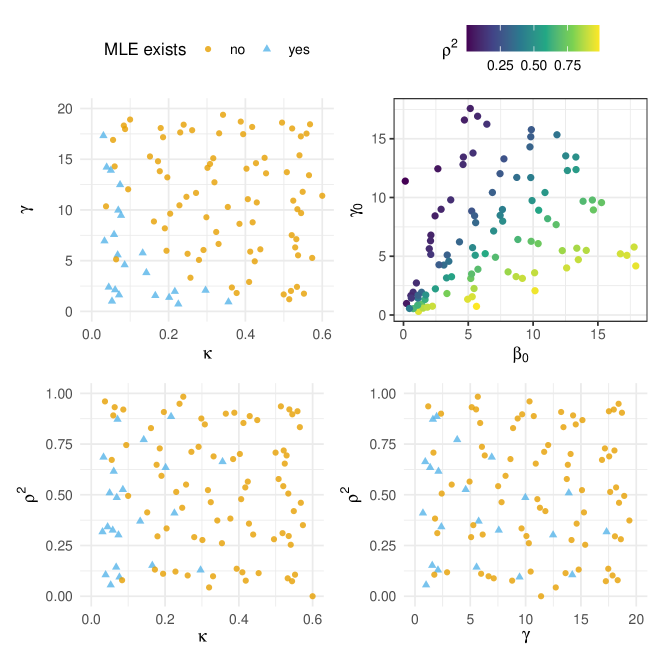
Figure 1: Top left, bottom left, and bottom right: $100$ points $(\kappa,\gamma,\rho^{2})\in(0,0.6)\times(0,20)\times(0,1)$ generated using a minimax projection design (Mak and Joseph, 2018), plotted on the three two-dimensional subspaces. At each point, Candès and Sur (2020, Theorem 2.1) is used to determine whether the ML estimate exists asymptotically or not. Top right: The implied $(\beta_{0},\gamma_{0})$ combinations.

The computer experiment also allows us to assess the performance of the implementation of mJPL provided by the well-used R package brglm2. brglm2 is more general than mJPL for logistic regression, providing also methods for mean and median bias reduction for all generalized linear models under a unifying interface and code base (see Kosmidis et al., 2020, for details), written exclusively in R. Hence, it provides a good benchmark relative to a purpose-built compiled program for mPJL for logistic regression that would naturally be much more efficient. It is found that, in notable contrast to the observations in Sur and Candès (2019, Supporting Information document, Section D), where mJPL is reported to be computationally infeasible in high-dimensional logistic regression settings, requiring about $2.5$ hours for $n=2000$ and $p=400$, the average runtime we observed for mJPL for $n=2000$ and $p$ ranging from $20$ to $1100$ is from milliseconds to under two minutes. See Section 5 for details.

2 Computer experiment

2.1 Data generating process

For generating a single data set from model (1), under the assumptions of Conjecture (1.1), we specify $n$, $\kappa\in(0,1)$, $\gamma_{0}>0$, $\gamma>0$, an initial parameter vector $\beta^{*}$, and set $p=\lceil n\kappa\rceil$. In order to control the relative size of the intercept parameter and $\gamma_{0}$, we define $\beta_{0}=\gamma\rho$, and $\gamma_{0}=\gamma\sqrt{1-\rho^{2}}$. In this way, $\beta_{0}^{2}/\gamma_{0}^{2}=\rho^{2}/(1-\rho^{2})$. This is the same relationship between $\beta_{0}$ and $\gamma_{0}$ that is used for producing Candès and Sur (2020, Figure 1(b)).

Conjecture 1.1 allows for correlated covariates as in Zhao et al. (2022). Hence, we also specify a $p\times p$, positive definite variance-covariance matrix $\Sigma$ for the covariates. We should mention here that, as noted in Zhao et al. (2022), the asymptotic framework of Candès and Sur (2020) is fully characterized by the values of the dimensionality constant $\kappa$, the limiting signal strength $\gamma_{0}$, and the size of the intercept parameter. The variance-covariance matrix $\Sigma$ of the covariate vectors, while necessary when simulating covariate vectors, can be arbitrary as long as ${\mathop{\rm var}}(x_{i}^{\top}\beta)\to\gamma_{0}^{2}$. We form an $n\times p$ matrix $X$ by generating its rows from $n$ independent and identically distributed normal random vectors with mean $0_{p}$ and variance-covariance matrix $\Sigma$ having $(i,j)$th element $\psi^{|i-j|}$, with $\psi\in(-1,1)$. We, then, re-scale $\beta^{*}$ to $\beta=\gamma_{0}\beta^{*}/\lVert L^{\top}\beta^{*}\rVert_{2}$, so that we control ${\mathop{\rm var}}(x_{i}^{\top}\beta)=\beta^{\top}LL^{\top}\beta=\gamma_{0}^{2}$, where $L$ is the Cholesky factor of $\Sigma$. Finally, we generate $y_{1},\ldots,y_{n}$ independently with $Y_{i}\sim\text{Bernoulli}(\mu_{i})$, where $\mu_{i}$ is specified in (1).

2.2 Training and test phases

The computer experiment has two phases. The first phase is a training phase and involves a specific simulation experiment using a space-filling design of $(\kappa,\gamma,\rho^{2})$ points, and $\psi=0$, that is the entries of $X$ are realizations of independent $N(0,1)$ random variables. The training phase is used to generate strong evidence for the approximation to $\alpha_{\star}$ in Conjecture 1.1 and predict the value of the constants $b_{1}$, $b_{2}$ and $b_{3}$. In the test phase, the generalizability of the prediction for the approximate form of $\alpha_{\star}$ is examined using independent simulation experiments for a preset grid of $(\kappa,\gamma,\rho^{2},\psi)$, which are different from the one used in the training phase. We produce strong evidence on the generality of the approximate form for $\alpha_{\star}$ in Conjecture 1.1.

3 Training phase

Table 1: Estimates and $95\%$ confidence intervals for the parameters of the linear regression of $\log\delta_{1}^{*}$ on $\log(\kappa)$, $\log(\gamma)$ and $\log(1-\rho^{2})$ for all design points with $\rho^{2}<0.7$. The confidence intervals are bootstrap $\mathop{\rm BC}_{\alpha}$ confidence intervals computed using $9999$ bootstrap samples through case resampling.

	Estimate	2.5 %	97.5 %
$b_{0}$	$-0.033$	$-0.137$	$0.069$
$b_{1}$	$-1.172$	$-1.211$	$-1.130$
$b_{2}$	$-1.869$	$-2.004$	$-1.730$
$b_{3}$	$0.817$	$0.689$	$0.942$
$\phi$	$0.004$

We compute a minimax projection design (Mak and Joseph, 2018) of $100$ points $(\kappa,\gamma,\rho^{2})\in(0,0.6)\times(0,20)\times(0,1)$ using the minimaxdesign R package (Mak, 2021). We choose the minimax projection design because, on one hand, it has the appealing property of uniform coverage of the design space in worst-case scenarios, and, on the other hand, improves on uniform coverage in projected subspaces of the design space; see Mak and Joseph (2018) for more details. Figure 1 shows the computed points on all two-dimensional subspaces. Candès and Sur (2020, Theorem 2.1) is used at each of the $100$ points to determine whether the ML estimate exists asymptotically or not. The ML estimate exists asymptotically at $22$ points.

We set $n=2000$ and $\psi=0$. Then, for each point on the minimax projection design, $\beta^{*}$ is set to an equi-spaced grid of length $p=\lceil n\kappa\rceil$ between $1$ and $10$, and $100$ samples of $X$ and $y$ are drawn independently as detailed in Section 2.1. The ML estimates of $\beta_{0}$ and $\beta$ are computed only in settings where the ML estimate asymptotically exists, and the mJPL estimates are computed everywhere using the brglm_fit() method for the glm() R function, as provided by the brglm2 R package. We compute the estimates so that they are accurate to the third decimal point and allowing up to $300$ of the quasi Fisher scoring iterations brglm_fit() implements; see the vignettes of Kosmidis (2023) for details on the quasi Fisher scoring iteration. The mJPL estimates are computed starting at zero for all parameters, and are used as starting values for the ML estimates, whenever the latter are computed.

Figure 2: Results from the training phase in Section 3. Top left: a scatterplot of $\log\delta_{1}^{*}$ versus $\log q(\kappa,\gamma,\gamma_{0};b^{*})$ for design points with $\rho^{2}\leq 0.7$ and design points with $\rho^{2}>0.7$, when the ML estimate does not exist asymptotically. The grey line is a $45^{o}$ reference line. Top right: scatterplot of the design points in Figure 1 for which the ML estimate exists. The points are coloured accourding to the value of $\log\delta_{1}^{*}$. Bottom: Histogram of $\log\delta_{1}^{*}$ across design points.

Evidence for Conjecture 1.1 is that, for all design points $(\kappa,\gamma,\rho^{2})$ (or equivalently $(\kappa,\gamma,\gamma_{0})$), the simple linear regression of the realizations of $\tilde{\beta}=(\tilde{\beta}_{1},\ldots,\tilde{\beta}_{p})^{\top}$ on the true values $\beta=(\beta_{1},\ldots,\beta_{p})^{\top}$ has intercept $\delta_{0}(\kappa,\gamma,\gamma_{0})=0$, and slope $\delta_{1}(\kappa,\gamma,\gamma_{0})=1$ if the ML estimate exists asymptotically, and $\delta_{1}(\kappa,\gamma,\gamma_{0})=\kappa^{b_{1}}\gamma^{b_{2}}\gamma_{0}^{b_{3}}$ if the ML estimate does not exist asymptotically.

For the case where the ML estimate does not exist, consider a multiplicative regression model with constant coefficient of variation (see McCullagh and Nelder, 1989, Chapter 8) where ${\mathop{\rm E}}(\delta_{1}^{*})=e^{b_{o}}\kappa^{b_{1}}\gamma^{b_{2}}\gamma_{0}^{b_{3}}$. Estimates for $b_{0}$, $b_{1}$, $b_{2}$ and $b_{3}$ can be computed using maximum likelihood for a Gamma-response generalized linear model with log link, which is formally equivalent to quasi-likelihood estimation (Wedderburn, 1974) with response variance $\phi\{{\mathop{\rm E}}(\delta_{1}^{*})\}^{2}$, where $\phi$ is a dispersion parameter. The dispersion parameter can be estimated after computing the estimates of $b$, using a moment-based estimator (see, for example, McCullagh and Nelder 1989, Section 8.3 and the summary.glm function in R). In support of Conjecture 1.1, it is straightforward to find moderate-valued thresholds $r\in(0,1)$ for $\rho^{2}$ (or equivalently for $\beta_{0}^{2}/\gamma_{0}^{2}$), for which a Gamma-response generalized linear model with log link is almost a perfect fit for all design points with $\rho^{2}\leq r$. For example, Table 1 shows estimates and 95% bootstrap confidence intervals for $b_{0}$, $b_{1}$, $b_{2}$ and $b_{3}$ based on the $70$ design points with $\rho^{2}\leq r=0.7$ ($\beta_{0}^{2}/\gamma_{0}^{2}\leq 7/3$). That fit is found to explain $99.34\%$ of the null deviance, and an inspection of the residuals reveals no evidence of departures from the assumptions of a multiplicative regression model with constant coefficient of variation. Under the Gamma regression model, ${\mathop{\rm E}}(\log\delta_{1}^{*})\simeq\log\mu-\phi/2$. Given the small value of the estimate of $\phi$, a linear regression of $\log\delta_{1}^{*}$ on $\log(\kappa)$, $\log(\gamma)$ and $\log(1-\rho^{2})$ should be an excellent fit, too, with almost identical estimates to those in Table 1. This is indeed the case; that linear regression returns estimates $-0.037$, $-1.171$, $-1.871$, and $0.822$ for $b_{0}$, $b_{1}$, $b_{2}$, and $b_{3}$, respectively, explaining $R^{2}=99.32\%$ of the variability in $\log\delta_{1}^{*}$.

The top left of Figure 2 shows a scatterplot of $\log\delta_{1}^{*}$ versus $\log q(\kappa,\gamma,\gamma_{0};b^{*})$ for design points with $\rho^{2}\leq 0.7$ and design points with $\rho^{2}>0.7$, where $b^{*}=(b_{1}^{*},b_{2}^{*},b_{3}^{*})^{\top}$ is the estimate of $(b_{1},b_{2},b_{3})^{\top}$ given in Table 1 (i.e. ignoring $b_{0}$, for which there is also no evidence that it is not zero). The points agree closely with the reference line of slope one through the origin when $\rho^{2}\leq 0.7$. That agreement starts progressively breaking down as $\rho^{2}$ grows, or, equivalently, as the relative size of the intercept $\beta_{0}$ to the signal strength $\gamma_{0}$ grows. Furthermore, $\kappa^{b_{1}^{*}}\gamma^{b_{2}^{*}}\gamma_{0}^{b_{3}^{*}}<1$, except from a few points that are close to phase transition.

At the top right of Figure 2 we see that the values of $\delta_{1}^{*}$ at the design points where the ML estimate exists asymptotically are about one (having a sample mean of $1.016$ and standard deviation of $0.0311$). This is strong evidence for the conjectured approximation to the aggregate bias parameter $\alpha_{\star}$ when the ML estimate exists. The finite sample distribution of $\delta_{1}^{*}$ for $n=2000$, when the ML estimate asymptotically exists, seems to be right-skewed (sample skewness is $1.483$), with larger values at points close to the phase transition for existence.

Finally, as is also apparent from the histogram on the bottom of Figure 2, the distribution of $\delta_{0}^{*}$ is concentrated around zero with minuscule variance.

4 Test phase

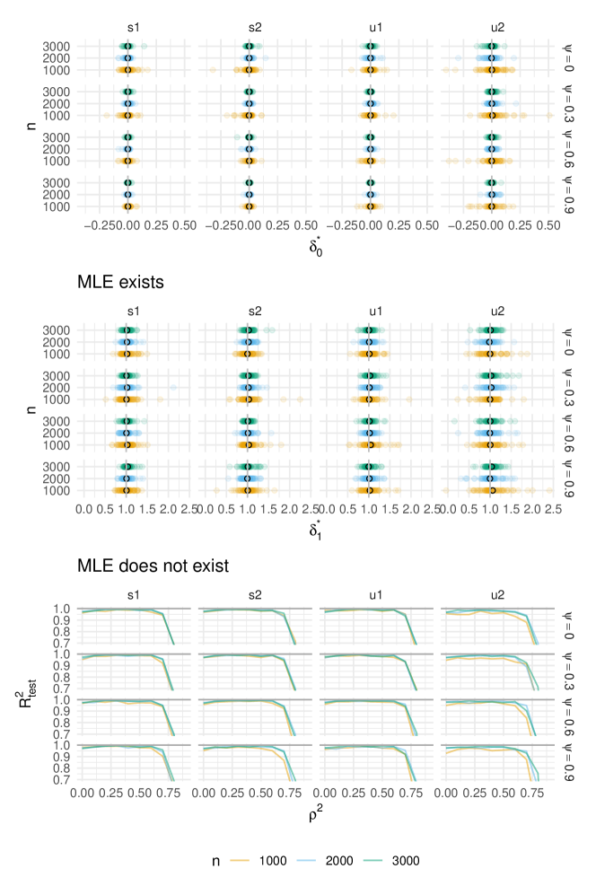
Figure 3: Results from the test phase in Section 4. Top and middle: Strip plots of the estimates $\delta_{0,{\rm test}}$, and $\delta_{1,{\rm test}}$ when the ML estimate exists asymptotically, respectively, for all combinations of $n$, $\psi$, and $\beta^{*}$ configuration. The black circles are the empirical averages of the values displayed in each strip plot. Bottom: $R^{2}_{\rm test}$, when the ML estimate does not exist asymptotically, as a function of $\rho^{2}$ for all combinations of $n$, $\psi$, and $\beta^{*}$ configuration.

We now test our prediction of the approximation to the aggregate bias parameter

$$q(\kappa,\gamma,\gamma_{0};b^{*})=\left\{\begin{array}[]{ll}1\,,&\text{if }\kappa<h_{\rm MLE}(\beta_{0},\gamma_{0})\\ \kappa^{b_{1}^{*}}\gamma^{b_{2}^{*}}\gamma_{0}^{b_{3}^{*}}\,,&\text{if }\kappa>h_{\rm MLE}(\beta_{0},\gamma_{0})\end{array}\right.\,,$$ (4)

developed in Section 3, using independent simulation experiments. We consider all possible combinations of $n\in\{1000,2000,3000\}$, $\psi\in\{0,0.3,0.6,0.9\}$, $\rho^{2}\in\{0,0.1,\ldots,0.9\}$, and the following four configurations for $\beta^{*}$:

• an equi-spaced grid of length $p$ between $-10$ and $10$;

• the first $\lceil p/5\rceil$ elements are $-10$, the second $\lceil p/5\rceil$ elements are $10$, and the remaining elements are zero;

• the first $\lceil p/5\rceil$ elements are $-3$, the second $\lceil p/5\rceil$ elements are -1, the last $\lceil p/5\rceil$ elements are 1, and all other elements are zero;

• an equi-spaced grid of length $p$ between $1$ and $10$, where $p=\lceil n\kappa\rceil$.

Configurations s1 and s2 are symmetric about zero, while u1 and u2 are not. For each of the $480$ combinations, we simulate one sample, as detailed in Section 2.1, at each of the $30$ $(\kappa,\gamma)$ points shown in the panels of Figure 4. We denote the set of those points as $D_{\rm test}$. Then, from each sample, we estimate the intercept $\delta_{0}$ and slope $\delta_{1}$ of the simple linear regression of the mJPL estimates on the corresponding true values.

The top and middle panels of Figure 3 show strip plots of the estimates $\delta_{0,{\rm test}}$ for all settings, and the estimates $\delta_{1,{\rm test}}$ when the ML estimate exists asymptotically, respectively, for all combinations of $n$, $\psi$, and $\beta^{*}$ configuration. As is evident, those estimates are concentrated around zero and one, respectively, in all test cases, with variance decreasing with $n$, exactly as we would expect under Conjecture 1.1. The quality of the predictions $q(\kappa,\gamma,\gamma_{0};b^{*})=\kappa^{b_{1}^{*}}\gamma^{b_{2}^{*}}\gamma_{0}^{b_{3}^{*}}$, with $b^{*}$ as in Table 1, for $\delta_{1,{\rm test}}$ when the ML estimate does not exist asymptotically can be assessed for each $\beta^{*}$ configuration, using the out-of-sample version of the coefficient of determination

$$R^{2}_{{\rm test}}(n,\rho^{2},\psi)=\frac{\sum\left\{\log\delta_{1,{\rm test}}-\log q(\kappa,\gamma,\gamma_{0};b^{*})\right\}^{2}}{\sum\left\{\log\delta_{1,{\rm test}}-\sum\log\delta_{1,{\rm test}}/30\right\}^{2}}\,.$$

All summations are over all $(\kappa,\gamma)\in D_{\rm test}$, and the dependence of $\delta_{1,{\rm test}}$ on $n$, $\psi$, $\kappa$, $\gamma$, and $\rho^{2}$ (or equivalently $\gamma_{0}$) is suppressed for notational convenience. The quantity $R^{2}_{{\rm test}}(n,\rho^{2},\psi)\in(-\infty,1]$, and a value of $1$ has the usual interpretation that the predicted values $\log q(\kappa,\gamma,\gamma_{0};b^{*})$ explain all the variability in $\log\delta_{1,{\rm test}}$. The bottom panel of Figure 3 shows the value of $R^{2}_{\rm test}$ as a function of $\rho^{2}$ for all combinations of $n$ and $\psi$ we consider. The approximation $q(\kappa,\gamma,\gamma_{0};b^{*})$ to the aggregate bias parameter $\alpha_{\star}$ is found to have excellent out-of-sample performance for small to moderate values of $\rho^{2}$, as we would expect if Conjecture 1.1 holds.

Figure 4 shows the mJPL estimates and their rescaled versions after division by $q(\kappa,\gamma,\gamma_{0};b^{*})$, for $n=3000$, $\psi=0.3$, $\rho^{2}=0.6$, and $\beta^{*}$ configuration u1, and Figure 5, for $n=1000$, $\psi=0.6$, $\rho^{2}=0.1$, and $\beta^{*}$ configuration s1, with one sample per $(\kappa,\gamma)$ point. The rescaled mJPL estimator results in excellent signal recovery.

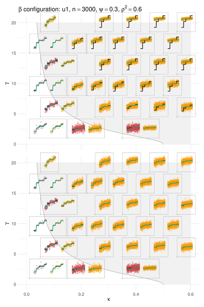
Figure 4: mJPL estimates (top) and their rescaled versions after division by (4) (bottom) for $n=3000$, $\psi=0.3$, $\rho^{2}=0.6$, and $\beta^{*}$ configuration u1 versus the parameter index, with one sample per $(\kappa,\gamma)$ point. The ML estimate exists asymptotically in the white area and does not exist asymptotically in the grey area. The blue segments show the sample mean of the estimates for each value of the truth, and the black segments are the truth.

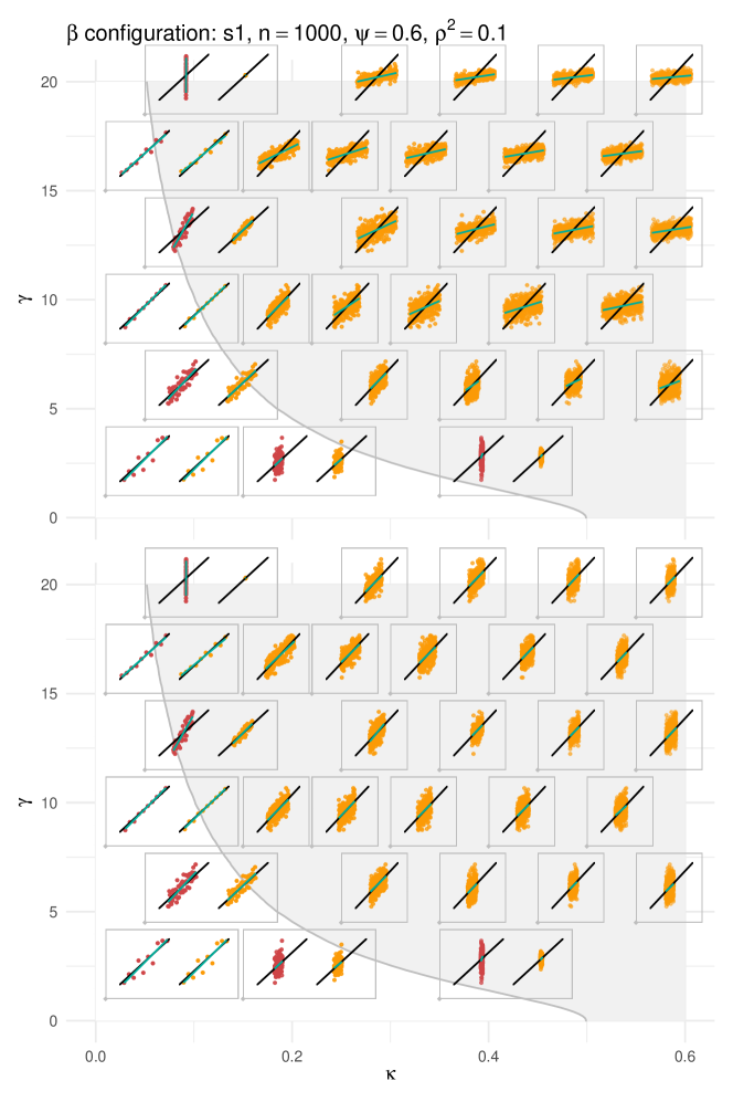
Figure 5: mJPL estimates (top) and their rescaled versions after division by (4) (bottom) for $n=1000$, $\psi=0.6$, $\rho^{2}=0.1$, and $\beta^{*}$ configuration s1 versus $\beta$, with one sample per $(\kappa,\gamma)$ point. The ML estimate exists asymptotically in the white area and does not exist asymptotically in the grey area. The blue lines are from a simple linear regression of the estimates on $\beta$, and the black lines are $45^{o}$ reference lines.

5 Computational performance

Table 2: Summaries on computational performance from using the brglm2 R package for mJPL on data sets from the test phase for $n=2000$ and $\beta^{*}$ configuration s2, on a 2021 MacBook Pro with Apple M1 Max chip and 64 GB RAM. Summaries are over all combinations of $\psi\in\{0,0.3,0.6,0.9\}$ and $\rho^{2}\in\{0,0.1,\ldots,0.9\}$, for each $(\kappa,\gamma)$ point on the panels of Figure 4. $t$ is average computational time in minutes, and $\min k$, $\bar{k}$, and $\max k$ are minimum, average and maximum required number of iterations, respectively). Computational times less than $0.01$ minutes are shown as $0.00$.

$\kappa$	$\gamma$	$p$	$t$	$\min k$	$\bar{k}$	$\max k$
$0.01$	$1.00$	$20$	$0.00$	$3$	$3.00$	$3$
$0.01$	$8.00$	$20$	$0.00$	$7$	$8.82$	$15$
$0.01$	$15.00$	$20$	$0.00$	$9$	$14.00$	$50$
$0.05$	$4.50$	$100$	$0.01$	$6$	$7.53$	$11$
$0.05$	$11.50$	$100$	$0.02$	$11$	$19.00$	$58$
$0.05$	$18.50$	$100$	$0.04$	$16$	$33.58$	$96$
$0.15$	$1.00$	$300$	$0.06$	$3$	$3.10$	$4$
$0.15$	$8.00$	$300$	$0.40$	$10$	$39.50$	$80$
$0.15$	$15.00$	$300$	$0.33$	$8$	$29.55$	$47$
$0.22$	$8.00$	$440$	$0.64$	$7$	$28.32$	$60$
$0.22$	$15.00$	$440$	$0.69$	$5$	$21.85$	$41$
$0.25$	$4.50$	$500$	$1.45$	$11$	$39.02$	$77$
$0.25$	$11.50$	$500$	$0.75$	$5$	$20.43$	$47$
$0.25$	$18.50$	$500$	$0.73$	$5$	$18.10$	$35$
$0.30$	$8.00$	$600$	$1.07$	$5$	$19.20$	$42$
$0.30$	$15.00$	$600$	$0.83$	$4$	$15.03$	$26$
$0.35$	$1.00$	$700$	$0.51$	$5$	$5.95$	$7$
$0.35$	$4.50$	$700$	$1.33$	$7$	$25.15$	$58$
$0.35$	$11.50$	$700$	$0.88$	$6$	$13.95$	$24$
$0.35$	$18.50$	$700$	$0.83$	$6$	$13.78$	$23$
$0.40$	$8.00$	$800$	$1.39$	$8$	$13.55$	$21$
$0.40$	$15.00$	$800$	$1.20$	$8$	$12.35$	$19$
$0.45$	$4.50$	$900$	$1.98$	$9$	$17.62$	$38$
$0.45$	$11.50$	$900$	$1.48$	$8$	$11.57$	$19$
$0.45$	$18.50$	$900$	$1.41$	$7$	$11.30$	$18$
$0.50$	$8.00$	$1000$	$1.71$	$9$	$11.80$	$21$
$0.50$	$15.00$	$1000$	$1.68$	$9$	$11.15$	$17$
$0.55$	$4.50$	$1100$	$1.76$	$11$	$14.00$	$25$
$0.55$	$11.50$	$1100$	$1.74$	$9$	$11.57$	$17$
$0.55$	$18.50$	$1100$	$1.66$	$9$	$11.70$	$15$

Sur and Candès (2019, Supporting Information document, Section D) reports that mJPL has been computationally infeasible for high dimensions, with a runtime of approximately 10 minutes for $n=1000$ and $p=200$, and of over 2.5 hours for $n=2000$ and $p=400$. In notable contrast to the observations in Sur and Candès (2019, Supporting Information document, Section D), for $n=2000$, and configuration s2, the average runtime for mJPL using the brglm2 R package ranges from milliseconds to just below 2 minutes, with no particular care in the choice of starting values. Averages are computed using data sets from the test phase and over all combinations of $\psi\in\{0,0.3,0.6,0.9\}$, $\rho^{2}\in\{0,0.1,\ldots,0.9\}$ for each $(\kappa,\gamma)$ point on the panels of Figure 4. Table 2 provides detailed summaries on computational performance.

Purpose-build implementations for mJPL can result in dramatic reduction in computational times. For example, the repeated ML fits on adjusted responses and totals in Kosmidis and Firth (2021, Section 4), paired with compiled programs for ML estimation of logistic regression models will result in substantially better runtimes.

6 Concluding remarks

6.1 Covariate distribution

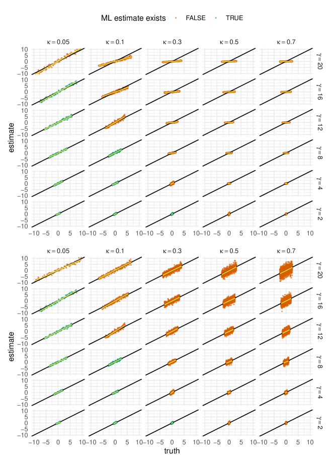
Figure 6: mJPL estimates (top) and their rescaled versions after division by (4) (bottom) for $n=2000$, $\lambda=0.1$, $\rho^{2}=0.3$, and $\beta^{*}$ configuration s1, with one sample per $(\kappa,\gamma)$ combination in the setting of Section 6.1. Existence (green) or not (orange) of the ML estimate is determined using the detectseparation R package for each sample. The yellow lines are from a simple linear regression of the estimates on $\beta$, and the black lines are $45^{o}$ reference lines.

The numerical evidence in Zhao et al. (2022, Section 6) illustrate that their theoretical results for multivariate normal covariates continue to apply for a broad class of covariate distributions with sufficiently light tails. Our empirical experience is that the same holds for Conjecture 1.1! For example, consider a setting where $x_{i}$ consists of independent Bernoulli random variables with probability of success $\lambda=0.1$, and $\beta^{*}$ configuration s2. For each combination of $\kappa\in\{0.05,0.1,0.3,0.5,0.7\}$ and $\gamma\in\{2,4,8,12,16,20\}$, and $\rho^{2}=0.3$, we generate a data set with $n=2000$ as in Section 2.1, with the only difference that $\beta=\gamma_{0}\beta^{*}/(\sqrt{\lambda(1-\lambda)}\lVert L^{\top}\beta^{*}\rVert_{2})$, so that ${\mathop{\rm var}}(x_{i}^{\top}\beta)=\gamma_{0}^{2}$ for independent Bernoulli covariates. In absence of asymptotic theory for the existence of ML when the covariates are realizations of Bernoulli random variables, we determine whether the ML estimate exists for each simulated data set using the detectseparation R package.

Figure 6 shows the mJPL estimates and their rescaled versions after division by the approximation to the aggregate bias parameter in (4) versus $\beta$, where the conditions $\kappa<h_{\rm MLE}(\beta_{0},\gamma_{0})$ and $\kappa>h_{\rm MLE}(\beta_{0},\gamma_{0})$ are replaced by whether the ML estimate exists or not, respectively, at each data set. We should emphasize that our prediction (4) comes from experiments involving model matrices that consist of realizations of independent standard normal random variables. We again observe excellent signal recovery. As in the case of normal covariates, we found that the quality of the approximation $q(\kappa,\gamma,\gamma_{0};b^{*})$ to $\alpha_{\star}$ progressively deteriorates as $\rho^{2}$ increases beyond about $0.7$.

6.2 Estimating constants in Conjecture 1.1

If Conjecture 1.1 holds, even with our predictions $b^{*}$ for $b$, its use in real data applications relies on determining $\kappa$, $\gamma$, $\beta_{0}$, and the existence of the ML estimate. The existence of the ML estimate can be established for any given data set using the linear program in Konis (2007), as is implemented in the detectseparation R package, and $\kappa$ can be estimated as $p/n$. For multivariate normal covariates and potentially other distributions with light tails, the procedure in Zhao et al. (2022, Section 7.1) can be readily used to get estimates for $\beta_{0}$ and $\gamma$. Then an estimate of $\gamma_{0}$ is determined by the relationship $\gamma_{0}=\sqrt{\gamma^{2}-\beta_{0}^{2}}$.

7 Supplementary material

The repository https://github.com/ikosmidis/mJPL-conjecture-supplementary provides code to reproduce the experiments, figures, and tables in the current paper. We also provide R image files with the outputs of all experiments.

8 Declarations

For the purpose of open access, the authors have applied a Creative Commons Attribution (CC BY) licence to any Author Accepted Manuscript version arising from this submission.

References

- Albert and Anderson (1984) Albert, A. and J. Anderson (1984). On the existence of maximum likelihood estimates in logistic regression models. Biometrika 71(1), 1–10.
- Candès and Sur (2020) Candès, E. J. and P. Sur (2020). The phase transition for the existence of the maximum likelihood estimate in high-dimensional logistic regression. Annals of Statistics 48(1), 27–42.
- Firth (1993) Firth, D. (1993). Bias reduction of maximum likelihood estimates. Biometrika 80(1), 27–38.
- Heinze et al. (2023) Heinze, G., M. Ploner, L. Jiricka, and G. Steiner (2023). logistf: Firth’s Bias-Reduced Logistic Regression. R package version 1.25.0.
- Konis (2007) Konis, K. (2007). Linear programming algorithms for detecting separated data in binary logistic regression models. Ph. D. thesis, University of Oxford.
- Kosmidis (2023) Kosmidis, I. (2023). brglm2: Bias Reduction in Generalized Linear Models. R package version 0.9.
- Kosmidis and Firth (2021) Kosmidis, I. and D. Firth (2021). Jeffreys-prior penalty, finiteness and shrinkage in binomial-response generalized linear models. Biometrika 108, 71–82.
- Kosmidis et al. (2020) Kosmidis, I., E. C. Kenne Pagui, and N. Sartori (2020). Mean and median bias reduction in generalized linear models. Statistics and Computing (to appear) 30, 43–59.
- Kosmidis et al. (2022) Kosmidis, I., D. Schumacher, and F. Schwendinger (2022). detectseparation: Detect and Check for Separation and Infinite Maximum Likelihood Estimates. R package version 0.3.
- Mak (2021) Mak, S. (2021). minimaxdesign: Minimax and Minimax Projection Designs. R package version 0.1.5.
- Mak and Joseph (2018) Mak, S. and V. R. Joseph (2018). Minimax and minimax projection designs using clustering. Journal of Computational and Graphical Statistics 27(1), 166–178.
- McCullagh (1987) McCullagh, P. (1987). Tensor Methods in Statistics (1st ed.). Monographs on Statistics and Applied Probability. London ; New York: Chapman and Hall.
- McCullagh and Nelder (1989) McCullagh, P. and J. A. Nelder (1989). Generalized Linear Models (2nd ed.). London: Chapman and Hall.
- Salehi et al. (2019) Salehi, F., E. Abbasi, and B. Hassibi (2019). The Impact of Regularization on High-Dimensional Logistic Regression. Number 1075. Red Hook, NY, USA: Curran Associates Inc.
- Sur and Candès (2019) Sur, P. and E. J. Candès (2019). A modern maximum-likelihood theory for high-dimensional logistic regression. Proceedings of the National Academy of Sciences 116(29), 14516–14525.
- Wedderburn (1974) Wedderburn, R. (1974). Quasi-likelihood functions, generalized linear models, and the Gauss-Newton method. Biometrika 61(3), 439–447.
- Zhao et al. (2022) Zhao, Q., P. Sur, and E. J. Candès (2022). The asymptotic distribution of the MLE in high-dimensional logistic models: Arbitrary covariance. Bernoulli 28(3).