G213.0$-$0.6, a true supernova remnant or just an H ii region?

Abstract

G213.0$-$0.6 is a faint extended source situated in the anti-center region of the Galactic plane. It has been classified as a shell-type supernova remnant (SNR) based on its shell-like morphology, steep radio continuum spectrum, and high ratio of [S ii]/H$\alpha$. With new optical emission line data of H$\alpha$, [S ii], and [N ii] recently observed by the Large Sky Area Multi-Object Fiber Spectroscopic Telescope, the ratios of [S ii]/H$\alpha$ and [N ii]/H$\alpha$ are re-assessed. The lower values than those previously reported put G213.0$-$0.6 around the borderline of SNR-H ii region classification. We decompose the steep-spectrum synchrotron and the flat-spectrum thermal free-free emission in the area of G213.0$-$0.6 with multi-frequency radio continuum data. G213.0$-$0.6 is found to show a flat spectrum, in conflict with the properties of a shell-type SNR. Such a result is further confirmed by TT-plots made between the 863-MHz, 1.4-GHz, and 4.8-GHz data. Combining the evidence extracted in both optical and radio continuum, we argue that G213.0$-$0.6 is possibly not an SNR, but an H ii region instead. The $V_{LSR}$ pertaining to the H$\alpha$ filaments places G213.0$-$0.6 approximately 1.9 kpc away in the Perseus Arm.

1 Introduction

G213.0$-$0.6 is a faint extended source located in the anti-center region of the Galactic plane. It has been proposed to be a shell-type supernova remnant (SNR) by Reich et al. (2003) based on its morphology and the radio continuum spectral index of $\alpha=-0.40\pm 0.15$ ($S_{\nu}\sim\nu^{\alpha}$, with $S_{\nu}$ being the flux density at frequency $\nu$), derived from a 30^′-wide region across the source between the Effelsberg 863-MHz and 2695-MHz data. An even earlier study partially relevant to this target was conducted by Bonsignori-Facondi & Tomasi (1979). They proposed the existence of another SNR G211.7$-$1.1, which coincides with the nearby H ii region SH 2-284 (Sharpless, 1959) and includes the strong shell-like structure of G213.0$-$0.6 (see Fig. 11 in their work). Stupar & Parker (2012) studied G213.0$-$0.6 using optical observations. They confirmed it to be an SNR based on the high [S ii]/H$\alpha$ ratio of 0.5 $-$ 1.1 for some of its bright filaments. They also adjusted the name to G213.3$-$0.4 according to a newly determined geometric center. In this work, we adhere to the name of “G213.0$-$0.6” in line with SNR catalogs (e.g. Green, 2019) and other references.

Based on the spatial correlation with CO clouds, the distance of G213.0$-$0.6 was suggested to be approximately 1 kpc (Su et al., 2017). This is supported by the distance assessments from optical and dust extinction analysis (Yu et al., 2019; Zhao et al., 2020). The apparent size $160\hbox{${}^{\prime}$}\times 140\hbox{${}^{\prime}$}$ of G213.0$-$0.6 therefore corresponds to the physical extent of 46 pc $\times$ 40 pc. The prominent H ii region SH 2-284, close to G213.0$-$0.6 in the sky, has a distance of about 4 kpc (Cusano et al., 2011) or 4.5 kpc (Negueruela et al., 2015). This implies no physical connection between G213.0$-$0.6 and SH 2-284.

Until now, studies that are focused on G213.0$-$0.6 are still very limited, possibly because it is too faint and extended to be well observed. In this paper, we aim to re-investigate the nature of G213.0$-$0.6 by combining the recently observed optical spectral line data from the Large Sky Area Multi-Object Fiber Spectroscopic Telescope (LAMOST) and sensitive multi-frequency radio continuum data which are public. In the following, we first introduce the LAMOST optical emission line data and present the line ratios of [S ii]/H$\alpha$ and [N ii]/H$\alpha$ newly derived from the data in Sect. 2. We show radio continuum images derived from the component separation and the spectrum determined through TT-plots in Sect. 3. The morphology, distance, and the possible ionizing source related to G213.0$-$0.6 are discussed in Sect. 4. The intriguing characteristics of G213.0$-$0.6 are summarized in Sect. 5.

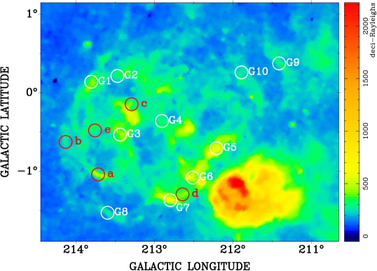
Figure 1: H$\alpha$ emission in the area of G213.0$-$0.6 extracted from the Southern H$\alpha$ Sky Survey Atlas (Gaustad et al., 2001). Five positions (red open circles labeled with “a” to “e”) from Stupar & Parker (2012) and ten extra positions (white open circles starting with “G”) selected in this work are used to derive the properties of the optical emission lines as listed in Table 1.

2 Optical emission lines

H$\alpha$ images of G213.0$-$0.6 were shown in Stupar & Parker (2012) with both the high-resolution data from the Anglo-Australian Observatory/United Kingdom Schmidt Telescope (AAO/UKST) H$\alpha$ survey of the southern Galactic plane (Parker et al., 2005) and the lower-resolution but high-sensitivity data from the Southern H$\alpha$ Sky Survey Atlas (hereafter SHASSA, Gaustad et al., 2001). Their follow-up optical spectral observations, which were used for the estimates of spectral line ratios, were made with the 1.9-m Radcliffe telescope of the South African Astronomical Observatory. In this work, we present the H$\alpha$ image of G213.0$-$0.6 using SHASSA data in Fig. 1, because they better show the complete shell structure of G213.0$-$0.6 as pointed out by Stupar & Parker (2012). The spectral data used for analysis are from LAMOST, a powerful instrument for optical spectroscopy (Cui et al., 2012), which is a four-meter reflecting Schmidt telescope outfitted with 4 000 fibers distributed on its focal plane. We extract the processed data products from the project of the LAMOST Medium-Resolution Spectral survey (MRS, Liu et al., 2020) of Galactic Nebulae (MRS-N, Wu et al., 2021). They were observed in November 2021. The wavelength range covered by the MRS-N comprises two segments: the red arm spanning 6300Å to 6800Å  and the blue arm encompassing 4950Å to 5350Å. Within the red arm, notable nebular emission lines, i.e. H$\alpha$, [N ii]$\uplambda\uplambda$6548,6584 and [S ii]$\uplambda\uplambda$6717,6731, have been recorded with a relatively high spectral resolution (R$\sim$7500). Ren et al. (2021) introduced a method to re-calibrate wavelengths and achieve a radial velocity measurement precision better than 1 km/s. Zhang et al. (2021) outlined a technique to subtract geo-coronal H$\alpha$ emission, that successfully reduced the contamination level of the geo-coronal H$\alpha$ line from 40% to below 10%. The detailed data processing procedure can be referred to Wu et al. (2022).

Stupar & Parker (2012) analyzed spectral line ratios at five positions on some of the prominent filaments of G213.0$-$0.6 and showed that all the five [S ii]/H$\alpha$ ratios exceed 0.5, with a maximum of 1.1, favoring a shock-excited SNR origin. With the new LAMOST data, we take measurements not only for the five positions (denoted as "a" to "e" in Fig. 1) selected in Stupar & Parker (2012), but also add ten additional positions on other bright filaments, labeled from “G1” to “G10” in Fig. 1. Because the separation of two adjacent fibers of LAMOST is about 2^′, the best spectra data within a radius of 5 ^′ of each position with a signal-to-noise ratio over 10 are chosen to make the average. The results are compiled in Table 1.

Table 1: Properties of the optical spectral lines in the area of G213.0$-$0.6 observed by the LAMOST MRS-N. The 1st $-$ 3rd columns present the reference name and their coordinates marked in Fig. 1. The 4th column shows the $V_{LSR}$ measured for the H$\alpha$ line. The spectral line ratio of [N ii]/H$\alpha$ and [S ii]/H$\alpha$ measured in this work are listed in the 5th and 7th column. The values reported in Stupar & Parker (2012), abbreviated as “S12” are presented in the 6th and 8th column for comparison. The ratio between the doublets of [S ii] and the estimates of the electron density are shown in the 9th and 10th column.

Reference	RA (J2000)	Dec (J2000)	$V_{LSR}$	[N ii]/H$\alpha$	[N ii]/H$\alpha$	[S ii]/H$\alpha$	[S ii]/H$\alpha$	[S ii]	Electron density
	(h m s)	(d m s)	(km/s)	this work	S12	this work	S12	(6717/6731Å)	(cm-3)
(1)	(2)	(3)	(4)	(5)	(6)	(7)	(8)	(9)	(10)
a	06 49 09	$-$01 10 30	15.6	0.45	0.76	0.44	0.6	1.27	140
b	06 51 22	$-$01 21 17	13.6	0.40	0.59	0.36	0.8	1.49	20
c	06 51 33	$-$00 23 03	22.7	0.42	0.50	0.41	0.5	1.59	10
d	06 46 16	$-$00 20 07	22.6	0.39	0.58	0.51	1.1	1.45	30
e	06 51 13	$-$00 57 03	12.8	0.45	0.88	0.38	1.0	1.50	19
G1	06 53 30	$-$00 42 58	18.1	0.42	$-$	0.45	$-$	1.41	50
G2	06 53 09	$-$00 23 11	12.5	0.47	$-$	0.48	$-$	1.50	19
G3	06 50 26	$-$00 41 51	25.1	0.49	$-$	0.38	$-$	1.42	44
G4	06 50 05	$-$00 08 30	17.7	0.32	$-$	0.32	$-$	1.29	120
G5	06 47 36	$+$00 18 56	27.1	0.37	$-$	0.37	$-$	1.43	30
G6	06 46 48	$-$00 07 22	30.6	0.35	$-$	0.41	$-$	1.46	30
G7	06 46 18	$-$00 30 24	22.4	0.36	$-$	0.42	$-$	1.37	70
G8	06 47 11	$-$01 17 29	6.1	0.29	$-$	0.43	$-$	1.35	90
G9	06 49 58	$+$01 31 12	26.8	0.43	$-$	0.55	$-$	1.51	10
G10	06 50 26	$+$01 02 35	24.7	0.53	$-$	0.59	$-$	1.30	110

The LAMOST measurements (see Table 1) show that the [S ii]/H$\alpha$ and [N ii]/H$\alpha$ ratios for the five common positions as in Stupar & Parker (2012) are mostly below 0.5. Some are nearly half of the values previously reported. For the rest ten positions newly selected in this work, the results are consistent with the new values for the five common positions. The average values of [S ii]/H$\alpha$ and [N ii]/H$\alpha$ for all the 15 positions are about 0.43 and 0.41, respectively. The criterion value of [S ii]/H$\alpha$ ratio to distinguish SNRs and H ii regions has long been discussed. Besides the value of 0.5 as quoted in e.g. Stupar & Parker (2012), 0.4 and 2/3 were also adopted (see Fesen et al., 1985, and references therein). To solve the ambiguity when 0.4 < [S ii]/H$\alpha$ < 2/3, Fesen et al. (1985) suggested to use the line ratios of [O i]/H$\beta$ and [O ii]/H$\beta$ to aid the classification. In a recent work, Kopsacheili et al. (2020) explored more efficient 3D and 2D diagnostic tools by using [O i]/H$\alpha$ $-$ [O ii]/H$\beta$ $-$ [O iii]/H$\beta$ and [O i]/H$\alpha$ $-$ [O iii]/H$\beta$ with a low confusion in classification. However, our LAMOST data do not cover [O ii]($\mathrm{\uplambda\uplambda 3727,3729}$) or H$\beta$($\uplambda 4862$). The [O i]($\uplambda$ 6300) line is contaminated by the skylight. In particular, we notice that even if the criterion value of [S ii]/H$\alpha$ is set to 0.4, one still cannot completely rule out some H ii regions that could be mistaken as SNRs (see Kopsacheili et al., 2020, in their Fig. 5). Different values of [S ii]/H$\alpha$ both greater and less than 0.4 are also seen within the same H ii region (e.g., Li et al., 2022). Another method utilizing optical emission line ratios, considering both log([S ii]/H$\alpha$) and log([N ii]/H$\alpha$), has been employed by e.g. Kniazev et al. (2008); Lagrois et al. (2012) and Sabin et al. (2013). The average values from the LAMOST measurements correspond to log([S ii]/H$\alpha$) $\sim$ $-$0.36 and log([N ii]/H$\alpha$) $\sim$ $-$0.39, also placing G213.0$-$0.6 in the borderline area between “H ii region” and “SNR” (see Fig. 4 in Kniazev et al., 2008). Thus, the current LAMOST data are not sufficient to make a definite classification, but could raise a question about the identity of G213.0$-$0.6 as being an SNR.

3 Thermal emission nature revealed by Radio continuum

Radio continuum emission and the corresponding spectral index provide another useful tool in distinguishing between SNRs and H ii regions (e.g. Foster et al., 2006; Gao et al., 2011). Shell-type SNRs have steep-spectrum synchrotron emission (e.g. Dubner & Giacani, 2015), while the optical-thin free-free emission from H ii regions shows a flat spectrum ($\alpha\sim-0.1$, $S_{\nu}\sim\nu^{\alpha}$). With publicly available radio continuum data, we investigate the radio continuum emission properties of G213.0$-$0.6 via two methods in the following.

3.1 Component separation

By using multi-frequency radio continuum data, Paladini et al. (2005) developed a method to decompose the mixed signal from the Galaxy into non-thermal synchrotron emission stemming from relativistic electrons spiraling in the magnetic field and thermal free-free emission from ionized gas. Based on this method, Sun et al. (2011) separated the two emission components in the inner Galactic plane area with $10\hbox{${}^{\circ}$}\leq\ell\leq 60\hbox{${}^{\circ}$}$, and $|b|\leqslant 4\hbox{${}^{\circ}$}$, while Xu et al. (2013) scoured the Cygnus-X complex for new SNRs by singling out synchrotron emission from strong confusing thermal emission. These successful applications make the method useful in fast recognition of the emission nature of radio sources in vast sky areas.

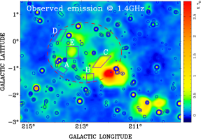
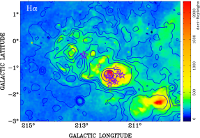
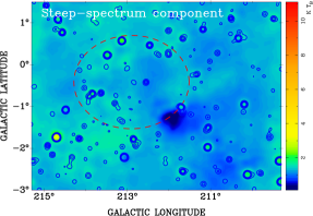
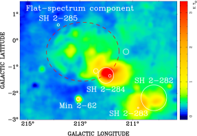
Figure 2: Upper-left panel: Effelsberg 1.4-GHz total-intensity (source component) image for the area of G213.0$-$0.6 at a resolution of 9$.\mkern-4.0mu^{\prime}$4. The large-scale diffuse Galactic background emission is not included. The ellipse enclosed by the red dashed line outlines G213.0$-$0.6. The blue contours indicate strong point-like sources in the NVSS (Condon et al., 1998) smoothed to 6^′. The polygon areas illustrated by the purple lines and marked as “A” to “E” are used for TT-plots to derive the spectra of G213.0$-$0.6. Lower-left and lower-right panels: images of the separated steep-spectrum and the flat-spectrum components smoothed to a resolution of 11^′, including the Galactic large-scale emission. The WISE H ii regions (Anderson et al., 2014) are illustrated by white circles in the lower-right panel with sizes representing their angular extent. The circles with names aside are H ii regions which have also been identified in previous optical observations (Sharpless, 1959; Frew et al., 2013). In the upper-right panel, H$\alpha$ emission extracted from SHASSA (Gaustad et al., 2001) is presented overlaid by contours of the separated flat-spectrum radio emission. The purple stars are OB-type stars observed by Gaia and extracted from Xu et al. (2021). The sizes of the stars are scaled according to their distance as listed in Table 2.

We improve the work of Xu et al. (2013) by considering the steepening of the synchrotron spectrum at higher frequencies and apply the algorithm to the anti-center region of the Galactic plane. The result indicates a strong tendency that G213.0$-$0.6 is a thermal-emitting source rather than an SNR. We briefly explain the procedure and show the results in below.

Paladini et al. (2005) derived the thermal emission fraction via:

$$f_{\rm th,\nu_{1}}=\frac{T_{\rm ff,\nu_{1}}}{T_{\rm gal,\nu_{1}}}=\frac{T_{\rm ff,\nu_{1}}}{T_{\rm ff,\nu_{1}}+T_{\rm syn,\nu_{1}}}=\frac{1-(\nu_{2}/\nu_{1})^{\rm\beta_{gal}-\beta_{syn}}}{\rm 1-(\nu_{2}/\nu_{1})^{\beta_{ff}-\beta_{syn}}}$$ (1)

Here, $f_{\rm th,\nu_{1}}$ is the fraction of the thermal component at frequency $\nu_{1}$, $T_{\rm gal}$ refers to the total Galactic emission, i.e. the sum of non-thermal emission $T_{\rm syn}$ and the thermal emission $T_{\rm ff}$. The parameters $\beta_{\rm gal}$, $\beta_{\rm syn}$, and $\beta_{\rm ff}$ are the brightness-temperature spectral indices of the Galactic, synchrotron and free-free emission, respectively (T${}_{\nu}\sim\nu^{\beta}$, $\beta=\alpha-2$). The value of $\beta_{\rm gal}$ can be conveniently calculated from the observational data at a second frequency $\nu_{2}$ through $\beta_{\rm gal}={\rm log}(T_{\rm gal,\nu_{1}}/T_{\rm gal,\nu_{2}})/{\rm log}({\rm\nu_{1}}/{\rm\nu_{2}})$, and $\beta_{\rm ff}$ is usually set to a fixed value of $-$2.1 (e.g. Paladini et al., 2005) or alternatively $-$2.15 (e.g. Bennett et al., 2013). Here, we adopt $\beta_{\rm ff}=-2.15$. $\beta_{\rm syn}$ is the only unknown in the expression.

We use four data sets for component separation. These are the 408-MHz all-sky survey data (Haslam et al., 1982), which were de-striped by Remazeilles et al. (2015), the Effelsberg 1408-MHz survey data (Reich et al., 1997), the 9-yr WMAP K-band (22.8-GHz) data (Bennett et al., 2013), and the Urumqi 4.8-GHz survey data of Gao et al. (2010). As in Xu et al. (2013), after corrected for the offset values such as errors in zero levels, the cosmic microwave background, and the unresolved extra-galactic sources, the data of 408 MHz v.s. 1408 MHz and the data of 1408 MHz v.s. 22.8 GHz at a common angular resolution of 1^∘ are split into two groups. Because the thermal emission at 1.4 GHz calculated from the first data pair should be the same as that obtained from the second data pair, one can find the best-fit value of $\beta_{\rm syn}$ for each pixel to balance the two sides and then obtain the total amount of flat-spectrum and steep-spectrum emission components at 1.4 GHz. Meanwhile, one can also get the Galactic emission template at any frequency $\nu$ following $T_{\rm gal,\nu}=T_{\rm syn,1.4~{}GHz}\cdot(\nu/1.4)^{\beta_{\rm syn}}+T_{\rm ff,1.4~{}GHz}\cdot(\nu/1.4)^{\beta_{\rm ff}}$. This template is used to compensate the missing large-scale structure in the Urumqi 4.8-GHz total-intensity data. Subsequently, by using the 9$.\mkern-4.0mu^{\prime}$5 resolution data at 4.8 GHz and 1.4 GHz, together with the synchrotron spectral indices found above, we could decompose the Galactic emission via Eq. 1.

In practice, the synchrotron spectrum is not a perfect single-power law but steepens as the observing frequency increases. Jaffe et al. (2011) found $-2.8<\beta_{\rm syn}<-2.74$ from 408 MHz to 2.3 GHz and $-2.98<\beta_{\rm syn}<-2.91$ from 2.3 GHz to 23 GHz. The model proposed by Kogut (2012) showed consistent values, also with a difference of $\Delta\beta_{\rm syn}\sim 0.2$ between the low- and high-frequency data pairs. Based on this information, we treat the synchrotron spectral index $\beta_{\rm syn}$ as two separate variables for the two groups rather than maintaining the same value as in Xu et al. (2013). We seek for the best fit on the two sides by constraining the difference of $\beta_{\rm syn}$ between the two data pairs.

The decomposition results made for the 1.4-GHz data after considering the synchrotron spectrum steepening are shown in Fig. 2. The uncertainty, including those in the input data sets and by the error propagation, is typically $\sim$15%, lower than those in Xu et al. (2013). At a first glance, many compact radio sources are seen overlaid on the non-thermal background, however, almost all the prominent extended radio sources are presented in the flat-spectrum component image. They are mostly known H ii regions, i.e. SH 2-282 to 285 and Min 2-62 (white circles in the lower-right panel of Fig. 2). Notably, G213.0$-$0.6 also appears to have a flat spectrum, not only the filaments that can be resolved in the northeast, southeast, south, but also the strong and thick shell structure in its southwest, where the thermal emission fraction can reach $\sim$60%. These separated radio continuum flat-spectrum structures correlate well with the H$\alpha$ emission (Gaustad et al., 2001) of G213.0$-$0.6 as shown in the upper-right panel of the Fig. 2.

Figure 3: TT-plots made for the spectral indices by using the data between 1.4 GHz (Effelsberg) and 4.8 GHz (Urumqi) at a common angular resolution of 9$.\mkern-4.0mu^{\prime}$5 (left panels) and the data between 863 MHz (Effelsberg) and 4.8 GHz (Urumqi) at an angular resolution of 14$.\mkern-4.0mu^{\prime}$5 (right panels) in the regions “A” to “E” as marked in the upper-left panel of Fig. 2. To avoid confusion from ambient point-like sources, the sizes of region A and D are slightly reduced for the 863-MHz and the 4.8-GHz images at 14$.\mkern-4.0mu^{\prime}$5 resolution.

3.2 Radio continuum spectrum

The component-separation results can be regarded as a hint for the emission nature of radio sources. The method is convenient for a quick view of numerous radio structures in a vast sky area. However, we note that the r.m.s noise level, i.e. 30 $-$ 50 mK $T_{b}$ of the background emission in the separation results is higher than that in the input survey map, i.e. $\sim$16 mK $T_{b}$ for the Effelsberg 1.4-GHz survey data. The decomposition method hence can work well on structures with strong emission, but has some limitations for the structural features that are too faint.

To confirm the overall spectrum nature of G213.0$-$0.6, we make TT-plots (Turtle et al., 1962) between the observed Effelsberg 1.4-GHz and the Urumqi 4.8-GHz data, and between the archived Effelsberg 863-MHz (Reich et al., 2003) and the Urumqi 4.8-GHz data. The inclusion of the Urumqi 4.8-GHz data, which was not available at the time of Reich et al. (2003), significantly widens the frequency range than before (863-MHz v.s. 2.7-GHz) and will lead to smaller uncertainties in determining spectral indices. Furthermore, the NVSS sources are first overlaid onto the image, and five areas free from strong point-like sources are selected (as marked with “A” to “E” in the upper-left panel of Fig. 2) for this purpose. We show the TT-plot results for the five regions in Fig. 3. The spectral indices of $\beta\sim-1.84$ to $-$2.17 ($\alpha=\beta+2$) confirm and strongly support the flat-spectrum thermal emission nature of G213.0$-$0.6. TT-plots toward the 30^′ wide stripe centered at $b=-10\hbox{${}^{\prime}$}$ as indicated in Reich et al. (2003) is also tested, but show scattered data points. We believe this is affected by the existence of un-resolved point-like sources in the upper part of G213.0$-$0.6 (see upper-left panel in Fig. 2). They are very difficult to be removed in view of the 14$.\mkern-4.0mu^{\prime}$5 resolution of the 863-MHz data.

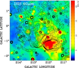
Figure 4: IRIS 60$\mu$m infrared emission of the G213.0$-$0.6 area. The contours are from the Effelsberg 2.7-GHz radio continuum data smoothed to a resolution of 6^′ to increase the signal-to-noise ratio.

4 Discussion

4.1 Morphology

The morphology of G213.0$-$0.6 has been discussed in detail by Stupar & Parker (2012). The filamentary structures seen in both optical H$\alpha$ and at radio frequencies are well correlated. However, H ii regions and SNRs could share such a feature, e.g. the H ii region Carina Nebula (Smith et al., 2010; Rebolledo et al., 2021) and the SNR S147 (Greimel et al., 2021; Xiao et al., 2008). The H$\alpha$ emission of H ii regions comes from recombination of electrons and protons, and the radio emission is from the free-free emission in the same ionized gas. The H$\alpha$ and radio emission of SNRs originates from the shock-excited interstellar medium and synchrotron emission from shock-accelerated relativistic electrons, respectively. Therefore, a solid classification cannot be made by morphological features, but needs proofs, e.g. in optical emission-line ratios and radio continuum spectrum. Stupar & Parker (2012) examined the infrared emission which traces dust in the area of G213.0$-$0.6. They presented a color-coded (RGB, red for radio continuum, green for 60$\mu$m infrared, and blue for H$\alpha$) image and stated that there is no clear morphological association between the infrared and the well-correlated optical-radio emission. We present the IRIS 60$\mu$m image (Miville-Deschênes & Lagache, 2005) in Fig. 4 and overlay the radio continuum contours of the Effelsberg 2.7-GHz data (Fürst et al., 1990). Unlike the infrared emission filling the entire H ii region SH 2-284, the 60$\mu$m emission in the area of G213.0$-$0.6 is relatively weaker. However, it is difficult to conclude that there is no morphological association, because some infrared emission seems to be confined along the radio boundary. It is also not clear that in case the dust was cleared away by the stellar winds as G213.0$-$0.6 evolves, resulting in low infrared emission in the field.

The X-ray source 1RXS J065049.7$-$003220 was proposed to be possibly associated with G213.0$-$0.6 (Stupar & Parker, 2012). Based on machine learning, McGlynn et al. (2004) developed the tool of “ClassX” to classify ROSAT sources (Voges et al., 1999). The X-ray emission from 1RXS J065049.7$-$003220 most probably stems from a star. Haakonsen & Rutledge (2009) cross-matched the sources in the ROSAT All Sky Survey Bright Source Catalog and the near-infrared sources from the Two Micron All Sky Survey Point Source Catalog (Cutri et al., 2003). They found that 1RXS J065049.7$-$00322 may be associated with a star in binary system. Hence, the X-ray emission seen inside G213.0$-$0.6 seems not related.

4.2 Distance and possible ionizing source

The radial velocity (V_LSR) measured for the H$\alpha$ line in the selected positions exhibits positive values averaged to around 20 km/s, except for the position G8 with approximately 6 km/s. The origin of this singular V_LSR value is ambiguous; it could reflect the inherent filament motion in this segment of G213.0$-$0.6 or just simply an overlap in a nearer distance, considering that it is located far away from the major part of G213.6$-$0.6. According to Reid et al. (2014), V_LSR $\sim$ 20 km/s approximates the kinematic distance of 1.9${}^{+0.8}_{-0.7}$ kpc, placing G213.0$-$0.6 in the Perseus Arm (Hou, 2021), although with large uncertainties. The physical size of G213.0$-$0.6 is therefore about 87 pc $\times$ 76 pc.

With the Gaia Early Data Release 3 (EDR3, Gaia Collaboration, 2022), Xu et al. (2021) used OB stars with parallax angles to outline the local spiral structures within approximately 5 kpc from the Sun. We extract OB stars in the field of G213.0$-$0.6 and the adjacent H ii region SH 2-284 from Xu et al. (2021). About 30 stars are pinpointed, and their distances are estimated using the parallax angles. There are several OB-type stars in the area with distances ranging from 0.7 $-$ 5 kpc (see Table 2). Among them, two B-type stars, Gaia DR3 3113244500922158464 and Gaia DR3 3113430696344419072 are located in close proximity to the center of G213.0$-$0.6 (see the upper-right panel of Fig. 2 and Table 2). Distinct distances can be directly estimated from the parallax angle for the two stars: one at $\sim$0.7 kpc and the other at $\sim$4.2 kpc. Neither of the two stars seems to be related in view of distances. However, the distance of the latter, Gaia DR3 3113430696344419072 reduces to $\sim$2.7 kpc after the correction by Gaia Collaboration (2022), which largely narrows the gap and makes it comparable to the kinematic distance inferred from the V_LSR of the H$\alpha$ filaments.

Within the core and outer regions of the H ii region SH 2-284, a cluster of stars is found. The majority of these stars are positioned at distances ranging from approximately 4 to 5 kpc. Some of them are responsible for the ionization of SH 2-284 (e.g Negueruela et al., 2015). A B1II-type star is situated at the center of the shell region between G213.0$-$0.6 and SH 2-284. The distance for this star estimated from the parallax-angle measurement is consistent with those in SH 2-284. Therefore, it might be possible that the radio emission from the shell region originates from the contribution of G213.0$-$0.6 itself and partially from the ionized gas created by this star, assuming that it is indeed capable to generate an H ii region from the same line of sight.

5 Summary

The low surface-brightness extended radio source G213.0$-$0.6 was previously suggested to be an SNR. We revisit the nature of G213.0$-$0.6 by combining the optical spectral line data together with the radio continuum data. The new LAMOST observations of H$\alpha$, [S ii], and [N ii] show lower spectral line ratios in comparison to previous results, shaking the identify of G213.0$-$0.6 as being an SNR. Multi-wavelength radio continuum images are used to separate non-thermal synchrotron emission from the thermal free-free emission. Both the decomposition result and the additional verification made by TT-plots confirm that G213.0$-$0.6 has a flat spectrum, the key feature of thermal emission. OB-type stars are the ionizing sources of H ii regions. The B-type star located at $\ell=212\hbox{$.\!\!^{\circ}$}93$, $b=-0\hbox{$.\!\!^{\circ}$}48$ might be responsible for the ionization of G213.0$-$0.6 due to the comparable distances inferred from the parallax angle (2.7 kpc) and from the $V_{LSR}$ measured for the H$\alpha$ lines (1.9${}^{+0.8}_{-0.7}$ kpc).

Combining all these evidence, we argue that G213.0$-$0.6 is possibly not an SNR at a distance of 1 kpc, but an H ii region located in the Perseus Arm. A further exploration of the optical lines of [O i], [O ii], [O iii], and H$\beta$ would help to reach a solid confirmation about the genuine nature of G213.0$-$0.6.

Data Availability

The data underlying this article will be shared on reasonable request to the corresponding author.

Appendix A Auxiliary Table

Table 2: OB stars around the center of G213.0$-$0.6, the southwest shell and the H ii region SH 2-284. The sequential number and the names of the stars are listed in the 1st and 2nd column. The Galactic coordinates are shown in the 3rd and 4th column. The parallax angle from Gaia Collaboration (2022), the distance derived directly from the parallax angle (d = 1 A.U. / tan(parallax angle)), and the distance after correction by Gaia Collaboration (2022) are presented in 5th $-$ 7th column. The spectral type of the stars extracted from Xu et al. (2021) are given in the 8th column.

No.	Name	Galactic longitude	Galactic latitude	Plx	Distance	Distance∗	SpecType
		(∘)	(∘)	(mas)	(pc)	(pc)
	G213.0$-$0.6
1	Gaia DR3 3113244500922158464	212.93	$-$0.48	0.2362	4235	2768	B0:
2	Gaia DR3 3113430696344419072	212.90	$-$0.53	1.4960	669	$\cdots$	B2V
	Southwest shell region
3	Gaia DR3 3113482545188572928	212.33	$-$0.91	0.2221	4504	3894	B1II
	SH 2-284 and surroundings
4	Gaia DR3 3125505326881596544	212.04	$-$1.28	0.2355	4248	3416	B2V
5	Gaia DR3 3125505563098855552	212.01	$-$1.32	0.2131	4694	3942	B2III
6	Gaia DR3 3125505670478616192	212.00	$-$1.31	0.2281	4386	3303	O7Vz
7	Gaia DR3 3125513878155537024	211.96	$-$1.15	0.1818	5503	$\cdots$	B0Ve
8	Gaia DR3 3119511442321221120	211.95	$-$1.63	0.1914	5227	2819	B2IV
9	Gaia DR3 3119511854638059136	211.94	$-$1.60	0.2389	4187	4536	B2IV
10	Gaia DR3 3125518039984467328	211.93	$-$1.39	0.2479	4035	2943	O9.7V + B
11	Gaia DR3 3125525629188072704	211.86	$-$1.31	0.2010	4977	3360	B2IV
12	Gaia DR3 3125522742970050304	211.81	$-$1.43	0.1579	6336	4336	B1Ve
13	Gaia DR3 3125522197512839680	211.77	$-$1.50	0.2663	3757	3637	B1.5V
14	Gaia DR3 3125522197512841856	211.77	$-$1.51	0.2253	4440	5223	B1.5V
15	Gaia DR3 3125557828561213568	211.72	$-$1.00	0.2237	4472	3640	B2III
16	Gaia DR3 3125569545232312320	211.70	$-$1.53	0.2220	4506	3309	B2IV
17	Gaia DR3 3125603973689913856	211.63	$-$1.17	0.2201	4545	4888	O8.5Ib(f)
18	Gaia DR3 3125580780866556416	211.63	$-$1.25	0.5957	1679	1357	B0.5IV
19	Gaia DR3 3125585969186497280	211.48	$-$1.26	0.2400	4168	3756	B1.5II-III
20	Gaia DR3 3125597681559414784	211.46	$-$1.28	0.2481	4032	2807	O8Vz + B0:V:

References

- Anderson et al. (2014) Anderson L. D., Bania T. M., Balser D. S., Cunningham V., Wenger T. V., Johnstone B. M., Armentrout W. P., 2014, ApJS, 212, 1
- Bennett et al. (2013) Bennett C. L., et al., 2013, ApJS, 208, 20
- Bonsignori-Facondi & Tomasi (1979) Bonsignori-Facondi S. R., Tomasi P., 1979, A&A, 77, 93
- Condon et al. (1998) Condon J. J., Cotton W. D., Greisen E. W., Yin Q. F., Perley R. A., Taylor G. B., Broderick J. J., 1998, AJ, 115, 1693
- Cui et al. (2012) Cui X.-Q., et al., 2012, Research in Astronomy and Astrophysics, 12, 1197
- Cusano et al. (2011) Cusano F., et al., 2011, MNRAS, 410, 227
- Cutri et al. (2003) Cutri R. M., et al., 2003, 2MASS All Sky Catalog of point sources.
- Dubner & Giacani (2015) Dubner G., Giacani E., 2015, A&ARv, 23, 3
- Fesen et al. (1985) Fesen R. A., Blair W. P., Kirshner R. P., 1985, ApJ, 292, 29
- Foster et al. (2006) Foster T., Kothes R., Sun X. H., Reich W., Han J. L., 2006, A&A, 454, 517
- Frew et al. (2013) Frew D. J., Bojičić I. S., Parker Q. A., 2013, MNRAS, 431, 2
- Fürst et al. (1990) Fürst E., Reich W., Reich P., Reif K., 1990, A&AS, 85, 691
- Gaia Collaboration (2022) Gaia Collaboration 2022, VizieR Online Data Catalog, p. I/355
- Gao et al. (2010) Gao X. Y., et al., 2010, A&A, 515, A64
- Gao et al. (2011) Gao X. Y., Han J. L., Reich W., Reich P., Sun X. H., Xiao L., 2011, A&A, 529, A159
- Gaustad et al. (2001) Gaustad J. E., McCullough P. R., Rosing W., Van Buren D., 2001, PASP, 113, 1326
- Green (2019) Green D. A., 2019, Journal of Astrophysics and Astronomy, 40, 36
- Greimel et al. (2021) Greimel R., et al., 2021, A&A, 655, A49
- Haakonsen & Rutledge (2009) Haakonsen C. B., Rutledge R. E., 2009, ApJS, 184, 138
- Haslam et al. (1982) Haslam C. G. T., Salter C. J., Stoffel H., Wilson W. E., 1982, A&AS, 47, 1
- Hou (2021) Hou L. G., 2021, Frontiers in Astronomy and Space Sciences, 8, 103
- Jaffe et al. (2011) Jaffe T. R., Banday A. J., Leahy J. P., Leach S., Strong A. W., 2011, MNRAS, 416, 1152
- Kniazev et al. (2008) Kniazev A. Y., Pustilnik S. A., Zucker D. B., 2008, MNRAS, 384, 1045
- Kogut (2012) Kogut A., 2012, ApJ, 753, 110
- Kopsacheili et al. (2020) Kopsacheili M., Zezas A., Leonidaki I., 2020, MNRAS, 491, 889
- Lagrois et al. (2012) Lagrois D., Joncas G., Drissen L., 2012, MNRAS, 420, 2280
- Li et al. (2022) Li Y., et al., 2022, Research in Astronomy and Astrophysics, 22, 075010
- Liu et al. (2020) Liu C., et al., 2020, arXiv e-prints, p. arXiv:2005.07210
- McGlynn et al. (2004) McGlynn T. A., et al., 2004, ApJ, 616, 1284
- Miville-Deschênes & Lagache (2005) Miville-Deschênes M.-A., Lagache G., 2005, ApJS, 157, 302
- Negueruela et al. (2015) Negueruela I., Simón-Díaz S., Lorenzo J., Castro N., Herrero A., 2015, A&A, 584, A77
- Paladini et al. (2005) Paladini R., De Zotti G., Davies R. D., Giard M., 2005, MNRAS, 360, 1545
- Parker et al. (2005) Parker Q. A., et al., 2005, MNRAS, 362, 689
- Rebolledo et al. (2021) Rebolledo D., Green A. J., Burton M. G., Breen S. L., Garay G., 2021, ApJ, 909, 93
- Reich et al. (1997) Reich P., Reich W., Fürst E., 1997, A&AS, 126, 413
- Reich et al. (2003) Reich W., Zhang X., Fürst E., 2003, A&A, 408, 961
- Reid et al. (2014) Reid M. J., et al., 2014, ApJ, 783, 130
- Remazeilles et al. (2015) Remazeilles M., Dickinson C., Banday A. J., Bigot-Sazy M. A., Ghosh T., 2015, MNRAS, 451, 4311
- Ren et al. (2021) Ren J.-J., et al., 2021, Research in Astronomy and Astrophysics, 21, 051
- Sabin et al. (2013) Sabin L., et al., 2013, MNRAS, 431, 279
- Sharpless (1959) Sharpless S., 1959, ApJS, 4, 257
- Smith et al. (2010) Smith N., Bally J., Walborn N. R., 2010, MNRAS, 405, 1153
- Stupar & Parker (2012) Stupar M., Parker Q. A., 2012, MNRAS, 419, 1413
- Su et al. (2017) Su Y., et al., 2017, ApJ, 836, 211
- Sun et al. (2011) Sun X. H., Reich W., Han J. L., Reich P., Wielebinski R., Wang C., Müller P., 2011, A&A, 527, A74
- Turtle et al. (1962) Turtle A. J., Pugh J. F., Kenderdine S., Pauliny-Toth I. I. K., 1962, MNRAS, 124, 297
- Voges et al. (1999) Voges W., et al., 1999, A&A, 349, 389
- Wu et al. (2021) Wu C.-J., et al., 2021, Research in Astronomy and Astrophysics (RAA), 21, 96
- Wu et al. (2022) Wu C.-J., et al., 2022, Research in Astronomy and Astrophysics, 22, 075015
- Xiao et al. (2008) Xiao L., Fürst E., Reich W., Han J. L., 2008, A&A, 482, 783
- Xu et al. (2013) Xu W. F., Gao X. Y., Han J. L., Liu F. S., 2013, A&A, 559, A81
- Xu et al. (2021) Xu Y., Hou L. G., Bian S. B., Hao C. J., Liu D. J., Li J. J., Li Y. J., 2021, A&A, 645, L8
- Yu et al. (2019) Yu B., Chen B. Q., Jiang B. W., Zijlstra A., 2019, MNRAS, 488, 3129
- Zhang et al. (2021) Zhang W., et al., 2021, Research in Astronomy and Astrophysics, 21, 280
- Zhao et al. (2020) Zhao H., Jiang B., Li J., Chen B., Yu B., Wang Y., 2020, ApJ, 891, 137