Causal ATE Mitigates Unintended Bias in Controlled Text Generation

Abstract

We study attribute control in language models through the method of Causal Average Treatment Effect (Causal ATE). Existing methods for the attribute control task in Language Models (LMs) check for the co-occurrence of words in a sentence with the attribute of interest, and control for them. However, spurious correlation of the words with the attribute in the training dataset, can cause models to hallucinate the presence of the attribute when presented with the spurious correlate during inference. We show that the simple perturbation-based method of Causal ATE removes this unintended effect. Additionally, we offer a theoretical foundation for investigating Causal ATE in the classification task, and prove that it reduces the number of false positives – thereby mitigating the issue of unintended bias. Specifically, we ground it in the problem of toxicity mitigation, where a significant challenge lies in the inadvertent bias that often emerges towards protected groups post detoxification. We show that this unintended bias can be solved by the use of the Causal ATE metric.

Index Terms—  Causal ATE, Attribute Control, Language Generation, De-biasing, Hate Speech mitigation, Toxicity mitigation, Causality, Fairness in Language Models, Attribute control, Style Control in LLMs.

1 INTRODUCTION

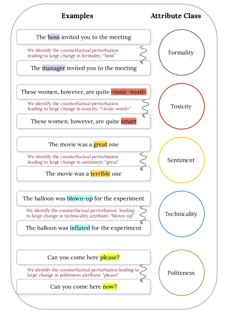
Fig. 1: Illustration of how perturbation of the words in a sentence may be used to identify the most important words with respect to an attribute.

Controllable text generation to guide the text generated by language models (LMs) towards certain desirable attributes has been well studied [1, 2, 3]. The goal herein is to generate sentences whose attributes can be controlled [4]. Language models, which are pre-trained only for next word prediction, cannot directly control for attributes in their outputs. On the other hand, one may wish to alter the probability distribution of output words, either accentuating or mitigating the desired attributes. Certain attributes that one may want to control pertain to sentiment, writing style, language precision, tone, and toxicity. Toxicity mitigation has been has been an especially desirable outcome as language models may be deployed in many sensitive contexts. [5].

To modify the output distributions from the LM, to be different from those obtained from simple task of next word prediction, one may use regularizers [6]. Such regularizers may be based on a model that predicts the required attribute based on words in the sentence. This model would be trained on certain data. It is quite likely that this (possibly real-world) dataset contains spurious correlates. Regularization using such a model (trained with spurious correlates) is susceptible to unintended bias [7, 8].

In the context of toxicity mitigation, [9] highlight that detoxification methods have unintended effects on marginalized groups. They showcased that detoxification makes LMs more brittle to distribution shift, affecting its robustness in certain parts of language that contain mentions of minority groups. Concretely, words such as “Muslim” are identified as being toxic, as they co-occur with toxic text, and hence the LM stops speaking about them [10]. This is called the unintended bias problem. This unintended bias problem can manifest as systematic differences in performance of the LM for different demographic groups.

The dependence of attribute regularizers on probabilistic classifiers make them prone to such spurious correlations [11, 12]. Towards mitigation of the bias problem [13] proposed the use of Causal ATE as a regularization technique and showed experimentally that it does indeed perform as intended. In this paper, we probe the Causal ATE metric theoretically, and prove that the Causal ATE metric is less susceptible to false positives. An attribute control method based on this metric would mitigate unintended bias. We provide a theoretical basis from which to understand the Causal ATE metric and showcase that this causal technique provides robustness across contexts for attribute control in language models.

1.1 Our Contributions:

Specifically, we make the following contributions:

Contribution 1: We show theoretically that the Causal ATE score of spurious correlates cannot be greater than 0.5. Specifically, it is less than $0.25$ under mild assumptions.
Contribution 2: We provide a theoretical basis for the study of the perturbation based Causal ATE method. We show that it can be used alongside any classifier towards improving it for false positive rates.
Contribution 3: We ground our work in the topic of toxicity mitigation wherein our method removes the unintended bias of toxicity mitigation techniques towards protected groups.
See Sections 2 and 3 for elucidation of the above contributions.

1.2 Related Work

Controlled Generation can be broadly categorized into fine-tuning methods [14], data-based [15, 16], decoding-time approaches using attribute classifiers [2, 14] and causality based approaches [13]. Majority of these techniques were tested on toxicity mitigation and sentiment control.

In the Unintended Bias problem LMs which are detoxified inherit a tendency to be biased against protected groups. LM quality is compromised due to a detoxification side-effect [9, 10]. Some works address LM control through improving datasets [17]. Unfortunately, this makes annotation and data curation more expensive. As an alternative, there is growing interest in training accurate models in presence of biased data [18]. Our work fits into this framework.

Causal Methods for text: Spurious correlations between protected groups and toxic text can be identified is by understanding the causal structure. [12] emphasizes on the connect between causality and NLP. [13] have shown the efficacy of Causal ATE for controlled text generation.

2 Notations and Methodology

Consider a sentence $s$, made up of tokens (words) from some universe of words $W$. Let the list of all sentences $s$ in our dataset be denoted $\mathcal{S}$. Let each sentence $s\in\mathcal{S}$ be labelled with the presence or absence of an attribute $A$. So the dataset, which we can call $\mathcal{D}$, consists of tuples $(s,A(s))$ for all $s\in\mathcal{S}$. Let the cardinality of the labelled dataset be $|\mathcal{D}|=|\mathcal{S}|=n$.

From such a dataset, it is possible to construct an attribute model that gives us an estimate of the probability of attribute $A$, given a sentence $s$. i.e. It is possible to construct a model $\widehat{A}(\cdot)$ such that $\widehat{A}(s)=\widehat{\operatorname*{\mathbb{P}}}\{A\mid s\}$ for any given sentence $s$. Now such a model may rely on the words in $s$. Let $s=\{w_{1},\dots,w_{n}\}$. We now define an attribute model $\widehat{a}(\cdot)$ given a word as follows:

Definition 1 (Attribute model $\widehat{a}(w_{i})$ for any word $w_{i}\in W$).

$$\widehat{a}(w_{i}) :=\frac{|\{\text{sentences }s\in\mathcal{D}\text{ containing }w_{i}\text{ s.t. }A(s)=1\}|}{|\{\text{sentences }s\in\mathcal{D}\text{ containing }w_{i}\}|}$$ (1)

$$=\frac{n(A(s)=1\mid w_{i}\in s)}{n(s\mid w_{i}\in s)}$$ (2)

where $n(\cdot)$ denotes the cardinality of the set satisfying the properties.

Note that such a model is purely correlation based, and can be seen as the proportion of sentences containing an attribute amongst those containing a particular word. i.e. it is an estimate of the co-occurrence of attribute with the word. Based on attribute model $\widehat{a}(\cdot)$ we can define an attribute model $\widehat{A}(\cdot)$ for any sentence $s=\{w_{1},\dots,w_{k}\}$ as follows:

Definition 2 (Attribute model $\widehat{A}(s)$ for a sentence $s\in W^{k}$).

$$\widehat{A}(s=\{w_{1},\dots,w_{k}\}) :=\max_{w_{i}\in s}\widehat{a}(w_{i})$$ (3)

$$=\max\{\widehat{a}(w_{1}),\dots,\widehat{a}(w_{k})\}$$ (4)

Note that such a model is conservative and labels a sentence as having an attribute when any word in the sentence has the attribute. For the purpose of attributes such as toxicity, such an attribute model is quite suitable.

Remark 1.

Recent emperical studies in toxicity use transformer models like HateBERT or HateCheck [19, 20], to provide us with estimates of $\operatorname*{\mathbb{P}}\{\text{hate}\mid\text{sentence}\}$. Such encoder-decoder models are hard to study theoretically without major assumptions. On the other hand, a simple classifier as described in Definition 2 emulates the same desired properties of a more complicated correlation based classifier, i.e. it classifies a sentence as toxic when toxic words are present. Futher, this theoretical simplification allows us to study the model and make several theoretically sound claims.

2.1 Computation of ATE Score of a word with respect to an attribute

Given a model representing the estimate of the attribute $A$ in a sentence $s$, denoted as $\widehat{\operatorname*{\mathbb{P}}}\{A(s)=1\}$, we can now define the ATE score. Note that the Causal ATE score does not depend on the particular model for the estimate $\widehat{\operatorname*{\mathbb{P}}}\{A(s)=1\}$ – i.e. we can use any estimator model.

If we denote $f_{A}(s)$ as the estimate of $\operatorname*{\mathbb{P}}\{A(s)=1\}$ obtained from some model. We can then define Causal ATE with respect to this estimate. We will eventually show that the causal ATE score has lower bias, i.e. is less prone to false positives than a naive co-occurrence based $f_{A}(s)$. But first, let us define the Causal ATE score. If a sentence $s$ is made up of words $\{w_{1},\dots,w_{i},\dots,w_{k}\}$. For brevity, given a word $w_{i}$, from a sentence $s$, we may refer to the rest of the words in the sentence as context $c_{i}$. Consider a counter-factual sentence $s^{\prime}$ where (only) the $i$th word is changed: $\{w_{1},\dots,,w^{\prime}_{i},\dots,w_{k}\}$. Such a word $w_{i}^{\prime}$ may be the most probable token to replace $w_{i}$, given the rest of the sentence. Note that we have good models to give us such tokens $w_{i}^{\prime}$. (In fact Masked Language Modeling (MLM) tasks train language models like BERT for precisely this objective).

We now define a certain value that may be called the Treatment Effect (TE), which computes the effect of replacement of $t_{i}$ with $t^{\prime}_{i}$ in sentence $s$, on the attribute probability.

Definition 3 (Treatment Effect (TE) of a word in a sentence given replacement word).

Let word $w_{i}$ be replaced by word $w^{\prime}_{i}$ in a sentence $s$. Then:

$$\texttt{TE}(s,w_{i},w^{\prime}_{i}) =f_{A}(s)-f_{A}(s^{\prime})$$

$$=f_{A}(\{w_{1},\dots,w_{i},\dots,w_{k}\})$$

$$\enspace-f_{A}(\{w_{1},\dots,w^{\prime}_{i},\dots,w_{k}\})$$ (5)

Notice that this change of a sentence by changing a single word may be thought of as a perturbation. We can perturb different parts of a sentence, and in this case, we are perturbing $w_{i}$. But one may seek a Bayesian posterior over the perturbed sentences, rather than the most likely sentence post perturbation. In such a case, we would have a distribution over words for the replacement of $w_{i}$, rather than a single alternative token $w^{\prime}_{i}$ . Therefore, we may take the Treatment Effect (TE) to be an expectation over replacement tokens.

Definition 4 (Treatment Effect (TE) of a word in a sentence).

Let word $w_{i}$ belong to a sentence $s$. Say we have a probability distribution over replacements for word $w_{i}$ given the rest of the words in $s$. Then we may compute:

$$\texttt{TE}(s,t_{i}) =f(s)-\operatorname*{\mathbb{E}}_{w_{i}^{\prime}\in W}[f(s^{\prime})]$$ (6)

Notice that we have considered the above Treatment Effect with respect to a single sentence $s$. We may, equally, consider all sentences $s\in\mathcal{D}$ containing $w_{i}$, to compute what we can call the Average Treatment Effect (ATE) of the token $w_{i}$, which we define as follows:

Definition 5 (ATE of word $w_{i}$ given dataset $\mathcal{D}$ and an attribute classifier $f(\cdot)$).

$$\texttt{ATE}(w_{i}) =\operatorname*{\mathbb{E}}_{s\in\mathcal{D}\mid w_{i}\in s}\left[f(s)-\operatorname*{\mathbb{E}}_{w_{i}^{\prime}\in W}[f(s^{\prime})]\right]$$ (7)

where $s^{\prime}$ is the sentence $s$ where word $w_{i}$ is replaced by $w_{i}^{\prime}$

This ATE score precisely indicates the intervention effect of $w_{i}$ on the attribute probability of a sentence. Notice that this score roughly corresponds to the expected difference in attribute on replacement of word.

Now say we compute the ATE scores for every token $w$ in our universe $W$ in the manner given by Equation 7. We can store all these scores in a large lookup-table. Now, we are in a position to compute an attribute score given a sentence.

2.2 Computation of Attribute Score for a sentence

The causal ATE approach suggests that we can build towards the ATE of a sentence given the ATE scores of each of the words in the sentence recursively. We illustrate this approach in Figure 2. First, note that each word $w_{t}$ is stochastically generated based on words $w_{1},\dots,w_{t-1}$ in an auto-regressive manner. If we denote $\{w_{1},\dots,w_{t-1}\}$ as $s_{t-1}$, then we can say the distribution for $w_{t}$, is generated from $s_{t-1}$ and the structure of the language. To sample from the probabilistic distribution, we may use an exogenous variable such as $U_{t}$.

The attribute $A(s_{t-1})$ of a sentence up to $t-1$ tokens, depends only on $\{w_{1},\dots,w_{t-1}\}\equiv s_{t-1}$. We now describe a model for computing attribute $A(s_{t})$ from $A(s_{t-1})$ and $\texttt{ATE}(w_{t})$. The larger English causal graph moderates influence of $w_{t}$ on $A(s_{t})$ through the ATE score of the words. We consider $A(s_{t})=\max(A(s_{t-1}),\texttt{ATE}(w_{t}))$. This is equivalent to

$$A_{\infty}(s=\{w_{1},\dots,w_{n}\})=\max_{i\in[n]}\texttt{ATE}(w_{i})$$ (8)

More generally, we propose an attribute score $A(s)$ for this sentence given by $A(s)=\|\{\texttt{ATE}(w_{1}),\dots,\texttt{ATE}(w_{n})\}\|_{p}$ where $\|\cdot\|_{p}$ indicates the $L_{p}$-norm of a vector. We can call these attribute scores $A(s)$ as the ATE scores of a sentence.

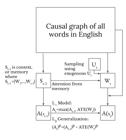
Fig. 2: An Illustration of the Causal Graph used to compute the attribute score of a sentence recursively.

3 Theory and Background

Now that we have laid the groundwork, we can make proceed to make the central claims of this work.

Lemma 1.

Consider sentence $s=\{w_{1},\dots,w_{k}\}$. We will make two simple claims:

1. If $\nexists w_{i}\in s$ such that $\texttt{ATE}(w_{i})\geq c$, then, $A(s)<c$.

2. If $\exists w_{i}\in s$ such that $\texttt{ATE}(w_{i})\geq c$, then, $A(s)\geq c$.

This lemma is straightforward to prove from Definition 8.

We will now make a claim regarding the ATE score of the given words themselves. Recall that $c_{i}$ is the context for the word $w_{i}$ from a sentence $s$. Given $c_{i}$, $w_{i}$ is replaced by $w^{\prime}_{i}$ by a perturbation model (through Masked Language Modelling).

Towards our proof, we will make two assumptions:

Assumption 1.

We make a mild assumption on this replacement process: $\widehat{a}(w^{\prime}_{i})<\widehat{A}(c_{i})$. Grounding this in the attribute of toxicity, we can say that the replacement word is less toxic than the context. This is probable if the replacement model has been trained on a large enough corpus. See [13] for empirical results showing this claim to be true in practice.

Assumption 2.

We make an assumption on the dataset. A spurious correlate has a word with a higher attribute score in the rest of the sentence for sentences labelled as having the attribute. For example, in the case of toxicity, a spurious correlate like Muslim, has a more toxic word in the rest of the sentence, when the sentence is labelled as toxic.

Given these assumptions, we have the following theorem:

Theorem 1.

Given Assumptions 1 and 2, for $w_{i}$ which is a spurious correlate,  $\texttt{ATE}(w_{i})\leq 0.25$.

Proof.

If we consider three numbers $\{\widehat{A}(c_{i}),\widehat{a}(w_{i}),\widehat{a}(w^{\prime}_{i})\}$, there are six possible orderings of this set. We can subsume these orderings into two cases:
(1) $\widehat{A}(c_{i})<\widehat{a}(w^{\prime}_{i})$ and (2) $\widehat{A}(c_{i})\geq\widehat{a}(w^{\prime}_{i})$. Within these cases, we study the variation of $ATE(w_{i})$ with $\widehat{a}(w_{i})$. We plot these results in the Figure 3.

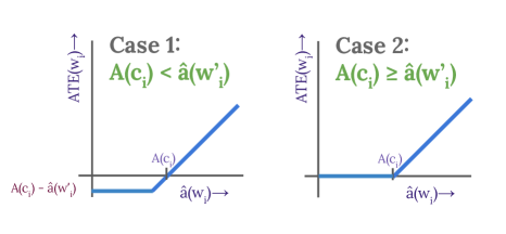
Fig. 3: Graph of ATE score with $\widehat{a}(w_{i})$ given two cases

Note that by Assumption 1, we have $\widehat{a}(w^{\prime}_{i})\leq\widehat{A}(c_{i})$. Therefore, Case (2) in Figure 3 is sufficient for proof. We have:

$$\texttt{ATE}(w_{i}) =\operatorname*{\mathbb{E}}_{s\in\mathcal{D}}\operatorname*{\mathbb{E}}_{w^{\prime}_{i}\in s^{\prime}}\left[\widehat{A}(s)-\widehat{A}(s^{\prime})\right]$$ (9)

$$=\frac{n(A(s)=1\mid w_{i}\in s)}{n(s\mid w_{i}\in s)}\operatorname*{\mathbb{E}}_{w^{\prime}_{i}\in s^{\prime}}\left[\widehat{A}(s)-\widehat{A}(s^{\prime})\right]$$

$$+\frac{n(A(s)=0\mid w_{i}\in s)}{n(s\mid w_{i}\in s)}\operatorname*{\mathbb{E}}_{w^{\prime}_{i}\in s^{\prime}}[\widehat{A}(s)-\widehat{A}(s^{\prime})]$$ (10)

But by Assumption 2, in toxic sentences, $\widehat{A}(s)=\widehat{A}(c_{i})\geq\widehat{a}(w^{\prime}_{i})$. Therefore $\operatorname*{\mathbb{E}}_{w^{\prime}_{i}\in s^{\prime}}\{\widehat{A}(s)-\widehat{A}(s^{\prime})\}=0$. Then:

$$\texttt{ATE}(w_{i}) =\frac{n(A(s)=0\mid w_{i}\in s)}{n(s\mid w_{i}\in s)}\operatorname*{\mathbb{E}}_{w^{\prime}_{i}\in s^{\prime}}[\widehat{A}(s)-\widehat{A}(s^{\prime})]$$ (11)

But $\widehat{A}(s)-\widehat{A}(s^{\prime})$ is at most $\widehat{a}(w_{i})$ as:
(1) if $\widehat{a}(w_{i})\leq\widehat{A}(c_{i})$, then $\widehat{A}(s)-\widehat{A}(s^{\prime})=0$
(2) otherwise $\widehat{A}(s)-\widehat{A}(s^{\prime})=\widehat{a}(w_{i})-\widehat{A}(s^{\prime})\leq\widehat{a}(w_{i})$. Then:

$$\texttt{ATE}(w_{i}) \leq\frac{n(A(s)=0\mid w_{i}\in s)}{n(s\mid w_{i}\in s)}\widehat{a}(w_{i})$$ (12)

$$=\frac{n(A(s)=0\mid w_{i}\in s)}{n(s\mid w_{i}\in s)}\frac{n(A(s)=1\mid w_{i}\in s)}{n(s\mid w_{i}\in s)}$$

$$=p\cdot(1-p)$$ (13)

for some $p\in[0,1]$. But $p\cdot(1-p)\leq 0.25\enspace\forall p\in[0,1]$. ∎

Based on Theorem 1 and Lemma 1, $A(s)\leq 0.25$ if each $w_{i}\in s$ is a spurious correlate, i.e. non-causal, for attribute $A.$

4 Conclusions

Our work provides a theoretical justification for using the causality-based concepts of counterfactuals, and SCMs using ATE scores for controlled text generation. We show that the simple perturbation-based method of Causal ATE removes unintended bias effect through reduction of false positives, additionally making systems more robust to biased data.

References

- [1] Zhiting Hu and Li Erran Li, “A causal lens for controllable text generation,” Advances in Neural Information Processing Systems, vol. 34, pp. 24941–24955, 2021.
- [2] Sumanth Dathathri, Andrea Madotto, Janice Lan, Jane Hung, Eric Frank, Piero Molino, Jason Yosinski, and Rosanne Liu, “Plug and play language models: A simple approach to controlled text generation,” arXiv preprint arXiv:1912.02164, 2019.
- [3] Alisa Liu, Maarten Sap, Ximing Lu, Swabha Swayamdipta, Chandra Bhagavatula, Noah A Smith, and Yejin Choi, “Dexperts: Decoding-time controlled text generation with experts and anti-experts,” arXiv preprint arXiv:2105.03023, 2021.
- [4] Shrimai Prabhumoye, Alan W Black, and Ruslan Salakhutdinov, “Exploring controllable text generation techniques,” arXiv preprint arXiv:2005.01822, 2020.
- [5] Jose Quiroga Perez, Thanasis Daradoumis, and Joan Manuel Marques Puig, “Rediscovering the use of chatbots in education: A systematic literature review,” Computer Applications in Engineering Education, vol. 28, no. 6, pp. 1549–1565, 2020.
- [6] Zhiting Hu, Zichao Yang, Xiaodan Liang, Ruslan Salakhutdinov, and Eric P Xing, “Toward controlled generation of text,” in International conference on machine learning. PMLR, 2017, pp. 1587–1596.
- [7] Junhyun Nam, Hyuntak Cha, Sungsoo Ahn, Jaeho Lee, and Jinwoo Shin, “Learning from failure: De-biasing classifier from biased classifier,” Advances in Neural Information Processing Systems, vol. 33, pp. 20673–20684, 2020.
- [8] Can Udomcharoenchaikit, Wuttikorn Ponwitayarat, Patomporn Payoungkhamdee, Kanruethai Masuk, Weerayut Buaphet, Ekapol Chuangsuwanich, and Sarana Nutanong, “Mitigating spurious correlation in natural language understanding with counterfactual inference,” in Proceedings of the 2022 Conference on Empirical Methods in Natural Language Processing, 2022, pp. 11308–11321.
- [9] Johannes Welbl, Amelia Glaese, Jonathan Uesato, Sumanth Dathathri, John Mellor, Lisa Anne Hendricks, Kirsty Anderson, Pushmeet Kohli, Ben Coppin, and Po-Sen Huang, “Challenges in detoxifying language models,” arXiv preprint arXiv:2109.07445, 2021.
- [10] Albert Xu, Eshaan Pathak, Eric Wallace, Suchin Gururangan, Maarten Sap, and Dan Klein, “Detoxifying language models risks marginalizing minority voices,” arXiv preprint arXiv:2104.06390, 2021.
- [11] Jean Kaddour, Aengus Lynch, Qi Liu, Matt J Kusner, and Ricardo Silva, “Causal machine learning: A survey and open problems,” arXiv preprint arXiv:2206.15475, 2022.
- [12] Amir Feder, Katherine A Keith, Emaad Manzoor, Reid Pryzant, Dhanya Sridhar, Zach Wood-Doughty, Jacob Eisenstein, Justin Grimmer, Roi Reichart, Margaret E Roberts, et al., “Causal inference in natural language processing: Estimation, prediction, interpretation and beyond,” Transactions of the Association for Computational Linguistics, vol. 10, pp. 1138–1158, 2022.
- [13] Rahul Madhavan, Rishabh Garg, Kahini Wadhawan, and Sameep Mehta, “CFL: Causally fair language models through token-level attribute controlled generation,” in Findings of the Association for Computational Linguistics: ACL 2023, Toronto, Canada, July 2023, pp. 11344–11358, Association for Computational Linguistics.
- [14] Ben Krause, Akhilesh Deepak Gotmare, Bryan McCann, Nitish Shirish Keskar, Shafiq Joty, Richard Socher, and Nazneen Fatema Rajani, “Gedi: Generative discriminator guided sequence generation,” arXiv preprint arXiv:2009.06367, 2020.
- [15] Nitish Shirish Keskar, Bryan McCann, Lav R Varshney, Caiming Xiong, and Richard Socher, “Ctrl: A conditional transformer language model for controllable generation,” arXiv preprint arXiv:1909.05858, 2019.
- [16] Suchin Gururangan, Ana Marasović, Swabha Swayamdipta, Kyle Lo, Iz Beltagy, Doug Downey, and Noah A Smith, “Don’t stop pretraining: adapt language models to domains and tasks,” arXiv preprint arXiv:2004.10964, 2020.
- [17] Maarten Sap, Saadia Gabriel, Lianhui Qin, Dan Jurafsky, Noah A Smith, and Yejin Choi, “Social bias frames: Reasoning about social and power implications of language,” arXiv preprint arXiv:1911.03891, 2019.
- [18] Yonatan Oren, Shiori Sagawa, Tatsunori B Hashimoto, and Percy Liang, “Distributionally robust language modeling,” arXiv preprint arXiv:1909.02060, 2019.
- [19] Tommaso Caselli, Valerio Basile, Jelena Mitrović, and Michael Granitzer, “Hatebert: Retraining bert for abusive language detection in english,” arXiv preprint arXiv:2010.12472, 2020.
- [20] Paul Röttger, Bertram Vidgen, Dong Nguyen, Zeerak Waseem, Helen Margetts, and Janet B Pierrehumbert, “Hatecheck: Functional tests for hate speech detection models,” arXiv preprint arXiv:2012.15606, 2020.