The general solutions for a non-isospectral integrable TD hierarchy via the inverse scattering transform

Hongyi Zhang¹, Yufeng Zhang¹, Binlu Feng^2∗

¹School of Mathematics, China University of Mining and Technology, Xuzhou, Jiangsu, 221116, People’s Republic of China.
²School of Mathematics and Information Sciences, Weifang University, Weifang,Shandong, 261061, People’s Republic of China.

Keywords

Exact solution; Non-isospectral TD hierarchy; Inverse scattering transform

1. Introduction

The inverse scattering transform (IST) was initially proposed by Gardner et al. in 1967 [1], who successfully applied them to the Korteweg-de Vries (KdV) equation. The classical IST methods are generally studied using the Gel’fand-Levitan-Marchenko integral equation as a foundation. In 1984, Zakharov et al. appropriately simplified the IST method by issuing the Riemann-Hilbert (RH) formula [2]. Subsequently, more and more researchers have utilized this method to obtain the soliton solutions for nonlinear evolution equations [3, 4, 5, 6, 7, 8, 9, 10, 11]. In general, there are two kinds of evolution equations associated with the same spectral problems, called isospectral hierarchy and non-isospectral hierarchy, respectively. The isospectral equations mainly describe solitary waves in lossless homogeneous media. These equations describe situations where the spectral parameters remain constant with time. In recent years, the derivation, reduction and application of non-isospectral equations have been well developed [12, 13, 14, 15]. In contrast, the non-isospectral equations arise from the spectral problem with time-dependent spectral parameter $\lambda$ [16, 17, 18, 19, 20, 21], and IST can be efficiently applied to solve these equations, and their solutions prove the existence of solitary waves in certain types of inhomogeneous media [22, 23, 24]. In addition, the search for exact solutions to nonisospectral equations is of great importance mathematically due to the involvement of time-dependent spectral parameters. Previous discussions have addressed some issues related to seeking exact solutions for nonisospectral equations. Additionally, some non-isospectral equations have been successfully solved by using IST method [23, 24, 25].

The TD hierarchy associated with spectral problem

$$\Psi_{x}=\left(\begin{array}[]{cc}-\lambda+s&q\\ r&\lambda\end{array}\right)\Psi,\quad\Psi=(\Psi_{1},\Psi_{2})^{T},$$ (1.1)

is one of the integrable hierarchies series (ranging from the TA hierarchy to the TD hierarchy) proposed and named by Tu [28, 29]. Spectrum problem (1.1) is equivalently to spectral problem [30]

$$\Psi_{x}=\left(\begin{array}[]{cc}i\lambda+u&v\\ v&-i\lambda-u\end{array}\right)\Psi,\quad\Psi=(\Psi_{1},\Psi_{2})^{T}.$$ (1.2)

Zhu [32, 33] utilized (1.2) to get the so-called TD equation:

$$\begin{cases}iu_{t}+\left(\frac{v_{xx}}{4v}+u^{2}-\frac{v^{2}}{2}\right)_{x}=0,\\ iv_{t}+u_{x}v+2uv_{x}=0.\end{cases}$$ (1.3)

In the paper, by choosing new expressions for the time part of the Lax pair, through a non-isospectral zero-curvature equation, a new non-isospectral integrable TD system (see below (2.13)) is worked out, meanwhile, the TD equation (1.3) is only its special case in isospectral case. In Section 2, we depict the derivation of the non-isospectral TD hierarchy. In Section 3, we obtain the general solutions of the non-isospectral integrable TD hierarchy through the IST method. Based on our paper [38], we analyze dynamic behaviors of the soliton solutions.

2. A non-isospectral integrable TD hierarchy

Consider the TD spectral problem [30]

$$\Psi_{x}=M\Psi,\quad M=\left(\begin{array}[]{cc}i\lambda+u&v\\ v&-i\lambda-u\end{array}\right),\quad\Psi=(\Psi_{1},\Psi_{2})$$ (2.1)

and the time evolution introduced by us:

$$\Psi_{t}=N\Psi,\quad N=\left(\begin{array}[]{cc}A&B+C\\ B-C&-A\end{array}\right),$$ (2.2)

where $u(x,t)$ and $v(x,t)$ are potential functions, $\lambda$ is a spectral parameter, and $A=\sum_{i=0}^{n+2}A_{i}\lambda^{n+2-i}$, $B=\sum_{i=0}^{n+1}B_{i}\lambda^{n+1-i}$, $C=\sum_{i=0}^{n}C_{i}\lambda^{n-i}$. We assume that $u(x,t)$ and $v(x,t)$ are smooth functions of $x$ and $t$; and their derivatives of any order with respect to $x$ vanish rapidly as $x\rightarrow\infty$. The compatibility condition reads

$$M_{t}-N_{x}+[M,N]=0,$$ (2.3)

expanding the matrices $M$ and $N$ gives

$$\begin{cases}i\lambda_{t}+u_{t}-A_{x}-2vC=0,\\ v_{t}-B_{x}-C_{x}-2vA+2(i\lambda+u)(B+C)=0,\\ v_{t}-B_{x}+C_{x}+2vA-2(i\lambda+u)(B-C)=0.\end{cases}$$ (2.4)

Simplifying the above equation, we get

$$i\lambda_{t}+u_{t}-A_{x}-2vC=0,$$ (2.5)

$$v_{t}-B_{x}+2(i\lambda+u)C=0,$$ (2.6)

$$C_{x}+2vA-2(i\lambda+u)B=0.$$ (2.7)

Comparing the coefficients of $\lambda^{l}(l=0,1,\cdots n+1)$ in (2.5) and (2.6) respectively, we get

$$\begin{cases}u_{t}-A_{n+2,x}-2vC_{n}=0,\\ -A_{i+2,x}-2vC_{i}=0,\\ i\lambda_{t}-A_{1,x}\lambda^{n+1}-A_{0,x}\lambda^{n+2}=0,\\ v_{t}-B_{n+1,x}+2uC_{n}=0,\\ -B_{i+1,x}+2uC_{i}+2iC_{i+1}=0,\\ -B_{0,x}+2iC_{0}=0.\end{cases}$$ (2.8)

Then we consider the coefficients of $\lambda^{l}(l=0,1,\cdots n+2)$ in (2.7), to get

$$\begin{cases}C_{n,x}+2vA_{n+2}-2uB_{n+1}=0,\\ C_{i,x}+2vA_{i+2}-2iB_{i+2}-2uB_{i+1}=0,\\ 2vA_{1}-2iB_{1}-2uB_{0}=0,\\ 2vA_{0}-2iB_{0}=0.\end{cases}$$ (2.9)

In contrast to the isospectral case, the nonisospectral case involves spectral parameters that depend on time [16, 17, 18, 19, 20, 21]. We choose $\lambda_{t}=\lambda^{n+1}$ here, and take the initial values
$~{}~{}~{}~{}~{}~{}~{}~{}~{}~{}~{}~{}~{}~{}~{}~{}~{}~{}~{}~{}~{}~{}~{}~{}~{}~{}~{}~{}~{}~{}~{}~{}~{}~{}~{}~{}~{}~{}~{}~{}~{}~{}~{}~{}~{}~{}~{}~{}~{}~{}~{}~{}~{}~{}~{}~{}A_{0}=0$,  $B_{0}=0$,  $C_{0}=0$,
which can be obtained by equations (2.8) and (2.9)
$~{}~{}~{}~{}~{}~{}~{}~{}~{}~{}~{}~{}~{}~{}~{}~{}~{}~{}~{}~{}~{}~{}~{}~{}~{}~{}~{}~{}~{}~{}~{}~{}~{}~{}~{}~{}~{}~{}~{}A_{1}=ix$,  $B_{1}=xv$,  $C_{1}=-\frac{i}{2}(v+xv_{x})$,  $A_{2}=0$,  $B_{2}=ixuv$.
For $i=0,\cdots n-1$, from equations (2.8) and (2.9) we can get

$$\begin{cases}-A_{i+2,x}-2vC_{i}=0,\\ -B_{i+1,x}+2uC_{i}+2iC_{i+1}=0,\\ C_{i,x}+2vA_{i+2}-2iB_{i+2}-2uB_{i+1}=0.\end{cases}$$ (2.10)

From equation (2.10), we get the following recurrence relation

$$\left(\begin{array}[]{c}B_{i+2}\\ C_{i+1}\end{array}\right)=\left(\begin{array}[]{cc}iu&iv\partial^{-1}(2v)-\frac{i}{2}\partial\\ -\frac{i}{2}\partial&iu\end{array}\right)\left(\begin{array}[]{c}B_{i+1}\\ C_{i}\end{array}\right)=L\left(\begin{array}[]{c}B_{i+1}\\ C_{i}\end{array}\right),$$ (2.11)

where
$~{}~{}~{}~{}~{}~{}~{}~{}~{}~{}~{}~{}~{}~{}~{}~{}~{}~{}~{}~{}~{}~{}~{}~{}~{}~{}~{}~{}~{}~{}~{}~{}~{}~{}~{}~{}~{}~{}~{}~{}~{}~{}~{}~{}~{}~{}~{}L=\left(\begin{array}[]{cc}iu&iv\partial^{-1}(2v)-\frac{i}{2}\partial\\ -\frac{i}{2}\partial&iu\end{array}\right)$.
From the values of $B_{i}$ and $C_{i}$ we can get the value of $A_{i}$. For $n=0$, we get $A_{1}=ix$, $A_{2}=xu$ by (2.9); For $n\geq 1$, by equations (2.8) and (2.9) we obtain $A_{i+2}=\partial^{-1}(-2vC_{i})$ $(i=0,1,\cdots n-1)$ and $A_{n+2}=\frac{2uB_{n+1}-C_{n,x}}{2v}$ respectively. Finally, we obtain the TD non-isospectral equation

$$\begin{cases}u_{t}=2vC_{n}+\left(\frac{2uB_{n+1}-C_{n,x}}{2v}\right)_{x},\\ v_{t}=B_{n+1,x}-2uC_{n},\end{cases}$$ (2.12)

when $n=1$, (2.12) reduced to:

$$\begin{cases}u_{t}=-i\left(v^{2}+xvv_{x}\right)+\left(\frac{2iu^{2}vx+\frac{i}{2}\left(v+xv_{x}\right)_{x}}{2v}\right)_{x},\\ v_{t}=B_{2,x}-2uC_{1}=2iu\left(v+xv_{x}\right)+ixu_{x}v.\end{cases}$$ (2.13)

$\mathbf{Remark~{}2.1.}$ Setting $\lambda_{t}=0$ in (2.1), by the same method as in the previous non-isospectral equations, we get

$$\begin{cases}u_{t}=2vC_{n}+\left(\frac{2uB_{n+1}-C_{n,x}}{2v}\right)_{x},\\ v_{t}=B_{n+1,x}-2uC_{n}.\end{cases}$$ (2.14)

with

$$\begin{cases}B_{1}=uvA_{0}-ivA_{1},C_{0}=-\frac{1}{2}A_{0}v_{x},\\ \left(\begin{array}[]{c}B_{i+2}\\ C_{i+1}\end{array}\right)=L\left(\begin{array}[]{c}B_{i+1}\\ C_{i}\end{array}\right),~{}(i=0,\cdots,n)\end{cases}$$ (2.15)

where $A_{0},A_{1}$ are arbitrary constants. In this case, the isospectral hierarchy (2.14) is equivalent to the isospectral TD hierarchy [29, 30].

Moreover, we note that (2.14) becomes the TD equation (1.3) when $A_{0}=0,A_{1}=i$ and $n=1$.

3. General solution of the non-isospectral TD hierarchy

In this section, we will give the direct scattering problem and the time evolution of the scattering data, which holds for the entire hierarchy. Finally, by using the classical inverse scattering transform, we obtain the N-soliton solution of the entire non-isospectral TD hierarchy.

3.1. The direct scattering problem

$\mathbf{Lemma~{}3.1.}$ If potential $(u(x),v(x))^{T}$ satisfies

$$\int_{-\infty}^{\infty}|x^{j}u(x)|dx<+\infty,~{}~{}\int_{-\infty}^{\infty}|x^{j}v(x)|dx<+\infty~{}~{}(j=0,1),$$ (3.1)

then the spectral problem (2.1) has a group of Jost solutions $\phi(x;\lambda)$, $\widetilde{\phi}(x;\lambda)$, $\psi(x;\lambda)$ and $\widetilde{\psi}(x;\lambda)$ which are bounded for all values of $x$, and also have the following asymptotic behaviors:
when $x\rightarrow+\infty$,

$$\begin{array}[]{l}\phi(x;\lambda)=\left(\begin{array}[]{c}\phi_{1}\\ \phi_{2}\end{array}\right)\rightarrow\left(\begin{array}[]{c}1\\ 0\end{array}\right)e^{i\lambda x},~{}~{}~{}\widetilde{\phi}(x;\lambda)=\left(\begin{array}[]{c}\widetilde{\phi}_{1}\\ \widetilde{\phi}_{2}\end{array}\right)\rightarrow\left(\begin{array}[]{c}0\\ 1\end{array}\right)e^{-i\lambda x},\\ \phi_{x}(x;\lambda)\rightarrow i\lambda\left(\begin{array}[]{c}1\\ 0\end{array}\right)e^{i\lambda x},~{}~{}~{}\widetilde{\phi}_{x}(x;\lambda)\rightarrow-i\lambda\left(\begin{array}[]{c}0\\ 1\end{array}\right)e^{-i\lambda x},\\ \phi_{\lambda}(x;\lambda)\rightarrow ix\left(\begin{array}[]{c}1\\ 0\end{array}\right)e^{i\lambda x},~{}~{}~{}\widetilde{\phi}_{\lambda}(x;\lambda)\rightarrow-ix\left(\begin{array}[]{c}0\\ 1\end{array}\right)e^{-i\lambda x},\end{array}$$ (3.2)

and when $x\rightarrow-\infty$,

$$\begin{array}[]{l}\psi(x;\lambda)=\left(\begin{array}[]{c}\psi_{1}\\ \psi_{2}\end{array}\right)\rightarrow\left(\begin{array}[]{c}0\\ 1\end{array}\right)e^{-i\lambda x},~{}~{}~{}\widetilde{\psi}(x;\lambda)=\left(\begin{array}[]{c}\widetilde{\psi}_{1}\\ \widetilde{\psi}_{2}\end{array}\right)\rightarrow\left(\begin{array}[]{c}1\\ 0\end{array}\right)e^{i\lambda x},\\ \psi_{x}(x;\lambda)\rightarrow-i\lambda\left(\begin{array}[]{c}0\\ 1\end{array}\right)e^{-i\lambda x},~{}~{}~{}\widetilde{\psi}_{x}(x;\lambda)\rightarrow i\lambda\left(\begin{array}[]{c}1\\ 0\end{array}\right)e^{i\lambda x},\\ \psi_{\lambda}(x;\lambda)\rightarrow-ix\left(\begin{array}[]{c}0\\ 1\end{array}\right)e^{-i\lambda x},~{}~{}~{}\widetilde{\psi}_{\lambda}(x;\lambda)\rightarrow ix\left(\begin{array}[]{c}1\\ 0\end{array}\right)e^{i\lambda x}.\\ \end{array}$$ (3.3)

$\mathbf{Proof}$: A direct calculation gives rise to the conclusion.
$\mathbf{Lemma~{}3.2.}$ When $\lambda\rightarrow\infty$, we have the following asymptotics

$$\begin{array}[]{l}\phi(x;\lambda)\rightarrow\left(\begin{array}[]{c}1\\ 0\end{array}\right)e^{i\lambda x},~{}~{}~{}\widetilde{\phi}(x;\lambda)\rightarrow\left(\begin{array}[]{c}0\\ 1\end{array}\right)e^{-i\lambda x},\\ \psi(x;\lambda)\rightarrow\left(\begin{array}[]{c}0\\ 1\end{array}\right)e^{-i\lambda x},~{}~{}~{}\widetilde{\psi}(x;\lambda)\rightarrow\left(\begin{array}[]{c}1\\ 0\end{array}\right)e^{i\lambda x}.\end{array}$$ (3.4)

$\mathbf{Proof}$. From spectral problem (2.1), we get

$$\left(\begin{array}[]{c}\phi_{1}(x,\lambda)\\ \phi_{2}(x,\lambda)\end{array}\right)_{x}=\left(\begin{array}[]{cc}i\lambda+u&v\\ v&-i\lambda-u\end{array}\right)\left(\begin{array}[]{c}\phi_{1}(x,\lambda)\\ \phi_{2}(x,\lambda)\end{array}\right),$$ (3.5)

and also

$$\phi_{1,x}(x,\lambda)=(i\lambda+u)\phi_{1}(x,\lambda)+v\phi_{2}(x,\lambda),$$ (3.6)

$$\phi_{2,x}(x,\lambda)=v\phi_{1}(x,\lambda)-(i\lambda+u)\phi_{2}(x,\lambda).$$ (3.7)

By (3.6), we get

$$\phi_{2}(x,\lambda)=\frac{\phi_{1,x}(x,\lambda)-(i\lambda+u)\phi_{1}(x,\lambda)}{v}.$$ (3.8)

Substituting (3.8) into (3.7), we obtain that

$$\left(\frac{\phi_{1,x}(x,\lambda)-(i\lambda+u)\phi_{1}(x,\lambda)}{v}\right)_{x}=v\phi_{1}(x,\lambda)-(i\lambda+u)\frac{\phi_{1,x}(x,\lambda)-(i\lambda+u)\phi_{1}(x,\lambda)}{v}.\\$$ (3.9)

Rewriting equation (3.9), one also has

$$\phi_{1,xx}(x,\lambda)-u_{x}\phi_{1}(x,\lambda)-\frac{\phi_{1,x}(x,\lambda)v_{x}}{v}+\frac{(i\lambda+u)\phi_{1}(x,\lambda)v_{x}}{v}-v^{2}\phi_{1}(x,\lambda)+\lambda^{2}\phi_{1}(x,\lambda)-u^{2}\phi_{1}(x,\lambda)-2i\lambda u\phi_{1}(x,\lambda)=0.$$ (3.10)

Let
$~{}~{}~{}~{}~{}~{}~{}~{}~{}~{}~{}~{}~{}~{}~{}~{}~{}~{}~{}~{}~{}~{}~{}~{}~{}~{}~{}~{}~{}~{}~{}~{}~{}~{}~{}~{}~{}~{}~{}~{}~{}~{}~{}~{}~{}~{}~{}~{}~{}~{}~{}~{}~{}~{}~{}\phi_{1}(x,\lambda)=e^{i\lambda x+\widehat{\phi}_{1}(x,\lambda)}$,
where
$~{}~{}~{}~{}~{}~{}~{}~{}~{}~{}~{}~{}~{}~{}~{}~{}~{}~{}~{}~{}~{}~{}~{}~{}~{}~{}~{}~{}~{}~{}~{}~{}~{}~{}~{}~{}~{}~{}~{}~{}~{}~{}~{}~{}~{}~{}~{}~{}~{}~{}~{}~{}~{}\widehat{\phi}_{1}(x,\lambda)=\sum_{i=0}^{+\infty}\frac{a_{i}}{\lambda^{i}}$, $\lambda\rightarrow\infty$.
So we have

$$\phi_{1,x}(x,\lambda)=(i\lambda+\widehat{\phi}_{1,x}(x,\lambda))\phi_{1}(x,\lambda),$$ (3.11)

$$\phi_{1,xx}(x,\lambda)=\widehat{\phi}_{1,xx}(x,\lambda)\phi_{1}(x,\lambda)+(i\lambda+\widehat{\phi}_{1,x}(x,\lambda))^{2}\phi_{1}(x,\lambda),$$ (3.12)

substituting (3.11) and (3.12) into (3.10) yields

$$\widehat{\phi}_{1,xx}(x,\lambda)+\widehat{\phi}_{1,x}^{2}(x,\lambda)+2i\lambda\widehat{\phi}_{1,x}(x,\lambda)-u_{x}-\frac{v_{x}}{v}\widehat{\phi}_{1,x}(x,\lambda)+\frac{u}{v}v_{x}-v^{2}-u^{2}-2i\lambda u=0.$$ (3.13)

By comparing the coefficients of $\lambda^{j}$ $(j=1,\cdots,n)$, we get

$$\begin{cases}a_{0}=-\int_{x}^{+\infty}udx,\\ a_{1,x}=\frac{-iv^{2}}{2}.\end{cases}$$ (3.14)

Therefore, we get

$$\phi_{1}(x,\lambda)=e^{i\lambda x-\int_{x}^{+\infty}(u-\frac{iv^{2}}{2\lambda})dx+o(\lambda^{-2})}.$$ (3.15)

When $\lambda\rightarrow\infty$, we have

$$\phi_{2}(x,\lambda) =\frac{\phi_{1,x}(x,\lambda)-(i\lambda+u)\phi_{1}(x,\lambda)}{v}$$ (3.16)

$$\sim\frac{\left(i\lambda+u-\frac{iv^{2}}{2\lambda}\right)\phi_{1}(x,\lambda)-(i\lambda+u)\phi_{1}(x,\lambda)}{v}$$

$$\sim\frac{-iv}{2\lambda}\phi_{1}(x,\lambda).$$

Similarly, when $\lambda\rightarrow\infty$, we obtain that

$$\begin{cases}\psi_{2}(x,\lambda)=e^{-i\lambda x-\int_{-\infty}^{x}(u+\frac{v^{2}}{2i\lambda})dx+o(\lambda^{-2})},\\ \psi_{1}(x,\lambda)=\frac{iv}{2\lambda}\psi_{2}(x,\lambda),\end{cases}$$ (3.17)

$$\begin{cases}\widetilde{\phi}_{2}(x,\lambda)=e^{-i\lambda x+\int_{x}^{+\infty}(u+\frac{v^{2}}{2i\lambda})dx+o(\lambda^{-2})},\\ \widetilde{\phi}_{1}(x,\lambda)=\frac{iv}{2\lambda}\widetilde{\phi}_{2}(x,\lambda),\end{cases}$$ (3.18)

and

$$\begin{cases}\widetilde{\psi}_{1}(x,\lambda)=e^{i\lambda x+\int_{-\infty}^{x}(u-\frac{iv^{2}}{2\lambda})dx+o(\lambda^{-2})},\\ \widetilde{\psi}_{2}(x,\lambda)=\frac{-iv}{2\lambda}\widetilde{\psi}_{1}(x,\lambda).~{}~{}~{}~{}~{}~{}~{}~{}~{}~{}~{}~{}~{}~{}~{}~{}~{}~{}~{}~{}~{}~{}~{}~{}~{}~{}~{}\Box\end{cases}$$ (3.19)

Define the Wronskian determinant of $\left(\phi(x,\lambda),\widetilde{\phi}(x,\lambda)\right)$ as

$$W(\phi(x,\lambda),\widetilde{\phi}(x,\lambda))=\phi_{1}(x,\lambda)\widetilde{\phi}_{2}(x,\lambda)-\widetilde{\phi}_{1}(x,\lambda)\phi_{2}(x,\lambda),$$ (3.20)

and assume that

$$\begin{cases}\phi(x,\lambda)=a(\lambda)\widetilde{\psi}(x,\lambda)+b(\lambda)\psi(x,\lambda),\\ \widetilde{\phi}(x,\lambda)=-\widetilde{a}(\lambda)\psi(x,\lambda)+\widetilde{b}(\lambda)\widetilde{\psi}(x,\lambda),\end{cases}$$ (3.21)

we have

$$\left(\begin{array}[]{cc}\phi(x,\lambda)&\widetilde{\phi}(x,\lambda)\\ \end{array}\right)=\left(\begin{array}[]{cc}\widetilde{\psi}(x,\lambda)&\psi(x,\lambda)\\ \end{array}\right)\left(\begin{array}[]{cc}a(\lambda)&\widetilde{b}(\lambda)\\ b(\lambda)&-\widetilde{a}(\lambda)\end{array}\right).$$ (3.22)

According to (2.1) and Lemma 3.1, we get

$$a(\lambda)=W(\phi(x;\lambda),\psi(x;\lambda)),~{}~{}\widetilde{a}(\lambda)=W(\widetilde{\phi}(x;\lambda),\widetilde{\psi}(x;\lambda)),$$ (3.23)

$$b(\lambda)=W(\widetilde{\psi}(x;\lambda),\phi(x;\lambda)),~{}~{}\widetilde{b}(\lambda)=W(\widetilde{\phi}(x;\lambda),\psi(x;\lambda)).$$ (3.24)

The solution of spectral problem (2.1) has the following asymptotics:

$$\Psi(x,\lambda)=\left(\widetilde{\psi}(x,\lambda),\psi(x,\lambda)\right)\rightarrow e^{i\lambda x\sigma_{3}},~{}~{}x\rightarrow\infty.$$ (3.25)

Taking the transformation

$$\mu(x,\lambda)=\Psi(x,\lambda)e^{-i\lambda x\sigma_{3}},$$ (3.26)

we have

$$\mu(x,\lambda)\rightarrow I,~{}~{}x\rightarrow\infty.$$ (3.27)

From spectral problem (2.1), we obtain

$$\mu_{x}(x,\lambda)+i\lambda[\mu(x,\lambda),\sigma_{3}]=Q\mu(x,\lambda),$$ (3.28)

where
$~{}~{}~{}~{}~{}~{}~{}~{}~{}~{}~{}~{}~{}~{}~{}~{}~{}~{}~{}~{}~{}~{}~{}~{}~{}~{}~{}~{}~{}~{}~{}~{}~{}~{}~{}~{}~{}~{}~{}~{}~{}~{}~{}~{}~{}~{}~{}~{}~{}~{}~{}~{}~{}~{}~{}~{}~{}~{}Q=\left(\begin{array}[]{cc}u&v\\ v&-u\end{array}\right)$.
Eq. (3.28) can be rewritten in differential form

$$d\left(e^{-i\lambda x\hat{\sigma}_{3}}\mu\right)=e^{-i\lambda x\hat{\sigma}_{3}\mu}[Qdx\mu].$$ (3.29)

Therefore, we get

$$\mu_{-}=I+\int_{-\infty}^{x}e^{i\lambda(x-y)\hat{\sigma}_{3}}[Q\mu_{-}dy].$$ (3.30)

$\mathbf{Lemma~{}3.3.}$ $\mu_{-,1}(x,\lambda)$ and $\mu_{+,2}(x,\lambda)$ are analytical on $Im(\lambda)<0$, $\mu_{+,1}(x,\lambda)$ and $\mu_{-,2}(x,\lambda)$ are analytical on $Im(\lambda)>0$. So that $\phi(x,\lambda)$ and $\psi(x,\lambda)$ are analytical on $Im(\lambda)>0$, $\widetilde{\phi}(x,\lambda)$ and $\widetilde{\psi}(x,\lambda)$ are analytical on $Im(\lambda)<0$.
$\mathbf{Proof.}$ Let $\omega(x,\lambda)=\mu_{-,1}(x,\lambda)$, we have

$$\omega(x,\lambda)=\left(\begin{array}[]{c}1\\ 0\end{array}\right)+\int_{-\infty}^{x}C_{-}(x,\lambda)\omega(y,\lambda)dy,$$ (3.31)

where
$~{}~{}~{}~{}~{}~{}~{}~{}~{}~{}~{}~{}~{}~{}~{}~{}~{}~{}~{}~{}~{}~{}~{}~{}~{}~{}~{}~{}~{}~{}~{}~{}~{}~{}~{}~{}~{}~{}~{}~{}~{}~{}~{}~{}~{}~{}~{}~{}~{}~{}C_{-}(x,\lambda)=diag(1,e^{-2i\lambda(x-y)})Q(y,\lambda)$.
We constructe a Neumann series

$$\omega(x,\lambda)=\sum_{n=1}^{\infty}\omega^{(n)}(x,\lambda),$$ (3.32)

and define the norm of the vector $L^{1}$ as $\|\omega\|=|\omega_{1}|+|\omega_{2}|$. A direct calculation yields the following estimation

$$\|C_{-}\|=\|diag(1,e^{-2i\lambda(x-y)})\|\cdot\|Q\|\leq\left(1+e^{2Im\lambda(x-y)}\right)\cdot(2|u|+2|v|)\leq 4(|u|+|v|).$$ (3.33)

So we have

$$\omega^{0}=\left(\begin{array}[]{c}1\\ 0\end{array}\right),$$ (3.36)

$$\omega^{n+1}(x,\lambda)=\int_{-\infty}^{x}C_{-}(y,z)\omega^{n}(y,\lambda)dy,$$ (3.37)

which indicates

$$\|\omega^{(n+1)}(x,\lambda)\|\leq\int_{-\infty}^{x}\|C_{-}\|\|\omega^{(n)}(y,\lambda)\|dy.$$ (3.38)

Substituting (3.33) into (3.38), it can be obtained that

$$\|\omega^{n+1}(x,\lambda)\|\leq\int_{-\infty}^{x}4(|u|+|v|)\|\omega^{(n)}(y,\lambda)\|dy.$$ (3.39)

We denote
$~{}~{}~{}~{}~{}~{}~{}~{}~{}~{}~{}~{}~{}~{}~{}~{}~{}~{}~{}~{}~{}~{}~{}~{}~{}~{}~{}~{}~{}~{}~{}~{}~{}~{}~{}~{}~{}~{}~{}~{}~{}~{}~{}~{}~{}~{}~{}~{}~{}~{}~{}~{}\rho(x)=\int_{-\infty}^{x}4(|u|+|v|)dy$,
the above integral exists when $u(x)\in L^{1}(R)$, $v(x)\in L^{1}(R)$, for any fixed $x\in R$, we have

$$\rho_{x}(x)=4(|u|+|v|),~{}~{}\|\omega^{(1)}\|\leq\rho(x).$$ (3.40)

By mathematical induction and assuming that $\|\omega^{(n)}(x,\lambda)\|\leq\frac{\rho^{n}(x)}{n!}$, we obtain that

$$\|\omega^{(n+1)}(x,\lambda)\|\leq\int_{-\infty}^{x}\rho_{x}(x)\frac{\rho^{n}(x)}{n!}=\frac{\rho^{n+1}(x)}{(n+1)!}.$$ (3.41)

Therefore, $\omega^{(n)}(x,\lambda)$ defined by (3.37) exists and is bounded, and additionally by the analyticity of $\omega^{(0)}$ and $C_{-}$ with respect to $\lambda$, recursively $\omega^{(n)}(x,\lambda),n\geq 1$ are analytical.

For $x\leq a\in R$, we get
$~{}~{}~{}~{}~{}~{}~{}~{}~{}~{}~{}~{}~{}~{}~{}~{}~{}~{}~{}~{}~{}~{}~{}~{}~{}~{}~{}~{}~{}~{}~{}~{}~{}~{}~{}~{}~{}~{}~{}~{}~{}~{}~{}~{}~{}~{}~{}~{}~{}~{}~{}~{}~{}~{}~{}~{}~{}\rho(x)\leq\int_{-\infty}^{a}4(|u|+|v|)dy=\sigma$,
where $a$ is a bounded real constant and $\sigma$ is a constant independent of $x$. Then we have

$$\|\omega^{(n)}(x,\lambda)\|\leq\frac{\sigma^{n}}{n!}$$ (3.42)

and
$~{}~{}~{}~{}~{}~{}~{}~{}~{}~{}~{}~{}~{}~{}~{}~{}~{}~{}~{}~{}~{}~{}~{}~{}~{}~{}~{}~{}~{}~{}~{}~{}~{}~{}~{}~{}~{}~{}~{}~{}~{}~{}~{}~{}~{}~{}~{}~{}~{}~{}~{}\|\sum_{n=0}^{+\infty}\omega^{(n)}(x,\lambda)\|\leq\sum_{n=0}^{+\infty}\frac{\sigma^{n}}{n!}=e^{a}$.
Therefore, the series (3.32) converges absolutely for $x\in(-\infty,a)$, and

$$\omega(x,\lambda)=\sum_{n=0}^{+\infty}\omega^{(n)}(x,\lambda),$$ (3.43)

so $\omega(x,\lambda)$ is analytical on $Im(\lambda)<0$.
From (3.37) and (3.43), we obtain

$$~{}~{}~{}\omega(x,\lambda)$$ (3.44)

$$=\omega^{(0)}+\sum_{n=1}^{+\infty}\omega^{(n)}(x,\lambda)$$

$$=\omega^{(0)}+\int_{-\infty}^{x}C_{-}\sum_{n=0}^{+\infty}\omega^{(n)}(y,\lambda)dy$$

$$=\omega^{(0)}+\int_{-\infty}^{x}C_{-}\omega(y,z)dy,$$

this equation shows that $\omega(x,\lambda)$ defined by (3.43) is a solution of equation (3.37).

To prove the uniqueness of the solution $\omega(x,\lambda)$, we assume that $\widetilde{\omega}(x,\lambda)$ is another solution of equation (3.37). Let $h(x,\lambda)=\widetilde{\omega}(x,\lambda)-\omega(x,\lambda)$, we obtain
$~{}~{}~{}~{}~{}~{}~{}~{}~{}~{}~{}~{}~{}~{}~{}~{}~{}~{}~{}~{}~{}~{}~{}~{}~{}~{}~{}~{}~{}~{}~{}~{}~{}~{}~{}~{}~{}~{}~{}~{}~{}~{}~{}~{}~{}~{}~{}\|h(x,\lambda)\|\leq 4\int_{-\infty}^{x}(|u|+|v|)\|h(y,\lambda)\|dy$.
Accordong to Bellmann’s inequality, we have $h(x,\lambda)=0$, so $\omega(x,\lambda)$ defined by (3.43) is the unique solution of (3.37).                                                                                                                                $\Box$
$\mathbf{Remark~{}3.1.}$ Similiarly, we can obtain $\mu_{+,2}(x,\lambda)$ is analytical on $Im(\lambda)<0$, $\mu_{+,1}(x,\lambda)$ and $\mu_{-,2}(x,\lambda)$ are analytical on $Im(\lambda)>0$.

3.2. GLM equation

Supposing that $a(\lambda)$ has $N$ simple zeros $\lambda_{1},\lambda_{2},\cdots\lambda_{N}$ on $Im(\lambda)>0$, and $\widetilde{a}(\lambda)$ has $N$ simple zeros $\widetilde{\lambda}_{1},\widetilde{\lambda}_{2},\cdots\widetilde{\lambda}_{N}$ on $Im(\lambda)<0$, it follows that

$$a(\lambda_{j})=0,(j=1,2,\cdots,N)$$ (3.45)

and

$$\widetilde{a}(\widetilde{\lambda}_{j})=0,(j=1,2,\cdots,N).$$ (3.46)

From Lemma 3.2, (3.45) and (3.46), we get

$$\phi(x,\lambda_{j})=b_{j}\psi(x,\lambda_{j}),$$ (3.47)

and

$$\widetilde{\phi}(x,\widetilde{\lambda}_{j})=\widetilde{b}_{j}\widetilde{\psi}(x,\widetilde{\lambda}_{j}),$$ (3.48)

where $b_{j}$ and $\widetilde{b}_{j}$ are constants. In this paper, we consider the case of simple zeros, that is,

$$a^{{}^{\prime}}(\lambda_{j})=\frac{d}{d\lambda}a(\lambda)|_{\lambda=\lambda_{j}}\neq 0.$$ (3.49)

So we have

$$a(\lambda)=\prod_{j=1}^{N}\frac{\lambda-\lambda_{j}}{\lambda-\overline{\lambda}_{j}}\exp\left\{\frac{1}{2\pi i}\int_{-\infty}^{+\infty}\frac{\ln|a(\lambda^{{}^{\prime}})|^{2}}{\lambda^{{}^{\prime}}-\lambda}d\lambda^{{}^{\prime}}\right\}.$$ (3.50)

According to Lemma 3.3, we define

$$\Theta(x,\lambda)=\begin{cases}a^{-1}(\lambda)\phi(x,\lambda),~{}~{}Im\lambda>0,\\ \widetilde{\psi}(x,\lambda),~{}~{}~{}~{}~{}~{}~{}~{}~{}~{}~{}Im\lambda<0.\end{cases}$$ (3.51)

$a^{-1}(\lambda)\phi(x,\lambda)$ is analytical on $Im(\lambda)>0$ except for $\lambda_{j}$, $\widetilde{\psi}(x,\lambda)$ is analytical on $Im(\lambda)<0$ except for $\widetilde{\lambda}_{j}$, $\Theta(x,\lambda)$ has jumps at the real axis that

$$a^{-1}(\lambda)\phi(x,\lambda)-\widetilde{\psi}(x,\lambda)=r(\lambda)\psi(x,\lambda),$$ (3.52)

where
$~{}~{}~{}~{}~{}~{}~{}~{}~{}~{}~{}~{}~{}~{}~{}~{}~{}~{}~{}~{}~{}~{}~{}~{}~{}~{}~{}~{}~{}~{}~{}~{}~{}~{}~{}~{}~{}~{}~{}~{}~{}~{}~{}~{}~{}~{}~{}~{}~{}~{}~{}~{}~{}~{}~{}~{}~{}~{}~{}~{}~{}~{}~{}~{}r(\lambda)=\frac{b(\lambda)}{a(\lambda)}$.
From (3.23), we get

$$a(\lambda) =\phi_{1}(x,\lambda)\psi_{2}(x,\lambda)-\psi_{1}(x,\lambda)\phi_{2}(x,\lambda)$$ (3.53)

$$=\psi_{2}(x,\lambda)\phi_{1}(x,\lambda)-\frac{iv}{2\lambda}\psi_{2}(x,\lambda)\cdot\left(\frac{-iv}{2\lambda}\phi_{2}(x,\lambda)\right)$$

$$=\psi_{2}(x,\lambda)\phi_{1}(x,\lambda)-\frac{v^{2}}{4\lambda^{2}}\psi_{2}(x,\lambda)\phi_{1}(x,\lambda)$$

$$=e^{-\int_{-\infty}^{+\infty}\left(u-\frac{iv^{2}}{2\lambda}\right)dx}+o\left(\frac{1}{\lambda^{2}}\right).$$

So we have
$~{}~{}~{}~{}~{}~{}~{}~{}~{}~{}~{}~{}~{}~{}~{}~{}~{}~{}~{}~{}~{}~{}~{}~{}~{}~{}~{}~{}~{}~{}~{}~{}~{}~{}~{}~{}~{}~{}~{}~{}~{}~{}~{}~{}~{}~{}~{}~{}~{}\frac{\phi_{1}(x,\lambda)}{a(\lambda)}=e^{i\lambda x}\cdot e^{\int_{-\infty}^{x}(u-\frac{iv^{2}}{2\lambda})dx}$,   $\frac{\phi_{2}(x,\lambda)}{a(\lambda)}=\frac{-iv}{2\lambda}\frac{\phi_{1}(x,\lambda)}{a(\lambda)}$
and
$~{}~{}~{}~{}~{}~{}~{}~{}~{}~{}~{}~{}~{}~{}~{}~{}~{}~{}~{}~{}~{}~{}~{}~{}~{}~{}~{}~{}~{}~{}~{}~{}~{}~{}~{}~{}~{}~{}~{}~{}~{}~{}~{}~{}~{}~{}\frac{\phi_{1}(x,\lambda)}{a(\lambda)}e^{-i\lambda x}=e^{\int_{-\infty}^{x}udx}+o(\frac{1}{\lambda})$,   $\frac{\phi_{2}(x,\lambda)}{a(\lambda)}e^{-i\lambda x}=o(\frac{1}{\lambda})$.
In addition,
$~{}~{}~{}~{}~{}~{}~{}~{}~{}~{}~{}~{}~{}~{}~{}~{}~{}~{}~{}~{}~{}~{}~{}~{}~{}~{}~{}~{}~{}~{}~{}~{}~{}~{}~{}~{}~{}~{}~{}~{}~{}~{}~{}~{}~{}~{}\widetilde{\psi}_{1}(x,\lambda)e^{-i\lambda x}=e^{\int_{-\infty}^{x}udx}+o(\frac{1}{\lambda})$,   $\widetilde{\psi}_{2}(x,\lambda)e^{-i\lambda x}=o(\frac{1}{\lambda})$.
Therefore, there are

$$\Theta(x,\lambda)e^{-i\lambda x-\int_{-\infty}^{x}udx}-\left(\begin{array}[]{c}1\\ 0\end{array}\right)=o\left(\frac{1}{\lambda}\right),$$ (3.54)

applying Cauchy’s formula, we get

$$\Theta(x,\lambda)e^{-i\lambda x-\int_{-\infty}^{x}udx}-\left(\begin{array}[]{c}1\\ 0\end{array}\right)=\frac{1}{2\pi i}\oint\frac{\Theta(x,\lambda^{{}^{\prime}})e^{-i\lambda^{{}^{\prime}}x-\int_{-\infty}^{x}udx}-\left(\begin{array}[]{c}1\\ 0\end{array}\right)}{\lambda^{{}^{\prime}}-\lambda}d\lambda^{{}^{\prime}}.$$ (3.55)

where the integration path is shown in Fig. 1 and consists of two counterclockwise semicircles with radius tending to infinity and $N$ small clockwise circles $r_{j},j=1,2,...N.$ containing the poles $\lambda_{j},j=1,2,...N.$ of $\Theta(x,\lambda)$.

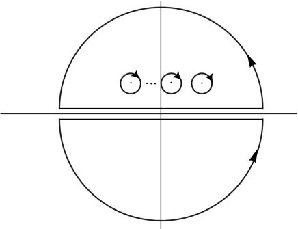
Figure 1: The integration path in (3.55).

We note that the integral over the two arc of the great semicircle tends to $0$ since (3.54). The right end of the above equation reduces to the sum of the residues

$$R(x,\lambda)=\frac{1}{2\pi i}\oint_{r_{j}}\frac{\Theta(x,\lambda^{{}^{\prime}})e^{-i\lambda^{{}^{\prime}}x-\int_{-\infty}^{x}udx}-\left(\begin{array}[]{c}1\\ 0\end{array}\right)}{\lambda^{{}^{\prime}}-\lambda}d\lambda^{{}^{\prime}}$$ (3.56)

at $\lambda_{j}$, and the continuous spectral component $J(x,\lambda)$

$$J(x,\lambda)=\frac{1}{2\pi i}\int_{-\infty}^{+\infty}\frac{r(\lambda^{{}^{\prime}})\psi(x,\lambda^{{}^{\prime}})e^{-i\lambda^{{}^{\prime}}x-\int_{-\infty}^{x}udx}}{\lambda^{{}^{\prime}}-\lambda}d\lambda^{{}^{\prime}}.$$ (3.57)

Applying (3.47), one obtains

$$R(x,\lambda)=\sum_{j=1}^{N}\frac{i}{\lambda-\lambda_{j}}c_{j}\psi(x,\lambda_{j})e^{-i\lambda_{j}x-\int_{-\infty}^{x}udx},$$ (3.58)

where $c_{j}=\frac{b_{j}}{a^{{}^{\prime}}(\lambda_{j})}$.
For the reflectionless case, when $Im(\lambda)<0$, have

$$\left(\begin{array}[]{c}\widetilde{\psi}_{1}(x,\lambda)\\ \widetilde{\psi}_{2}(x,\lambda)\end{array}\right)\cdot e^{-i\lambda x-\int_{-\infty}^{x}udx}-\left(\begin{array}[]{c}1\\ 0\end{array}\right)=\sum_{j=1}^{N}\frac{i}{\lambda-\lambda_{j}}c_{j}\left(\begin{array}[]{c}\psi_{1}(x,\lambda_{j})\\ \psi_{2}(x,\lambda_{j})\end{array}\right)e^{-i\lambda_{j}x-\int_{-\infty}^{x}udx}.$$ (3.59)

In addition, from (3.21), we have
$~{}~{}~{}~{}~{}~{}~{}~{}~{}~{}~{}~{}~{}~{}~{}~{}~{}~{}~{}~{}~{}~{}~{}~{}~{}~{}~{}~{}~{}~{}~{}~{}~{}~{}~{}~{}~{}~{}~{}~{}~{}~{}~{}~{}~{}~{}~{}~{}~{}~{}\psi(\lambda)-(-\widetilde{a}(\lambda)^{-1}\widetilde{\phi}(\lambda))=\widetilde{r}(\lambda)\widetilde{\psi}(\lambda)$,
where $\widetilde{r}(\lambda)=\frac{\widetilde{b}(\lambda)}{\widetilde{a}(\lambda)}$.

Define

$$\widetilde{\Theta}(x,\lambda)=\begin{cases}\phi(x,\lambda),~{}~{}~{}~{}~{}~{}~{}~{}~{}~{}~{}~{}~{}~{}Im\lambda>0,\\ -\widetilde{a}(\lambda)^{-1}\widetilde{\psi}(x,\lambda),~{}~{}~{}Im\lambda<0.\end{cases}$$ (3.60)

From (3.23), we know that

$$\widetilde{a}(\lambda) =\widetilde{\phi}_{1}(x,\lambda)\widetilde{\psi}_{2}(x,\lambda)-\widetilde{\psi}_{1}(x,\lambda)\widetilde{\phi}_{2}(x,\lambda)$$ (3.61)

$$=\left(\frac{v^{2}}{4\lambda^{2}}-1\right)\widetilde{\psi}_{1}(x,\lambda)\widetilde{\phi}_{2}(x,\lambda)$$

$$=-e^{\int_{-\infty}^{+\infty}\left(u-\frac{iv^{2}}{2\lambda}\right)dx}+o\left(\frac{1}{\lambda^{2}}\right).$$

Furthermore, we have

$$\begin{cases}\psi_{1}(x,\lambda)e^{i\lambda x+\int_{-\infty}^{x}udx}=o\left(\frac{1}{\lambda}\right),\\ \psi_{2}(x,\lambda)e^{i\lambda x+\int_{-\infty}^{x}udx}-1=o\left(\frac{1}{\lambda}\right),\\ \frac{\widetilde{\phi}_{2}(x,\lambda)}{-\widetilde{a}(\lambda)}e^{i\lambda x+\int_{-\infty}^{x}udx}-1=o\left(\frac{1}{\lambda}\right),\\ \frac{\widetilde{\phi}_{1}(x,\lambda)}{-\widetilde{a}(\lambda)}e^{i\lambda x+\int_{-\infty}^{x}udx}=o\left(\frac{1}{\lambda}\right),\end{cases}$$ (3.62)

which in turn yields

$$\widetilde{\Theta}(x,\lambda)e^{i\lambda x+\int_{-\infty}^{x}udx}-\left(\begin{array}[]{c}0\\ 1\end{array}\right)=o\left(\frac{1}{\lambda}\right).$$ (3.63)

According to Cauchy’s formula, we get

$$\widetilde{\Theta}(x,\lambda)\cdot e^{i\lambda x+\int_{-\infty}^{x}udx}-\left(\begin{array}[]{c}0\\ 1\end{array}\right)=\frac{1}{2\pi i}\oint\frac{\widetilde{\Theta}(x,\lambda^{{}^{\prime}})e^{i\lambda^{{}^{\prime}}x+\int_{-\infty}^{x}udx}-\left(\begin{array}[]{c}0\\ 1\end{array}\right)}{\lambda^{{}^{\prime}}-\lambda}d\lambda^{{}^{\prime}}.$$ (3.64)

where the integration path is shown in Fig. 2 and consists of two counterclockwise semicircles with radius tending to infinity and $N$ small clockwise circles $\widetilde{r}_{j},j=1,2,...N.$ containing the poles $\widetilde{\lambda}_{j},j=1,2,...N.$ of $\widetilde{\Theta}(x,\lambda)$.

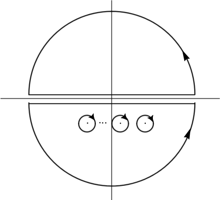
Figure 2: The integration path in (3.64).

We note that the integral over the two arc of the great semicircle tends to $0$ since (3.63). The right end of the above equation reduces to the sum of the residues

$$\widetilde{R}(x,\lambda)=\frac{1}{2\pi i}\oint_{\widetilde{r}_{j}}\frac{\widetilde{\Theta}(x,\lambda^{{}^{\prime}})e^{i\lambda^{{}^{\prime}}x+\int_{-\infty}^{x}udx}-\left(\begin{array}[]{c}1\\ 0\end{array}\right)}{\lambda^{{}^{\prime}}-\lambda}d\lambda^{{}^{\prime}}$$ (3.65)

at $\lambda_{j}$, and the continuous spectral component $J(x,\lambda)$

$$\widetilde{J}(x,\lambda)=\frac{1}{2\pi i}\int_{-\infty}^{+\infty}\frac{\widetilde{r}(\lambda^{{}^{\prime}})\widetilde{\psi}(x,\lambda^{{}^{\prime}})e^{i\lambda^{{}^{\prime}}x+\int_{-\infty}^{x}udx}}{\lambda^{{}^{\prime}}-\lambda}d\lambda^{{}^{\prime}}.$$ (3.66)

Through (3.48), we obtain

$$\widetilde{R}(x,\lambda)=\sum_{j=1}^{N}\frac{i}{\lambda-\widetilde{\lambda}_{j}}\tilde{c}_{j}\widetilde{\psi}(x,\widetilde{\lambda}_{j})e^{i\widetilde{\lambda}_{j}x-\int_{-\infty}^{x}udx},$$ (3.67)

where $\widetilde{c}_{j}=-\frac{\widetilde{b}_{j}}{\widetilde{a}^{{}^{\prime}}(\widetilde{\lambda}_{j})}$.
For the reflectionless case, when $Im(\lambda)>0$,

$$\left(\begin{array}[]{c}\psi_{1}(x,\lambda)\\ \psi_{2}(x,\lambda)\end{array}\right)e^{i\lambda x+\int_{-\infty}^{x}udx}-\left(\begin{array}[]{c}0\\ 1\end{array}\right)=\sum_{j=1}^{N}\frac{i}{\lambda-\widetilde{\lambda}_{j}}\tilde{c}_{j}\left(\begin{array}[]{c}\widetilde{\psi}_{1}(x,\widetilde{\lambda}_{j})\\ \widetilde{\psi}_{2}(x,\widetilde{\lambda}_{j})\end{array}\right)e^{i\widetilde{\lambda}_{j}x+\int_{-\infty}^{x}udx}.$$ (3.68)

3.3. The time dependence of the scattering data

In this subsection, we determine the time evolution of the non-isospectral scattering data.

From (2.1) and (3.23) we know that $a(\lambda)=\phi_{1}(x,\lambda)\psi_{2}(x,\lambda)-\psi_{1}(x,\lambda)\phi_{2}(x,\lambda)$, also have

$$a_{\lambda}(\lambda_{j}) =\left(\psi_{2,\lambda}(x,\lambda_{j})\phi_{1}(x,\lambda_{j})+\psi_{2}(x,\lambda_{j})\phi_{1,\lambda}(x,\lambda_{j})\right)-\left(\psi_{1,\lambda}(x,\lambda_{j})\phi_{2}(x,\lambda_{j})+\psi_{1}(x,\lambda_{j})\phi_{2,\lambda}(x,\lambda_{j})\right)$$ (3.69)

$$=\int_{-\infty}^{x}\frac{\partial}{\partial x}\left(\psi_{1,\lambda}(x,\lambda_{j})\phi_{2}(x,\lambda_{j})+\psi_{1}(x,\lambda_{j})\phi_{2,\lambda}(x,\lambda_{j})\right)dx$$

$$~{}~{}~{}-\int_{x}^{+\infty}\frac{\partial}{\partial x}\left(\psi_{2,\lambda}(x,\lambda_{j})\phi_{1}(x,\lambda_{j})+\psi_{2}(x,\lambda_{j})\phi_{1,\lambda}(x,\lambda_{j})\right)dx$$

$$=\int_{-\infty}^{+\infty}2ib_{j}\psi_{1}(x,\lambda_{j})\psi_{2}(x,\lambda_{j}).$$

Using $\sqrt{ic_{j}}\psi_{1}(x,\lambda_{j})$ instead of $\psi_{1}(x,\lambda_{j})$, $\sqrt{ic_{j}}\psi_{2}(x,\lambda_{j})$ instead of $\psi_{2}(x,\lambda_{j})$, we get

$$\int_{-\infty}^{+\infty}2\psi_{1}(x,\lambda_{j})\psi_{2}(x,\lambda_{j})=1.$$ (3.70)

$\mathbf{Lemma~{}3.4.}$ Suppose that $\psi(x,t,\lambda)$ is a solution of spectral problem (2.1), $M$ and $N$ satisfy the zero curvature equation (2.3), then

$$P(x,t,\lambda)=\psi_{t}(x,t,\lambda)-N\psi(x,t,\lambda)$$ (3.71)

is a solution of spectral problem (2.1) as well.
$\mathbf{Proof}$. By direct calculation, we get
$~{}~{}~{}~{}~{}~{}~{}~{}~{}~{}~{}~{}~{}~{}~{}~{}~{}~{}~{}~{}~{}~{}~{}~{}~{}~{}~{}~{}~{}~{}~{}~{}~{}~{}~{}~{}~{}~{}~{}~{}~{}P_{x}(x,t,\lambda)=\psi_{tx}(x,t,\lambda)-N_{x}\psi(x,t,\lambda)-N\psi_{x}(x,t,\lambda)$
$~{}~{}~{}~{}~{}~{}~{}~{}~{}~{}~{}~{}~{}~{}~{}~{}~{}~{}~{}~{}~{}~{}~{}~{}~{}~{}~{}~{}~{}~{}~{}~{}~{}~{}~{}~{}~{}~{}~{}~{}~{}~{}~{}~{}~{}~{}~{}~{}~{}~{}~{}~{}~{}~{}=(M\psi(x,t,\lambda))_{t}-N_{x}\psi(x,t,\lambda)-N\psi_{x}(x,t,\lambda)$
$~{}~{}~{}~{}~{}~{}~{}~{}~{}~{}~{}~{}~{}~{}~{}~{}~{}~{}~{}~{}~{}~{}~{}~{}~{}~{}~{}~{}~{}~{}~{}~{}~{}~{}~{}~{}~{}~{}~{}~{}~{}~{}~{}~{}~{}~{}~{}~{}~{}~{}~{}~{}~{}~{}=M_{t}\psi(x,t,\lambda)+M\psi_{t}(x,t,\lambda)-N_{x}\psi(x,t,\lambda)-N\psi_{x}(x,t,\lambda)$
$~{}~{}~{}~{}~{}~{}~{}~{}~{}~{}~{}~{}~{}~{}~{}~{}~{}~{}~{}~{}~{}~{}~{}~{}~{}~{}~{}~{}~{}~{}~{}~{}~{}~{}~{}~{}~{}~{}~{}~{}~{}~{}~{}~{}~{}~{}~{}~{}~{}~{}~{}~{}~{}~{}=MP(x,t,\lambda)$.
Therefore, $P(x,t,\lambda)$ is a solution of spectral problem (2.1).                                           $\Box$
$\mathbf{Definition~{}3.1.}$ For brevity, we define the vector operations $\cdot$ and $\langle,\rangle$ as
$~{}~{}~{}~{}~{}~{}~{}~{}~{}~{}~{}~{}~{}~{}~{}~{}~{}~{}~{}~{}~{}~{}~{}~{}~{}~{}~{}~{}~{}~{}~{}~{}~{}~{}~{}~{}~{}~{}\left(\begin{array}[]{c}z_{1}\\ z_{2}\end{array}\right)\cdot\left(\begin{array}[]{c}y_{1}\\ y_{2}\end{array}\right)=z_{1}y_{1}+z_{2}y_{2}$,
$~{}~{}~{}~{}~{}~{}~{}~{}~{}~{}~{}~{}~{}~{}~{}~{}~{}~{}~{}~{}~{}~{}~{}~{}~{}~{}~{}~{}~{}~{}~{}~{}~{}~{}~{}~{}~{}~{}\left\langle\left(\begin{array}[]{c}z_{1}\\ z_{2}\end{array}\right),\left(\begin{array}[]{c}y_{1}\\ y_{2}\end{array}\right)\right\rangle=\int_{-\infty}^{+\infty}\left(z_{1}y_{1}+z_{2}y_{2}\right)dx$.
$\mathbf{Theorem~{}3.1.}$ The discrete scattering data ${\lambda_{j}(t),c_{j}(t)}$ for $\psi(x,t,\lambda)$ and $\phi(x,t,\lambda)$ have the following time dependence. For $n=0$,

$$\begin{cases}\lambda_{j}(t)=e^{t+\ln\lambda_{j}},\\ c_{j}(t)=e^{t+\ln c_{j}(t)},\end{cases}$$ (3.72)

For $n\geq 1$,

$$\begin{cases}\lambda_{j}(t)=\left(\lambda_{j}(0)^{-n}-nt\right)^{-\frac{1}{n}},\\ c_{j}(t)=\frac{c_{j}(0)}{\lambda_{j}(0)^{n+1}}\left(\lambda_{j}(0)^{-n}-nt\right)^{-\frac{n+1}{n}},\end{cases}$$ (3.73)

where $\lambda_{j}(0)$ and $c_{j}(0)$ are the scattering data of spectral problem (2.1) in terms of $u(0,x)$ and $v(0,x)$.
$\mathbf{Proof}$. Taking $\lambda=\lambda_{j}$ (where $Im\lambda_{j}>0)$ and replacing the normalization eigenfunction $\sqrt{ic_{j}}\psi(x,\lambda_{j})$ of spectral problem (2.1) by $\psi(x,\lambda_{j})$, and based on Lemma 3.4, we know
$~{}~{}~{}~{}~{}~{}~{}~{}~{}~{}~{}~{}~{}~{}~{}~{}~{}~{}~{}~{}~{}~{}~{}~{}~{}~{}~{}~{}~{}~{}~{}~{}~{}~{}~{}~{}~{}~{}~{}~{}~{}~{}~{}~{}~{}~{}~{}~{}~{}~{}~{}~{}P(x,\lambda_{j})=\psi_{t}(x,\lambda_{j})-N\psi(x,\lambda_{j})$
is still a solution of spectral problem (2.1). There exist two constants $\beta$ and $\theta$, such that

$$\psi_{t}(x,\lambda_{j})-N\psi(x,\lambda_{j})=\beta\psi(x,\lambda_{j})+\theta\widetilde{\psi}(x,\lambda_{j}).$$ (3.74)

We can find $\theta=0$ because $\psi_{1}(x,\lambda_{j})$ tends to zero while $\widetilde{\psi}_{1}(x,\lambda_{j})$ tends to infinite when $x\rightarrow+\infty$. So (3.74) reads

$$\psi_{t}(x,\lambda_{j})-N\psi(x,\lambda_{j})=\beta\psi(x,\lambda_{j}).$$ (3.75)

To derive the value of $\beta$, multiplying (3.75) by $\left(\psi_{2}(x,\lambda_{j}),\psi_{1}(x,\lambda_{j})\right)^{T}$ ($T$ is the transpose of the matrix), we get

$$\int_{-\infty}^{+\infty}[2(\psi_{1}(x,\lambda_{j})\psi_{2}(x,\lambda_{j}))_{t}-A\psi_{1}(x,\lambda_{j})\psi_{2}(x,\lambda_{j})-(B+C)\psi_{2}^{2}(x,\lambda_{j})$$ (3.76)

$$-(B-C)\psi_{1}^{2}(x,\lambda_{j})+A\psi_{2}(x,\lambda_{j})\psi_{1}(x,\lambda_{j})]dx=\beta.$$

Through (3.70), we obtain

$$\int_{-\infty}^{+\infty}\left(-(B+C)\psi_{2}^{2}(x,\lambda_{j})-(B-C)\psi_{1}^{2}(x,\lambda_{j})\right)dx=\beta.$$ (3.77)

Calculating (3.77) yield

$$\beta =-\int_{-\infty}^{+\infty}\left(\begin{array}[]{l}B+C\\ B-C\end{array}\right)\left(\begin{array}[]{l}\psi_{2}^{2}(x,\lambda_{j})\\ \psi_{1}^{2}(x,\lambda_{j})\end{array}\right)dx$$ (3.78)

$$=-\int_{-\infty}^{+\infty}\sum_{i=0}^{n}\left(\begin{array}[]{c}b_{i+1}+c_{i}\\ b_{i+1}-c_{i}\end{array}\right)\left(\begin{array}[]{l}\psi_{2}^{2}(x,\lambda_{j})\\ \psi_{1}^{2}(x,\lambda_{j})\end{array}\right)dx\cdot\lambda_{j}^{n-i}$$

$$=-(n+1)\int_{-\infty}^{+\infty}b_{1}\left(\psi_{2}^{2}(x,\lambda_{j})+\psi_{1}^{2}(x,\lambda_{j})\right)\lambda_{j}^{n}dx$$

$$=-(n+1)\int_{-\infty}^{+\infty}vx\left(\psi_{1}^{2}(x,\lambda_{j})+\psi_{2}^{2}(x,\lambda_{j})\right)\lambda_{j}^{n}dx$$

$$=(n+1)\int_{-\infty}^{+\infty}\psi_{1}(x,\lambda_{j})\psi_{2}(x,\lambda_{j})dx\lambda_{j}^{n}$$

$$=\frac{\lambda_{j}^{n}}{2}\cdot(n+1).$$

From (3.3) and (3.75), we get

$$\psi_{t}(x,\lambda_{j})-N\psi(x,\lambda_{j})$$ (3.79)

$$= -ix\lambda_{j,t}\left(\begin{array}[]{cc}0\\ 1\end{array}\right)e^{-i\lambda_{j}x}\sqrt{ic_{j}}+(\sqrt{ic_{j}})_{t}\left(\begin{array}[]{l}0\\ 1\end{array}\right)e^{-i\lambda_{j}x}$$

$$-\left(\begin{array}[]{cc}ix\lambda_{j}^{n+1}&0\\ 0&-ix\lambda_{j}^{n+1}\end{array}\right)\left(\begin{array}[]{l}0\\ 1\end{array}\right)e^{-i\lambda_{j}x}\sqrt{ic_{j}}$$

$$= \frac{n+1}{2}\lambda_{j}^{n}\left(\begin{array}[]{l}0\\ 1\end{array}\right)e^{-i\lambda_{j}x}\sqrt{ic_{j}}.$$

as $x\rightarrow-\infty$. It can be deduced that
$~{}~{}~{}~{}~{}~{}~{}~{}~{}~{}~{}~{}~{}~{}~{}~{}~{}~{}~{}~{}-ix\lambda_{j,t}\left(\begin{array}[]{l}0\\ 1\end{array}\right)e^{-i\lambda_{j}x}\sqrt{ic_{j}}=-\left(\begin{array}[]{cc}ix\lambda_{j}^{n+1}&0\\ 0&-ix\lambda_{j}^{n+1}\end{array}\right)\left(\begin{array}[]{l}0\\ 1\end{array}\right)e^{-i\lambda_{j}x}\sqrt{ic_{j}}$
and
$~{}~{}~{}~{}~{}~{}~{}~{}~{}~{}~{}~{}~{}~{}~{}~{}~{}~{}~{}~{}~{}~{}~{}~{}~{}~{}~{}~{}~{}~{}~{}~{}~{}~{}~{}~{}~{}~{}~{}~{}~{}~{}~{}~{}~{}~{}~{}~{}~{}~{}~{}~{}~{}~{}~{}~{}~{}~{}~{}(\sqrt{ic_{j}})_{t}=\frac{n+1}{2}\lambda^{n}\sqrt{ic_{j}}$.
Thus we have
$~{}~{}~{}~{}~{}~{}~{}~{}~{}~{}~{}~{}~{}~{}~{}~{}~{}~{}~{}~{}~{}~{}~{}~{}~{}~{}~{}~{}~{}~{}~{}~{}~{}~{}~{}~{}~{}~{}~{}~{}~{}~{}~{}~{}~{}~{}~{}~{}~{}~{}~{}~{}~{}~{}~{}~{}~{}~{}~{}~{}~{}~{}c_{j,t}=(n+1)\lambda_{j}^{n}c_{j}$.
Since $\lambda_{t}=\lambda^{n+1}$, we can prove the theorem directly.                                                                          $\Box$

On the other hand, from (3.23), we derive that
$~{}~{}~{}~{}~{}~{}~{}~{}~{}~{}~{}~{}~{}~{}~{}~{}~{}~{}~{}~{}~{}~{}~{}~{}~{}~{}~{}~{}~{}~{}~{}~{}~{}~{}~{}~{}~{}~{}~{}~{}~{}~{}~{}~{}~{}~{}~{}~{}~{}~{}~{}~{}~{}~{}~{}~{}~{}~{}~{}~{}~{}\widetilde{a}(\lambda)=\widetilde{\phi}_{1}(x,\lambda)\widetilde{\psi}_{2}(x,\lambda)-\widetilde{\psi}_{1}(x,\lambda)\widetilde{\phi}_{2}(x,\lambda)$.
In this case,

$$\widetilde{a}_{\lambda}(\lambda) =\left(\widetilde{\phi}_{1,\lambda}(x,\lambda)\widetilde{\psi}_{2}(x,\lambda)+\widetilde{\phi}_{1}(x,\lambda)\widetilde{\psi}_{2,\lambda}(x,\lambda)\right)-\left(\widetilde{\psi}_{1,\lambda}(x,\lambda)\widetilde{\phi}_{2}(x,\lambda)+\widetilde{\psi}_{1}(x,\lambda)\widetilde{\phi}_{2,\lambda}(x,\lambda)\right)$$ (3.80)

$$=\int_{-\infty}^{x}\frac{\partial}{\partial x}\left(\widetilde{\phi}_{1,\lambda}(x,\lambda)\widetilde{\psi}_{2}(x,\lambda)-\widetilde{\psi}_{1}(x,\lambda)\widetilde{\phi}_{2,\lambda}(x,\lambda)\right)dx-\int_{x}^{+\infty}\frac{\partial}{\partial x}\left(\widetilde{\phi}_{1}(x,\lambda)\widetilde{\psi}_{2,\lambda}(x,\lambda)-\widetilde{\psi}_{1,\lambda}(x,\lambda)\widetilde{\phi}_{2}(x,\lambda)\right)dx.$$

When $\lambda=\widetilde{\lambda}_{j}$, we note that $\widetilde{\phi}_{1}(x,\widetilde{\lambda}_{j})=\widetilde{b}_{j}\widetilde{\psi}_{1}(x,\widetilde{\lambda}_{j})$. Thus

$$\widetilde{a}_{\lambda}(\widetilde{\lambda}_{j})=\int_{-\infty}^{+\infty}2i\widetilde{b}_{j}\widetilde{\psi}_{1}(x,\widetilde{\lambda}_{j})\widetilde{\psi}_{2}(x,\widetilde{\lambda}_{j})dx,$$ (3.81)

that is

$$\int_{-\infty}^{+\infty}-2i\widetilde{c}_{j}\widetilde{\psi}_{1}(x,\widetilde{\lambda}_{j})\widetilde{\psi}_{2}(x,\widetilde{\lambda}_{j})dx=1,$$ (3.82)

where we define that $\widetilde{c}_{j}=-\frac{\widetilde{b}_{j}}{\widetilde{a}^{{}^{\prime}}(\widetilde{\lambda}_{j})}$.
$\mathbf{Lemma~{}3.5.}$ Suppose that $\widetilde{\psi}\left(x,t,\lambda\right)$ is a solution of spectral problem (2.1), $M$ and $N$ satisfy the zero curvature equation (2.3), then

$$P\left(x,t,\lambda\right)=\widetilde{\psi}_{t}\left(x,t,\lambda\right)-N\widetilde{\psi}\left(x,t,\lambda\right)$$ (3.83)

is a solution of spectral problem (2.1) as well.
$\mathbf{Theorem~{}3.2}$ The discrete scattering data ${\widetilde{\lambda}_{j}(t),\widetilde{c}_{j}(t)}$ for $\widetilde{\psi}(x,t,\lambda)$ and $\widetilde{\phi}(x,t,\lambda)$ posses the following time dependence. For $n=0$,

$$\begin{cases}\widetilde{\lambda}_{j}(t)=e^{t+\ln\widetilde{\lambda}_{j}},\\ \widetilde{c}_{j}(t)=e^{t+\ln\widetilde{c}_{j}(t)},\end{cases}$$ (3.84)

For $n\geq 1$,

$$\begin{cases}\widetilde{\lambda}_{j}(t)=\left(\widetilde{\lambda}_{j}(0)^{-n}-nt\right)^{-\frac{1}{n}},\\ \widetilde{c}_{j}(t)=\frac{\widetilde{c}_{j}(0)}{\widetilde{\lambda}_{j}(0)^{n+1}}\left(\widetilde{\lambda}_{j}(0)^{-n}-nt\right)^{-\frac{n+1}{n}},\end{cases}$$ (3.85)

where $\widetilde{\lambda}_{j}(0)$ and $\widetilde{c}_{j}(0)$ are the scattering data of spectral problem (2.1) in terms of $u(0,x)$ and $v(0,x)$.
$\mathbf{Proof}$. Based on Lemma 3.5, we have

$$\widetilde{\psi}_{t}(x,\widetilde{\lambda}_{j})-N\widetilde{\psi}(x,\widetilde{\lambda}_{j})=\gamma\widetilde{\psi}(x,\widetilde{\lambda}_{j}),$$ (3.86)

where $\gamma$ is a constant to be determined here. Similar with (3.76), we have

$$\int_{-\infty}^{+\infty}\left(-(B+C)\widetilde{\psi}_{2}^{2}(x,\widetilde{\lambda}_{j})-(B-C)\widetilde{\psi}_{1}^{2}(x,\widetilde{\lambda}_{j})\right)dx=\gamma.$$ (3.87)

Therefore,

$$\gamma =-\int_{-\infty}^{+\infty}\left(\begin{array}[]{c}B+C\\ B-C\end{array}\right)\left(\begin{array}[]{cc}\widetilde{\psi}_{2}(x,\widetilde{\lambda}_{j})\\ \widetilde{\psi}_{1}(x,\widetilde{\lambda}_{j})\end{array}\right)$$ (3.88)

$$=-\sum_{k=0}^{n}\int_{-\infty}^{+\infty}\widetilde{\lambda}_{j}^{k}\left(\begin{array}[]{cc}b_{1}+c_{0}\\ b_{1}-c_{0}\end{array}\right)\left(\begin{array}[]{c}\widetilde{\psi}_{2}^{2}(x,\widetilde{\lambda}_{j})\\ \widetilde{\psi}_{1}^{2}(x,\widetilde{\lambda}_{j})\end{array}\right)\widetilde{\lambda}_{j}^{n-k}dx$$

$$=\frac{n+1}{2}\widetilde{\lambda}_{j}^{n}.$$

Through (3.3), it is noted that
$~{}~{}~{}~{}~{}~{}~{}~{}~{}~{}~{}~{}~{}~{}~{}~{}~{}~{}~{}~{}~{}~{}~{}~{}~{}~{}~{}~{}~{}~{}~{}~{}~{}~{}~{}~{}~{}~{}~{}~{}~{}~{}~{}~{}~{}\widetilde{\psi}(x,\widetilde{\lambda}_{j})\sim\left(\begin{array}[]{c}1\\ 0\end{array}\right)e^{i\widetilde{\lambda}_{j}x}\sqrt{-i\widetilde{c}_{j}}$ as $x\rightarrow-\infty$,
which indicate that

$$\widetilde{\psi}_{t}(x,\widetilde{\lambda}_{j})-N\widetilde{\psi}(x,\widetilde{\lambda}_{j})$$ (3.89)

$$= i\widetilde{\lambda}_{j,t}x\left(\begin{array}[]{c}1\\ 0\end{array}\right)e^{i\widetilde{\lambda}_{j}x}\sqrt{-i\widetilde{c}_{j}}+\left(\begin{array}[]{c}1\\ 0\end{array}\right)e^{i\widetilde{\lambda}_{j}x}\left(\sqrt{-i\tilde{c}_{j}}\right)_{t}$$

$$-\left(\begin{array}[]{cc}ix\widetilde{\lambda}_{j}^{n+1}&0\\ 0&-ix\widetilde{\lambda}_{j}^{n+1}\end{array}\right)\left(\begin{array}[]{c}1\\ 0\end{array}\right)e^{i\widetilde{\lambda}_{j}x}\sqrt{-i\tilde{c}_{j}}$$

$$= \frac{n+1}{2}\widetilde{\lambda}_{j}^{n}\left(\begin{array}[]{c}1\\ 0\end{array}\right)e^{i\widetilde{\lambda}_{j}x}\sqrt{-i\widetilde{c}_{j}}.$$

Thus we obtain
$~{}~{}~{}~{}~{}~{}~{}~{}~{}~{}~{}~{}~{}~{}~{}~{}~{}~{}~{}~{}~{}~{}~{}~{}~{}~{}~{}~{}~{}~{}~{}~{}~{}~{}~{}~{}~{}~{}~{}~{}~{}~{}~{}~{}~{}~{}~{}~{}~{}~{}\left(\sqrt{-i\tilde{c}_{j}}\right)_{t}=\frac{n+1}{2}\widetilde{\lambda}_{j}^{n}\sqrt{-i\tilde{c}_{j}}$
and
$~{}~{}~{}~{}~{}~{}~{}~{}~{}~{}~{}~{}~{}~{}~{}~{}~{}~{}~{}~{}~{}~{}~{}~{}~{}~{}~{}~{}~{}~{}~{}~{}~{}~{}~{}~{}~{}~{}~{}~{}~{}~{}~{}~{}~{}~{}~{}~{}~{}~{}~{}~{}~{}~{}\tilde{c}_{j,t}=(n+1)\widetilde{\lambda}_{j}^{n}\tilde{c}_{j}.$

$\Box$

3.4. General solutions for the non-isospectral TD hierarchy

From (3.59) and (3.68) respectively,

$$\widetilde{\psi}(x,\widetilde{\lambda}_{k})=\left(\begin{array}[]{c}1\\ 0\end{array}\right)e^{i\widetilde{\lambda}_{k}x+\int_{-\infty}^{x}udx}+\sum_{j=1}^{N}\frac{i}{\widetilde{\lambda}_{k}-\lambda_{j}}c_{j}\psi(x,\lambda_{j})e^{i(\widetilde{\lambda}_{k}-\lambda_{j})x},$$ (3.90)

and

$$\psi(x,\lambda_{k})=\left(\begin{array}[]{c}0\\ 1\end{array}\right)e^{-i\lambda_{k}x-\int_{-\infty}^{x}udx}+\sum_{j=1}^{N}\frac{i}{\lambda_{k}-\widetilde{\lambda}_{j}}\widetilde{c}_{j}\widetilde{\psi}(x,\widetilde{\lambda}_{j})e^{i(\widetilde{\lambda}_{j}-\lambda_{k})x}.$$ (3.91)

Thus we have

$$\widetilde{\psi}_{1}(x,\widetilde{\lambda}_{k})e^{-i\widetilde{\lambda}_{k}x-\int_{-\infty}^{x}udx}=1+\sum_{j=1}^{N}\frac{i}{\widetilde{\lambda}_{k}-\lambda_{j}}c_{j}\psi_{1}(x,\lambda_{j})e^{-i\widetilde{\lambda}_{j}x-\int_{-\infty}^{x}udx},$$ (3.92)

and

$$\psi_{1}(x,\lambda_{k})e^{i\lambda_{k}x+\int_{-\infty}^{x}udx}=\sum_{j=1}^{N}\frac{i}{\lambda_{k}-\widetilde{\lambda}_{j}}\widetilde{c}_{j}\widetilde{\psi}_{1}(x,\widetilde{\lambda}_{j})e^{i\widetilde{\lambda}_{j}x+\int_{-\infty}^{x}udx}.$$ (3.93)

By (3.92) and (3.93), we get

$$~{}~{}~{}\psi_{1}(x,\lambda_{k})e^{-i\lambda_{k}x-\int_{-\infty}^{x}udx}$$ (3.94)

$$=\sum_{j=1}^{N}\frac{i}{\lambda_{k}-\widetilde{\lambda}_{j}}\widetilde{c}_{j}\widetilde{\psi}_{1}(x,\widetilde{\lambda}_{j})e^{i(\widetilde{\lambda}_{j}-2\lambda_{k})x-\int_{-\infty}^{x}udx}$$

$$=\sum_{j=1}^{N}\frac{i}{\lambda_{k}-\widetilde{\lambda}_{j}}\widetilde{c}_{j}\widetilde{\psi}_{1}(x,\widetilde{\lambda}_{j})e^{-i\widetilde{\lambda}_{j}x-\int_{-\infty}^{x}udx}\cdot e^{2i(\widetilde{\lambda}_{j}-\lambda_{k})x}$$

$$=\sum_{j=1}^{N}\frac{i}{\lambda_{k}-\widetilde{\lambda}_{j}}\widetilde{c}_{j}e^{2i(\widetilde{\lambda}_{j}-\lambda_{k})x}\cdot\left(1+\sum_{k=1}^{N}\frac{i}{\widetilde{\lambda}_{j}-\lambda_{k}}c_{k}\psi_{1}(x,\lambda_{k})e^{-i\widetilde{\lambda}_{k}x-\int_{-\infty}^{x}udx}\right),$$

Then we multiply the left and right sides of (3.94) by $c_{k}$, and get

$$~{}~{}~{}c_{k}\psi_{1}(x,\lambda_{k})e^{-i\lambda_{k}x-\int_{-\infty}^{x}udx}-c_{k}\sum_{j=1}^{N}\frac{i}{\lambda_{k}-\widetilde{\lambda}_{j}}\widetilde{c}_{j}\cdot\left(\sum_{k=1}^{N}\frac{i}{\widetilde{\lambda}_{j}-\lambda_{k}}c_{k}\psi_{1}(x,\lambda_{k})e^{-i\widetilde{\lambda}_{k}x-\int_{-\infty}^{x}udx}\right)e^{2i(\widetilde{\lambda}_{j}-\lambda_{k})x}$$ (3.95)

$$=c_{k}\sum_{j=1}^{N}\frac{i}{\lambda_{k}-\widetilde{\lambda}_{j}}\widetilde{c}_{j}e^{2i(\widetilde{\lambda}_{j}-\lambda_{k})x}.$$

This is a solvable system of $N$-member linear equations with respect to $c_{k}\psi_{1}(x,\lambda_{k})e^{-i\lambda_{k}x-\int_{-\infty}^{x}udx}$.

$\mathbf{Theorem~{}3.3}$

$$\frac{iv^{2}}{2}=\sum_{j=1}^{N}ic_{j}\left(\psi_{1}(x,\lambda_{j})e^{-i\lambda_{j}x-\int_{-\infty}^{x}udx}\right)_{x}.$$ (3.96)

$\mathbf{Proof.}$ Since (3.19), we know $\widetilde{\psi}_{1}(x,\lambda)e^{-i\lambda x-\int_{-\infty}^{x}udx+o(\lambda^{-2})}$ has the following asymptotic property that

$$~{}~{}~{}\widetilde{\psi}_{1}(x,\lambda)e^{-i\lambda x-\int_{-\infty}^{x}udx+o(\lambda^{-2})}$$ (3.97)

$$=e^{\int_{-\infty}^{x}-\frac{iv^{2}}{2\lambda}dx+o(\lambda^{-2})},$$

$$=1+\frac{1}{2\lambda}\int_{-\infty}^{x}iv^{2}dx+o(\lambda^{-2})$$

as $\lambda\rightarrow\infty$.

Thus we can obtain an expression for $v$ by deriving both sides of (3.97) with respect to $x$,

$$\frac{iv^{2}}{2}=\lim_{\lambda\rightarrow\infty}\lambda\left(\widetilde{\psi}_{1}(x,\lambda)e^{-i\lambda x-\int_{-\infty}^{x}udx}-1\right)_{x}.$$ (3.98)

Substituting (3.59) into (3.98) to replace $\widetilde{\psi}_{1}(x,\lambda)e^{-i\lambda x-\int_{-\infty}^{x}udx}$ with $\psi_{1}(x,\lambda_{j})e^{-i\lambda_{j}x-\int_{-\infty}^{x}udx}$, we obtain

$$\frac{iv^{2}}{2}=\lim_{\lambda\rightarrow\infty}\sum_{j=1}^{N}\frac{i\lambda}{\lambda-\lambda_{j}}\left(c_{j}\psi_{1}(x,\lambda_{j})e^{-i\lambda_{j}x-\int_{-\infty}^{x}udx}\right)_{x}.$$ (3.99)

Thus the Theorem 3.3 is proved.                                                                           $\Box$

From the solvable system (LABEL:solution4) and Theorem 3.3, we can derive that

$$v=\pm\sqrt{2\left((D^{-1}F)^{T}\cdot\left(\begin{array}[]{c}1\\ \vdots\\ 1\end{array}\right)\right)_{x}~{}~{}},$$ (3.100)

where
$~{}~{}~{}~{}~{}~{}~{}~{}~{}~{}~{}~{}~{}~{}~{}~{}~{}~{}~{}~{}~{}~{}~{}~{}~{}~{}~{}~{}~{}~{}~{}~{}~{}~{}~{}~{}~{}~{}~{}~{}~{}~{}~{}~{}~{}~{}~{}~{}~{}~{}~{}~{}~{}~{}~{}~{}~{}~{}~{}~{}D=I+d_{N\times N}$
with
$~{}~{}~{}~{}~{}~{}~{}~{}~{}~{}~{}~{}~{}~{}~{}~{}~{}~{}~{}~{}~{}~{}~{}~{}~{}~{}~{}~{}~{}~{}~{}~{}~{}~{}~{}~{}~{}~{}~{}~{}~{}~{}~{}~{}~{}~{}~{}~{}~{}~{}~{}~{}d_{kj}=c_{k}\sum_{j=1}^{N}\frac{\widetilde{c}_{j}e^{2i(\widetilde{\lambda}_{j}-\lambda_{j})x}}{\left(\lambda_{k}-\widetilde{\lambda}_{j}\right)\left(\widetilde{\lambda}_{j}-\lambda_{k}\right)}$,
and
$~{}~{}~{}~{}~{}~{}~{}~{}~{}~{}~{}~{}~{}~{}~{}~{}~{}~{}~{}~{}~{}~{}~{}~{}~{}~{}~{}~{}~{}~{}~{}~{}~{}~{}~{}~{}~{}~{}~{}~{}~{}~{}~{}~{}~{}~{}~{}~{}~{}~{}~{}~{}~{}~{}~{}~{}~{}~{}~{}~{}F=\left(\begin{array}[]{c}\beta_{1}\\ \vdots\\ \beta_{N}\end{array}\right)$
with
$~{}~{}~{}~{}~{}~{}~{}~{}~{}~{}~{}~{}~{}~{}~{}~{}~{}~{}~{}~{}~{}~{}~{}~{}~{}~{}~{}~{}~{}~{}~{}~{}~{}~{}~{}~{}~{}~{}~{}~{}~{}~{}~{}~{}~{}~{}\beta_{k}=c_{k}\sum_{k=1}^{N}\frac{i}{\lambda_{k}-\widetilde{\lambda}_{k}}\widetilde{c}_{k}e^{2i(\widetilde{\lambda}_{k}-\lambda_{k})x}$.

By now we have obtained an explicit expression for the $N$-soliton solution of $v$. It is worth noting that the expression for $u$ can be obtained by substituting $v$ in the second equation of (2.12). In this case, the second equation of (2.12) is an ordinary differential equation with respect to $u$ as $v=$(3.100).

4. l-soliton-like solution

In this section, we follow the example of the previous section to obtain the explicit expression for the l-soliton-like solution of non-isospectral TD hierarchy as $N=1$.

Let $\lambda=\widetilde{\lambda}_{1}$ in (3.59), we note that

$$\widetilde{\psi}_{1}(x,\widetilde{\lambda}_{1})e^{-i\widetilde{\lambda}_{1}x-\int_{-\infty}^{x}udx}=1+\frac{i}{\widetilde{\lambda}_{1}-\lambda_{1}}c_{1}\psi_{1}(x,\lambda_{1})e^{-i\lambda_{1}x-\int_{-\infty}^{x}udx}.$$ (4.1)

Similarly in (3.68), let $\lambda=\lambda_{1}$,we get From (3.68), we get

$$e^{i\lambda_{1}x+\int_{-\infty}^{x}udx}\psi_{1}(x,\lambda_{1})=\frac{i}{\lambda_{1}-\widetilde{\lambda}_{1}}\widetilde{c}_{1}\widetilde{\psi}_{1}(x,\widetilde{\lambda}_{1})e^{i\widetilde{\lambda}_{1}x+\int_{-\infty}^{x}udx}.$$ (4.2)

Substituting (4.2) into (4.1) yields

$$\begin{cases}\widetilde{\psi}_{1}(x,\widetilde{\lambda}_{1})e^{-i\widetilde{\lambda}_{1}x-\int_{-\infty}^{x}udx}=1+\frac{i}{\widetilde{\lambda}_{1}-\lambda_{1}}c_{1}\widetilde{c}_{1}\frac{i}{\lambda_{1}-\widetilde{\lambda}_{1}}\widetilde{\psi}_{1}(x,\widetilde{\lambda}_{1})e^{i\widetilde{\lambda}_{1}x+\int_{-\infty}^{x}udx}e^{-2i\lambda_{1}x-2\int_{-\infty}^{x}udx},\\ \psi_{1}(x,\lambda_{1})e^{i\lambda_{1}x+\int_{-\infty}^{x}udx}=\frac{i}{\lambda_{1}-\widetilde{\lambda}_{1}}\widetilde{c}_{1}e^{2i\widetilde{\lambda}_{1}x+2\int_{-\infty}^{x}udx}\left(1+\frac{i}{\widetilde{\lambda}_{1}-\lambda_{1}}c_{1}\psi_{1}(x,\lambda_{1})e^{-i\lambda_{1}x-\int_{-\infty}^{x}udx}\right).\end{cases}$$ (4.3)

Let
$~{}~{}~{}~{}~{}~{}~{}~{}~{}~{}~{}~{}~{}~{}~{}~{}~{}~{}~{}~{}~{}~{}~{}~{}~{}~{}~{}~{}~{}~{}~{}~{}~{}~{}~{}~{}~{}~{}~{}~{}~{}~{}~{}~{}~{}~{}~{}~{}~{}~{}~{}~{}~{}~{}~{}~{}~{}T=\psi_{1}(x,\lambda_{j})e^{-i\lambda_{j}x-\int_{-\infty}^{x}udx}$,
we have
$~{}~{}~{}~{}~{}~{}~{}~{}~{}~{}~{}~{}~{}~{}~{}~{}~{}~{}~{}~{}~{}~{}~{}~{}~{}~{}~{}~{}~{}~{}~{}~{}~{}~{}~{}~{}~{}~{}~{}~{}~{}~{}~{}~{}~{}~{}~{}~{}~{}T=\frac{i}{\lambda_{1}-\widetilde{\lambda}_{1}}\widetilde{c}_{1}e^{2i(\widetilde{\lambda}_{1}-\lambda_{1})x}\left(1+\frac{i}{\widetilde{\lambda}_{1}-\lambda_{1}}c_{1}T\right)$.
So that

$$T =\frac{\frac{i}{\lambda_{1}-\widetilde{\lambda}_{1}}\widetilde{c}_{1}e^{2i(\widetilde{\lambda}_{1}-\lambda_{1})x}}{1-\frac{1}{(\lambda_{1}-\widetilde{\lambda}_{1})^{2}}c_{1}\widetilde{c}_{1}e^{2i(\widetilde{\lambda}_{1}-\lambda_{1})x}}$$ (4.4)

$$=\frac{i}{\lambda_{1}-\widetilde{\lambda}_{1}}\widetilde{c}_{1}\cdot\frac{1}{e^{2i(\lambda_{1}-\widetilde{\lambda}_{1})x}-\frac{1}{(\lambda_{1}-\widetilde{\lambda}_{1})^{2}}c_{1}\widetilde{c}_{1}}.$$

Therefore, we get

$$T_{x} =\frac{i}{\lambda_{1}-\widetilde{\lambda}_{1}}\tilde{c}_{1}\cdot\frac{-e^{2i\left(\lambda_{1}-\widetilde{\lambda}_{1}\right)x}\cdot 2i\left(\lambda_{1}-\widetilde{\lambda}_{1}\right)}{\left(e^{2i\left(\lambda_{1}-\widetilde{\lambda}_{1}\right)x}-\frac{1}{\left(\lambda_{1}-\widetilde{\lambda}_{1}\right)^{2}}c_{1}\widetilde{c}_{1}\right)^{2}}$$ (4.5)

$$=\frac{2\widetilde{c}_{1}e^{2i\left(\lambda_{1}-\widetilde{\lambda}_{1}\right)x}}{\left(e^{2i\left(\lambda_{1}-\widetilde{\lambda}_{1}\right)x}-\frac{1}{\left(\lambda_{1}-\widetilde{\lambda}_{1}\right)^{2}}c_{1}\widetilde{c}_{1}\right)^{2}}$$

$$=\frac{2\widetilde{c}_{1}}{\left(e^{i\left(\lambda_{1}-\widetilde{\lambda}_{1}\right)x}-\frac{1}{\left(\lambda_{1}-\widetilde{\lambda}_{1}\right)^{2}}c_{1}\widetilde{c_{1}}e^{i\left(\widetilde{\lambda}_{1}-\lambda_{1}\right)x}\right)^{2}}$$

$$=\frac{2\widetilde{c}_{1}\frac{\left(\lambda_{1}-\widetilde{\lambda}_{1}\right)^{2}}{c_{1}\widetilde{c}_{1}}}{\left(\frac{\lambda_{1}-\widetilde{\lambda}_{1}}{\sqrt{c_{1}\tilde{c}_{1}}}e^{i\left(\lambda_{1}-\widetilde{\lambda}_{1}\right)x}-\frac{\sqrt{c_{1}\widetilde{c}_{1}}}{\lambda_{1}-\widetilde{\lambda}_{1}}e^{i\left(\widetilde{\lambda}_{1}-\lambda_{1}\right)x}\right)^{2}}.$$

Since $cschx=\frac{2}{e^{x}-e^{-x}}$, then we can derive that

$$T_{x}=\frac{(\lambda_{1}-\widetilde{\lambda}_{1})^{2}csch^{2}\left(i(\lambda_{1}-\widetilde{\lambda}_{1})x+\ln\left(\frac{\lambda_{1}-\widetilde{\lambda}_{1}}{\sqrt{c_{1}\widetilde{c}_{1}}}\right)\right)}{c_{1}}.$$ (4.6)

Finally, we get the explicit expression for $v$ that

$$v^{2} =2c_{1}T_{x}$$ (4.7)

$$=2(\lambda_{1}-\widetilde{\lambda}_{1})^{2}csch^{2}\left(i(\lambda_{1}-\widetilde{\lambda}_{1})x+\ln\left(\frac{\lambda_{1}-\widetilde{\lambda}_{1}}{\sqrt{c_{1}\widetilde{c}_{1}}}\right)\right),$$

that is

$$v=\pm\sqrt{2}(\lambda_{1}-\widetilde{\lambda}_{1})^{2}csch\left(i(\lambda_{1}-\widetilde{\lambda}_{1})x+\ln\left(\frac{\lambda_{1}-\widetilde{\lambda}_{1}}{\sqrt{c_{1}\widetilde{c}_{1}}}\right)\right).$$ (4.8)

After a simplification operation, we find that the expression for the solution (4.8) can be represented by a hyperbolic function, which is similar to the soliton solution of an isospectral equation. In addition, we present the figure of l-soliton-like solution for the second nonisospectral equation in the non-isospectral TD equation (2.13).

As shown in Fig. 3, the figure of the 1-soliton-like solution also has the similar properties with the 1-soliton solution of the isospectral equation. The solution $|v|$ increases with $x$ before $|v|$ reaches its maximum, and decreases with $x$ after $|v|$ reaches its maximum. However, the maximum value of 1-soliton solutions of isospectral equations remain unchange with time while the maximum value of 1-soliton-like solution evolves with time.

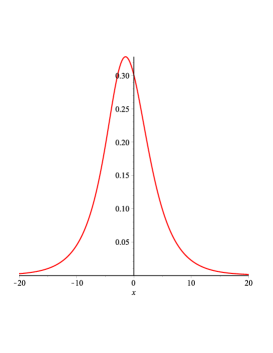
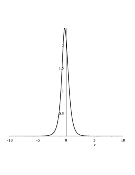
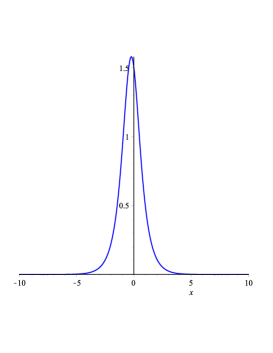
Figure 3: 1-soliton-like solution as n=1. $\lambda_{1}(0)=1+i$, $\widetilde{\lambda}_{1}(0)=2-i$, $c_{1}(0)=\lambda_{1}(0)^{2}$, $\widetilde{c}_{1}(0)=\widetilde{\lambda}_{1}(0)^{2}$. (a): $t=-1$; (b): $t=0$; (c): $t=1$;

5. Conclusion

In this paper, we introduced a systematic approach to solve the initial value problem associated with the non-isospectral TD hierarchy through the utilization of the inverse scattering transform. Given our consideration of the non-isospectral case, we acquired the time evolution of the scattering data, which is different from that of the corresponding isospectral TD hierarchy. Finally, we obtained the exact solutions of this hierarchy under various parameters. Moreover, these exact solutions can also be verified by substituting them into the corresponding equations. There are several problems to be considered in the future. How to research rogue waves of equations presented in the paper in terms of the approach [26, 27].

Data Availability

Data sharing is not applicable to this article as no new data were created or analyzed in this study.

References

- [1] C.S. Gardner, J.M. Green, M.D. Kruskal, R.M. Miura, Method for solving the Korteweg-de Vries equation, Phys. Rev. Lett., 19 (1967) 1095-1097.
- [2] V.E. Zakharov, S.V. Manakov, S.P. Novikov and L.P. Pitaevskii 1984 Theory of Solitons: The Inverse Scattering Method (New York: Consultants Bureau).
- [3] M.J. Ablowitz, H. Segur, Solitons and the inverse scattering transform. Philadelphia, PA: SIAM, 1981.
- [4] M.J. Ablowitz, P.A. Clarkson, Solitons, nonlinear evolution equations and inverse scattering. Cambridge university press, 1991.
- [5] J.L. Ji, Z.N. Zhu, Soliton solutions of an integrable nonlocal modified Korteweg-de Vries equation through inverse scattering transform. J. Math. Anal. Appl. 453 (2017) 973-984.
- [6] W.X. Ma, Riemann-Hilbert problems of a six-component mKdV system and its soliton solutions Acta. Math. Sci. 39 509-23.
- [7] T.K. Ning, D.Y. Chen and D.J. Zhang, The exact solutions for the nonisospectral AKNS hierarchy through the inverse scattering transform. Physica A, 339 (2004) 248-266.
- [8] T.K. Ning, D.Y. Chen and D.J. Zhang, Soliton-like solutions for a nonisospectral KdV hierarchy. Chaos Solitons Fractals, 21 (2004) 395-401.
- [9] Q. Li, D.J. Zhang and D.Y. Chen, Solving the hierarchy of the nonisospectral KdV equation with self-consistent sources via the inverse scattering transform. J. Phys. A Math. Theor.,41 (2008) 355209.
- [10] Q. Li, D.J. Zhang and D.Y. Chen, Solving non-isospectral mKdV equation and Sine-Gordon equation hierarchies with self-consistent sources via inverse scattering transform. Commun. Theor. Phys., 54 (2010) 219.
- [11] Q. Li, D.Y. Chen, J.B. Zhang and S.T. Chen, Solving the non-isospectral Ablowitz-Ladik hierarchy via the inverse scattering transform and reductions. Chaos Solitons Fractals, 45 (2012) 1479-1485.
- [12] Y.F. Zhang, Y.Y. Liu, J.G. Liu, B.L. Feng, New Non-Isospectral Integrable Hierarchy and Some Associated Symmetries, J. Math. Res. Appl., 43 (2023).
- [13] H.F. Wang, Y.F. Zhang, Two Nonisospectral Integrable Hierarchies and its Integrable Coupling, Int. J. Theor. Phys, 59 (2020) 2529-2539.
- [14] H.F. Wang, Y.F. Zhang, Generating of Nonisospectral Integrable Hierarchies via the Lie-Algebraic Recursion Scheme, Mathematics, 8 (2020) 621.
- [15] H.F. Wang, Y.F. Zhang, Generating nonisospectral integrable hierarchies via a new scheme, Adv. Differ. Equ, 170 (2020).
- [16] F. Calogero, A. Degasperis, Exact solution via the spectral transform of a generalization with linearlyx-dependent coefficients of the nonlinear Schrödinger equation, Lett. Nuovo Cimento 22 (1978) 420-424.
- [17] F. Calogero, A. Degasperis, The Spectral Transform and Solitons, North-Holland, Amsterdam, 1982.
- [18] Y.S. Li, A class of evolution-equations and the special deformation, Sci. Scinica A 25 (1982) 911-917.
- [19] W.X. Ma, An approach for constructing nonisospectral hierarchies of evolution equations, J. Phys. A: Math. Gen. 25 (1992) L719.
- [20] W.X. Ma, Lax representations and Lax operator algebras of isospectral and nonisospectral hierarchies of evolution equations, J. Math. Phys. 33 (1992) 2464-2476.
- [21] D.Y. Chen, D.J. Zhang, Lie algebraic structures of (1+1)-dimensional Lax integrable systems, J. Math. Phys. 37 (1996) 5524-5538.
- [22] R. Hirota, J. Satsuma, N-Soliton Solution of the KdV Equation with Loss and Nonuniformity Terms, J. Phys. Soc. Japan 41 (1976) 2141-2142.
- [23] M.R. Gupta, Exact inverse scattering solution of a non-linear evolution equation in a non-uniform medium, Phys. Lett. A 72 (1979) 420-422.
- [24] W.L. Chan, K.S. Li, Nonpropagating solitons of the variable coefficient and nonisospectral Korteweg-de Vries equation, J. Math. Phys. 30 (1989) 2521-2526.
- [25] Y.F. Zhang, H.F. Wang, N.Bai, Schemes for Generating Different Nonlinear Schrödinger Integrable Equations and Their Some Properties, Acta. Math. Appl. Sin, 38 (2022) 579-600.
- [26] H.Y. Zhang, Y. F. Zhang, Analysis on the M-rogue wave solutions of a generalized (3+1)-dimensional KP equation, Appl. Math. Lett., 102 (2020) 106145.
- [27] H.Y. Zhang, Y. F. Zhang, Darboux transformations, multisolitons, breather and rogue wave solutions for a higher-order dispersive nonlinear Schrodinger equation, J. Appl. Anal. Comput., 11 (2021) 892-902.
- [28] G.Z. Tu, The trace identity, a powerful tool for constructing the Hamiltonian structure of integrable systems, J. Math. Phys, 30 (1989) 330-338.
- [29] G.Z. Tu, D.Z. Meng, The trace identity, a powerful tool for constructing the Hamiltonian structure of integrable systems. II, Acta. Math. Appl. Sin-E., 5 (1989) 89-96.
- [30] C.C. Cao, X.G. Geng, Bargmann system and the involutive repersentations of solutions of the TD Hierarchy, Acta. Math. Appl. Sin., 16 (1993) 82-88.
- [31] J.Y. Zhu, X.G. Geng, Miura transformation for the TD hierarchy, Chin. Phys. Lett., 23 (2006) 1-3.
- [32] J.Y. Zhu, L.L. Wang, X.G. Geng, Riemann-Hilbert approach to TD equation with nonzero boundary condition, Front. Math. China, 13 (2018) 1245-1265.
- [33] J.Y. Zhu, L.L. Wang, Kuznetsov-Ma solution and Akhmediev breather for TD equation, Commun. Nonlinear. Sci. Numer. Simul., 67 (2019) 555-567.
- [34] M. Lakshmanan, Continuum spin system as an exactly solvable dynamical system, Phys. Lett. A 61 (1977) 53-54.
- [35] L.A. Takhtajan, Integration of the continuous Heisenberg spin chain through the inverse scattering method, Phys. Lett. A 64 (1977) 235-237.
- [36] Z.J. Qiao, A finite-dimensional integrable system and the involutive solutions of the higher-order Heisenberg spin chain equations, Phys. Lett. A 186 (1994) 97-102.
- [37] X.G. Geng, X. Zeng, B. Xue, Algebro-geometric solutions of the TD hierarchy, Math. Phys. Anal. Geom., 16 (2013) 229-251.
- [38] H.Y. Zhang and Y.F. Zhang, Spectral analysis and long-time asymptotics of complex mKdV equation, J. Math. Phys., 63 (2022), 021509.