Scale-free networks: Improved Inference

Abstract

The power-law distribution plays a crucial role in complex networks as well as various applied sciences. Investigating whether the degree distribution of a network follows a power-law distribution $x^{-\alpha}$, with $2<\alpha<3$ (scale-free hypothesis), is an important concern. The commonly used inferential methods for estimating the model parameters often yield biased estimates, which can lead to the rejection of the hypothesis that a model conforms to a power-law. In this paper, we discuss improved methods that utilize Bayesian inference to obtain accurate estimates and precise credibility intervals. The inferential methods are derived for both continuous and discrete distributions. These methods reveal that objective Bayesian approaches return nearly unbiased estimates for the parameters of both models. Notably, in the continuous case, we identify an explicit posterior distribution. This work enhances the power of goodness-of-fit tests, enabling us to accurately discern whether a network or any other dataset adheres to a power-law distribution. We apply the proposed approach to fit degree distributions for more than 5,000 synthetic networks and over 3,000 real networks. The results indicate that our method is more suitable in practice, as it yields a frequency of acceptance close to the specified nominal level.

Keywords: Scale-free, power-law, bias correction, goodness-of-fit.

1 Introduction

During his studies of medicine at the University of Pisa in approximately 1580, Galileu Galilei discovered a relationship between an animal’s mass (M) and its size (L, length), represented as $M\approx L^{3}$. He also observed that the scaling of bone area follows $S\approx L^{2}$ [41]. This finding indicates that mass grows at a faster rate than bone area, suggesting that larger animals are less common compared to smaller ones. Galileo’s observation is one of the first examples of a power law, which manifests in numerous natural and artificial systems.

Kepler’s third law, Newton’s law of gravitation, Coulomb’s law of electromagnetism, and Stefan-Boltzmann law are examples of power laws, which can be expressed in the form [32]:

$$f(x)=Cx^{-\alpha},\quad 0<x<\infty,\quad\alpha>0,$$ (2)

where $\alpha$ is called the scaling exponent. The greater the variable $x$ value, the smaller the function $f(x)$ value. In the Newton’s and Coulomb’s laws, $x$ represents the distance between planets or charges, where $\alpha=2$. Thus, the closer two planets or electric charges are, the stronger the force between them. Stokes’ Law, self-organized criticality, and the Curie-von Schweidler Law and and Keibler’s Law, which relates metabolic rate to the mass of an organism, also present this relationship.

The laws of Kepler, Newton, and Coulomb are deterministic models in the sense that we can precisely predict the gravitational or electric force and the position of a planet at any given time. Equation 2 defines a power law generally, not necessarily deterministic. Thus, we can also formulate a power law for stochastic processes. In this case, $f(x)$ represents a probability distribution or a probability density function, if $X$ is a continuous random variable. Power-law distributions can be observed in diverse phenomena, such as the distribution of wealth, where a small percentage of individuals hold the majority of financial resources, the distribution of city sizes, with a few megacities vastly outweighing smaller urban centers, and in online social networks, where a handful of users have an overwhelmingly large number of connections

Due to the inherent stochastic elements in data, establishing the presence of power-law scaling poses a significant challenge. In this context, a pivotal question arises concerning whether a given dataset adheres to a power law distribution. This inquiry holds fundamental significance, as power laws can arise from diverse underlying mechanisms [41]. For instance, power laws are linked to the fractal organization and can emerge through preferential attachment, self-organized criticality, and energy and cost minimization in information transmission [41]. Thus, the identification of a power law in a system is of utmost importance, because it offers valuable insights into the underlying mechanisms that govern the system’s behavior. Furthermore, power laws are closely linked to scale invariance and self-similarity across different scales, providing a framework for prediction, modeling, and decision-making. Power laws also serve as indicators of critical points and phase transitions [39, 40, 41], enabling the identification of thresholds and emergent phenomena. Ultimately, the recognition of power laws enhances our understanding of complex systems, with far-reaching implications in scientific, social, and economic domains [32, 12]. Ultimately, Ramos et al. [35, 36] introduced an extension of this model that incorporates change points to describe piecewise patterns for predicting the time-to-violent-death of Roman and Egyptian emperors.

Power-law identification is also critical when dealing with complex networks [31]. Networks whose number of connections (called degree) follows a power-law distribution are called scale-free networks [14, 3, 5]. Across most classes of networks, it is common to find evidence that the degree distribution of real-world networks [5], such as the World Wide Web [1], biological networks [34, 26], software systems [46], and citation distributions [37], follows a power-law distribution. This distribution is represented by its probability density function (pdf) given as follows:

$$f(x)\propto x^{-\alpha},\quad x>x_{\min}.$$ (3)

where $\alpha$ is a scaling parameter that must be greater than 1, typically falling in the range $2<\alpha<3$ (scale-free hypothesis) [5]. In practice, the power-law applies only to values greater than a minimum value $x_{\min}$, referred to as the lower bound. This is termed as the tail of the distribution and is discussed in [12].

Due to the importance of power law in stochastic systems, recently, a great debate suggested that power-laws are not so common as verified before [7]. Many methods have been proposed to identify power law in data [12]. The most common is based on the maximum likelihood estimation (MLE), but this approach can be heavily biased for small samples [8]. Moreover, MLE is sensitive to outliers, which is critical for power laws distribution, which have long tails, and these outliers can have a disproportionately large effect on the MLE estimate. In addition, in data acquisition, empirical datasets often only cover a narrow range of observation, making it difficult to establish power-law behavior unambiguously. Therefore, determine if a data set follows a power law and infer its parameters is a challenge for traditional statistical methods and new approaches are necessary.

In this paper, we provide a Bayesian approach to address the scale-free issue and propose an unbiased estimator in the continuous and discrete cases to improve the method by Broido and Clauset [7]. We consider the use of an objective prior [23] that leads to an explicit posterior distribution in the continuous case and an efficient estimator in terms of bias and root mean square error (RMSE). Moreover, the obtained posteriors have attractive properties: (i) invariance under one-to-one transformations, (ii) consistency under marginalization, and (iii) good coverage probabilities [25]. We show, through an extensive simulation study, that our proposed estimators return nearly unbiased estimates for the parameters, even for small samples. Hence, our results are more accurate than those obtained by the maximum likelihood method.

Additionally, we address the problem of network classification as a scale-free network. Clauset et al. [12] presented an approach based on the KS statistic to evaluate the goodness of fit. However, our results indicate that as the sample size increases, the proposed test may not return reliable results. We overcome this problem by proposing to use the KS test jointly with the chi-square method. The proposed approach for pseudo-random samples as well as for degree distributions is obtained from the Barabási-Albert model, a network model whose degree distribution has a power-law distribution [30]. Our results suggest that our method is more suitable in practice since it provides a frequency of acceptance close to the nominal level. Our results can have an important impact on many areas of complex networks where the parameter to be estimated is important to check whether or not a network is scale-free.

2 Power law in data

Graphically, the presence of power-law behavior is suggested when we observe a roughly linear decay of points on the plot of the degree distribution using a logarithmic scale on both axes, as opposed to an exponential behavior where a linear decay is not expected. Identifying power-law behavior provides significant theoretical insights into its generative mechanism [44]. This phenomenon appears in stock price fluctuations [16], earthquake magnitudes [2, 24], and tree-limb branching [6].

To fit a power-law distribution to a dataset, parameter estimation is typically conducted using classical methods [12, 19, 45]. The most common approach is the maximum likelihood estimator, which has a simple closed-form expression in the continuous case. However, this estimator exhibits bias with small samples, which is undesirable [8]. In the discrete case, the density function is modified, and the maximum likelihood estimation method lacks a closed-form expression. Although [12] discussed a closed-form approximation for the parameter, both estimators exhibit significant bias, potentially leading to incorrect conclusions.

In the realm of complex networks, Barabási and Albert [4] proposed a model capable of replicating the growth of numerous real networks. In this model, nodes are added one by one to the system with a probability proportional to the number of links existing nodes possess at that time. The networks generated by this model present a power law distribution in the number of connections [30]. Power-law behavior is often observed across various network classes, including the World Wide Web [1], biological networks [34, 26], infectious diseases [17, 33], software systems [46], and citation distributions [37].

In a recent study, Broido and Clauset [7] analyzed over 3000 networks from biological, informational, social, technological, and transportation domains obtained from the Index of Complex Networks [13] to verify the scale-free hypothesis in each case. They employed a standard Kolmogorov-Smirnov (KS) minimization to determine the minimum degree $k_{\mathrm{min}}$, and the maximum likelihood estimator was used to find the exponent of the power-law. The statistical plausibility of the fitted model was assessed using the goodness-of-fit test, and networks were categorized as strong or weak scale-free based on the p-value. Network datasets were classified according to the definition provided in Table 1.

Table 1: Definitions of a scale-free network by [7]

. Super-Weak For at least 50% of graphs, no alternative distribution is favored over the power-law. Weakest For at least 50% of graphs, a power-law distribution cannot be rejected ($p\geq 0{.}1$). Weak Requirements of Weakest, and the power-law region contains at least 50 nodes. Strong Requirements of Weak and Super-Weak, and $2<\alpha<3$ for at least 50% of graphs Strongest Requirements of Strong and Super-Weak for at least 90% and 95% of graphs, respectively. Not Scale Free Networks that are neither Super-Weak nor Weakest.

They conclude that scale-free networks are not commonly observed in natural and artificial systems, contrary to prior knowledge, where power-law degree distributions appear to be ubiquitous in networks across many areas of science [5]. Although Broido and Clauset’s work [7] provided a broad analysis of many networks and raised the scale-free hypothesis, their results have some limitations. Different values for the parameters lead to different classifications as a scale-free network, whereas the estimator generates unnecessary bias. Indeed, when the network size increases, contrariwise to expectation, the goodness-of-fit (GOF) test leads to a loss of power. Moreover, they are limited to a point estimator (under a frequentist approach) and do not allow classification according to a confidence interval, ignoring the uncertainty itself.

3 Continuous Power-Law distribution

Let $X$ be a continuous random variable, $X$ has a power-law distribution if their probability density function (PDF), which is obtained normalizing equation (3), is given by

$$f(x;\alpha)=\frac{\alpha-1}{x_{\min}}\left(\frac{x}{x_{\min}}\right)^{-\alpha},\quad x>x_{\min}.$$ (4)

This function is characterized by a heavy tail, which means that it has a significant probability of observing extreme values. Their cumulative density function (CDF) is

$$F(x;\alpha)=1-\left(\frac{x}{x_{\min}}\right)^{1-\alpha},\quad x>x_{\min}.$$

If $X$ has a power-law distribution then the $r$-th moment is given by

$$E[X^{r}]=\int_{x_{\min}}^{\infty}x^{r}f(x;\alpha)dx=\frac{(\alpha-1)x_{\min}^{r}}{\alpha-1-r},\quad\alpha>r+1.$$

Estimating the parameters in the power-law distribution is an important task in statistical analysis. The estimation of the scaling parameter is usually conducted under the classical approach [12, 19, 45], assuming previously that $x_{\min}$ is known. On the other hand, the estimation of the lower bound is made through the optimization of a goodness-of-fit statistic.

Clauset et al. [12] discuss two approaches to estimate $x_{\min}$. The first one [21] consists in representing the data below of $x_{\min}$ by a separate probability $p_{k}=P(X=k)$ for $1\leq k<x_{\min}$, and above $x_{\min}$ by a power-law distribution. Given that the model cannot be fit directly, as the number of parameters is not fixed, we may maximize the Bayesian information criterion (BIC) given by $BIC=\mathcal{L}-x_{\min}/2\log n$, where $\mathcal{L}$ is the value of the conventional log-likelihood at its maximum. However, this method has some difficulties: the BIC will tend to underestimate $x_{\min}$, which can lead to a biased estimation of the scaling parameter. In addition, it is unclear how this method can be generalized to continuous data.

The second one uses the Kolmogorov-Smirnov (KS) statistic, proposing to take the $x_{\min}$ that makes the probability distributions of the data and the best-fit power-law model as similar as possible above. Mathematically, $\hat{x}_{\min}$ is the value of $x_{\min}$ that minimizes $D$, defined as:

$$D=\max_{x\geq x_{\min}}|S(x)-F(x)|,$$

where $S(x)$ is the CDF of the data for the observations with value at least $x_{\min}$, and $F(x)$ is the CDF for the power-law model that best fits the data in the region $x\geq x_{\min}$. Since the power-law distribution only applies to values above some lower bound, the statistic discards all data below this point. They justify that the last one gives excellent results and generally performs better than the BIC approach [12].

As following, we will explore different approaches to estimating the scaling parameter assuming that the lower bound is known. In Appendix A, B, and C, some estimation methods are presented under a classical inference approach. Next, we consider a Bayesian inference approach and present the results of a simulation study to compare the performance of each estimator.

3.1 Bayes Estimator

Inferential procedures using Bayesian methods have become popular in the past few decades [43]. Under the Bayesian approach, the parameter is treat as random variable and a prior distribution $\pi(\alpha)$ is assumed to represent the objective or subjective beliefs about $\alpha$. The posterior distribution for $\alpha$, from which inferences are drawn, is proportional to the product of the likelihood function and the prior distribution.

A common prior that allow us to obtain a posterior distribution, where the dominant information is obtained from the data, is known as the Jeffreys prior which has been widely used due to its invariance property under one-to-one transformations of parameters [23]. This prior is obtained from the square root of the Fisher information element in (18) and is given by

$$\pi\left(\alpha\right)\propto\frac{1}{(\alpha-1)}.$$ (5)

The posterior distribution for $\alpha$, produced by the Jeffreys prior, is given by

$$\pi(\alpha\mid\boldsymbol{x})=\frac{1}{d(\boldsymbol{x})}\left(\alpha-1\right)^{n-1}\prod_{i=1}^{n}\left(\frac{x_{i}}{x_{\min}}\right)^{-\alpha}.$$ (6)

Since the prior distribution is an improper distribution, i.e., does not exist a normalizing constant which can be multiplied for the area under the graph of (5) was the unit, its necessary to ensure that (6) was a proper distribution. In fact, we proved that for $n\geq 1$ we have

$$d(\boldsymbol{x})=\int_{1}^{\infty}\left(\alpha-1\right)^{n-1}\prod_{i=1}^{n}\left(\frac{x_{i}}{x_{\min}}\right)^{-\alpha}d\alpha<\infty.$$

In addition, we also prove that all the higher moments converge, i.e, for $r\in\mathbb{N}_{0}$

$$E(\alpha^{r}\mid\boldsymbol{x})=\int_{1}^{\infty}\alpha^{r}\pi(\alpha\mid\boldsymbol{x})d\alpha<\infty,$$

guaranteeing particularly that the posterior expectation exists (see the Appendix D for more details).

Moreover, after a convenient algebraic manipulation, we can identify from (6) that

$$\pi(\alpha\mid\boldsymbol{x})\propto\left(\alpha-1\right)^{n-1}\exp\left(-(\alpha-1)\sum_{i=1}^{n}\log\left(\frac{x_{i}}{x_{\min}}\right)\right),$$

which is a kernel of a Gamma distribution shifted by 1 parameterized in terms of a shape and scale parameters. From above its direct to obtain point estimators or credible intervals.

The first Bayes estimator that will be considered is the the posterior mode also know as maximum a posterior probability (MAP), such estimator is obtained by considering the maximum of the posterior distribution. In this case, the MAP is given by

$$\hat{\alpha}_{\operatorname{MAP}}=1+(n-1)\left(\sum_{i=1}^{n}\log\left(\frac{x_{i}}{x_{\min}}\right)\right)^{-1}.$$

Another common Bayes estimator is the expectation posterior (EP), usually used due to its good properties such as its optimality under the Kullback-Leibler divergence [29]. The EP is given by

$$\hat{\alpha}_{\operatorname{EP}}=1+n\left(\sum_{i=1}^{n}\log\left(\frac{x_{i}}{x_{\min}}\right)\right)^{-1}.$$

For one parameter case the credible interval for $\alpha$ has a coverage error $O$($n^{-1}$) in the frequentist sense (see Tibshirani [42]), i.e.,

$$P\left[\alpha\leq\theta_{1-\gamma}\mid\boldsymbol{x}\right]=1-\gamma-\mathcal{O}(n^{-1}),$$ (7)

where $\theta_{1-\gamma}$ denote the $(1-\gamma)$-th quantile of the posterior distribution of $\alpha$. The class of priors satisfying (7) are known as matching priors.

3.2 Simulation Study

In this section, we compare the proposed estimators for the scale parameter based on bias, root-mean-square error (RMSE), and coverage probabilities (CP). The first two metrics are computed as follows:

$$\operatorname{Bias}(\alpha)=\frac{1}{N}\sum_{i=1}^{N}(\hat{\alpha}_{i}-\alpha),\quad\operatorname{RMSE}(\alpha)=\sqrt{\sum_{i=1}^{N}\frac{(\hat{\alpha}_{i}-\alpha)^{2}}{N}},$$

where $N=5,000$ represents the number of estimations (or replicates) obtained for a unique sample size generated by the inverse transform sampling (see Appendix E).

The most efficient estimation method will return a bias closer to zero with smaller RMSEs. Additionally, we specify a 95% confidence (credibility) level, i.e., we expect that the frequencies of the intervals that cover the true values of $\alpha$ should be closer to 0.95. These probabilities are computed using the confidence or credibility intervals, as applicable. We did not compute the CP for the moment estimators since confidence intervals were not obtained.

We consider the following estimators for the simulation study: the MLE, ME, MPS, Bayes MAP, and Bayes Mean. Since the CMLE has the same form as the MAP estimator and the MLE the same form as the EP estimator, the bias and RMSE will be the same, and only the CPs will differ, since one is obtained from the posterior distribution and the other from asymptotic theory.

Figures 1-2 display the bias and RMSEs from the estimates of $\alpha$. We can note that both bias and RMSEs, obtained from different estimation methods, tend to zero when $n$ increases. The ME returned the biggest bias among the estimators. The standard MLE and the Bayes estimator obtained from the posterior mean returned similar results. On the other hand, the Bayes MAP, as well as the corrective approach, provided precise estimates even for small sample sizes. Considering the CPs, the Bayes MAP returned better coverage probabilities, especially when compared with the CPs of the CMLE, these results are expected due to the theoretical results related to the matching priors. Overall, these results show that the MAP estimator obtained from the Bayesian approach should be considered for estimating the scale parameter of the power-law distribution.

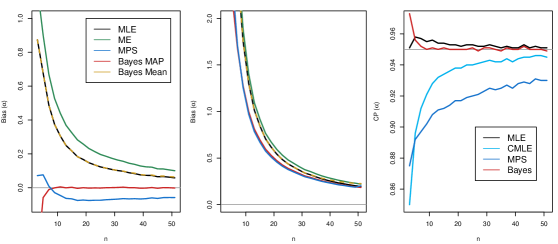
Figure 1: Performance of the estimators in terms of Bias (left), RMSEs (middle), and CP (right) using random samples of sizes $n=(4,6,\ldots,50)$ generated from a power-law distribution with $x_{\min}=1$ and $\alpha=4$.

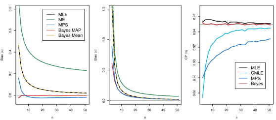
Figure 2: Performance of the estimators in terms of Bias (left), RMSEs (middle), and CP (right) using random samples of sizes $n=(4,6,\ldots,50)$ generated from a power-law distribution with $x_{\min}=0.5$ and $\alpha=2$.

4 Discrete power-law distribution

The power-law behavior can be extended to the discrete case adapting (3) to get a probability mass function (PMF). This has an important background since the degree distribution of a network is registered on a discrete scale. Let $X$ be a discrete random variable, $X$ has a power-law distribution if their PMF is

$$p(x;\alpha)=\frac{x^{-\alpha}}{\zeta(\alpha,x_{\min})},$$ (8)

where $\zeta(\alpha,x_{\min})$ is the Hurwitz zeta function defined by

$$\zeta(\alpha,x_{\min})=\sum_{n=0}^{\infty}\left(n+x_{\min}\right)^{-\alpha},$$ (9)

We will explore different approaches to estimating the scaling parameter. This goal its important because to use the estimators for the continuous case in the discrete model will lead to biased estimates [12]. In the end, we will analyze the performance of each estimator through of a simulation study.

4.1 Maximum Likelihood Estimation

Let $X_{1},\ldots,X_{n}$ be a random sample such that $X$ has PMF given in (8), the log-likelihood function is

$$\ell(\alpha;\boldsymbol{x})=-n\log\zeta(\alpha,x_{\min})-\alpha\sum_{i=1}^{n}\log(x_{i}).$$ (10)

The MLE can be found solving the equation

$$\frac{\zeta^{\prime}(\alpha,x_{\min})}{\zeta(\alpha,x_{\min})}=-\frac{1}{n}\sum_{i=1}^{n}\log(x_{i}).$$ (11)

Clauset et al. [12] gets an approximate expression of the MLE by continuity correction, proving that

$$\zeta\left(\alpha,x_{\min}\right)=\frac{\left(x_{\min}-\frac{1}{2}\right)^{-\alpha+1}}{\alpha-1}\left[1+\mathcal{O}\left(x_{\min}^{-2}\right)\right].$$ (12)

Differentiating this expression with respect to $\alpha$, the ratio of zeta functions can be re-expressed by

$$\frac{\zeta^{\prime}\left(\alpha,x_{\min}\right)}{\zeta\left(\alpha,x_{\min}\right)}=-\left[\frac{1}{\alpha-1}+\log\left(x_{\min}-\frac{1}{2}\right)\right]\left[1+\mathcal{O}\left(x_{\min}^{-2}\right)\right]$$

Using this approximation and considering the neglected quantity of order $x_{\min}^{-2}$, we obtain

$$\hat{\alpha}_{\operatorname{MLE}}\approx 1+n\left(\sum_{i=1}^{n}\log\left(\frac{x_{i}}{x_{\min}-\frac{1}{2}}\right)\right)^{-1},$$ (13)

which is identical to the MLE for the continuous case except for the $1/2$ in the denominator. They prove that (13) is a good approximation when $x_{\min}>6$ according to simulations.

Since (11) have not closed-form expression, it need to be solved numerically by functions that found the root of an expression. The Fisher information element in the discrete case is given by

$$\mathcal{I}(\alpha)=-E\left[\frac{\partial^{2}\ell(\alpha;\boldsymbol{x})}{\partial\alpha^{2}}\right]=\frac{\zeta^{\prime\prime}(\alpha,x_{\min})}{\zeta(\alpha,x_{\min})}-\frac{\zeta^{\prime}(\alpha,x_{\min})^{2}}{\zeta(\alpha,x_{\min})^{2}}.$$ (14)

Moreover, using the approximated MLE we can also obtain an approximated Fisher information element for the estimator

$$\mathcal{I}^{-1}(\alpha)\approx\frac{(\alpha-1)^{2}}{n}.$$

4.2 Bayesian Estimator

Under the Bayesian approach, we also consider the Jeffreys prior as objective prior for the parameter of the discrete power-law distribution. In this case, using the element of the Fisher information (14) the Jeffreys prior is given by

$$\pi\left(\alpha\right)\propto\sqrt{\frac{\zeta^{\prime\prime}(\alpha,x_{\min})}{\zeta(\alpha,x_{\min})}-\frac{\zeta^{\prime}(\alpha,x_{\min})^{2}}{\zeta(\alpha,x_{\min})^{2}}}=\sqrt{\phi^{(2)}(\alpha,x_{\min})}$$ (15)

where $\phi^{(i)}(\alpha,x_{\min})$ is the $i$-th derivate of $\log\zeta(\alpha,x_{\min})$.

The posterior distribution for $\alpha$, produced by the Jeffreys prior, is given by

$$\pi(\alpha\mid\boldsymbol{x}) =\frac{1}{d(\boldsymbol{x})}\frac{\sqrt{\phi^{(2)}(\alpha,x_{\min})}}{\zeta(\alpha,x_{\min})^{n}}\prod_{i=1}^{n}x_{i}^{-\alpha}.$$ (16)

Here, the objective prior distribution is also an improper function, therefore, the posterior distribution need to be checked to avoid improper posterior. In this case, the obtained posterior is a proper distribution for $n\geq 1$ as we have

$$d(\boldsymbol{x})=\int_{1}^{\infty}\frac{\sqrt{\phi^{(2)}(\alpha,x_{\min})}}{\zeta(\alpha,x_{\min})^{n}}\prod_{i=1}^{n}x_{i}^{-\alpha}d\alpha<\infty.$$

The proof of the statement above can be seen in detail in Appendix D. For the discrete distribution the posterior moments for the parameters are also finite, i.e.,

$$E(\alpha^{r}\mid\boldsymbol{x})=\int_{1}^{\infty}\alpha^{r}\pi(\alpha\mid\boldsymbol{x})d\alpha<\infty,\quad r\in\mathbb{N}.$$

In the continuous case, we have showed that the MAP estimator is equivalent to a bias corrected MLE which returned improved estimates for $\alpha$. In order to obtain the MAP estimator for the discrete case we have to solve the following non-linear equation

$$\frac{\zeta^{\prime}(\alpha,x_{\min})}{\zeta(\alpha,x_{\min})}-\frac{1}{2n}\frac{\partial^{2}\log\left(\phi^{(2)}(\alpha,x_{\min})\right)}{\partial\alpha^{2}}=-\frac{1}{n}\sum_{i=1}^{n}\log(x_{i}).$$

Solving directly the equation above is not an easy task specially because it is difficult to obtain the second derivate of $\log\left(\phi^{(2)}(\alpha,x_{\min})\right)$. The direct maximization of the logarithm of the posterior distribution is more simple, i.e., we have to maximize the following equation

$$\log(\pi(\alpha\mid\boldsymbol{x}))=0.5\log\left(\phi^{(2)}(\alpha,x_{\min})\right)-n\log\zeta(\alpha,x_{\min})-\alpha\sum_{i=1}^{n}\log(x_{i}).$$

Although most mathematical and statistical software does not have the derivatives of the Hurwitz zeta function implemented, we can consider its relationship with the zeta function to obtain such derivatives and calculate $\phi^{(2)}(\alpha,x_{\min})$. The derivatives can be expressed as

$$\zeta^{\prime}(a,x_{\min}) =\zeta^{\prime}(a)+\sum_{k=1}^{x_{\min}-1}\frac{\log(k)}{k^{a}},$$

$$\zeta^{\prime\prime}(a,x_{\min}) =\zeta^{\prime\prime}(a)-\sum_{k=1}^{x_{\min}-1}\frac{\log(k)^{2}}{k^{a}}.$$

There are situations where the implementation of theses derivates may be difficult. Under these scenarios, we can consider that the Jeffreys prior obtained from the continuous models (5) is a good approximation of the Jeffreys prior in the discrete model (see Figure 3).

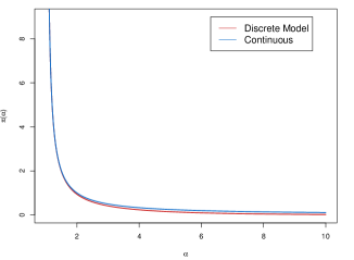
Figure 3: Jeffreys priors for the discrete and continuous case taking $x_{\min}=1$.

The posterior distribution for $\alpha$, produced by the Jeffreys prior in (5), is given by

$$\pi(\alpha\mid\boldsymbol{x}) =\frac{1}{d(\boldsymbol{x})}\frac{(\alpha-1)^{-1}}{\zeta(\alpha,x_{\min})^{n}}\prod_{i=1}^{n}x_{i}^{-\alpha}.$$ (17)

The obtained posterior is also a proper distribution for $n\geq 1$ as we have

$$d(\boldsymbol{x})=\int_{1}^{\infty}\frac{(\alpha-1)^{-1}}{\zeta(\alpha,x_{\min})^{n}}\prod_{i=1}^{n}x_{i}^{-\alpha}d\alpha<\infty.$$

The direct maximization can be considered to obtain the MAP estimator while the credibility intervals are obtained from the integration of the posterior distribution.

4.3 Markov chain Monte Carlo maximum likelihood estimator

The MCMC maximum likelihood estimator is a statistical method used to estimate the parameters of a complex statistical model, that it combines the principles of maximum likelihood estimation with Markov chain Monte Carlo methods. Note that, the optimization of the log-likelihood in (10) is equivalent to optimize of the logarithm of the likelihood ratio for an arbitrary and fixed $\alpha_{0}$,

$$\ell(\alpha;\boldsymbol{x})-\ell(\alpha_{0};\boldsymbol{x}) =-(\alpha-\alpha_{0})\sum_{i=1}^{n}\log(x_{i})-n\log\left(\dfrac{\zeta(\alpha,x_{\min})}{\zeta(\alpha_{0},x_{\min})}\right),$$

$$=-(\alpha-\alpha_{0})\sum_{i=1}^{n}\log(x_{i})-n\log\left[\sum_{x=x_{\min}}^{\infty}\dfrac{x^{-\alpha}}{\zeta(\alpha_{0},x_{\min})}\right],$$

$$=-(\alpha-\alpha_{0})\sum_{i=1}^{n}\log(x_{i})-n\log\left[\sum_{x=x_{\min}}^{\infty}x^{-(\alpha-\alpha_{0})}p(x;\alpha_{0})\right],$$

$$=-(\alpha-\alpha_{0})\sum_{i=1}^{n}\log(x_{i})-n\log\left[E_{\alpha_{0}}\left(X^{-(\alpha-\alpha_{0})}\right)\right].$$

Replacing the expectation with random variables $t_{1},\ldots,t_{m}$ independent and identically distributed to $p(x;\alpha_{0})$, we can obtain an approximated expression for the likelihood ratio whose maximum value is at the same time an approximation of the MLE

$$\widehat{\alpha}_{m}=\underset{\alpha>1}{\operatorname{arg}\max}\ \left\{-(\alpha-\alpha_{0})\sum_{i=1}^{n}\log(x_{i})-n\log\left(\dfrac{1}{m}\displaystyle\sum_{j=1}^{m}t_{j}^{-(\alpha-\alpha_{0})}\right)\right\}.$$

Geyer [18] proves that if the chain $T_{1},...,T_{m}$ is irreducible, then

$$\dfrac{1}{m}\displaystyle\sum_{j=1}^{m}T_{j}^{-(\alpha-\alpha_{0})}\overset{a.s}{\longrightarrow}E_{\alpha_{0}}\left(X^{-(\alpha-\alpha_{0})}\right),$$

in addition, as the power-law distribution belongs to the exponential family when $x_{\min}$ is known, he assures that $\widehat{\alpha}_{m}\overset{a.s}{\longrightarrow}\widehat{\alpha}_{\operatorname{MLE}}$. This inference procedure is widely used in complex statistical models, specifically when we cannot normalize the kernel of a probability distribution, as in the case of the discrete power-law distribution. Instead of maximizing the traditional likelihood function, which will depend on a non-explicit normalization constant, we can maximize an alternative function whose maximum coincides with the maximum of the likelihood function.

The convergence to the MLE is guaranteed, as mentioned above, however, the speed of convergence will depend on the chosen value to $\alpha_{0}$ and consequently on the large of the chain $m$, which is typically generated by the Metropolis-Hastings algorithm. This algorithm constructs a Markov chain by proposing new values based on a proposal distribution and accepting or rejecting these proposals based on an acceptance probability. The acceptance probability is determined by comparing the likelihoods of the proposed and current values. In our case, we will not perform this method in the simulation study.

4.4 Simulation Study

We have discussed different possible estimators, under the same considerations of Section 3.2. The number of estimates $N=5,000$ are obtained through the MLE, CMLE, AMLE, Bayes Exact (obtained from the MAP), and Bayes Approximated (computed from the MAP of the posterior distribution (17)). The CP for the Bayes estimators since confidence intervals were not obtained. The Bayes estimates are obtained from the maximization of the logarithm of the posterior distributions. Since the CMLE has the same form as the MAP estimator, the Bias, and the RMSE are the same and will be presented as Bayes MAP, only the CPs differ since one is obtained from the posterior distribution and the other from asymptotic theory. The most efficient estimation method will return the Bias closer to zero with smaller RMSEs.

The pseudo-random samples from a discrete power-law distribution can be generated from the quantile function which is already implemented in the poweRlaw package available in R. Figures 1-2 displays the Bias and the RMSEs from the estimates of $\alpha$ obtained using the MC method. The horizontal lines in the figures correspond to Bias and RMSEs being one and zero respectively.

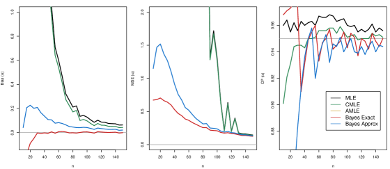
Figure 4: Performance of the estimators in terms of Bias (left), RMSEs (middle), and CP (right) using random samples of sizes $n=(10,\ldots,150)$ generated from a power-law distribution with $x_{\min}=1$ and $\alpha=4$.

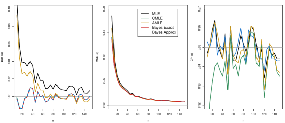
Figure 5: Performance of the estimators in terms of Bias (left), RMSEs (middle), and CP (right) using random samples of sizes $n=(10,\ldots,150)$ generated from a power-law distribution with $x_{\min}=4$ and $\alpha=2$.

As shown in Figures 4-5, both Bias and RMSEs obtained from the different estimation methods tend to zero when $n$ increases. Similar to the continuous case we observed that MLE has the biggest Bias among the estimators. On the other hand, the exact Bayes estimator using the Jeffreys prior provided precise estimates, especially for samples higher than 30. It is worth mentioning that, as $x_{\min}$ increases the Bayes estimator obtained from both priors tends to return similar results. Although the AMLE returns good estimates as $x_{\min}$ increase, the estimator returns poor estimates, especially for small and moderate values of $x_{\min}$ and $n$. However, Considering the CPs, the Bayes MAP returned better coverage probabilities especially when compared with the CPs of the CMLE, these results are expected due to the theoretical results related to the matching priors. Overall, these results show that the MAP estimator obtained from the Bayesian approach should be considered for estimating the scale parameter of the power-law distribution.

5 Testing power-law distribution

There are different approaches that can be used to check the goodness of the fit for a particular distribution (see Huber-Carol et al. [22] and the references therein). For continuous distributions, many tests have already been implemented in different statistical software for general families of distributions [20]. Recently, Chu et al. [10] reviewed over twenty tests for the continuous power-law distribution and concluded the Kolmogorov-Smirnov (KS) returned better results when compared with other goodness of fit (GoF) tests. Hence, our approach should be considered for estimating the parameter of the distribution while the KS test should be used as a GoF test.

In the case of discrete data, some care must be taken. The GoF tests cited by Chu et al. [10] cannot be used in discrete data without modifications. For the discrete power-law distribution, Clauset et al. [12] discussed an approach based on the Kolmogorov-Smirnov (KS) statistics and bootstrap techniques to evaluate the goodness of the fit. The cited approach is advantageous to fit not only data that they came from a pure power-law, but datasets which part of the observations also came from a non-power-law distribution. Before we discuss this important issue, firstly we will focus on providing a GoF test that can be used to select data where the model follows a pure discrete power-law distribution. Hence, we start sampling from the target distribution, then the parameter is estimated under the Bayesian approach, and the KS test with bootstrap is used to check the goodness of the fit, $x_{\min}$ is a fixed known parameter, while the number of replications in the bootstrap was 500. Hereafter, this test will be named as a standard KS test. It is interesting to note that even considering an estimate with less bias we observed that as $n$ increase the power of the test decrease, which is undesirable, such problem was also observed by Klaus et al. [27]. To overcome this problem, we proposed to use jointly the chi-square test and standard Ks test using our Bayesian estimate, in this case, the data follow the target distribution if at least one of the tests returned the p-value higher than $0.05$. The details about the chi-square test are given in Appendix F.

We consider the well-know Barabási-Albert model to generate random scale-free networks using a preferential attachment mechanism. The distribution of the degrees for BA model is a scale-free distribution that follows power-law with $\alpha$ and $x_{\min}$ unknown that needs to be estimated. The function plpnew presented in the Supplemental Material is used to estimate $\alpha$ using the proposed Bayesian approach as well as $x_{\min}$ using the KS approach discussed by [12]. The function barabasi.game was used to generate the networks using the igraph package. The chosen values for the average degree of the network are 4, 5, 6, 7, 8, and 9, while the number of nodes is given by $n=(10,30,\ldots,2000)$. Under this approach, we sample a random BA network, then we estimate the parameters related to the degree distribution as well as the GoF tests assuming a significance level of $5\%$. The distribution follows a power-law distribution if the obtained values are higher than 0.05. Figure 6 present the frequencies of the values that was accepted a power-law model under different average degree.

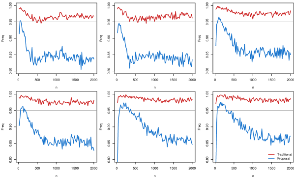
Figure 6: The frequency of Barabási-Albert’s networks selecting properly the target distribution under the standard KS (blue line) and the proposed test (red line). The six specified scenarios for the average grade are displayed from left to right, from top to bottom.

As can be seen, the standard KS introduced by Clauset et al. discriminate correctly the samples for small and moderate samples. This test takes into account an important problem that eliminates part of the sample that does not follow a pure power-law model, including such values in the analysis returned biased estimates. However, similar to the case sample directly from a discrete power-law distribution, as $n$ increase the power of the test decrease. The proposed approach improve decrease the number of reject values for the different average degree returning the frequency of acceptance close to nominal level 0.95. Hence, our proposed approach should be used to test the goodness-of-fit for power-law distributions.

6 Complex networks

We apply our proposal methodology to the same corpus of real-world networks used in Clauset et al. [11] from the ICON [13]. In Table 2 we show that the most networks exhibiting a degree sequence power-law distributed with the current and proposed goodness-of-fit testing. Analyzing these results in depth, we found that over 90% of the networks where the goodness-of-fit methodologies give different results have a lower than average grade (5542). This is consistent with the power improvement observed in our simulation studies for small networks.

Table 2: Number of networks that are scale-free with the current and the proposal goodness-of-fit.

		Proposal
		No	Yes
Actual	No	997	345
	Yes	1	2324

We draw the size of networks analyzed in this study and their respectively mean degree in Figure 7 to distinguish which of them, according to our methodology, have a degree sequence power-law distributed. In addition, we plot in Figure 8 the scaling parameter estimated with the bias corrected estimator, note that the most are scale-free networks.

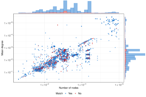
Figure 7: Mean degree of all analyzed networks as a function of the number of nodes. Remarking out those where the goodness-of-fit methodologies give different results.

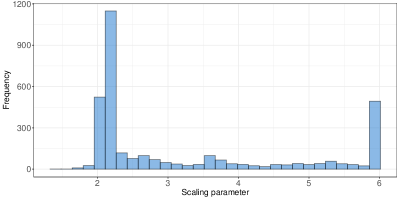
Figure 8: Histogram of the estimated scaling parameter for degree sequences power-law distributed.

Finally, Figure 9 compares the p-values obtained by both methodologies; the traditional goodness-of-fit test and the proposed test. These results are consistent with previous evidence of a greater acceptance of power-law behavior to explain the degree distribution of these networks.

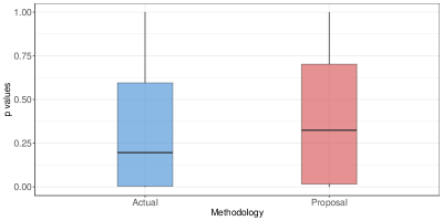
Figure 9: Comparison of results between the traditional goodness-of-fit test (left) and the proposed test (right).

7 Conclusions

We have proposed new estimation methods for the unknown parameters related to power-law distribution with continuous or discrete data. From the continuous case, we proposed a Bayesian estimator using an objective Jeffreys prior that lead to unbiased estimates for the parameter. A simulation study conducted showed that the Bayesian method is very efficient to find accurate estimates as well as credibility intervals. Additionally, the obtained estimator should be used with the KS test to check the goodness of the fit in empirical data.

When the data follow a discrete distribution, we derived different estimators assuming both classical and Bayesian methods. The formal results and proofs are discussed such as the formal expression of the Bias, the proper property of the posterior distributions, and the related higher-order moments. The exact Bayes estimator and its respective credibility intervals have been analyzed by performing simulations that returned precise estimates even for small sample sizes. More importantly, the results outperform the previous estimation procedures used in the literature.

In principle, estimating the parameters of the model is only part of the inferential processes. It is also important to validate the adjusted distribution, i.e., verify when empirical data can be described by a discrete power-law distribution. Hence, we use the proposed estimation method with a GoF test, since the KS test with bootstrap may not return reliable results for large samples. We use the test jointly with the chi-square test, which improves the power of the GoF test. The improved approach is applied to synthetic data generated from a power-law model. Finally, we apply our approach to fit degree distributions for more than 5,000 synthetic networks and over 3,000 real networks. The results indicate that our method is more suitable in practice than the previous approaches, since it provides the frequency of acceptance close to the specified nominal level.

Software

The software R (R Core Development Team) was used to conduct this simulation study. The codes implemented in this work are available under request.

Appendix A Classic inference

A.1 Moments Estimator

The method of moments is one of the simplest estimation procedures which, for one parameter distribution, can be obtained by equating the first theoretical moment with the sample mean, in our case:

$$\frac{(\alpha-1)x_{\min}}{\alpha-2}=\bar{x},$$

where $\bar{x}$ is the empirical mean. Note that, the solution has closed-form expression and is given by

$$\hat{\alpha}_{\operatorname{ME}}=\frac{x_{\min}-2\bar{x}}{x_{\min}-\bar{x}}.$$

However, the estimator above only exists when $\alpha>2$, so it is not advisable to use in general.

A.2 Maximum Likelihood Estimation

The maximum likelihood estimation (MLE) is the most common inferential procedure used to estimate the scale parameter and is obtained by maximizing the likelihood function. The estimator has many attractive properties, such as, invariance, consistent and asymptotically efficient [28].

Let $X_{1},\ldots,X_{n}$ be a random sample such that $X$ has PDF given in (4), then the likelihood function is given by

$$L(\alpha;\boldsymbol{x})=\left(\frac{\alpha-1}{x_{\min}}\right)^{n}\prod_{i=1}^{n}\left(\frac{x_{i}}{x_{\min}}\right)^{-\alpha}.$$

The log-likelihood function, obtained by the logarithm of the likelihood function, is given by

$$\ell(\alpha;\boldsymbol{x})=n\log(\alpha-1)-n\log(x_{\min})-\alpha\sum_{i=1}^{n}\log\left(\frac{x_{i}}{x_{\min}}\right),$$

and their gradient function by

$$\dfrac{\partial\ell(\alpha;\boldsymbol{x})}{\partial\alpha}=\frac{n}{\alpha-1}-\sum_{i=1}^{n}\log\left(\frac{x_{i}}{x_{\min}}\right).$$

Hence, the MLE is easily obtained in closed-form expression

$$\hat{\alpha}_{\operatorname{MLE}}=1+n\left(\sum_{i=1}^{n}\log\left(\frac{x_{i}}{x_{\min}}\right)\right)^{-1}.$$

The MLE is asymptotically normal distributed to $\hat{\alpha}\sim N(\alpha,\mathcal{I}^{-1}(\alpha))\mbox{ for }n\to\infty$, where $\mathcal{I}^{-1}(\alpha)$ is the inverse Fisher information element given by

$$\mathcal{I}^{-1}(\alpha)=-E\left[\frac{\partial^{2}\ell(\alpha;\boldsymbol{x})}{\partial\alpha^{2}}\right]=\frac{(\alpha-1)^{2}}{n}.$$ (18)

Appendix B MLE bias correction

The MLEs for a statistical model are known to exhibit bias of the order $\mathcal{O}(n^{-1})$ (see Cox and Snel [15]). The Cox-Snell methodology can be used to correct for the expected bias and to improve the precision of the estimator. Let $\ell(\boldsymbol{\theta};\boldsymbol{x})$ be the log-likelihood function with a $p$-dimensional vector of parameters $\boldsymbol{\theta}$. The joint cumulants of the derivatives of $\log L(\boldsymbol{\theta};\boldsymbol{x})$ can be written by:

$$h_{ij}(\boldsymbol{\theta}) =E\left(\frac{\partial^{2}\ell(\boldsymbol{\theta};\boldsymbol{x})}{\partial\theta_{i}\theta_{j}}\right),$$

$$h_{ijl}(\boldsymbol{\theta}) =E\left(\frac{\partial^{3}\ell(\boldsymbol{\theta};\boldsymbol{x})}{\partial\theta_{i}\partial\theta_{j}\partial\theta_{l}}\right),$$

$$h_{ij,l}(\boldsymbol{\theta}) =E\left(\frac{\partial^{2}\ell(\boldsymbol{\theta};\boldsymbol{x})}{\partial\theta_{i}\partial\theta_{j}}.\frac{\partial\ell(\boldsymbol{\theta};\boldsymbol{x})}{\partial\theta_{l}}\right),$$

$$h_{ij}^{(l)}(\boldsymbol{\theta}) =\dfrac{\partial h_{ij}(\boldsymbol{\theta})}{\partial\theta_{l}},$$

Using this expression, Cox and Snell [15] proved that for $\theta_{m}$ can be written by

$$\operatorname{Bias}(\hat{\theta}_{m}) =\sum_{i=1}^{p}\sum_{j=1}^{p}\sum_{k=1}^{p}s_{mi}(\boldsymbol{\theta})s_{jl}(\boldsymbol{\theta})\left(h_{ij,l}(\boldsymbol{\theta})+0.5h_{ijl}(\boldsymbol{\theta})\right)+\mathcal{O}(n^{-2})\,,$$

where $\boldsymbol{\theta}$ is a a vector of size $p$, $s^{ij}$ is the $(i,j)$-th element of the inverse of Fisher’s information matrix.

For the proposed model the Bias of $\alpha$ can be written as

$$\operatorname{Bias}(\alpha) =(-h_{11}(\alpha))^{2}\left(h_{11}^{(1)}(\alpha)-\frac{1}{2}h_{111}(\alpha)\right)$$

$$=\frac{(\alpha-1)^{4}}{n^{2}}\left(\frac{2n}{(\alpha-1)^{3}}-\dfrac{1}{2}\frac{2n}{(\alpha-1)^{3}}\right)$$

$$=\frac{\alpha-1}{n}+\mathcal{O}(n^{-2}).$$

Hence, removing the additional bias of the MLE, we have

$$\hat{\alpha}_{\operatorname{CMLE}} =\hat{\alpha}_{\operatorname{MLE}}-\operatorname{Bias}(\hat{\alpha}_{\operatorname{MLE}})$$

$$=1+(n-1)\left(\sum_{i=1}^{n}\log\left(\frac{x_{i}}{x_{\min}}\right)\right)^{-1}.$$

Note that the estimator above can also be seen as a penalized maximum likelihood estimator, where the penalization criteria is given by the logarithm of the square root of the Fisher information element. The logarithm of the penalized likelihood function is given by

$$\ell_{p}(\alpha;\boldsymbol{x}) =\ell(\alpha;\boldsymbol{x})+\log\sqrt{\mathcal{I}(\alpha)},$$

$$=(n-1)\log(\alpha-1)-n\log(x_{\min})-\alpha\sum_{i=1}^{n}\log\left(\frac{x_{i}}{x_{\min}}\right)+\frac{1}{2}\log n.$$

From the equation above, we can obtain the Fisher information element that can be used to construct the confidence interval for the parameter, the element is

$$\mathcal{I}(\alpha)=-E\left[\frac{\partial^{2}\ell_{p}(\alpha;\boldsymbol{x})}{\partial\alpha^{2}}\right]=\frac{n-1}{(\alpha-1)^{2}}.$$

The additional element in the denominator increase the variance of corrected MLE with respect of the MLE, i.e., $Var(\hat{\alpha}_{\operatorname{CMLE}})=\frac{(\alpha-1)^{2}}{n-1}>\frac{(\alpha-1)^{2}}{n}=Var(\hat{\alpha}_{\operatorname{MLE}})$, although in many situation our main aim is to obtain an estimator with smaller variance, we may obtain estimators with poor coverage probabilities. In this case, we will observe that the variance with the denominator $n-1$ improved the coverage probabilities.

Appendix C Method of maximum product of spacings

The maximum product of spacings (MPS) method is an important alternative to MLE for the estimation of unknown parameters of continuous univariate distributions. Proposed by Cheng and Amin [9] this method has desirable properties such as asymptotic efficiency, invariance and more importantly, the consistency of maximum product of spacing estimators holds under more general conditions than for MLEs.

Let $D_{i}(\alpha)=F\left(t_{(i)}\mid\alpha\right)-F\left(t_{(i-1)}\mid\alpha\right)$, for $i=1,2,\ldots,n+1,$ be the uniform spacings of a random sample from the power-law distribution, where $F(t_{(0)}\mid\alpha)=0$ and $F(t_{(n+1)}\mid\alpha)=1.$ Clearly $\sum_{i=1}^{n+1}D_{i}(\alpha)=1$. The maximum product of spacings estimate $\hat{\alpha}_{MPS}$ is obtained by maximizing the geometric mean of the spacings

$$G\left(\alpha\right)=\left[\prod\limits_{i=1}^{n+1}D_{i}(\alpha)\right]^{\frac{1}{n+1}}$$

with respect to $\alpha$, or equivalently, by maximizing the logarithm of the geometric mean of sample spacings

$$H\left(\alpha\right)=\frac{1}{n+1}\sum_{i=1}^{n+1}\log\left(\frac{x_{(i-1)}^{1-\alpha}-x_{(i)}^{1-\alpha}}{x_{\min}^{{}^{1-\alpha}}}\right).$$

The estimate $\hat{\alpha}_{MPS}$ of the parameter $\alpha$ can be obtained by solving the nonlinear equations

$$\frac{1}{n+1}\sum\limits_{i=1}^{n+1}\frac{x_{(i)}^{1-\alpha}\log(x_{(i)})-x_{(i-1)}^{1-\alpha}\log(x_{(i-1)})}{x_{(i-1)}^{1-\alpha}-x_{(i)}^{1-\alpha}}+\log(x_{\min})=0.$$

There may be cases during applications where for some $i$ and $k$ we have that $x_{(i+k)}=\ldots=x_{(i)}$ then $D_{i+k}(\alpha)=\ldots=D_{i}(\alpha)=0$. This implies that the MPS estimator is sensitive to closely spaced observations, especially ties. If ties are observerd, then $D_{i}(\alpha)$ should be replaced by $f(t_{(i)},\alpha)$ as $t_{(i)}=t_{(i-1)}$. The MPS estimator is asymptotically normal distributed with a normal distribution given by

$$\hat{\alpha}_{\operatorname{MPS}}\sim N\left[\alpha,\mathcal{I}^{-1}(\alpha)\right]\mbox{ as }n\to\infty,$$

where $\mathcal{I}^{-1}(\alpha)$ is given by (18). Using the same approach of the MLEs we can construct confidence intervals using the MPS estimator.

Appendix D Some properties

Here we discuss the main proofs related to the posterior distributions discussed in Sections LABEL:secconpl and LABEL:secconpl. Firstly we provide the proof for the continuous case.

Proposition D.1.

For all $r\geq 0$ and $n\geq 1$ we have that

$$E_{\alpha}^{r}[\pi(\alpha|\boldsymbol{x})]=\int_{1}^{\infty}\alpha^{r}\left(\alpha-1\right)^{n-1}\prod_{i=1}^{n}\left(\frac{x_{i}}{x_{\min}}\right)^{-\alpha}\,d\alpha<\infty.$$

Proof.

Indeed, since $(\alpha-1)^{n-1}\leq\alpha^{n-1}$ for all $\alpha\in[1,\infty)$ and $n\geq 1$ it follows that

$$E_{\alpha}^{r}[\pi(\alpha|\boldsymbol{x})]= \int_{1}^{\infty}\alpha^{r}\left(\alpha-1\right)^{n-1}\prod_{i=1}^{n}\left(\frac{x_{i}}{x_{\min}}\right)^{-\alpha}\,d\alpha$$

$$\leq \int_{1}^{\infty}\alpha^{r+n-1}\prod_{i=1}^{n}\left(\frac{x_{i}}{x_{\min}}\right)^{-\alpha}\,d\alpha$$

$$\leq \int_{0}^{\infty}\alpha^{r+n-1}\prod_{i=1}^{n}\left(\frac{x_{i}}{x_{\min}}\right)^{-\alpha}\,d\alpha.$$

On the other hand since not all $x_{i}$ are equal we have that $\prod_{i=1}^{n}\left(\dfrac{x_{i}}{x_{\min}}\right)^{-\alpha}>1$ and thus $\prod_{i=1}^{n}\left(\dfrac{x_{i}}{x_{\min}}\right)^{-\alpha}=\exp(b)$ where $b=\log\left(\prod_{i=1}^{n}\left(\dfrac{x_{i}}{x_{\min}}\right)^{-\alpha}\right)>0$. Therefore it follows that

$$E_{\alpha}^{r}[\pi(\alpha|\boldsymbol{x})]\leq\int_{0}^{\infty}\alpha^{r+n-1}\exp(-b\alpha)\,d\alpha=\frac{1}{b^{r+n}}\int_{0}^{\infty}b(b\alpha)^{r+n-1}\exp(-b\alpha)\,d\alpha$$

and using the change of variables $\alpha=-b\alpha$ we conclude that

$$E_{\alpha}^{r}[\pi(\alpha|\boldsymbol{x})]\leq\frac{1}{b^{r+n}}\int_{0}^{\infty}u^{r+n-1}\exp(-u)du=\frac{\Gamma(r+n)}{b^{r+n}}<\infty.$$

∎

Now, consider the discrete case. Here, we have an additional complexity in the posterior distribution that involves the study of the behavior of the H zeta function and its higher order derivatives. Before we proceed we should notice that given $\alpha>1$ and $n>0$, since $\lim_{x\to\infty}\frac{\log(x)^{n}x^{-\alpha}}{x^{-\beta}}=0$ for any $1<\beta<\alpha$, by comparison, the series

$$\sum_{n=0}^{\infty}\log(n+x_{\min})^{n}\left(n+x_{\min}\right)^{-\alpha}$$

must converge for any $\alpha>1$ and $n>0$, and thus we can differentiate the series for $\zeta(\alpha,x_{\min})$ and obtain that

$$\zeta^{(n)}(a,x_{\min})\quad=\sum_{n=0}^{\infty}\log(n+x_{\min})^{n}\left(n+x_{\min}\right)^{-\alpha}$$

for all $\alpha>1$ and $n>0$.

Proposition D.2.

Let $\operatorname{g}:(a,b)\to\mathbb{R^{+}}$ and $\operatorname{h}:(a,b)\to\mathbb{R^{+}_{*}}$ be continuous functions on $(a,b)\subset\mathbb{R}$, where $a\in\overline{\mathbb{R}}$ and $b\in\overline{\mathbb{R}}$. Then, in case $\lim_{x\to a}\frac{g(x)}{h(x))}=L_{1}>0$ and $\lim_{x\to b}\frac{g(x)}{h(x)}=L_{2}>0$ it follows that $\int_{a}^{b}\operatorname{g}(x)\,dx\propto\int_{a}^{b}\operatorname{h}(x)\,dx$,

Proposition D.3.

For all $r\geq 0$ and $n\geq 0$ we have that

$$E_{\alpha}^{r}[\pi(\alpha|\boldsymbol{x})]=\int_{1}^{\infty}\alpha^{r}\frac{\sqrt{\phi^{(2)}(\alpha,x_{\min})}}{\zeta(\alpha,x_{\min})^{n}}\prod_{i=1}^{n}x_{i}^{-\alpha}d\alpha<\infty.$$

Proof.

From complex analysis we known that $\zeta(\alpha,x_{\min})$ is a meromohphic function with a simple pole at $\alpha=1$ and no other poles and therefore (see Stein [stein2010complex] pg 74, Theorem 1.2) there exist a $\epsilon>0$ and a non-vanishing analytic function $g(\alpha):(1-\epsilon,1+\epsilon)\rightarrow\mathbb{C}$ such that

$$\zeta(\alpha,x_{\min})=(\alpha-1)^{-1}g(\alpha).$$

Moreover, $\zeta(\alpha,x_{\min})\in\mathbb{R},\forall\alpha\in\mathbb{R}$ and thus $g(\alpha)\in\mathbb{R}$ for all $\alpha\in(1-\epsilon,1+\epsilon)$ as well. Thus, it follows that

$$\lim_{\alpha\rightarrow 1^{+}}\frac{\zeta(\alpha,x_{\min})^{-1}}{\alpha^{-1}(\alpha-1)x_{\min}^{\alpha}}=x_{\min}^{-1}\lim_{\alpha\rightarrow 1^{+}}g(\alpha)^{-1}=x_{\min}^{-1}g(1)^{-1}<\infty$$ (19)

Besides, we have

$$\log\left(\zeta(\alpha,x_{\min})\right)=-\log(\alpha-1)+\log(g(\alpha))$$

for all $\alpha\neq 1$ in $(1-\epsilon,1+\epsilon)$, and since $g(\alpha)$ is non-vanishing, we can take the derivative twice and obtain

$$\phi^{(2)}(\alpha,x_{\min})=\frac{1}{(\alpha-1)^{2}}+\frac{\partial}{\partial\alpha^{2}}\log(g(\alpha))\Rightarrow$$

$$\lim_{\alpha\rightarrow 1^{+}}\frac{\phi^{(2)}(\alpha,x_{\min})}{\alpha^{2}(\alpha-1)^{-2}}=1+\lim_{\alpha\rightarrow 1^{+}}(\alpha-1)^{2}\frac{\partial}{\partial\alpha^{2}}\log(g(\alpha))=1$$

where the last equality follows directly from the fact that $\frac{\partial}{\partial\alpha^{2}}\log(g(\alpha))$ is continuous in $(1-\epsilon,1+\epsilon)$. On the other hand, notice that

$$\zeta(\alpha,x_{\min})=\sum_{n=0}^{\infty}\left(n+x_{\min}\right)^{-\alpha}\Rightarrow$$

$$\lim_{\alpha\rightarrow\infty}\frac{\zeta(\alpha,x_{\min})}{x_{\min}^{-\alpha}}=\lim_{\alpha\rightarrow\infty}\sum_{n=0}^{\infty}\left(\frac{n}{x_{\min}}+1\right)^{-\alpha}=\sum_{n=0}^{\infty}\lim_{\alpha\rightarrow\infty}\left(\frac{n}{x_{\min}}+1\right)^{-\alpha}=1.$$

and since $\lim_{\alpha\to\infty}\alpha^{-1}(\alpha-1)=1$ it follows that

$$\lim_{\alpha\rightarrow\infty}\frac{\zeta(\alpha,x_{\min})^{-1}}{\alpha^{-1}(\alpha-1)x_{\min}^{\alpha}}=1.$$

Analogously, from

$$\zeta^{\prime}(a,x_{\min})=\sum_{n=0}^{\infty}\log(n+x_{\min})\left(n+x_{\min}\right)^{-\alpha}\quad\mbox{}\quad$$ (20)

$$\zeta^{\prime\prime}(a,x_{\min})\quad=\sum_{n=0}^{\infty}\log(n+x_{\min})^{2}\left(n+x_{\min}\right)^{-\alpha}$$

we obtain

$$\lim_{\alpha\rightarrow\infty}\frac{\zeta^{\prime}(\alpha,x_{\min})}{x_{\min}^{-\alpha}}=\log(x_{\min})\quad\mbox{ and }\quad\lim_{\alpha\rightarrow\infty}\frac{\zeta^{\prime\prime}(\alpha,x_{\min})}{x_{\min}^{-\alpha}}=\log(x_{\min})^{2}\ .$$

Hence, since $\lim_{\alpha\to\infty}\alpha^{2}(\alpha-1)^{-2}=1$ we conclude that

$$\lim_{\alpha\rightarrow\infty} \frac{\phi^{(2)}(\alpha,x_{\min})}{\alpha^{2}(\alpha-1)^{-2}}=$$

$$=\lim_{\alpha\rightarrow\infty}\frac{\zeta^{\prime\prime}(\alpha,x_{\min})}{x_{\min}^{-\alpha}}\left(\frac{\zeta(\alpha,x_{\min})}{x_{\min}^{-\alpha}}\right)^{-1}-\left(\frac{\zeta^{\prime}(\alpha,x_{\min})}{x_{\min}^{-\alpha}}\right)^{2}\left(\frac{\zeta(\alpha,x_{\min})}{x_{\min}^{-\alpha}}\right)^{-2}$$

$$=\log(x_{\min})^{2}-\log(x_{\min})^{2}=0$$

and thus, from Proposition, there exists $C_{1}>0$ and $C_{2}>0$ such that

$$\zeta(\alpha,x_{\min})^{-1}\leq C_{1}\alpha^{-1}(\alpha-1)x_{\min}^{\alpha}\mbox{ and}$$

$$\phi^{(2)}(\alpha,x_{\min})\leq C_{2}\alpha^{2}(\alpha-1)^{-2}$$

Using these results, it follows that

$$E_{\alpha}^{r}[\pi(\alpha|\boldsymbol{x})] =\int_{1}^{\infty}\alpha^{r}\frac{\sqrt{\phi^{(2)}(\alpha,x_{\min})}}{\zeta(\alpha,x_{\min})^{n}}\prod_{i=1}^{n}x_{i}^{-\alpha}d\alpha$$

$$\leq C_{1}^{n}\sqrt{C_{2}}\int_{1}^{\infty}\alpha^{r-(n-1)}(\alpha-1)^{n-1}\prod_{i=1}^{n}\left(\frac{x_{i}}{x_{\min}}\right)^{-\alpha}d\alpha.$$

Thus, following the sames steps as in Proposition D.1, since $(\alpha-1)^{n-1}\leq\alpha^{n-1}$ for all $\alpha\in[1,\infty)$ and $n\geq 1$, and since $\alpha^{r}\leq 1$ for $r\geq 0$ and $\alpha\geq 1$, and letting $b=\log\left(\prod_{i=1}^{n}\left(\dfrac{x_{i}}{x_{\min}}\right)^{-\alpha}\right)>0$ it follows that

$$E_{\alpha}^{r}[\pi(\alpha|\boldsymbol{x})]\leq C_{1}^{n}\sqrt{C_{2}}\int_{1}^{\infty}\alpha^{r}\prod_{i=1}^{n}\left(\frac{x_{i}}{x_{\min}}\right)^{-\alpha}\,d\alpha$$

$$\leq C_{1}^{n}\sqrt{C_{2}}\int_{0}^{\infty}\alpha^{r}\prod_{i=1}^{n}\exp(-b\alpha)\,d\alpha=C_{1}^{n}\sqrt{C_{2}}\frac{\Gamma(r+1)}{b^{r+1}}<\infty$$

and the proof. ∎

Using the identities proved in Proposition D.3 and following similar steps we observe that

$$E_{\alpha}^{r}[\pi(\alpha|\boldsymbol{x})] =\int_{1}^{\infty}\alpha^{r}\frac{(\alpha-1)^{-1}}{\zeta(\alpha,x_{\min})^{n}}\prod_{i=1}^{n}x_{i}^{-\alpha}d\alpha$$

$$\leq C_{1}^{n}\int_{1}^{\infty}\alpha^{r-n}(\alpha-1)^{n-1}\prod_{i=1}^{n}\left(\frac{x_{i}}{x_{\min}}\right)^{-\alpha}d\alpha$$

$$\leq C_{1}^{n}\int_{0}^{\infty}\alpha^{r-1}\prod_{i=1}^{n}\exp(-b\alpha)d\alpha=C_{1}^{n}\frac{\Gamma(r)}{b^{r}}<\infty$$

and the proof is complete.

Appendix E Simulating Power-Law distribution samples

To generate observations from a power law distribution we consider the Monte Carlo simulations, given in the following algorithm.

Algorithm 1

input $n$, $\alpha$, $x_{\min}$

for  $i=1$ to $n$  do

     $u_{i}\leftarrow U(0,1)$

     $x_{i}\leftarrow x_{\min}\left(1-u_{i}\right)^{1/(1-\alpha)}$

end for

return $x$

Appendix F Chi-squared test

Here we describe the steps to calculate the chi-square test [38]. This test is very useful to asses the goodness of the fit in discrete data. The test is based on the statistic given by

$$\chi^{2}=\sum_{i=1}^{k}\frac{\left(O_{i}-E_{i}\right)^{2}}{E_{i}}$$ (21)

where $O_{i}$ is the observed frequency of the empirical data for the category i and $E_{i}$ is the expected frequency. The number of category $k$ can be chosen from different criteria. To obtain k we considered the observed sample then we group the last components that have only one observed element in one category. This step was used to avoid that extreme values influence the rejection rate. The obtained percentage for the group elements is small and hence the number of categories depends on the sample. Although we have not considered here, another common approach is to group the last components in a category for a fixed percentage (usually around 20%). In our code, if the percentage is not defined we set as standard to used the approach cite earlier. The expected frequencies came from a power-law with the estimated parameter under our approach. Then we use the chisq.test implemented in R to compute the p-value assuming $95\%$ confidence level. If the obtained value is greater the 0.05 we do not reject the null hypothesis that the data came from a power-law distribution.

References

- [1] Réka Albert, Hawoong Jeong, and Albert-László Barabási. Diameter of the world-wide web. nature, 401(6749):130–131, 1999.
- [2] Per Bak, Kim Christensen, Leon Danon, and Tim Scanlon. Unified scaling law for earthquakes. Physical Review Letters, 88(17):178501, 2002.
- [3] Albert-László Barabási. Scale-free networks: a decade and beyond. Science, 325(5939):412–413, 2009.
- [4] Albert-László Barabási and Réka Albert. Emergence of scaling in random networks. science, 286(5439):509–512, 1999.
- [5] Albert-László Barabási. Network science. Cambridge University Press, Cambridge, 2016.
- [6] Lisa Patrick Bentley, James C Stegen, Van M Savage, Duncan D Smith, Erica I von Allmen, John S Sperry, Peter B Reich, and Brian J Enquist. An empirical assessment of tree branching networks and implications for plant allometric scaling models. Ecology Letters, 16(8):1069–1078, 2013.
- [7] Anna D Broido and Aaron Clauset. Scale-free networks are rare. Nature communications, 10(1):1017, 2019.
- [8] George Casella and Roger L Berger. Statistical inference. Cengage Learning, 2021.
- [9] RCH Cheng and NAK Amin. Maximum product of spacings estimation with application to the lognormal distribution. Mathematical Report, pages 79–1, 1979.
- [10] J Chu, O Dickin, and S Nadarajah. A review of goodness of fit tests for pareto distributions. Journal of Computational and Applied Mathematics, 361:13–41, 2019.
- [11] Aaron Clauset. On the frequency and severity of interstate wars. In Lewis Fry Richardson: His Intellectual Legacy and Influence in the Social Sciences, pages 113–127. Springer, 2020.
- [12] Aaron Clauset, Cosma Rohilla Shalizi, and Mark EJ Newman. Power-law distributions in empirical data. SIAM review, 51(4):661–703, 2009.
- [13] Aaron Clauset, Ellen Tucker, and Matthias Sainz. The colorado index of complex networks (2016). 2016.
- [14] L da F Costa, Francisco A Rodrigues, Gonzalo Travieso, and Paulino Ribeiro Villas Boas. Characterization of complex networks: A survey of measurements. Advances in physics, 56(1):167–242, 2007.
- [15] David R Cox and E Joyce Snell. A general definition of residuals. Journal of the Royal Statistical Society. Series B (Methodological), pages 248–275, 1968.
- [16] Xavier Gabaix. Power laws in economics and finance. Annu. Rev. Econ., 1(1):255–294, 2009.
- [17] Marc Geilhufe, Leonhard Held, Stein Olav Skrøvseth, Gunnar S Simonsen, and Fred Godtliebsen. Power law approximations of movement network data for modeling infectious disease spread. Biometrical Journal, 56(3):363–382, 2014.
- [18] Charles J Geyer. On the convergence of monte carlo maximum likelihood calculations. Journal of the Royal Statistical Society: Series B (Methodological), 56(1):261–274, 1994.
- [19] Michel L Goldstein, Steven A Morris, and Gary G Yen. Problems with fitting to the power-law distribution. The European Physical Journal B-Condensed Matter and Complex Systems, 41(2):255–258, 2004.
- [20] E González-Estrada and JA Villaseñor. An r package for testing goodness of fit: goft. Journal of Statistical Computation and Simulation, 88(4):726–751, 2018.
- [21] Mark S Handcock and James Holland Jones. Likelihood-based inference for stochastic models of sexual network formation. Theoretical population biology, 65(4):413–422, 2004.
- [22] Catherine Huber-Carol, Narayanaswamy Balakrishnan, M Nikulin, and M Mesbah. Goodness-of-fit tests and model validity. Springer Science & Business Media, 2012.
- [23] Harold Jeffreys. An invariant form for the prior probability in estimation problems. In Proceedings of the Royal Society of London A: Mathematical, Physical and Engineering Sciences, volume 186, pages 453–461. The Royal Society, 1946.
- [24] Yan Y Kagan. Earthquake size distribution: Power-law with exponent 12? Tectonophysics, 490(1-2):103–114, 2010.
- [25] Robert E Kass and Larry Wasserman. The selection of prior distributions by formal rules. Journal of the American Statistical Association, 91(435):1343–1370, 1996.
- [26] Raya Khanin and Ernst Wit. How scale-free are biological networks. Journal of computational biology, 13(3):810–818, 2006.
- [27] Andreas Klaus, Shan Yu, and Dietmar Plenz. Statistical analyses support power law distributions found in neuronal avalanches. PloS one, 6(5), 2011.
- [28] Keith Knight. Mathematical statistics. CRC Press, 1999.
- [29] Solomon Kullback and Richard A Leibler. On information and sufficiency. The annals of mathematical statistics, 22(1):79–86, 1951.
- [30] Angélica Sousa da Mata. Complex networks: a mini-review. Brazilian Journal of Physics, 50(5):658–672, 2020.
- [31] Mark Newman. Networks. Oxford university press, 2018.
- [32] Mark EJ Newman. Power laws, pareto distributions and zipf’s law. Contemporary physics, 46(5):323–351, 2005.
- [33] Romualdo Pastor-Satorras and Alessandro Vespignani. Epidemic dynamics in finite size scale-free networks. Physical Review E, 65(3):035108, 2002.
- [34] Nataša Pržulj. Biological network comparison using graphlet degree distribution. Bioinformatics, 23(2):e177–e183, 2007.
- [35] Pedro L Ramos, Luciano da F Costa, Francisco Louzada, and Francisco A Rodrigues. Power laws in the roman empire: a survival analysis. Royal Society Open Science, 8(7):210850, 2021.
- [36] Pedro L Ramos, Nixon Jerez-Lillo, Francisco A Segovia, Osafu A Egbon, and Francisco Louzada. Power-law distribution in pieces: a semi-parametric approach with change point detection. Statistics and Computing, 34(1):16, 2024.
- [37] Sidney Redner. How popular is your paper? an empirical study of the citation distribution. The European Physical Journal B-Condensed Matter and Complex Systems, 4(2):131–134, 1998.
- [38] George W Snedecor and William G Cochran. Statistical methods, eight edition. Iowa state University press, Ames, Iowa, 1989.
- [39] H Eugene Stanley. Phase transitions and critical phenomena, volume 7. Clarendon Press, Oxford, 1971.
- [40] Dietrich Stauffer and Ammon Aharony. Introduction to percolation theory. CRC press, 2018.
- [41] Stefan Thurner, Rudolf Hanel, and Peter Klimek. Introduction to the theory of complex systems. Oxford University Press, 2018.
- [42] Robert Tibshirani. Noninformative priors for one parameter of many. Biometrika, 76(3):604–608, 1989.
- [43] Rens van de Schoot, Sarah Depaoli, Ruth King, Bianca Kramer, Kaspar Märtens, Mahlet G Tadesse, Marina Vannucci, Andrew Gelman, Duco Veen, Joukje Willemsen, et al. Bayesian statistics and modelling. Nature Reviews Methods Primers, 1(1):1, 2021.
- [44] Yogesh Virkar and Aaron Clauset. Power-law distributions in binned empirical data. The Annals of Applied Statistics, pages 89–119, 2014.
- [45] Ivan Voitalov, Pim van der Hoorn, Remco van der Hofstad, and Dmitri Krioukov. Scale-free networks well done. Physical Review Research, 1(3):033034, 2019.
- [46] Lian Wen, R Geoff Dromey, and Diana Kirk. Software engineering and scale-free networks. IEEE Transactions on Systems, Man, and Cybernetics, Part B (Cybernetics), 39(4):845–854, 2009.