Joyful: Joint Modality Fusion and Graph Contrastive Learning for Multimodal Emotion Recognition

Abstract

Multimodal emotion recognition aims to recognize emotions for each utterance of multiple modalities, which has received increasing attention for its application in human-machine interaction. Current graph-based methods fail to simultaneously depict global contextual features and local diverse uni-modal features in a dialogue. Furthermore, with the number of graph layers increasing, they easily fall into over-smoothing. In this paper, we propose a method for joint modality fusion and graph contrastive learning for multimodal emotion recognition (Joyful), where multimodality fusion, contrastive learning, and emotion recognition are jointly optimized. Specifically, we first design a new multimodal fusion mechanism that can provide deep interaction and fusion between the global contextual and uni-modal specific features. Then, we introduce a graph contrastive learning framework with inter-view and intra-view contrastive losses to learn more distinguishable representations for samples with different sentiments. Extensive experiments on three benchmark datasets indicate that Joyful achieved state-of-the-art (SOTA) performance compared to all baselines.

1 Introduction

“Integration of information from multiple sensory channels is crucial for understanding tendencies and reactions in humans” (Partan and Marler, 1999). Multimodal emotion recognition in conversations (MERC) aims exactly to identify and track the emotional state of each utterance from heterogeneous visual, audio, and text channels. Due to its potential applications in creating human-computer interaction systems (Li et al., 2022b), social media analysis (Gupta et al., 2022; Wang et al., 2023), and recommendation systems (Singh et al., 2022), MERC has received increasing attention in the natural language processing (NLP) community (Poria et al., 2019b, 2021), which even has the potential to be widely applied in other tasks such as question answering Ossowski and Hu (2023); Wang et al. (2022b); Wang (2022), text generation Liang et al. (2023); Zhang et al. (2023); Li et al. (2022a) and bioinformatics Nicolson et al. (2023); You et al. (2022).

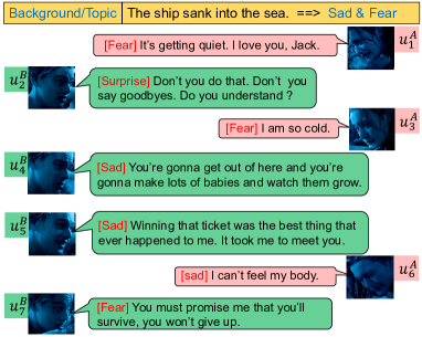
Figure 1: Emotions are affected by multiple uni-modal, global contextual, intra- and inter-person dependencies. Images are from the movie “Titanic”.

Figure 1 shows that emotions expressed in a dialogue are affected by three main factors: 1) multiple uni-modalities (different modalities complete each other to provide a more informative utterance representation); 2) global contextual information ($u_{3}^{A}$ depends on the topic “The ship sank into the sea”, indicating fear); and 3) intra-person and inter-person dependencies ($u_{6}^{A}$ becomes sad affected by sadness in $u_{4}^{B}\&u_{5}^{B}$). Depending on how to model intra-person and inter-person dependencies, current MERC methods can be categorized into Sequence-based and Graph-based methods. The former (Dai et al., 2021; Mao et al., 2022; Liang et al., 2022) use recurrent neural networks or Transformers to model the temporal interaction between utterances. However, they failed to distinguish intra-speaker and inter-speaker dependencies and easily lost uni-modal specific features by the cross-modal attention mechanism (Rajan et al., 2022). Graph structure (Joshi et al., 2022; Wei et al., 2019) solves these issues by using edges between nodes (speakers) to distinguish intra-speaker and inter-speaker dependencies. Graph Neural Networks (GNNs) further help nodes learn common features by aggregating information from neighbours while maintaining their uni-modal specific features.

Although graph-based MERC methods have achieved great success, there still remain problems that need to be solved: 1) Current methods directly aggregate features of multiple modalities (Joshi et al., 2022) or project modalities into a latent space to learn representations (Li et al., 2022e), which ignores the diversity of each modality and fails to capture richer semantic information from each modality. They also ignore global contextual information during the feature fusion process, leading to poor performance. 2) Since all graph-based methods adopt GNN (Scarselli et al., 2009) or Graph Convolutional Networks (GCNs) (Kipf and Welling, 2017), with the number of layers deepening, the phenomenon of over-smoothing starts to appear, resulting in the representation of similar sentiments being indistinguishable. 3) Most methods use a two-phase pipeline (Fu et al., 2021; Joshi et al., 2022), where they first extract and fuse uni-modal features as utterance representations and then fix them as input for graph models. However, the two-phase pipeline will lead to sub-optimal performance since the fused representations are fixed and cannot be further improved to benefit from the downstream supervisory signals.

To solve the above-mentioned problems, we propose Joint multimodality fusion and graph contrastive learning for MERC (Joyful), where multimodality fusion, graph contrastive learning (GCL), and multimodal emotion recognition are jointly optimized in an overall objective function. 1) We first design a new multimodal fusion mechanism that can simultaneously learn and fuse a global contextual representation and uni-modal specific representations. For the global contextual representation, we smooth it with a proposed topic-related vector to maintain its consistency, where the topic-related vector is temporally updated since the topic usually changes. For uni-modal specific representations, we project them into a shared subspace to fully explore their richer semantics without losing alignment with other modalities. 2) To alleviate the over-smoothing issue of deeper GNN layers, inspired by You et al. (2020), that showed contrastive learning could provide more distinguishable node representations to benefit various downstream tasks, we propose a cross-view GCL-based framework to alleviate the difficulty of categorizing similar emotions, which helps to learn more distinctive utterance representations by making samples with the same sentiment cohesive and those with different sentiments mutually exclusive. Furthermore, graph augmentation strategies are designed to improve Joyful’s robustness and generalizability. 3) We jointly optimize each part of Joyful in an end-to-end manner to ensure global optimized performance. The main contributions of this study can be summarized as follows:

•  We propose a novel joint leaning framework for MERC, where multimodality fusion, GCL, and emotion recognition are jointly optimized for global optimal performance. Our new multimodal fusion mechanism can obtain better representations by simultaneously depicting global contextual and local uni-modal specific features.

•  To the best of our knowledge, Joyful is the first method to utilize graph contrastive learning for MERC, which significantly improves the model’s ability to distinguish different sentiments. Multiple graph augmentation strategies further improve the model’s stability and generalization.

•  Extensive experiments conducted on three multimodal benchmark datasets demonstrated the effectiveness and robustness of Joyful.

2 Related Work

2.1 Multimodal Emotion Recognition

Depending on how to model the context of utterances, existing MERC methods are categorized into three classes: Recurrent-based methods (Majumder et al., 2019; Mao et al., 2022) adopt RNN or LSTM to model the sequential context for each utterance. Transformers-based methods (Ling et al., 2022; Liang et al., 2022; Le et al., 2022) use Transformers with cross-modal attention to model the intra- and inter-speaker dependencies. Graph-based methods Joshi et al. (2022); Zhang et al. (2021); Fu et al. (2021) can control context information for each utterance and provide accurate intra- and inter-speaker dependencies, achieving SOTA performance on many MERC benchmark datasets.

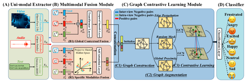
Figure 2: Overview of Joyful. We first extract uni-modal features, fuse them using a multimodal fusion module, and use them as input of the GCL-based framework to learn better representations for emotion recognition.

2.2 Multimodal Fusion Mechanism

Learning effective fusion mechanisms is one of the core challenges in multimodal learning (Shankar, 2022). By capturing the interactions between different modalities more reasonably, deep models can acquire more comprehensive information. Current fusion methods can be classified into aggregation-based (Wu et al., 2021; Guo et al., 2021), alignment-based (Liu et al., 2020; Li et al., 2022e), and their mixture (Wei et al., 2019; Nagrani et al., 2021). Aggregation-based fusion methods (Zadeh et al., 2017; Chen et al., 2021) adopt concatenation, tensor fusion and memory fusion to combine multiple modalities. Alignment-based fusion centers on latent cross-modal adaptation, which adapts streams from one modality to another (Wang et al., 2022a). Different from the above methods, we learn global contextual information by concatenation while fully exploring the specific patterns of each modality in an alignment manner.

2.3 Graph Contrastive Learning

GCL aims to learn representations by maximizing feature consistency under differently augmented views, that exploit data- or task-specific augmentations, to inject the desired feature invariance You et al. (2020). GCL has been well used in the NLP community via self-supervised and supervised settings. Self-supervised GCL first creates augmented graphs by edge/node deletion and insertion (Zeng and Xie, 2021), or attribute masking (Zhang et al., 2022). It then captures the intrinsic patterns and properties in the augmented graphs without using human provided labels. Supervised GCL designs adversarial (Sun et al., 2022) or geometric (Li et al., 2022d) contrastive loss to make full use of label information. For example, Li et al. (2022c) first used supervised CL for emotion recognition, greatly improving the performance. Inspired by previous studies, we jointly consider self-supervised (suitable graph augmentation) and supervised (cross-entropy) manners to fully explore graph structural information and downstream supervisory signals.

3 Methodology

Figure 2 shows an overview of Joyful, which mainly consists of four components: (A) a uni-modal extractor, (B) a multimodal fusion (MF) module, (C) a graph contrastive learning module, and (D) a classifier. Hereafter, we give formal notations and the task definition of Joyful, and introduce each component subsequently in detail.

3.1 Notations and Task Definition

In dialogue emotion recognition, a training dataset $\mathcal{D}=\{(\mathcal{C}_{i},\mathcal{Y}_{i})\}_{i=1}^{N}$ is given, where $\mathcal{C}_{i}$ represents the $i$-th conversation, each conversation contains several utterances $\mathcal{C}_{i}=\{\bm{u}_{1},\dots,\bm{u}_{m}\}$, and $\mathcal{Y}_{i}\in\mathbf{Y}^{m}$, given label set $\mathbf{Y}=\{y_{1},\dots,y_{k}\}$ of $k$ emotion classes. Let $\mathbf{X}^{v}$, $\mathbf{X}^{a}$, $\mathbf{X}^{t}$ be the visual, audio, and text feature spaces, respectively. The goal of MERC is to learn a function $\mathbf{F}:\mathbf{X}^{v}\times\mathbf{X}^{a}\times\mathbf{X}^{t}\to\mathbf{Y}$ that can recognize the emotion label for each utterance. We utilize three widely used multimodal conversational benchmark datasets, namely IEMOCAP, MOSEI, and MELD, to evaluate the performance of our model. Please see Section 4.1 for their detailed statistical information.

3.2 Uni-modal Extractor

For IEMOCAP (Busso et al., 2008), video features $\bm{x}_{v}$ $\in$ $\mathbb{R}^{512}$, audio features $\bm{x}_{a}\in\mathbb{R}^{100}$, and text features $\bm{x}_{t}\in\mathbb{R}^{768}$ are obtained from OpenFace (Baltrusaitis et al., 2018), OpenSmile (Eyben et al., 2010) and SBERT (Reimers and Gurevych, 2019), respectively. For MELD (Poria et al., 2019a), $\bm{x}_{v}\in\mathbb{R}^{342}$, $\bm{x}_{a}\in\mathbb{R}^{300}$, and $\bm{x}_{t}\in\mathbb{R}^{768}$ are obtained from DenseNet (Huang et al., 2017), OpenSmile, and TextCNN (Kim, 2014). For MOSEI (Zadeh et al., 2018), $\bm{x}_{v}\in\mathbb{R}^{35}$, $\bm{x}_{a}\in\mathbb{R}^{80}$, and $\bm{x}_{t}\in\mathbb{R}^{768}$ are obtained from TBJE (Delbrouck et al., 2020), LibROSA (Raguraman et al., 2019), and SBERT. Textual features are sentence-level static features. Audio and visual modalities are utterance-level features by averaging all the token features.

3.3 Multimodal Fusion Module

Though the uni-modal extractors can capture long-term temporal context, they are unable to handle feature redundancy and noise due to the modality gap. Thus, we design a new multimodal fusion module (Figure 2 (B)) to inherently separate multiple modalities into two disjoint parts, contextual representations and specific representations, to extract the consistency and specificity of heterogeneous modalities collaboratively and individually.

3.3.1 Contextual Representation Learning

Contextual representation learning aims to explore and learn hidden contextual intent/topic knowledge of the dialogue, which can greatly improve the performance of Joyful. In Figure 2 (B1), we first project all uni-modal inputs $\bm{x}_{\{v,a,t\}}$ into a latent space by using three separate connected deep neural networks $f_{\{v,a,t\}}^{g}(\cdot)$ to obtain hidden representations $\bm{z}_{\{v,a,t\}}^{g}$. Then, we concatenate them as $\bm{z}_{m}^{g}$ and apply it to a multi-layer transformer to maximize the correlation between multimodal features, where we learn a global contextual multimodal representation $\hat{\bm{z}}_{m}^{g}$. Considering that the contextual information will change over time, we design a temporal smoothing strategy for $\hat{\bm{z}}_{m}^{g}$ as

$$\mathcal{J}_{smooth}=\|\hat{\bm{z}}_{m}^{g}-\bm{z}_{con}\|^{2},$$ (1)

where $\bm{z}_{con}$ is the topic-related vector describing the high-level global contextual information without requiring topic-related inputs, following the definition in Joshi et al. (2022). We update the ($i$+1)-th utterance as $\bm{z}_{con}\leftarrow\bm{z}_{con}+e^{\eta*i}\hat{\bm{z}}_{m}^{g}$, and $\eta$ is the exponential smoothing parameter (Shazeer and Stern, 2018), indicating that more recent information will be more important.

To ensure fused contextual representations capture enough details from hidden layers, Hazarika et al. (2020) minimized the reconstruction error between fused representations with hidden representations. Inspired by their work, to ensure that $\hat{\bm{z}}_{m}^{g}$ contains essential modality cues for downstream emotion recognition, we reconstruct $\bm{z}_{m}^{g}$ from $\hat{\bm{z}}_{m}^{g}$ by minimizing their Euclidean distance:

$$\mathcal{J}_{rec}^{g}=\|\hat{\bm{z}}_{m}^{g}-\bm{z}_{m}^{g}\|^{2}.$$ (2)

3.3.2 Specific Representation Learning

Specific representation learning aims to fully explore specific information from each modality to complement one another. Figure 2 (B2) shows that we first use three fully connected deep neural networks $f_{\{v,a,t\}}^{\ell}(\cdot)$ to project uni-modal embeddings $\bm{x}_{\{v,a,t\}}$ into a hidden space with representations as $\bm{z}_{\{v,a,t\}}^{\ell}$. Considering that visual, audio, and text features are extracted with different encoding methods, directly applying multiple specific features as an input for the downstream emotion recognition task will degrade the model’s accuracy. To solve it, the multimodal features are projected into a shared subspace, and a shared trainable basis matrix is designed to learn aligned representations for them. Therefore, the multimodal features can be fully integrated and interacted to mitigate feature discontinuity and remove noise across modalities. We define a shared trainable basis matrix $\mathbf{B}$ with $q$ basis vectors as $\mathbf{B}=(\bm{b}_{1},\dots,\bm{b}_{q})^{T}\in\mathbb{R}^{q\times d_{b}}$ with $d_{b}$ representing the dimensionality of each basis vector. Here, $T$ indicates transposition. Then, $\bm{z}_{\{v,a,t\}}^{\ell}$ and $\mathbf{B}$ are projected into the shared subspace:

$$\tilde{\bm{z}}_{\{v,a,t\}}^{\ell}=\mathbf{W}_{\{v,a,t\}}\bm{z}_{\{v,a,t\}}^{\ell},\,\,\,\,\,\widetilde{\mathbf{B}}=\mathbf{B}\mathbf{W}_{b},$$ (3)

where $\mathbf{W}_{\{v,a,t,b\}}$ are trainable parameters. To learn new representations for each modality, we calculate the cosine similarity between them and $\mathbf{B}$ as

$$S_{ij}^{\{v,a,t\}}=(\tilde{\bm{z}}_{\{v,a,t\}}^{\ell})_{i}\cdot\widetilde{\bm{b}}_{j},$$ (4)

where $S_{ij}^{v}$ denotes the similarity between the $i$-th visual feature $(\tilde{\bm{z}}_{v}^{\ell})_{i}$ and the $j$-th basis vector representation $\widetilde{\bm{b}}_{j}$. To prevent inaccurate representation learning caused by an excessive weight of a certain item, the similarities are further normalized by

$$S_{ij}^{\{v,a,t\}}=\frac{\exp{(S_{ij}^{\{v,a,t\}})}}{\sum_{k=1}^{q}\exp{(S_{ik}^{\{v,a,t\}})}}.$$ (5)

Then, the new representations are obtained as

$$(\hat{\bm{z}}_{\{v,a,t\}}^{\ell})_{i}=\sum_{k=1}^{q}S_{ik}^{\{v,a,t\}}\cdot\widetilde{\bm{b}}_{k},$$ (6)

where $\hat{\bm{z}}_{\{v,a,t\}}^{\ell}$ are new representations, and we also use reconstruction loss for their combinations

$$\mathcal{J}_{rec}^{\ell}=\|\hat{\bm{z}}_{m}^{\ell}-\bm{z}_{m}^{\ell}\|^{2},$$ (7)

where Concat( , ) indicating the concatenation, i.e., $\hat{\bm{z}}_{m}^{\ell}$=$\textit{Concat}(\hat{\bm{z}}_{v}^{\ell},\hat{\bm{z}}_{a}^{\ell},\hat{\bm{z}}_{t}^{\ell})$, $\bm{z}_{m}^{\ell}$ = $\textit{Concat}(\bm{z}_{v}^{\ell},\bm{z}_{a}^{\ell},\bm{z}_{t}^{\ell})$.

Finally, we define the multimodal fusion loss by combining Eqs.(1), (2), and (7) as:

$$\mathcal{L}_{mf}=\mathcal{J}_{smooth}+\mathcal{J}_{rec}^{g}+\mathcal{J}_{rec}^{\ell}.$$ (8)

3.4 Graph Contrastive Learning Module

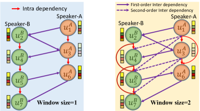
Figure 3: An example of graph construction.

3.4.1 Graph Construction

Graph construction aims to establish relations between past and future utterances that preserve both intra- and inter-speaker dependencies in a dialogue. We define the $i$-th dialogue with $P$ speakers as $\mathcal{C}_{i}$ = $\{\mathcal{U}^{S_{1}},\dots,\mathcal{U}^{S_{P}}\}$, where $\mathcal{U}^{S_{i}}$ = $\{\bm{u}_{1}^{S_{i}},\dots,\bm{u}_{m}^{S_{i}}\}$ represents the set of utterances spoken by speaker $S_{i}$. Following Ghosal et al. (2019), we define a graph with nodes representing utterances and directed edges representing their relations: $\mathcal{R}_{ij}=\bm{u}_{i}\to\bm{u}_{j}$, where the arrow represents the speaking order. Intra-Dependency ($\mathcal{R}_{intra}\in\{\mathcal{U}^{S_{i}}\to\mathcal{U}^{S_{i}}\}$) represents intra-relations between the utterances (red lines), and Inter-Dependency ($\mathcal{R}_{inter}\in\{\mathcal{U}^{S_{i}}\to\mathcal{U}^{S_{j}}\},i\neq j$) represents the inter-relations between the utterances (purple lines), as shown in Figure 3. All nodes are initialized by concatenating contextual and specific representations as $\bm{h}_{m}$ = Concat($\hat{\bm{z}}_{m}^{g},\hat{\bm{z}}_{m}^{\ell}$). And we show that window size is a hyper-parameter that controls the context information for each utterance and provide accurate intra- and inter-speaker dependencies.

3.4.2 Graph Augmentation

Graph Augmentation (GA): Inspired by Zhu et al. (2020), creating two augmented views by using different ways to corrupt the original graph can provide highly heterogeneous contexts for nodes. By maximizing the mutual information between two augmented views, we can improve the robustness of the model and obtain distinguishable node representations (You et al., 2020). However, there are no universally appropriate GA methods for various downstream tasks (Xu et al., 2021), which motivates us to design specific GA strategies for MERC. Considering that MERC is sensitive to initialized representations of utterances, intra-speaker and inter-speaker dependencies, we design three corresponding GA methods:

• Feature Masking (FM): given the initialized representations of utterances, we randomly select $p$ dimensions of the initialized representations and mask their elements with zero, which is expected to enhance the robustness of Joyful to multimodal feature variations;

• Edge Perturbation (EP): given the graph $\mathcal{G}$, we randomly drop and add $p\%$ of intra- and inter-speaker edges, which is expected to enhance the robustness of Joyful to local structural variations;

• Global Proximity (GP): given the graph $\mathcal{G}$, we first use the Katz index (Katz, 1953) to calculate high-order similarity between intra- and inter-speakers, and randomly add $p\%$ high-order edges between speakers, which is expected to enhance the robustness of Joyful to global structural variations (Examples in Appendix A).

We propose a hybrid scheme for generating graph views on both structure and attribute levels to provide diverse node contexts for the contrastive objective. Figure 2 (C) shows that the combination of (FM $\&$ EP) and (FM $\&$ GP) are adopted to obtain two correlated views.

3.4.3 Graph Contrastive Learning

Graph contrastive learning adopts an $L$-th layer GCNs as a graph encoder to extract node hidden representations $\mathbf{H}^{(1)}$ = {$\bm{h}^{(1)}_{1}$, $\dots$, $\bm{h}^{(1)}_{m}$} and $\mathbf{H}^{(2)}$ = {$\bm{h}^{(2)}_{1}$, $\dots$, $\bm{h}^{(2)}_{m}$} for two augmented graphs, where $\bm{h}_{i}$ is the hidden representation for the $i$-th node. We follow an iterative neighborhood aggregation (or message passing) scheme to capture the structural information within the nodes’ neighborhood. Formally, the propagation and aggregation of the $\ell$-th GCN layer is:

$$\bm{a}_{(i,\,\ell)}= \,\,\,\textrm{AGG}_{(\ell)\,}(\{\bm{h}_{(j,\,\ell-1)}|j\in\mathbf{N}_{i}\})$$ (9)

$$\bm{h}_{(i,\,\ell)}= \,\,\,\textrm{COM}_{(\ell)\,}(\bm{h}_{(i,\,\ell-1)}\oplus\bm{a}_{(i,\,\ell)}),$$ (10)

where $\bm{h}_{(i,\,\ell)}$ is the embedding of the $i$-th node at the $\ell$-th layer, $\bm{h}_{(i,\,0)}$ is the initialization of the $i$-th utterance, $\mathbf{N}_{i}$ represents all neighbour nodes of the $i$-th node, and $\text{AGG}_{(\ell)}(\cdot)$ and $\text{COM}_{(\ell)}(\cdot)$ are aggregation and combination of the $\ell$-th GCN layer (Hamilton et al., 2017). For convenience, we define $\bm{h}_{i}=\bm{h}_{(i,L)}$. After the $L$-th GCN layer, final node representations of two views are $\mathbf{H}^{(1)}$ / $\mathbf{H}^{(2)}$.

In Figure 2 (C3), we design the intra- and inter-view graph contrastive losses to learn distinctive node representations. We start with the inter-view contrastiveness, which pulls closer the representations of the same nodes in two augmented views while pushing other nodes away, as depicted by the red and blue dash lines in Figure 2 (C3). Given the definition of our positive and negative pairs as $(\bm{h}_{i}^{(1)},\bm{h}_{i}^{(2)})^{+}$ and $(\bm{h}_{i}^{(1)},\bm{h}_{j}^{(2)})^{-}$, where $i\neq j$, the inter-view loss for the $i$-th node is formulated as:

$$\mathcal{L}_{inter}^{i}=-\log\frac{\exp(\text{sim}(\bm{h}_{i}^{(1)},\bm{h}_{i}^{(2)}))}{\sum\limits_{j=1}^{m}\exp(\text{sim}(\bm{h}_{i}^{(1)},\bm{h}_{j}^{(2)}))},$$ (11)

where $\text{sim}(\cdot,\cdot)$ denotes the similarity between two vectors, i.e., the cosine similarity in this paper.

Intra-view contrastiveness regards all nodes except the anchor node as negatives within a particular view (green dash lines in Figure 2 (C3)), as defined $(\bm{h}_{i}^{(1)},\bm{h}_{j}^{(1)})^{-}$ where $i\neq j$. The intra-view contrastive loss for the $i$-th node is defined as:

$$\mathcal{L}_{intra}^{i}=-\log\frac{\exp(\text{sim}(\bm{h}_{i}^{(1)},\bm{h}_{i}^{(2)}))}{\sum\limits_{j=1}^{m}\exp(\text{sim}(\bm{h}_{i}^{(1)},\bm{h}_{j}^{(1)}))}.$$ (12)

By combining the inter- and intra-view contrastive losses of Eqs.(11) and (12), the contrastive objective function $\mathcal{L}_{ct}$ is formulated as:

$$\mathcal{L}_{ct}=\frac{1}{2m}\sum\limits_{i=1}^{m}(\mathcal{L}_{inter}^{i}+\mathcal{L}_{intra}^{i}).$$ (13)

3.5 Emotion Recognition Classifier

We use cross-entropy loss for classification as:

$$\mathcal{L}_{ce}=-\frac{1}{m}\sum_{i=1}^{m}\sum_{j=1}^{k}y^{j}_{i}\log{(\hat{y}_{i}^{j})},$$ (14)

where $k$ is the number of emotion classes, $m$ is the number of utterances, $\hat{y}_{i}^{j}$ is the $i$-th predicted label, and $y_{i}^{j}$ is the $i$-th ground truth of $j$-th class.

Above all, combining the MF loss of Eq.(8), contrastive loss of Eq.(13), and classification loss of Eq.(14) together, the final objective function is

$$\mathcal{L}_{all}=\bm{\alpha}\mathcal{L}_{mf}+\bm{\beta}\mathcal{L}_{ct}+\mathcal{L}_{ce},$$ (15)

where $\bm{\alpha}$ and $\bm{\beta}$ are the trade-off hyper-parameters. We give our pseudo-code in Appendix F.

Dataset	Train	Valid	Test
IEMOCAP(4-way)	3,200/108	400/12	943/31
IEMOCAP(6-way)	5,146/108	664/12	1,623/31
MELD	9,989/1,039	1,109/114	2,80/2,610
MOSEI	16,327/2,249	1,871/300	4,662/679

Table 1: Utterances/Conversations of four datasets.

4 Experiments and Result Analysis

4.1 Experimental Settings

Datasets and Metrics. In Table 1, IEMOCAP is a conversational dataset where each utterance was labeled with one of the six emotion categories (Anger, Excited, Sadness, Happiness, Frustrated and Neutral). Following COGMEN, two IEMOCAP settings were used for testing, one with four emotions (Anger, Sadness, Happiness and Neutral) and one with all six emotions, where 4-way directly removes the additional two emotion labels (Excited and Frustrated). MOSEI was labeled with six emotion labels (Anger, Disgust, Fear, Happiness, Sadness, and Surprise). For six emotion labels, we conducted two settings: binary classification considers the target emotion as one class and all other emotions as another class, and multi-label classification tags multiple labels for each utterance. MELD was labeled with six universal emotions (Joy, Sadness, Fear, Anger, Surprise, and Disgust). We split the datasets into 70%/10%/20% as training/validation/test data, respectively. Following Joshi et al. (2022), we used Accuracy and Weighted F1-score (WF1) as evaluation metrics. Please note that the detailed label distribution of the datasets is given in Appendix I.

Implementation Details. We selected the augmentation pairs (FM & EP) and (FM & GP) for two views. We set the augmentation ratio $p$=20% and smoothing parameter $\eta$=0.2, and applied the Adam (Kingma and Ba, 2015) optimizer with an initial learning rate of 3$e$-5. For a fair comparison, we followed the default parameter settings of the baselines and repeated all experiments ten times to report the average accuracy. We conducted the significance by t-test with Benjamini-Hochberg (Benjamini and Hochberg, 1995) correction (Please see details in Appendix G).

Baselines. Different MERC datasets have different best system results, following COGMEN, we selected SOTA baselines for each dataset. For IEMOCAP-4, we selected Mult (Tsai et al., 2019a), RAVEN (Wang et al., 2019), MTAG (Yang et al., 2021), PMR (Lv et al., 2021), COGMEN and MICA (Liang et al., 2021) as our baselines. For IEMOCAP-6, we selected Mult, FE2E Dai et al. (2021), DiaRNN Majumder et al. (2019), COSMIC (Ghosal et al., 2020), Af-CAN (Wang et al., 2021), AGHMN (Jiao et al., 2020), COGMEN and RGAT (Ishiwatari et al., 2020) as our baselines. For MELD, we selected DiaGCN (Ghosal et al., 2019), DiaCRN (Hu et al., 2021), MMGCN (Wei et al., 2019), UniMSE (Hu et al., 2022b), COGMEN and MM-DFN (Hu et al., 2022a) as baselines. For MOSEI, we selected Mul-Net (Shenoy et al., 2020), TBJE (Delbrouck et al., 2020), COGMEN and MR (Tsai et al., 2020).

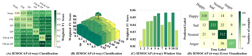
Figure 4: (A) WF1 gain with different augmentation pairs; (B$\sim$C) Parameter tuning; (D) Imbalanced dataset.

4.2 Parameter Sensitive Study

We first examined whether applying different data augmentation methods improves Joyful. We observed in Figure 4 (A) that 1) all data augmentation strategies are effective 2) applying augmentation pairs of the same type cannot result in the best performance; and 3) applying augmentation pairs of different types improves performance. Thus, we selected (FM $\&$ EP) and (FM $\&$ GP) as the default augmentation strategy since they achieved the best performance (More details please see Appendix C).

Joyful has three hyperparameters. $\bm{\alpha}$ and $\bm{\beta}$ determine the importance of MF and GCL in Eq.(15), and window size controls the contextual length of conversations. In Figure 4 (B), we observed how $\bm{\alpha}$ and $\bm{\beta}$ affect the performance of Joyful by varying $\bm{\alpha}$ from 0.02 to 0.10 in 0.02 intervals and $\bm{\beta}$ from 0.1 to 0.5 in 0.1 intervals. The results indicated that Joyful achieved the best performance when $\bm{\alpha}\in\left[0.06,0.08\right]$ and $\bm{\beta}$ = 0.3. Figure 4 (C) shows that when ${window\_size}$ = 8, Joyful achieved the best performance. A small window size will miss much contextual information, and a longer one contains too much noise, we set it as 8 in experiments (Details in Appendix D).

Method	IEMOCAP 6-way (F1) $\,\uparrow$						Average $\,\uparrow$
	Hap.	Sad.	Neu.	Ang.	Exc.	Fru.	Acc.	WF1
Mult	48.23	76.54	52.38	60.04	54.71	57.51	58.04	58.10
FE2E	44.82	64.98	56.09	62.12	61.02	57.14	58.30	57.69
DiaRNN	32.88	78.08	59.11	63.38	73.66	59.41	63.34	62.85
COSMIC	53.23	78.43	62.08	65.87	69.60	61.39	64.88	65.38
Af-CAN	37.01	72.13	60.72	67.34	66.51	66.13	64.62	63.74
AGHMN	52.10	73.30	58.40	61.91	69.72	62.31	63.58	63.54
RGAT	51.62	77.32	65.42	63.01	67.95	61.23	65.55	65.22
COGMEN	51.91	81.72	68.61	66.02	75.31	58.23	68.26	67.63
Joyful	$\textbf{\,\,\,60.94}^{{\dagger}}$	$\textbf{\,\,\,84.42}^{{\dagger}}$	68.24	$\textbf{\,\,\,69.95}^{{\dagger}}$	73.54	$\textbf{\,\,\,67.55}^{{\dagger}}$	$\textbf{\,\,\,70.55}^{{\dagger}}$	$\textbf{\,\,\,71.03}^{{\dagger}}$

Table 2: Overall performance comparison on IEMOCAP (6-way) in the multimodal (A+T+V) setting. Symbol ${\dagger}$ indicates that Joyful significantly surpassed all baselines using t-test with $p<0.005$.

Method	Happy	Sadness	Neutral	Anger	WF1
Mult	88.4	86.3	70.5	87.3	80.4
RAVEN	86.2	83.2	69.4	86.5	78.6
MTAG	85.9	80.1	64.2	76.8	73.9
PMR	89.2	87.1	71.3	87.3	81.0
MICA	83.7	75.5	61.8	72.6	70.7
COGMEN	78.8	86.8	84.6	88.0	84.9
Joyful	80.1	$\textbf{\,\,\,\,88.1}^{{\dagger}}$	$\textbf{\,\,\,85.1}^{{\dagger}}$	$\textbf{\,\,\,\,88.1}^{{\dagger}}$	$\textbf{\,\,\,\,85.7}^{{\dagger}}$

Table 3: Overall performance comparison on IEMOCAP (4-way) in the multimodal (A+T+V) setting.

4.3 Performance of Joyful

Tables 2 & 3 show that Joyful outperformed all baselines in terms of accuracy and WF1, improving 5.0% and 1.3% in WF1 for 6-way and 4-way, respectively. Graph-based methods, COGMEN and Joyful, outperform Transformers-based methods, Mult and FE2E. Transformers-based methods cannot distinguish intra- and inter-speaker dependencies, distracting their attention to important utterances. Furthermore, they use the cross-modal attention layer, which can enhance common features among modalities while losing uni-modal specific features (Rajan et al., 2022). Joyful outperforms other GNN-based methods since it explored features from both the contextual and specific levels, and used GCL to obtain more distinguishable features. However, Joyful cannot improve in Happy for 4-way and in Excited for 6-way since samples in IEMOCAP were insufficient for distinguishing these similar emotions (Happy is 1/3 of Neutral in Fig. 4 (D)). Without labels’ guidance to re-sample or re-weight the underrepresented samples, self-supervised GCL, utilized in Joyful, cannot ensure distinguishable representations for samples of minor classes by only exploring graph topological information and vertex attributes.

Methods	Emotion Categories of MELD (F1) $\uparrow$					Average $\uparrow$
	Neu.	Sur.	Sad.	Joy	Anger	Acc.	WF1
DiaGCN	75.97	46.05	19.60	51.20	40.83	58.62	56.36
DiaCRN	77.01	50.10	26.63	52.77	45.15	61.11	58.67
MMGCN	76.33	48.15	26.74	53.02	46.09	60.42	58.31
UniMSE	74.61	48.21	31.15	54.04	45.26	59.39	58.19
COGMEN	75.31	46.75	33.52	54.98	45.81	58.35	58.66
MM-DFN	77.76	50.69	22.93	54.78	47.82	62.49	59.46
Joyful	76.80	$\textbf{\,\,\,51.91}^{{\dagger}}$	$\textbf{\,\,\,41.78}^{{\dagger}}$	$\textbf{\,\,\,56.89}^{{\dagger}}$	$\textbf{\,\,\,50.71}^{{\dagger}}$	$\textbf{\,\,\,62.53}^{{\dagger}}$	$\textbf{\,\,\,61.77}^{{\dagger}}$

Table 4: Results on MELD with the multimodal setting. Underline indicates our reproduced results.

Method	Happy	Sadness	Anger	Fear	Disgust	Surprise
	Binary Classification (F1)$\,\uparrow$
Mul-Net	67.9	65.5	67.2	87.6	74.7	86.0
TBJE	63.8	68.0	74.9	84.1	83.8	86.1
MR	65.9	66.7	71.0	85.9	80.4	85.9
COGMEN	70.4	72.3	76.2	88.1	83.7	85.3
Joyful	$\textbf{\,\,\,\,71.7}^{{\dagger}}$	$\textbf{\,73.4}^{{\dagger}}$	$\textbf{\,78.9}^{{\dagger}}$	88.2	$\textbf{\,85.1}^{{\dagger}}$	86.1
	Multi-label Classification (F1)$\,\uparrow$
Mul-Net	70.8	70.9	74.5	86.2	83.6	87.7
TBJE	68.4	73.9	74.4	86.3	83.1	86.6
MR	69.6	72.2	72.8	86.5	82.5	87.9
COGMEN	72.7	73.9	78.0	86.7	85.5	88.3
Joyful	70.9	$\textbf{\,74.6}^{{\dagger}}$	$\textbf{\,78.1}^{{\dagger}}$	$\textbf{\,89.4}^{{\dagger}}$	$\textbf{\,86.8}^{{\dagger}}$	$\textbf{\,90.5}^{{\dagger}}$

Table 5: Results on MOSEI with the multimodal setting.

Tables 4 & 5 show that Joyful outperformed the baselines in more complex scenes with multiple speakers or various emotional labels. Compared with COGMEN and MM-DFN, which directly aggregate multimodal features, Joyful can fully explore features from each uni-modality by specific representation learning to improve the performance. The GCL module can better aggregate similar emotional features for utterances to obtain better performance for multi-label classification. We cannot improve in Happy on MOSEI since the samples are imbalanced and Happy has only 1/6 of Surprise, making Joyful hard to identify it.

Modality	IEMOCAP-4		IEMOCAP-6		MOSEI (WF1)
	Acc.	WF1	Acc.	WF1	Binary	Multi-label
Audio	64.8	63.3	49.2	48.0	51.2	53.3
Text	83.0	83.0	67.4	67.5	73.6	73.9
Video	44.6	43.4	28.2	28.6	23.6	24.4
A+T	82.6	82.5	67.5	67.8	74.7	74.9
A+V	68.0	67.5	52.7	52.5	61.7	62.4
T+V	80.0	80.0	65.2	65.5	73.1	73.4
w/o MF(B1)	85.3	85.4	70.0	70.3	76.2	76.5
w/o MF(B2)	85.2	85.1	69.2	69.5	75.8	76.2
w/o MF	85.2	84.9	69.0	69.2	75.4	75.8
COGMEN w/o GNN	80.1	80.2	62.7	62.9	72.3	72.9
w/o GCL	84.7	84.7	66.1	66.5	73.8	73.4
Joyful	$\textbf{\,\,85.6}^{{\dagger}}$	$\textbf{\,\,85.7}^{{\dagger}}$	$\textbf{\,\,\,70.5}^{{\dagger}}$	$\textbf{\,\,\,71.0}^{{\dagger}}$	$\textbf{\,\,\,76.9}^{{\dagger}}$	$\textbf{\,\,77.2}^{{\dagger}}$

Table 6: Ablation study with different modalities.

To verify the performance gain from each component, we conducted additional ablation studies. Table 6 shows multi-modalities can greatly improve Joyful’s performance compared with each single modality. GCL and each component of MF can separately improve the performance of Joyful, showing their effectiveness (Visualization in Appendix H). Joyful w/o GCL and COGMEN w/o GNN utilize only a multimodal fusion mechanism for classification without additional modules for optimizing node representations. The comparison between them demonstrates the effectiveness of the multimodal fusion mechanism in Joyful.

Method	One-Layer (WF1)		Two-Layer (WF1)		Four-Layer (WF1)
	COGMEN	Joyful	COGMEN	Joyful	COGMEN	Joyful
Unattack	67.63	71.03	63.21	71.05	58.39	70.96
5% Noisy	65.26	70.82	61.35	70.55	56.28	70.10
10% Noisy	62.26	70.33	59.24	70.45	53.21	69.23
15% Noisy	57.28	69.98	55.18	69.21	52.32	67.96
20% Noisy	54.22	68.52	51.79	68.82	50.72	67.23

Table 7: Adversarial attacks for GNN with different depth on 6-way IEMOCAP.

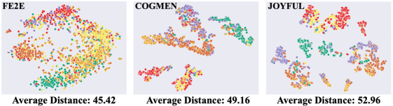
Figure 5: t-SNE visualization of IEMOCAP (6-way).

We deepened the GNN layers to verify Joyful’s ability to alleviate the over-smoothing. In Table 7, COGMEN with four-layer GNN was 9.24% lower than that with one-layer, demonstrating that the over-smoothing decreases performance, while Joyful relieved this issue by using the GCL framework. To verify the robustness, following Tan et al. (2022), we randomly added 5%$\sim$20% noisy edges to the training data. In Table 7, COGMEN was easily affected by the noise, decreasing 10.8% performance in average with 20% noisy edges, while Joyful had strong robustness with only an average 2.8% performance reduction for 20% noisy edges.

To show the distinguishability of the node representations, we visualize the node representations of FE2E, COGMEN, and Joyful on 6-way IEMOCAP. In Figure 5, COGMEN and Joyful obtained more distinguishable node representations than FE2E, demonstrating that graph structure is more suitable for MERC than Transformers. Joyful performed better than COGMEN, illustrating the effectiveness of GCL. In Figure 6, we randomly sampled one example from each emotion of IEMOCAP (6-way) and chose best-performing COGMEN for comparison. Joyful obtained more discriminate prediction scores among emotion classes, showing GCL can push samples from different emotion class farther apart.

Figure 6: Visualization of emotion probability, each first row is Joyful and each second row is COGMEN.

5 Conclusion

We proposed a joint learning model (Joyful) for MERC, that involves a new multimodal fusion mechanism and GCL module to effectively improve the performance of MERC. The MR mechanism can extract and fuse contextual and uni-modal specific emotion features, and the GCL module can help learn more distinguishable representations. For future work, we plan to investigate the performance of using supervised GCL for Joyful on unbalanced and small-scale emotional datasets.

Limitations

Joyful has a limited ability to classify minority classes with fewer samples in unbalanced datasets. Although we utilized self-supervised graph contrastive learning to learn a distinguishable representation for each utterance by exploring vertex attributes, graph structure, and contextual information, GCL failed to separate classes with fewer samples from the ones with more samples because the utilized self-supervised learning lacks the label information and does not balance the label distribution. Another limitation of Joyful is that its framework was designed specifically for multimodal emotion recognition tasks, which is not straightforward and general as language models (Devlin et al., 2019; Liu et al., 2019) or image processing techniques (LeCun et al., 1995). This setting may limit the applications of Joyful for other multimodal tasks, such as the multimodal sentiment analysis task (Detailed experiments in Appendix J) and the multimodal retrieval task. Finally, although Joyful achieved SOTA performances on three widely-used MERC benchmark datasets, its performance on larger-scale and more heterogeneous data in real-world scenarios is still unclear.

Appendix A Example for Global Proximity

In Figure 7, given the network $\mathcal{G}$ and a modified $p$, we first used the Katz index (Katz, 1953) to calculate a high-order similarity between the vertices. We considered the arbitrary number of high-order distances. For example, second-order similarity between $u_{1}^{A}$ and $u_{4}^{B}$ as $u_{1}^{A}\to u_{4}^{B}=0.83$, third-order similarity between $u_{1}^{A}$ and $u_{5}^{B}$ as $u_{1}^{A}\to u_{5}^{B}=0.63$, and fourth-order similarity between $u_{1}^{A}$ and $u_{7}^{B}$ as $u_{1}^{A}\to u_{7}^{B}=0.21$. We then define the threshold score as 0.5, where a high-order similarity score less than the threshold will not be selected as added edges. Finally, we randomly selected $p$% edges (whose scores are higher than the threshold score) and added them to the original graph $\mathcal{G}$ to construct the augmented graph.

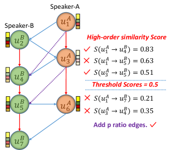
Figure 7: Example of adding $p$% high-order edges to explore global topological information of graph.

Appendix B Dimensions of Mathematical Symbols

Since we do not have much space to introduce details about the dimensions of the mathematical symbols in our main body. We carefully list all the dimensions of the mathematical symbols of IEMOCAP in Table 8. Mathematical symbols for other two datasets please see our source code.

Symbols	Description
$\bm{x}_{v}\in\mathbb{R}^{512}$	Video Features
$\bm{x}_{a}\in\mathbb{R}^{100}$	Audio Features
$\bm{x}_{t}\in\mathbb{R}^{768}$	Text Features
Contextual Representation Learning
$\bm{z}_{v}^{g}\in\mathbb{R}^{512}$	Global Hidden Video Features
$\bm{z}_{a}^{g}\in\mathbb{R}^{100}$	Global Hidden Audio Features
$\bm{z}_{t}^{g}\in\mathbb{R}^{768}$	Global Hidden Text Features
$\bm{z}_{m}^{g}\in\mathbb{R}^{1{,}380}$	Global Combined Features
$\bm{z}_{con}\in\mathbb{R}^{1,380}$	Topic-related Vector
$\bm{\hat{z}}_{m}^{g}\in\mathbb{R}^{1,380}$	Global Output Features
Specific Representation Learning
$\bm{z}_{v}^{\ell}\in\mathbb{R}^{460}$	Local Hidden Video Features
$\bm{z}_{a}^{\ell}\in\mathbb{R}^{460}$	Local Hidden Audio Features
$\bm{z}_{t}^{\ell}\in\mathbb{R}^{460}$	Local Hidden Text Features
$\bm{b}_{m}\in\mathbb{R}^{460}$	Basic Features
$\tilde{\bm{z}}_{\{v,a,t\}}^{\ell}\in\mathbb{R}^{460}$	Features in Shared Space
$\tilde{\bm{b}}_{m}\in\mathbb{R}^{460}$	Basic Features in Shared Space
$\textbf{W}_{\{v,a,t,b\}}\in\mathbb{R}^{460\times 460}$	Trainable Matrices
$\hat{\bm{z}}_{\{v,a,t\}}^{\ell}\in\mathbb{R}^{460}$	New Multimodal Features
$\hat{\bm{z}}_{m}^{\ell}\in\mathbb{R}^{1,380}$	New Multimodal Combined Features
$\bm{z}_{m}^{\ell}\in\mathbb{R}^{1380}$	Original Combined Features
Graph Contrastive Learning (One GCN Layer)
$(\hat{\bm{z}}_{g}^{\ell}\|\hat{\bm{z}}_{m}^{\ell})\in\mathbb{R}^{2,760}$	Global-Local Combined Features
$\textrm{AGG}\in\mathbb{R}^{2,760\times 2,760}$	Parameters of Aggregation Layer
$\textrm{COM}\in\mathbb{R}^{2,760\times 5,520}$	Input/Output of Combination Layer
$\textbf{W}_{graph}\in\mathbb{R}^{5,520\times 2,760}$	Dimention Reduction after COM
$\bm{h}_{m}\in\mathbb{R}^{2,760}$	Node Features of GCN Layer

Table 8: Mathematical symbols for IEMOCAP dataset.

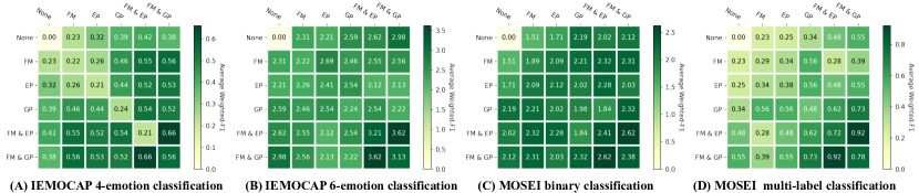
Figure 8: Average WF1 gain when contrasting different augmentation pairs, compared with training without graph augmentation module.

Appendix C Observations of Graph Augmentation

As shown in Figure 8, when we consider the combinations of (FM $\&$ EP) and (FP $\&$ GP) as two graph augmentation methods of the original graph, we could achieve the best performance. Furthermore, we have the following observations:

Obs.1: Graph augmentations are crucial.

Without any data augmentation, GCL module will not improve accuracy, judging from the averaged WF1 gain of the pair (None, None) in the upper left corners of Figure 8. In contrast, composing an original graph and its appropriate augmentation can benefit the averaged WF1 of emotion recognition, judging from the pairs (None, any) in the top rows or the left-most columns of Figure 8. Similar observation were in graphCL You et al. (2020), without augmentation, GCL simply compares two original samples as a negative pair with the positive pair loss becoming zero, which leads to homogeneously pushes all graph representations away from each other. Appropriate augmentations can enforce the model to learn representations invariant to the desired perturbations through maximizing the agreement between a graph and its augmentation.

Obs.2: Composing different augmentations benefits the model’s performance more.

Applying augmentation pairs of the same type does not often result in the best performance (see diagonals in Figure 8). In contrast, applying augmentation pairs of different types result in better performance gain (see off-diagonals of Figure 8). Similar observations were in SimCSE (Gao et al., 2021). As mentioned in that study, composing augmentation pairs of different types correspond to a “harder” contrastive prediction task, which could enable learning more generalizable representations.

Obs.3: One view having two augmentations result in better performance.

Generating each view by two augmentations further improve performance, i.e., the augmentations FM $\&$ EP, or FM $\&$ GP. The augmentation pair (FM $\&$ EP, FM $\&$ GP) results in the largest performance gain compared with other augmentation pairs. We conjectured the reason is that simultaneously changing structural and attribute information of the original graph can obtain more heterogeneous contextual information for nodes, which can be consider as “harder” example to prompt the GCL model to obtain more generalizable and robust representations.

P&F	Happiness	Sadness	Neutral	Anger	Accuracy	WF1
size=1	83.27	83.04	80.63	81.54	81.87	81.82
size=2	79.02	82.92	83.93	86.65	83.46	83.41
size=3	80.88	86.34	84.07	85.64	84.52	84.45
size=4	83.92	85.83	83.91	84.35	84.52	84.51
size=5	82.93	87.85	83.79	86.47	85.26	85.20
size=6	81.73	86.42	85.17	88.46	85.58	85.56
size=7	79.33	86.07	83.29	86.40	83.99	83.97
size=8	80.14	88.11	85.06	88.15	85.68	85.66
size=9	77.29	87.85	83.56	87.19	84.41	84.37
size=10	80.00	87.47	85.29	88.64	85.68	85.66
size=ALL	79.87	84.35	83.20	84.75	83.24	83.24

Table 9: Results for various window sizes for graph formation on the IEMOCAP (4-way).

P&F	Hap.	Sad.	Neu.	Ang.	Exc.	Fru.	Acc.	WF1
size=1	57.85	80.43	62.88	60.61	70.76	60.99	65.50	65.85
size=2	56.27	79.57	64.17	60.87	72.50	61.52	65.93	66.36
size=3	60.80	80.26	66.06	64.47	73.17	62.70	67.71	68.09
size=4	59.95	80.79	67.96	67.18	71.60	64.89	68.64	69.05
size=5	60.06	81.42	68.23	66.33	73.88	63.24	68.76	69.17
size=6	60.94	84.42	68.24	69.95	73.54	67.55	70.55	71.03
size=7	59.84	80.53	67.93	68.12	73.72	63.91	68.82	69.26
size=8	57.66	82.17	70.56	67.53	73.92	64.79	69.75	70.12
size=9	58.01	81.13	70.22	65.42	75.05	61.49	68.82	69.12
size=10	59.77	81.84	69.17	65.85	73.56	63.51	68.95	69.38
size=ALL	54.74	78.75	66.58	64.56	68.63	63.46	66.42	66.80

Table 10: Results for various window sizes for graph formation on the IEMOCAP (6-way).

Appendix D Parameters Sensitivity Study

In this section, we give more details about parameter sensitivity. First, as shown in Tables 9 & 10, when the window size $\in[6,8]$ for IEMOCAP (6-way) and the window size is 6 for IEMOCAP (4-way), Joyful achieved the best performance. A small window size will miss much contextual information, and a large-scale window size contains too much noise (topic will change over time). We set the window size for past and future to 6.

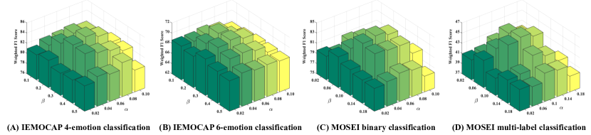
Figure 9: Parameters tuning for $\bm{\alpha}$ and $\bm{\beta}$ on validation datasets for all multimodal emotion recognition tasks.

Joyful also has two hyper-parameters: $\bm{\alpha}$ and $\bm{\beta}$, which balance the importance of MF module and GCL module in Eq.(15). Specifically, as shown in Figure 9, we observed how $\bm{\alpha}$ and $\bm{\beta}$ affect the performance of Joyful by varying $\bm{\alpha}$ from 0.02 to 0.10 in 0.02 intervals and $\bm{\beta}$ from 0.1 to 0.5 in 0.1 intervals. The results indicate that Joyful achieved the best performance when $\bm{\alpha}\in[0.06,0.08]$ and $\bm{\beta}\in[0.2,0.3]$ on IEMOCAP and and when $\bm{\alpha}\in[0.06,0.1]$ and $\bm{\beta}=0.1$ on MOSEI. The reason why these parameters can affect the results is that when $\bm{\alpha}$< 0.06, MF becomes weaker and representations contain too much noise, which cannot provide a good initialization for downstream MERC tasks. When $\bm{\alpha}$ >0.1, it tends to make reconstruction loss more important and Joyful tends to extract more common features among multiple modalities and loses attention to explore features from uni-modality. When $\bm{\beta}$ is small, graph contrastive loss becomes weaker, which leads to indistinguishable representation. A larger $\bm{\beta}$ wakes the effect of MF, leading to a local optimal solution. We set $\bm{\alpha}$=0.06 and $\bm{\beta}$=0.3 for IEMOCAP and MELD. We set $\bm{\alpha}$=0.06 and $\bm{\beta}$ =0.1 for MOSEI.

Method	Modality	WF1
IEMOCAP 6-way
CESTa	Text	67.10
SumAggGIN	Text	66.61
DiaCRN	Text	66.20
DialogXL	Text	65.94
DiaGCN	Text	64.18
COGMEN	Text	66.00
DAG-ERC	Fine-tune Text (RoBERTa-large)	68.03
Joyful	Text (Sentence-BERT)	67.48
	Text (RoBERTa-large)	68.05
	Fine-tune Text (RoBERTa-large)	68.45
	A+T+V	71.03

Table 11: Overall performance comparison on MOSEI with Text Modality.

Appendix E Uni-modal Performance

The focus of this study was multimodal emotion recognition. However, we also compared Joyful with uni-modal methods to evaluate its performance of joyful. We compared it with DAG-ERC (Shen et al., 2021b), CESTa (Wang et al., 2020), SumAggGIN (Sheng et al., 2020), DiaCRN (Hu et al., 2021), DialogXL (Shen et al., 2021a), DiaGCN (Ghosal et al., 2019), and COGMEN (Joshi et al., 2022). Following COGMEN, text-based models were specifically optimized for text modalities and incorporated changes to architectures to cater to text. As shown in Table 11, Joyful, being a fairly generic architecture, still achieved better or comparable performance with respect to the state-of-the-art uni-modal methods. Adding more information via other modalities helped to further improve the performance of Joyful (Text vs A+T+V). When using only text modality, the DAG-ERC baseline could achieve higher WF1 than Joyful. And we conjecture the main reasons is: DAG-ERC (Shen et al., 2021b) fine-tuned RoBERTa large model (Liu et al., 2019), with 354 million parameters, as their text encoder. By fine-tuning on RoBERTa large model under the guidance of downstream emotion recognition signals, RoBERTa large model can provide the most suitable text features for ERC. Compared with DAG-ERC, Joyful and other methods directly use Sentence-BERT (Reimers and Gurevych, 2019), with 110 million parameters, as their text encoder without fine-tuning on ERC datasets.

To verify whether the above inference is reasonable, we used RoBERTa large model as our text feature extractor called Text (RoBERTa-large). And we fine-tuned RoBERTa large model on the downstream IEMPCAP (6-way) dataset, following the same method of DAG-ERC called Fine-tune Text (RoBERTA-large). The observation meets our intuition. With RoBERTa large model, Joyful improved the performance (68.05 vs 67.48) compared with Sentence-BERT as our text encoder. And Joyful could obtain better performance (68.45 vs 68.03) in terms of WF1 than DAG-ERC with fine-tuned RoBERTa-large, demonstrating that fine-tuning large-scale model can help obtain richer text features to improve the performance. However, considering a fair comparison with other multimodal emotion recognition baselines (they do not have the fine-tuning process (Joshi et al., 2022; Ghosal et al., 2019)) and saving the additional time-consuming on fine-tuning, we directly adopt Sentence-BERT as our text encoder for IEMOCAP.

Appendix F Pseudo-Code of Joyful

As shown in Algorithm 1, to make Joyful easy to understand, we also provide a pseudo-code.

input : Visual features $\bm{x}_{v}$;

Audio features $\bm{x}_{a}$;

Text features $\bm{x}_{t}$;

Parameters: $\bm{\alpha}$, $\bm{\beta}$, Window size

output : Emotion recognition label.

Initialize trainable parameters;

for $epoch\leftarrow 1$ to $epoch\ num$ do

       Global Contextual Fusion $\hat{\bm{z}}_{m}^{g}$;

       Specific Modality Fusion $\hat{\bm{z}}_{m}^{\ell}$=($\bm{z}_{v}^{g}\|\bm{z}_{a}^{g}\|\bm{z}_{t}^{g}$);

       // Compute multimodal fusion loss

       Compute $\mathcal{L}_{mf}$, in accordance with Eq.(8);

       Feature Concatenation $\bm{h}=(\hat{\bm{z}}_{m}^{g}\|\hat{\bm{z}}_{m}^{\ell}$);

       Adopt $\bm{h}$ as initialization for Graph;

       // Generate two augmented views

       Apply FM & EP to generate view: $\mathcal{G}^{(1)}$;

       Apply FM & GP to generate view: $\mathcal{G}^{(2)}$;

       // Extract features of two views

       $\mathbf{H}^{(1)}$ = $GCNs(\mathcal{G}^{(1)})$, $\mathbf{H}^{(2)}$ = $GCNs(\mathcal{G}^{(2)})$ ;

       // Compute contrastive learning loss

       Compute $\mathcal{L}_{ct}$, in accordance with Eq.(13) ;

       // Aggregate extracted features

       $\mathbf{H}=\mathbf{H}^{(1)}+\mathbf{H}^{(2)}$ ;

       // Compute emotion recognition loss

       Compute $\mathcal{L}_{ce}$, in accordance with Eq.(14);

       // Joint training

       Compute $\mathcal{L}_{all}$, in accordance with Eq.(15);

       // Optimize with Adam optimizer

      

Adopt classifier on $\mathbf{H}$ to predict the emotional label.

Algorithm 1 Overall process of Joyful

Appendix G Benjamini-Hochberg Correction

Benjamini-Hochberg Correction (B-H) (Benjamini and Hochberg, 1995) is a powerful tool that decreases the false discovery rate. Considering the reproducibility of the multiple significant test, we introduce how we adopt the B-H correction and give the hyper-parameter values that we used. We first conduct a t-test (Yang et al., 1999) with default parameters to calculate the p-value between each comparison method with Joyful. We then put the individual p-values in ascending order as input to calculate the p-value corrected using the B-H correction. We directly use the “multipletests(*args)” function from python package and set the hyperparameter of the false discovery rate $Q=0.05$, which is a widely used default value (Puoliväli et al., 2020). Finally, we obtain a cut-off value as the output of the multipletests function, where cut-off is a dividing line that distinguishes whether two groups of data are significant. If the p-value is smaller than the cut-off value, we can conclude that two groups of data are significantly different.

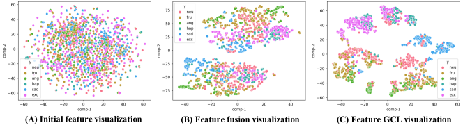
Figure 10: t-SNE visualization of IEMOCAP (6-way) features.

The use of t-test for testing statistical significance may not be appropriate for F-scores, as mentioned in Dror et al. (2018), as we cannot assume normality. To verify whether our data meet the normality assumption and the homogeneity of variances required for the t-test, following Shapiro and Wilk (1965) and Levene et al. (1960), we conducted the following validation. First, we performed the Shapiro-Wilk test on each group of experimental results to determine whether they are normally distributed. Under the constraint of a significance level (alpha=0.05), all p-values resulting from the Shapiro-Wilk test  for the baselines and our model were greater than 0.05. This indicates that the results of the baselines and our model all adhere to the assumption of normality. For example, in IEMOCAP-4, p-values for [Mult, RAVEN, MTAG, PMR, MICA, COGMEN, JOYFUL] are [0.903, 0.957, 0.858, 0.978, 0.970, 0.969, 0.862]. Furthermore, we used the Levene’s test Schultz (1985) to check for homogeneity of variances between baselines and our model. Under the constraint of a significance level (alpha = 0.05), we found that our p-values are greater than 0.05, indicating the homogeneity of the variances between the baselines and our model. For example, we obtained p-values 0.3101 and 0.3848 for group-based baselines on IEMOCAP-4 and IEMOCAP-6, respectively. Since we were able to demonstrate that all baselines and our model conform to the assumptions of normality and homogeneity of variances, we believe that the significance tests we reported are accurate.

Appendix H Representation Visualization

We visualized the node features to understand the function of the multimodal fusion mechanism and the GCL-based node representation learning component, as shown in Figure 10. Figure 10 (A) shows the concatenated multimodal features on the input side. Figure 10 (B) shows the representation of utterances after the feature fusion module. Figure 10 (C) shows the representation of the utterances after the GCL module (Eq.(10)) and before the pre-softmax layer (Eq.(11)). We observed that utterances could be roughly separated after the feature fusion mechanism, which indicates that the multimodal fusion mechanism can learn distinctive features to a certain extent. After GCL-based module, Joyful can be easily separated, demonstrating that GCL can provide distinguishable representation by exploring vertex attributes, graph structure, and contextual information from datasets.

Appendix I Labels Distribution of Datasets

In this section, we list the detailed label distribution of the three multimodal emotion recognition datasets MELD (Table 12), IEMOCAP 4-way (Table 13), IEMOCAP 6-way (Table 14) and MOSEI (Table 15) in the draft.

MELD	Train	Valid	Test
Anger	1,109	153	345
Disgusted	271	22	68
Fear	268	40	50
Joy	1,743	163	402
Neutral	4,710	470	1,256
Sadness	683	111	208
Surprise	1,205	150	281
Total	9,989	1,109	2,610

Table 12: Labels distribution of MELD dataset.

IEMOCAP 4-way	Train	Valid	Test
Happy	453	51	144
Sad	783	56	245
Neutral	1,092	232	384
Angry	872	61	170
Total	3,200	400	943

Table 13: Labels distribution of IEMOCAP 4-way.

IEMOCAP 6-way	Train	Valid	Test
Happy	459	45	144
Sad	746	93	245
Neutral	1,161	163	384
Angry	854	79	170
Excited	576	166	299
Frustrated	1,350	118	381
Total	5,146	644	1,623

Table 14: Labels distribution of IEMOCAP 6-way.

MOSEI	Train	Valid	Test
Happy	8,735	1,005	2,505
Sad	4,269	520	1,129
Angry	3,526	338	1,071
Surprise	1,642	203	441
Disgusted	2,955	281	805
Fear	1,331	176	385
Total	22,458	2,523	6,336

Table 15: Labels distribution of MOSEI dataset.

Case	Input modality			Target
	Text	Visual	Acoustic	MSA	MERC
Case A	Plot to it than that the action scenes were my favorite parts through it’s.	Smiling face Relaxed wink	Stress Pitch variation	+1.666	Positive
Case B	You must promise me that you’ll survive, you won’t give up.	Full of tears in his eyes	The voice is weak and trembling	-1.200	Negative

Table 16: Case study on the importance of each modality for MSA and MERC tasks. Blue in Text modality marks the contents including the strength of sentiments. Underline marks fragments contributing to the target on MERC.

Appendix J Multimodal Sentiment Analysis

We conducted experiments on two publicly available datasets, MOSI (Zadeh et al., 2016) and MOSEI (Zadeh et al., 2018), to investigate the performance of Joyful on the multimodal sentiment analysis (MSA) task.

Datasets: MOSI contains 2,199 utterance video segments, and each segment is manually annotated with a sentiment score ranging from -3 to +3 to indicate the sentiment polarity and relative sentiment strength of the segment. MOSEI contains 22,856 movie review clips from the YouTube website. Each clip is annotated with a sentiment score and an emotion label. And the exact number of samples for training/validation/test are 1,284/229/686 for MOSI and 16,326/1,871/4,659 for MOSEI.

Metrics: Following previous studies (Han et al., 2021a; Yu et al., 2021), we utilized evaluation metrics: mean absolute error (MAE) measures the absolute error between predicted and true values. Person correlation (Corr) measures the degree of prediction skew. Seven-class classification accuracy (ACC-7) indicates the proportion of predictions that correctly fall into the same interval of seven intervals between -3 and +3 as the corresponding truths. And binary classification accuracy (ACC-2) was computed for non-negative/negative classification results.

Baselines: We compared Joyful with three types of advanced multimodal fusion frameworks for the MSA task as follows, including current SOTA baselines MMIM (Han et al., 2021b) and BBFN (Han et al., 2021a): (1) Early multimodal fusion methods, which combine the different modalities before they are processed by any neural network models. We utilized Multimodal Factorization Model (MFM) (Tsai et al., 2019b), and Multimodal Adaptation Gate BERT (MAG-BERT) (Rahman et al., 2020) as baselines. (2) Late multimodal fusion methods, which combine the different modalities before the final decision or prediction layer. We utilized multimodal Transformer (MuIT) (Tsai et al., 2019a), and modal-temporal attention graph (MTAG) (Yang et al., 2021) as baselines. (3) Hybrid multimodal fusion methods combine early and late multimodal fusion mechanisms to capture the consistency and the difference between different modalities simultaneously. We utilized modality-invariant and modality-specific representations for MSA (MISA) (Hazarika et al., 2020), Self-Supervised multi-task learning for MSA (Self-MM) (Yu et al., 2021), Bi-Bimodal Fusion Network (BBFN) (Han et al., 2021a), and MultiModal InfoMax (MMIM) (Han et al., 2021b) as baselines.

Implementation Details: The results of proposed Joyful were averaged over ten runs using random seeds. We keep all hyper-parameters and implementations the same as in the MERC task reported in Sections 4.1 and 4.2. To make Joyful fit in the MSA task, we replace the current cross-entropy loss $\mathcal{L}_{ce}$ in Eq. (15) by mean absolute error loss $\mathcal{L}_{mae}$ as follows:

$$\mathcal{L}_{mae}=\frac{1}{m}\sum_{i=1}^{m}|\hat{y}_{i}-y_{i}|,$$ (16)

where $\hat{y}_{i}$ is the predicted value for the $i$-th sample, $y_{i}$ is the truth label for the $i$-th label, $m$ is the total number of samples, and $|\cdot|$ is the $L_{1}$ norm. We denote this model as Joyful+MAE.

Method	MOSI					MOSEI
	MAE $\downarrow$	Corr $\uparrow$	Acc-7 $\uparrow$	Acc-2 $\uparrow$		MAE $\downarrow$	Corr $\uparrow$	Acc-7 $\uparrow$	Acc-2 $\uparrow$
MFM	0.877	0.706	35.4	81.7		0.568	0.717	51.3	84.4
MAG-BERT	0.731	0.789	✗	84.3		0.539	0.753	✗	85.2
MulT	0.861	0.711	✗	84.1		0.580	0.703	✗	82.5
MTAG	0.866	0.722	0.389	82.3		✗	✗	✗	✗
MISA	0.804	0.764	✗	82.10		0.568	0.724	✗	84.2
Self-MM	0.713	0.789	✗	85.98		0.530	0.765	✗	85.17
BBFN	0.776	0.755	45.00	84.30		0.529	0.767	54.80	86.20
MMIM	0.700	0.800	46.65	86.06		0.526	0.772	54.24	85.97
Joyful+MAE	0.711	0.792	45.58	85.87		0.529	0.768	53.94	85.68

Table 17: Experimental results on the MOSI and MOSEI datasets. ✗ indicates unreported results. Bold indicates the least MAE, highest Corr, Acc-7, and Acc-2 scores for each dataset.

Experimental results on the MOSI and MOSEI datasets are listed in Table 17. Although the proposed Joyful could outperform most of the baselines (above the blue line), it performs worse than current SOTA models: BBFN and MMIM (below the blue line). We conjecture the main reasons are: when determining the strength of sentiments, compared with visual and acoustic modalities that may contain much noise data, text modality is more important for prediction (Han et al., 2021a). Table 16 lists such examples, where textual modality is more indicative than other modalities for the MSA task. Because the two baselines: BBFN (Han et al., 2021a) and MMIN (Han et al., 2021b), pay more attention to the text modality than visual and acoustic modalities during multimodal feature fusion, they may achieve low MAE, high Corr, Acc-2, and Acc-7. Specifically, BBFN (Han et al., 2021a) proposed a Bi-bimodal fusion network to enhance the text modality’s importance by only considered text-visual and text-acoustic interaction for features fusion. Conversely, considering the three modalities are all important for the MERC task as presented in Table 16, we designed Joyful to utilize the concatenation of the three modalities representations for prediction. Similar to our proposal, MISA and MAG-BERT considered the three modalities equally important during feature fusion but performed worse than SOTA baselines on the MSA task. In our consideration, because of such attention to modalities, Joyful outperformed SOTA baselines on the MERC task but underperformed SOTA baselines on the MSA task.

References

- Baltrusaitis et al. (2018) Tadas Baltrusaitis, Amir Zadeh, Yao Chong Lim, and Louis-Philippe Morency. 2018. Openface 2.0: Facial behavior analysis toolkit. In Proc. of FG, pages 59–66.
- Benjamini and Hochberg (1995) Yoav Benjamini and Yosef Hochberg. 1995. Controlling the false discovery rate: a practical and powerful approach to multiple testing. Journal of the Royal statistical society, 57(1):289–300.
- Busso et al. (2008) Carlos Busso, Murtaza Bulut, Chi-Chun Lee, Abe Kazemzadeh, Emily Mower, Samuel Kim, Jeannette N. Chang, Sungbok Lee, and Shrikanth S. Narayanan. 2008. IEMOCAP: interactive emotional dyadic motion capture database. Lang. Resour. Evaluation, 42(4):335–359.
- Chen et al. (2021) Zhihong Chen, Yaling Shen, Yan Song, and Xiang Wan. 2021. Cross-modal memory networks for radiology report generation. In Proc. of ACL/IJCNLP, pages 5904–5914.
- Dai et al. (2021) Wenliang Dai, Samuel Cahyawijaya, Zihan Liu, and Pascale Fung. 2021. Multimodal end-to-end sparse model for emotion recognition. In Proc. of NAACL-HLT, pages 5305–5316.
- Delbrouck et al. (2020) Jean-Benoit Delbrouck, Noé Tits, Mathilde Brousmiche, and Stéphane Dupont. 2020. A transformer-based joint-encoding for emotion recognition and sentiment analysis. In Workshop on Multimodal Language (Challenge-HML), pages 1–7.
- Devlin et al. (2019) Jacob Devlin, Ming-Wei Chang, Kenton Lee, and Kristina Toutanova. 2019. BERT: pre-training of deep bidirectional transformers for language understanding. In Proc. of NAACL-HLT, pages 4171–4186.
- Dror et al. (2018) Rotem Dror, Gili Baumer, Segev Shlomov, and Roi Reichart. 2018. The hitchhiker’s guide to testing statistical significance in natural language processing. In Proc. of ACL, pages 1383–1392.
- Eyben et al. (2010) Florian Eyben, Martin Wöllmer, and Björn Schuller. 2010. Opensmile: The munich versatile and fast open-source audio feature extractor. In Proc. of MM, page 1459–1462.
- Fu et al. (2021) Yahui Fu, Shogo Okada, Longbiao Wang, Lili Guo, Yaodong Song, Jiaxing Liu, and Jianwu Dang. 2021. CONSK-GCN: conversational semantic- and knowledge-oriented graph convolutional network for multimodal emotion recognition. In Proc. of ICME, pages 1–6.
- Gao et al. (2021) Tianyu Gao, Xingcheng Yao, and Danqi Chen. 2021. Simcse: Simple contrastive learning of sentence embeddings. In Proc. of EMNLP, pages 6894–6910.
- Ghosal et al. (2020) Deepanway Ghosal, Navonil Majumder, Alexander Gelbukh, Rada Mihalcea, and Soujanya Poria. 2020. COSMIC: COmmonSense knowledge for eMotion identification in conversations. In Findings of EMNLP, pages 2470–2481.
- Ghosal et al. (2019) Deepanway Ghosal, Navonil Majumder, Soujanya Poria, Niyati Chhaya, and Alexander Gelbukh. 2019. DialogueGCN: A graph convolutional neural network for emotion recognition in conversation. In Proc. of EMNLP-IJCNLP, pages 154–164.
- Guo et al. (2021) Xiaobao Guo, Adams Kong, Huan Zhou, Xianfeng Wang, and Min Wang. 2021. Unimodal and crossmodal refinement network for multimodal sequence fusion. In Proc. of EMNLP, pages 9143–9153.
- Gupta et al. (2022) Vikram Gupta, Trisha Mittal, Puneet Mathur, Vaibhav Mishra, Mayank Maheshwari, Aniket Bera, Debdoot Mukherjee, and Dinesh Manocha. 2022. 3massiv: Multilingual, multimodal and multi-aspect dataset of social media short videos. In Proc. of CVPR, pages 21032–21043.
- Hamilton et al. (2017) William L. Hamilton, Zhitao Ying, and Jure Leskovec. 2017. Inductive representation learning on large graphs. In Proc. of NeurIPS, pages 1024–1034.
- Han et al. (2021a) Wei Han, Hui Chen, Alexander F. Gelbukh, Amir Zadeh, Louis-Philippe Morency, and Soujanya Poria. 2021a. Bi-bimodal modality fusion for correlation-controlled multimodal sentiment analysis. In Proc. of ICMI, pages 6–15.
- Han et al. (2021b) Wei Han, Hui Chen, and Soujanya Poria. 2021b. Improving multimodal fusion with hierarchical mutual information maximization for multimodal sentiment analysis. In Proc. of EMNLP, pages 9180–9192.
- Hazarika et al. (2020) Devamanyu Hazarika, Roger Zimmermann, and Soujanya Poria. 2020. Misa: Modality-invariant and -specific representations for multimodal sentiment analysis. In Proc. of MM, page 1122–1131.
- Hu et al. (2022a) Dou Hu, Xiaolong Hou, Lingwei Wei, Lian-Xin Jiang, and Yang Mo. 2022a. MM-DFN: multimodal dynamic fusion network for emotion recognition in conversations. In Proc. of ICASSP, pages 7037–7041.
- Hu et al. (2021) Dou Hu, Lingwei Wei, and Xiaoyong Huai. 2021. DialogueCRN: Contextual reasoning networks for emotion recognition in conversations. In Proc. of ACL, pages 7042–7052.
- Hu et al. (2022b) Guimin Hu, Ting-En Lin, Yi Zhao, Guangming Lu, Yuchuan Wu, and Yongbin Li. 2022b. UniMSE: Towards unified multimodal sentiment analysis and emotion recognition. In Proc. of EMNLP, pages 7837–7851.
- Huang et al. (2017) Gao Huang, Zhuang Liu, Laurens van der Maaten, and Kilian Q. Weinberger. 2017. Densely connected convolutional networks. In Proc. of CVPR, pages 2261–2269.
- Ishiwatari et al. (2020) Taichi Ishiwatari, Yuki Yasuda, Taro Miyazaki, and Jun Goto. 2020. Relation-aware graph attention networks with relational position encodings for emotion recognition in conversations. In Proc. of EMNLP, pages 7360–7370.
- Jiao et al. (2020) Wenxiang Jiao, Michael R. Lyu, and Irwin King. 2020. Real-time emotion recognition via attention gated hierarchical memory network. In Proc. of AAAI, pages 8002–8009.
- Joshi et al. (2022) Abhinav Joshi, Ashwani Bhat, Ayush Jain, Atin Singh, and Ashutosh Modi. 2022. COGMEN: COntextualized GNN based multimodal emotion recognitioN. In Proc. of NAACL, pages 4148–4164.
- Katz (1953) Leo Katz. 1953. A new status index derived from sociometric analysis. Psychometrika, 18:39–43.
- Kim (2014) Yoon Kim. 2014. Convolutional neural networks for sentence classification. In Proc. of EMNLP, pages 1746–1751.
- Kingma and Ba (2015) Diederik P. Kingma and Jimmy Ba. 2015. Adam: A method for stochastic optimization. In Proc. of ICLR, pages 1–15.
- Kipf and Welling (2017) Thomas N. Kipf and Max Welling. 2017. Semi-supervised classification with graph convolutional networks. In Proc. of ICLR, pages 1–14.
- Le et al. (2022) Hung Le, Nancy Chen, and Steven Hoi. 2022. Multimodal dialogue state tracking. In Proc. of NAACL, pages 3394–3415.
- LeCun et al. (1995) Yann LeCun, Yoshua Bengio, et al. 1995. Convolutional networks for images, speech, and time series. The handbook of brain theory and neural networks, 3361(10):1995.
- Levene et al. (1960) Howard Levene et al. 1960. Contributions to probability and statistics. Essays in honor of Harold Hotelling, 278:292.
- Li et al. (2022a) Dongyuan Li, Jingyi You, Kotaro Funakoshi, and Manabu Okumura. 2022a. A-TIP: attribute-aware text infilling via pre-trained language model. In Proc. of COLING, pages 5857–5869.
- Li et al. (2022b) Sha Li, Madhi Namazifar, Di Jin, MOHIT BANSAL, Heng Ji, Yang Liu, and Dilek Hakkani-Tur. 2022b. Enhanced knowledge selection for grounded dialogues via document semantic graphs. In NAACL 2022.
- Li et al. (2022c) Shimin Li, Hang Yan, and Xipeng Qiu. 2022c. Contrast and generation make BART a good dialogue emotion recognizer. In Proc. of AAAI, pages 11002–11010.
- Li et al. (2022d) Shuangli Li, Jingbo Zhou, Tong Xu, Dejing Dou, and Hui Xiong. 2022d. Geomgcl: Geometric graph contrastive learning for molecular property prediction. In Proc. of AAAI, pages 4541–4549.
- Li et al. (2022e) Zhen Li, Bing Xu, Conghui Zhu, and Tiejun Zhao. 2022e. CLMLF:a contrastive learning and multi-layer fusion method for multimodal sentiment detection. In Findings of NAACL, pages 2282–2294.
- Liang et al. (2022) Sheng Liang, Mengjie Zhao, and Hinrich Schuetze. 2022. Modular and parameter-efficient multimodal fusion with prompting. In Findings of ACL, pages 2976–2985.
- Liang et al. (2021) Tao Liang, Guosheng Lin, Lei Feng, Yan Zhang, and Fengmao Lv. 2021. Attention is not enough: Mitigating the distribution discrepancy in asynchronous multimodal sequence fusion. In Proc. of ICCV, pages 8128–8136.
- Liang et al. (2023) Yunlong Liang, Fandong Meng, Jinan Xu, Jiaan Wang, Yufeng Chen, and Jie Zhou. 2023. Summary-oriented vision modeling for multimodal abstractive summarization. In Proc. of ACL, pages 2934–2951.
- Ling et al. (2022) Yan Ling, Jianfei Yu, and Rui Xia. 2022. Vision-language pre-training for multimodal aspect-based sentiment analysis. In Proc. of ACL, pages 2149–2159.
- Liu et al. (2020) Nayu Liu, Xian Sun, Hongfeng Yu, Wenkai Zhang, and Guangluan Xu. 2020. Multistage fusion with forget gate for multimodal summarization in open-domain videos. In Proc. of EMNLP, pages 1834–1845.
- Liu et al. (2019) Yinhan Liu, Myle Ott, Naman Goyal, Jingfei Du, Mandar Joshi, Danqi Chen, Omer Levy, Mike Lewis, Luke Zettlemoyer, and Veselin Stoyanov. 2019. Roberta: A robustly optimized BERT pretraining approach. CoRR, abs/1907.11692.
- Lv et al. (2021) Fengmao Lv, Xiang Chen, Yanyong Huang, Lixin Duan, and Guosheng Lin. 2021. Progressive modality reinforcement for human multimodal emotion recognition from unaligned multimodal sequences. In Proc. of CVPR, pages 2554–2562.
- Majumder et al. (2019) Navonil Majumder, Soujanya Poria, Devamanyu Hazarika, Rada Mihalcea, Alexander F. Gelbukh, and Erik Cambria. 2019. Dialoguernn: An attentive RNN for emotion detection in conversations. In Proc. of AAAI, pages 6818–6825.
- Mao et al. (2022) Huisheng Mao, Ziqi Yuan, Hua Xu, Wenmeng Yu, Yihe Liu, and Kai Gao. 2022. M-SENA: An integrated platform for multimodal sentiment analysis. In Proc. of ACL, pages 204–213.
- Nagrani et al. (2021) Arsha Nagrani, Shan Yang, Anurag Arnab, Aren Jansen, Cordelia Schmid, and Chen Sun. 2021. Attention bottlenecks for multimodal fusion. In Proc. of NeurIPS, pages 14200–14213.
- Nicolson et al. (2023) Aaron Nicolson, Jason Dowling, and Bevan Koopman. 2023. e-health CSIRO at radsum23: Adapting a chest x-ray report generator to multimodal radiology report summarisation. In The 22nd Workshop on BioNLP@ACL, pages 545–549.
- Ossowski and Hu (2023) Timothy Ossowski and Junjie Hu. 2023. Retrieving multimodal prompts for generative visual question answering. In Findings of the ACL.
- Partan and Marler (1999) Sarah Partan and Peter Marler. 1999. Communication goes multimodal. Science, 283(5406):1272–1273.
- Poria et al. (2019a) Soujanya Poria, Devamanyu Hazarika, Navonil Majumder, Gautam Naik, Erik Cambria, and Rada Mihalcea. 2019a. MELD: A multimodal multi-party dataset for emotion recognition in conversations. In Proc. of ACL, pages 527–536.
- Poria et al. (2021) Soujanya Poria, Navonil Majumder, Devamanyu Hazarika, Deepanway Ghosal, Rishabh Bhardwaj, Samson Yu Bai Jian, Pengfei Hong, Romila Ghosh, Abhinaba Roy, Niyati Chhaya, Alexander F. Gelbukh, and Rada Mihalcea. 2021. Recognizing emotion cause in conversations. Cogn. Comput., 13(5):1317–1332.
- Poria et al. (2019b) Soujanya Poria, Navonil Majumder, Rada Mihalcea, and Eduard H. Hovy. 2019b. Emotion recognition in conversation: Research challenges, datasets, and recent advances. IEEE Access, 7:100943–100953.
- Puoliväli et al. (2020) Tuomas Puoliväli, Satu Palva, and J. Matias Palva. 2020. Influence of multiple hypothesis testing on reproducibility in neuroimaging research: A simulation study and python-based software. Journal of Neuroscience Methods, 337:108654.
- Raguraman et al. (2019) Preeth Raguraman, Mohan Ramasundaram, and Midhula Vijayan. 2019. Librosa based assessment tool for music information retrieval systems. In Proc. of MIPR, pages 109–114.
- Rahman et al. (2020) Wasifur Rahman, Md. Kamrul Hasan, Sangwu Lee, AmirAli Bagher Zadeh, Chengfeng Mao, Louis-Philippe Morency, and Mohammed E. Hoque. 2020. Integrating multimodal information in large pretrained transformers. In Proc. of ACL, pages 2359–2369.
- Rajan et al. (2022) Vandana Rajan, Alessio Brutti, and Andrea Cavallaro. 2022. Is cross-attention preferable to self-attention for multi-modal emotion recognition? In Proc. of ICASSP, pages 4693–4697.
- Reimers and Gurevych (2019) Nils Reimers and Iryna Gurevych. 2019. Sentence-BERT: Sentence embeddings using Siamese BERT-networks. In Proc. of EMNLP-IJCNLP, pages 3982–3992.
- Scarselli et al. (2009) Franco Scarselli, Marco Gori, Ah Chung Tsoi, Markus Hagenbuchner, and Gabriele Monfardini. 2009. The graph neural network model. IEEE Trans. Neural Networks, 20(1):61–80.
- Schultz (1985) Brian B Schultz. 1985. Levene’s test for relative variation. Systematic Zoology, 34(4):449–456.
- Shankar (2022) Shiv Shankar. 2022. Multimodal fusion via cortical network inspired losses. In Proc. of ACL, pages 1167–1178.
- Shapiro and Wilk (1965) Samuel Sanford Shapiro and Martin B Wilk. 1965. An analysis of variance test for normality (complete samples). Biometrika, 52(3/4):591–611.
- Shazeer and Stern (2018) Noam Shazeer and Mitchell Stern. 2018. Adafactor: Adaptive learning rates with sublinear memory cost. In Proc. of ICML, volume 80, pages 4603–4611.
- Shen et al. (2021a) Weizhou Shen, Junqing Chen, Xiaojun Quan, and Zhixian Xie. 2021a. Dialogxl: All-in-one xlnet for multi-party conversation emotion recognition. In Proc. of AAAI, pages 13789–13797.
- Shen et al. (2021b) Weizhou Shen, Siyue Wu, Yunyi Yang, and Xiaojun Quan. 2021b. Directed acyclic graph network for conversational emotion recognition. In Proc. of ACL/IJCNLP, pages 1551–1560.
- Sheng et al. (2020) Dongming Sheng, Dong Wang, Ying Shen, Haitao Zheng, and Haozhuang Liu. 2020. Summarize before aggregate: A global-to-local heterogeneous graph inference network for conversational emotion recognition. In Proc. of COLING, pages 4153–4163.
- Shenoy et al. (2020) Aman Shenoy, Ashish Sardana, and et al. 2020. Multilogue-net: A context-aware RNN for multi-modal emotion detection and sentiment analysis in conversation. In Workshop on Multimodal Language (Challenge-HML), pages 19–28.
- Singh et al. (2022) Apoorva Singh, Soumyodeep Dey, Anamitra Singha, and Sriparna Saha. 2022. Sentiment and emotion-aware multi-modal complaint identification. In Proc. of AAAI, pages 12163–12171.
- Sun et al. (2022) Tiening Sun, Zhong Qian, Sujun Dong, Peifeng Li, and Qiaoming Zhu. 2022. Rumor detection on social media with graph adversarial contrastive learning. In Proc. of WWW, pages 2789–2797.
- Tan et al. (2022) Shiyin Tan, Jingyi You, and Dongyuan Li. 2022. Temporality- and frequency-aware graph contrastive learning for temporal network. In Proc. of CIKM, pages 1878–1888.
- Tsai et al. (2019a) Yao-Hung Hubert Tsai, Shaojie Bai, Paul Pu Liang, J. Zico Kolter, Louis-Philippe Morency, and Ruslan Salakhutdinov. 2019a. Multimodal transformer for unaligned multimodal language sequences. In Proc. of ACL, pages 6558–6569.
- Tsai et al. (2019b) Yao-Hung Hubert Tsai, Paul Pu Liang, Amir Zadeh, Louis-Philippe Morency, and Ruslan Salakhutdinov. 2019b. Learning factorized multimodal representations. In proc. of ICLR.
- Tsai et al. (2020) Yao-Hung Hubert Tsai, Martin Ma, Muqiao Yang, Ruslan Salakhutdinov, and Louis-Philippe Morency. 2020. Multimodal routing: Improving local and global interpretability of multimodal language analysis. In Proc. of EMNLP, pages 1823–1833.
- Wang et al. (2021) Tana Wang, Yaqing Hou, Dongsheng Zhou, and Qiang Zhang. 2021. A contextual attention network for multimodal emotion recognition in conversation. In Proc. of IJCNN, pages 1–7.
- Wang et al. (2020) Yan Wang, Jiayu Zhang, Jun Ma, Shaojun Wang, and Jing Xiao. 2020. Contextualized emotion recognition in conversation as sequence tagging. In Proc. of SIGDIAL, pages 186–195.
- Wang et al. (2019) Yansen Wang, Ying Shen, Zhun Liu, Paul Pu Liang, Amir Zadeh, and Louis-Philippe Morency. 2019. Words can shift: Dynamically adjusting word representations using nonverbal behaviors. In Proc. of AAAI, pages 7216–7223.
- Wang et al. (2022a) Yikai Wang, Xinghao Chen, Lele Cao, Wenbing Huang, Fuchun Sun, and Yunhe Wang. 2022a. Multimodal token fusion for vision transformers. In Proc. of CVPR, pages 12176–12185.
- Wang et al. (2023) Yusong Wang, Dongyuan Li, Kotaro Funakoshi, and Manabu Okumura. 2023. Emp: Emotion-guided multi-modal fusion and contrastive learning for personality traits recognition. In Proc. of ICMR, page 243–252.
- Wang (2022) Zhen Wang. 2022. Modern question answering datasets and benchmarks: A survey. CoRR, abs/2206.15030.
- Wang et al. (2022b) Zhen Wang, Xu Shan, Xiangxie Zhang, and Jie Yang. 2022b. N24news: A new dataset for multimodal news classification. In Proc. of LREC, pages 6768–6775.
- Wei et al. (2019) Yinwei Wei, Xiang Wang, Liqiang Nie, Xiangnan He, Richang Hong, and Tat-Seng Chua. 2019. MMGCN: multi-modal graph convolution network for personalized recommendation of micro-video. In Proc. of MM, pages 1437–1445.
- Wu et al. (2021) Yang Wu, Pengwei Zhan, Yunjian Zhang, LiMing Wang, and Zhen Xu. 2021. Multimodal fusion with co-attention networks for fake news detection. In Findings of the ACL/IJCNLP, pages 2560–2569.
- Xu et al. (2021) Dongkuan Xu, Wei Cheng, Dongsheng Luo, Haifeng Chen, and Xiang Zhang. 2021. Infogcl: Information-aware graph contrastive learning. In Proc. of NeurIPS, pages 30414–30425.
- Yang et al. (2021) Jianing Yang, Yongxin Wang, Ruitao Yi, Yuying Zhu, Azaan Rehman, Amir Zadeh, Soujanya Poria, and Louis-Philippe Morency. 2021. MTAG: modal-temporal attention graph for unaligned human multimodal language sequences. In Proc. of NAACL-HLT, pages 1009–1021.
- Yang et al. (1999) Yiming Yang, Xin Liu, and et al. 1999. A re-examination of text categorization methods. In Proc. of SIGIR, page 42–49.
- You et al. (2022) Jingyi You, Dongyuan Li, Manabu Okumura, and Kenji Suzuki. 2022. JPG - jointly learn to align: Automated disease prediction and radiology report generation. In Proc. of COLING, pages 5989–6001.
- You et al. (2020) Yuning You, Tianlong Chen, Yongduo Sui, Ting Chen, Zhangyang Wang, and Yang Shen. 2020. Graph contrastive learning with augmentations. In Proc. of NeurIPS, pages 1–12.
- Yu et al. (2021) Wenmeng Yu, Hua Xu, Ziqi Yuan, and Jiele Wu. 2021. Learning modality-specific representations with self-supervised multi-task learning for multimodal sentiment analysis. In Proc. of AAAI, pages 10790–10797.
- Zadeh et al. (2017) Amir Zadeh, Minghai Chen, Soujanya Poria, Erik Cambria, and Louis-Philippe Morency. 2017. Tensor fusion network for multimodal sentiment analysis. In Proc. of EMNLP, pages 1103–1114.
- Zadeh et al. (2018) Amir Zadeh, Paul Pu Liang, Soujanya Poria, Erik Cambria, and Louis-Philippe Morency. 2018. Multimodal language analysis in the wild: CMU-MOSEI dataset and interpretable dynamic fusion graph. In Proc. of ACL, pages 2236–2246.
- Zadeh et al. (2016) Amir Zadeh, Rowan Zellers, Eli Pincus, and Louis-Philippe Morency. 2016. Multimodal sentiment intensity analysis in videos: Facial gestures and verbal messages. IEEE Intelligent Systems, 31(6):82–88.
- Zeng and Xie (2021) Jiaqi Zeng and Pengtao Xie. 2021. Contrastive self-supervised learning for graph classification. In Proc. of AAAI, pages 10824–10832.
- Zhang et al. (2021) Dong Zhang, Xincheng Ju, Wei Zhang, Junhui Li, Shoushan Li, Qiaoming Zhu, and Guodong Zhou. 2021. Multi-modal multi-label emotion recognition with heterogeneous hierarchical message passing. In Proc. of AAAI, pages 14338–14346.
- Zhang et al. (2022) Yifei Zhang, Hao Zhu, Zixing Song, Piotr Koniusz, and Irwin King. 2022. COSTA: covariance-preserving feature augmentation for graph contrastive learning. In Proc. of KDD, pages 1–18.
- Zhang et al. (2023) Ying Zhang, Hidetaka Kamigaito, and Manabu Okumura. 2023. Bidirectional transformer reranker for grammatical error correction. In Findings of ACL, pages 3801–3825.
- Zhu et al. (2020) Yanqiao Zhu, Yichen Xu, Feng Yu, Qiang Liu, Shu Wu, and Liang Wang. 2020. Deep Graph Contrastive Representation Learning. In ICML Workshop on Graph Representation Learning and Beyond.