Is there a finite mobility for the one vibrational mode Holstein model? Implications from real time simulations

Abstract

The question of whether there exists a finite mobility in the standard Holstein model with one vibrational mode on each site remains unclear. In this letter, we approach this problem by employing the hierarchical equation of motion (HEOM) method to simulate model systems where the vibrational modes are dissipative. It is found that, as the friction becomes smaller, the charge carrier mobility increases significantly and a friction free limit can not be obtained. The current autocorrelation functions are also calculated for the friction free Holstein model, and converged results can not be obtained with the increase of the number of sites. Based on these observations, we conclude that a finite mobility can not be defined for the standard Holstein model, which is consistent with the recent finding by Kolss et al. (Phys. Rev. Lett. 123, 126601).

Charge carrier mobility is an important property of organic semiconducting materials, and is critical in many of their applications Tsutsui et al. (2016); Gershenson et al. (2006); Coropceanu et al. (2007). It is now well known that charge carrier transport in these materials are significantly affected by the electron-phonon interaction Holstein (1959a); Silbey and Munn (1980); Silinsh and Capek (1994); Troisi (2011). Depending on the strengths of the intermolecular electronic coupling and the electron-phonon coupling, the charge carrier transport mechanism can range from band-like behavior Farchioni (2001); Gershenson et al. (2006) to hopping transitions Nan et al. (2009), and cases in between Troisi and Orlandi (2006); Fratini et al. (2017); Li et al. (2021). As a unified theory is not yet available, charge carrier transport mechanism in organic materials continues to be an active area of theoretical research.

The Holstein modelHolstein (1959a, b) has been widely applied to study charge carrier transport in organic molecular crystals (OMCs), and has been indispensable in understanding such processes Cheng and Silbey (2008); Fetherolf et al. (2020). Analytically solutions of the Holstein model are only available in the strong and weak coupling limit Mahan (2000); Lang and Firsov (1963); Alexandrov and Devreese (2010). In the case of arbitrary coupling, approximate Berciu (2006); Zoli (2000); Cataudella et al. (1999) and numerically exact Mishchenko et al. (2008); Goodvin et al. (2011); Bonča et al. (1999); Jeckelmann and White (1998); Barišić (2004) methods can be employed. For example, quantum Monte Carlo (QMC) Kornilovitch (1998); Romero et al. (1998, 1999) simulation can be used to obtain imaginary time properties, while the charge carrier transport mobility can be obtained from an inverse Laplace transformation of the imaginary time results. The Green function methodsLangreth and Kadanoff (1964); Mahan (2000); Goodvin et al. (2011); Prodanović and Vukmirović (2019); Bonča et al. (2019); Mitrić et al. (2022); Mishchenko et al. (2015) can also be used to numerically simulate the Holstein model and obtain the charge carrier mobility.

Charge carrier mobility can also be obtained by calculating the real time current autocorrelation functions by using methods such as the density matrix renormalization group (DMRG) Jeckelmann and White (1998); Jansen et al. (2020); Li et al. (2020) approach. Since long time simulations are still very challenging, the correlation functions are usually truncated at a finite time. For this treatment to be valid, it is required that, either the long time behavior of the autocorrelation function is not important, or can be extrapolated using simple approximations.

A particularly interesting problem in the literature is the one vibrational mode Holstein model, where each site couples to a local vibrational mode. It is still not very clear whether there is a well defined diffusion constant for this problem when there is no static disorder or dissipation. In the literature, charge carrier mobilities have been obtained from both imaginary time and real time methods Troisi and Orlandi (2006); Troisi (2007); Wang et al. (2011a); Yan et al. (2019); Fetherolf et al. (2020). However, in a recent study of the friction free Holstein model by Kloss et al. Kloss et al. (2019), it is found that the mean square displacement (MSD) does not show a linear dependence of time $t$ for a wide range of parameters. This result indicates that a diffusion constant may not exist and thus the charge carrier transport mobility can not be defined for the standard one vibrational mode Holstein model.

In previous works, our group has employed the hierarchical equation of motion (HEOM) method to simulate the Holstein or Holstein-Peierls models Wang et al. (2010); Song and Shi (2015); Yan et al. (2019). The HEOM approach is a “numerically exact” method to simulate quantum dynamics in condensed phases Tanimura and Kubo (1989); Tanimura (2020), and is widely applied in different fields including excitation energy transfer (EET) dynamics and related spectroscopic phenomena Ishizaki and Fleming (2009); Yan et al. (2021), as well as nonequilibrium charge carrier transport dynamics Jin et al. (2008). In all our previous studies of the Holstein model Wang et al. (2010); Song and Shi (2015); Yan et al. (2019), dissipative modes were employed for the vibrational degrees of freedom (DOFs), and well defined diffusion constants and mobilities can be obtained.

In this work, we investigate whether a well defined mobility exists for the 1D one vibrational mode Holstein model, by starting from a 1D Holstein model with dissipation and systematically decreasing the dissipation strength towards the friction free limit. More specifically, we apply the methods previously developed in Refs. Li et al. (2022); Xing et al. (2022) to a Holstein model with a Brownian oscillator (BO) spectral density, where the strength of dissipation is controlled by a single parameter. Charge carrier mobilities for the dissipative model are then calculated from both the MSD and the real time current autocorrelation functions, and extrapolated to the friction free limit.

We start from the total Hamiltonian for a standard 1D single mode Holstein model, which is given by Holstein (1959a):

$$\hat{H}_{S}=\hat{H}_{e}+\hat{H}_{vib}+\hat{H}_{e-vib}\;\;.$$ (1)

Here, the electronic Hamiltonian $\hat{H}_{e}$ is defined as:

$$\hat{H}_{e}=-J\sum_{n}\left({\hat{c}}^{\dagger}_{n+1}{\hat{c}}_{n}+{\hat{c}}^{\dagger}_{n}{\hat{c}}_{n+1}\right)\;\;,$$ (2)

where the $\hat{c}^{\dagger}_{n}$ and $\hat{c}_{n}$ are the creation and annihilation operators of the electron at site $n$, $J$ is the electronic coupling between nearest neighbors.

The phonon Hamiltonian $\hat{H}_{vib}$ is given by:

$$\hat{H}_{vib}=\Omega\sum_{n}{\hat{b}}^{\dagger}_{n}{\hat{b}}_{n}\;\;,$$ (3)

where the $\hat{b}^{\dagger}_{n}$ and ${\hat{b}}_{n}$ are the creation and annihilation operators of the vibrational mode at site $n$ with frequency $\Omega$.

The interaction term is defined as,

$$\hat{H}_{e-vib}=C\sum_{n}\left(\hat{b}^{\dagger}_{n}+\hat{b}_{n}\right)\hat{c}^{\dagger}_{n}\hat{c}_{n}\;\;,$$ (4)

where $C$ is the coupling constant between the electronic DOF and the vibrational mode.

As stated above, we first simulate a model system where the vibrational modes are subjected to dissipation. To this end, each vibrational mode is coupled to a set of harmonic oscillators, such that the total bath Hamiltonian is written as:

$$\hat{H}_{B}=\sum_{n}\sum_{m}\left(\frac{\hat{p}_{n,m}^{2}}{2M_{n,m}}+\frac{1}{2}M_{n,m}\omega_{n,m}^{2}\hat{x}_{n,m}^{2}\right)\;\;,$$ (5)

where $\hat{p}_{n,j}$, $\hat{x}_{n,j}$, $M_{n,j}$, and $\omega_{n,j}$ are the momentum, position, mass, and frequency of the $j$th oscillator of $n$th site.

The interaction between the vibrational modes and harmonic bath is given by:

$$\hat{H}_{I}=\sum_{n}\sum_{m}\left({\hat{b}}^{\dagger}_{n}+{\hat{b}}_{n}\right)\hat{x}_{n,m}\;\;.$$ (6)

The total Hamiltonian of the dissipative Holstein model is then $\hat{H}_{tot}=\hat{H}_{S}+\hat{H}_{B}+\hat{H}_{I}$. The vibrational part of the total Hamiltonian $\hat{H}_{vib}+\hat{H}_{B}$ + $\hat{H}_{I}$ can be diagonalized into a new set of harmonic oscillator modes:

$$\hat{H}^{\prime}_{vib}=\sum_{n}\sum_{j}\omega^{\prime}_{n,j}\hat{b}^{\prime\dagger}_{n,j}\hat{b}^{\prime}_{n,j}\;\;.$$ (7)

By using this new sets of harmonic oscillator modes, the electron-phonon interaction term can be written as

$$\hat{H}^{\prime}_{e-vib}=\sum_{n}\hat{F}_{n}\hat{c}^{\dagger}_{n}\hat{c}_{n}\;\;,$$ (8)

where

$$\hat{F}_{n}=\sum_{j}g_{n,j}(\hat{b}^{\prime\dagger}_{n,j}+\hat{b}^{\prime}_{n,j})\;\;.$$ (9)

The spectral density for the $n$th site is defined as Weiss (2012); Garg et al. (1985),

$$J_{n}(\omega)=\frac{\pi}{2}\sum_{j}\frac{g_{n,j}^{2}}{\omega^{\prime}_{n,j}}\delta(\omega-\omega^{\prime}_{n,j})\;\;.$$ (10)

The above procedure to turn a problem from a system-vibrational mode-harmonic bath model into a new effective system-harmonic bath model has been introduced by Leggett, Garg $et\;al$. Leggett (1984); Garg et al. (1985). In this work, we assume that the spectral density is the same for all sites, and takes the following form:

$$J(\omega)=\lambda\frac{\Omega^{2}\gamma\omega}{(\omega^{2}-\Omega^{2})^{2}+4\gamma^{2}\omega^{2}}\;\;.$$ (11)

The so called Brownian oscillator (BO) spectral density in Eq. (11) can be derived by coupling a harmonic oscillator to an Ohmic bath Leggett (1984); Garg et al. (1985); Ito and Tanimura (2016); Tanaka and Tanimura (2009).

In Eq. (11), the reorganization energy is determined by the vibrational frequency $\Omega$ and the coupling constant $C$ in Eqs. (3) and (4) as $\lambda=C^{2}/\Omega^{2}$. So, the parameter $\gamma$ in Eq.(11) actually controls the strength of the dissipative effects. To study effects of dissipation on the charge carrier mobility, we choose to fix the vibrational frequency $\Omega$ and reorganization energy $\lambda$, and investigate how $\gamma$ affects the charge carrier transport. FIG. S1 in the supporting information shows the BO spectral density $J(\omega)$ for different values of $\gamma$, with $\lambda=1.0$ and $\Omega=2.0$. It can be seen that the shape of $J(\omega)$ changes significantly as $\gamma$ varies. When $\gamma=0$, $J(\omega)$ is a delta function, corresponding to the standard friction free 1D Holstein model. As $\gamma$ increases, $J(\omega)$ is broadened and the position of the peak shifts to lower frequencies. When $0<\gamma<\Omega$, the system is underdamped, and when $\gamma>\Omega$ the system is overdamped.

The charge carrier mobility of the dissipative Holstein model is obtained by using two different approaches. The first one is based on starting from an initial state and obtain the MSD using real time propagation:

$${\rm MSD}(t)=\sum_{j=1}^{N}j^{2}P_{j}(t)\;\;,$$ (12)

where $P_{j}$ is the population of the $j$th site.

The diffusion constant $D$ is then obtained when the MSD reaches the linearly growth region:

$$D=\frac{1}{2}\lim_{t\to\infty}\frac{d{\rm MSD}(t)}{dt}\;\;.$$ (13)

The charge carrier mobility is then obtained by the Einstein relation: $\mu=eD/k_{B}T$ Kubo et al. (1995), where $k_{B}$ is the Boltzmann constant, $T$ is the temperature.

Another approach to calculate the charge carrier mobility is based on the Green-Kubo relation Mahan (2000):

$$\mu=\frac{1}{2k_{B}T}\lim_{\omega\to 0}\int_{-\infty}^{\infty}dte^{i\omega t}\langle\hat{j}(t)\hat{j}(0)\rangle\;\;,$$ (14)

where the current operator $\hat{j}$ in the Holstein model is given by

$$\hat{j}=-iJ\sum_{m}({\hat{c}}^{\dagger}_{m+1}{\hat{c}}_{m}-{\hat{c}}^{\dagger}_{m}{\hat{c}}_{m+1})\;\;.$$ (15)

To obtain the current autocorrelation function $\langle\hat{j}(t)\hat{j}(0)\rangle$, we first use the imaginary time HEOM to calculate the correlated initial state, i.e., the equilibrium $\tilde{\rho}_{\bf n}$ . The current operator $\hat{j}$ is then multiplied to the equilibrium $\tilde{\rho}_{\bf n}$ and the new quantities $\hat{j}\tilde{\rho}_{\bf n}$ is used as the initial state to propagate the real time HEOM. Finally, we multiple the current operator to the reduced density operator at time $t$, and trace over the electron DOFs to obtain the correlation function $\langle\hat{j}(t)\hat{j}(0)\rangle$. The exact form and details of the real and imaginary time HEOM can be found in the supporting information.

By applying proper approximations, the current autocorrelation function can also be calculated analytically. When the electronic coupling constant $J$ is much smaller than the reorganization energy $\lambda$, by applying the second order perturbation with respect to $J$, the current autocorrelation function can be calculated as Wang et al. (2011b):

$$C(t)\approx 2J^{2}{\rm Re}\exp\{-g(t)\}\;\;,$$ (16)

where

$$g(t)=\frac{2}{\pi\hbar}\int d\omega\frac{J(\omega)}{\omega^{2}}\{\coth(\beta\hbar\omega/2)[1-\cos(\omega t)]+i\sin(\omega t)\}\;\;.$$ (17)

This equation is used to help analyzing the simulation results when $J$ is small.

By applying the real time HEOM, we first calculate the MSD for the dissipative Holstein model. The periodic boundary condition is employed, and two different sets of parameter are used in the simulation. In the first set of parameters, $\lambda=1.0,\Omega=1.0,\beta=1.0$, and $J=0.1$. Since the reorganization energy $\lambda$ is significantly larger than the electronic coupling constant $J$, it is supposed to be in the strong electron-phonon coupling regime. Five different values for the friction parameter $\gamma=$ $0.05,0.2,0.5,0.8,1.5$ are used in the simulation, where the first four are in the underdamped regime ($\gamma<1.0$), and the last one is in the the overdamped regime ($\gamma>1.0$).

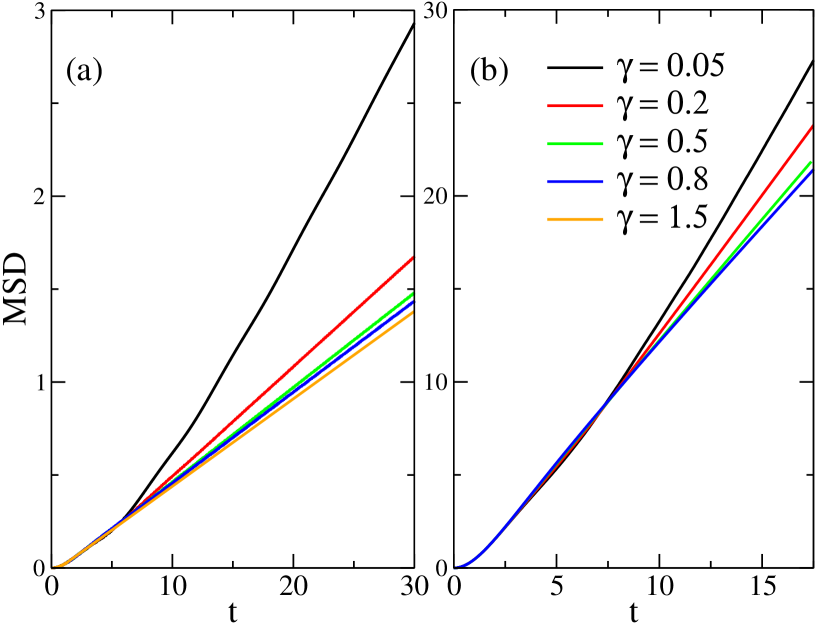
Figure 1: MSD simulated by the HEOM method for different values of $\gamma$: (a) $J=0.1$, (b) $J=0.5$. The other parameters are $\lambda$ = 1.0, $\Omega$ = 1.0, and $\beta$ = 1.0.

The initial state of the real time HEOM simulation is $|0\rangle\langle 0|\otimes e^{-\beta\hat{H}_{vib}}$. The total number of sites used in the simulation is up to 21 depending on different values of $\gamma$, ensuring that the MSD has reached the linear growth region and the calculated diffusion constant is not affected by boundary effects. The HEOM simulation is based on the matrix product state(MPS) method with bond dimension of 80. The simulated MSD is shown in Fig. 1(a). It can be seen that, with the increase of the the friction constant $\gamma$, the slope of the MSD curve becomes smaller. Besides, the time to reach the linear growth region of the MSD also increases with the decrease of $\gamma$.

In another set of parameters, we use $\lambda=1.0$, $\Omega=1.0$, $\beta=1.0$, and $J=0.5$. Since the reorganization energy $\lambda$ and the electronic coupling constant $J$ are now comparable in magnitude, this is a case in the so called intermediate coupling regime. As the coupling constant $J$ is now much larger than that in the first set of parameters, the real time HEOM propagation becomes more challenging. To obtain converged results, the number of sites needed is 51 for $\gamma=1.5$, and 71 for $\gamma=0.05$. Bond dimension for the MPS also increases to 120. The time dependent MSD obtained for the second set of parameters is presented in Fig. 1(b). Same as the $J=0.1$ case, for smaller $\gamma$ values, it takes a longer time for the MSD to reach the linear growth region. The diffusion constants are also larger for small $\gamma$.

We then apply the imaginary and real time HEOM to simulate the current autocorrelation function for the aforementioned two sets of parameters. The MPS method is applied to propagate imaginary time HEOM, with bond dimension of 90 for all different $\gamma$s. The cosine fitting scheme with seven cosine terms is used to fit the imaginary time bath correlation function Xing et al. (2022). To obtain converged results, the numbers of sites used in the simulations are from 8 ($\gamma=0.8$) to 10 ($\gamma=0.05$) for $J=0.1$, and 10 ($\gamma=0.8$) to 26 ($\gamma=0.05$) for $J=0.5$. FIG. S3 in the supporting information shows the convergence of the current autocorrelation function with respect to different number of sites when $\gamma=0.05$, $J$=0.5.

In the $J=0.1$ case, the current autocorrelation functions for different values of $\gamma$ are shown in Fig. 2(a), and the comparison with the second order perturbation is shown in Fig. S4 in the supporting information. The current autocorrelation functions for $J$ = 0.5 are shown in Fig. 2(b) and Fig. S5. In both cases, faster decay of the correlation function is observed when increasing $\gamma$. It is also shown that, for larger coupling constant $J$, the current autocorrelation function becomes less oscillatory.

For all values of $\gamma$ and $J$, the current autocorrelation function decays to zero, which indicates that a finite mobility can be obtained via the Green-Kubo relation in Eq. (14). The second order perturbation results in Fig. S4 and Fig. S5 also show that, although the accuracy of the second order autocorrelation functions depends on specific model parameters, they also decay to zero and leads a finite approximate mobility.

The mobilities calculated by using the MSD method and the Green-Kubo relation are consistent with each other. Fig. 3(a) shows the calculated mobilities via the MSD and the Green-Kubo relation, compared with the second order perturbation theory for $J=0.1$. It can be seen that, the mobility decreases when the dissipation becomes stronger. The second order perturbation actually works very well for large frictions, but overestimates the mobility at low friction. The same behavior is observed in the results for $J=0.5$ shown in Fig. 3(b), although the overestimation is rather pronounced for small friction ($\gamma=0.05$). It is thus shown that the friction constant $\gamma$ plays an important role in charge transport. Increasing $\gamma$ leads to stronger decoherence, which makes the current autocorrelation function decaying faster to zero, and reduces the mobility.

However, when we try to extrapolate the results to the friction free limit by taking $\gamma\rightarrow 0$, the $\gamma=0$ limit can not be defined in both the $J=0.1$ and 0.5 cases because of the sharp decrease of the mobility for small $\gamma$s. I.e., the mobility tends to diverge when $\gamma\rightarrow 0$. The divergence of the second order perturbation result is actually easy to understand: As shown in Fig. S6, in the case $\gamma=0$, the second order current autocorrelation function calculated via Eq. (16) a periodic function with the period of $2\pi/\Omega$, so the integration in the Green-Kubo relation goes to infinity.

It would then be interesting to investigate how the current autocorrelation functions in the friction free Holstein model behave beyond the second order perturbation. We now apply the combined imaginary and real time HEOM towards this problem. For the friction free Holstein model, the imaginary time bath (vibrational) correlation function is expanded analytically by hyperbolic functions Xing et al. (2022).

The current autocorrelation functions for the friction free model with different number of sites are shown in Fig. 4. The parameters used in the simulation are $\lambda=1.0$, $\Omega=1.0$, $\beta=1.0$, $\gamma=0$, and $J=0.5$. It can be seen that, the HEOM current autocorrelation function does not converge even for a large number of sites ($N$=50). However, compared with the second order result shown in Fig. S6, the HEOM correlation function also does not show significant recurrences. So, based on above characteristic of the friction free current autocorrelation function, and the failure to extrapolate the mobilities in the dissipative model to the zero friction limit, we conclude that a finite mobility may not be obtained for the friction free one vibrational mode Holstein model.

In summary, we have applied the imaginary and real time HEOM to simulate the MSD and current autocorrelation function for the 1D single mode Holstein model. The main observation is that, with dissipative vibrational modes, the current autocorrelation function decays to zero, such that a finite mobility can be obtained. On the other hand, in the friction free Holstein model, the current autocorrelation function does not decay to zero, and a finite mobility cannot be defined either from the Green-Kubo relation, or via extrapolation from finite friction results. This is consistent with the recent finding that no diffusive behavior can be observed from the MSD of the friction free Holstein model Kloss et al. (2019). Of course, in realistic systems, dissipation and static disorderChuang and Cao (2021) are unavoidable, and a finite mobility should always be obtained.

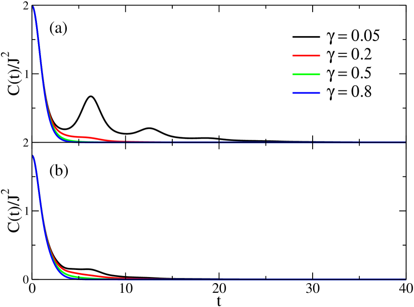
Figure 2: Current autocorrelation function simulated by the HEOM method for different values of $\gamma$: (a) $J=0.1$, (b) $J=0.5$.

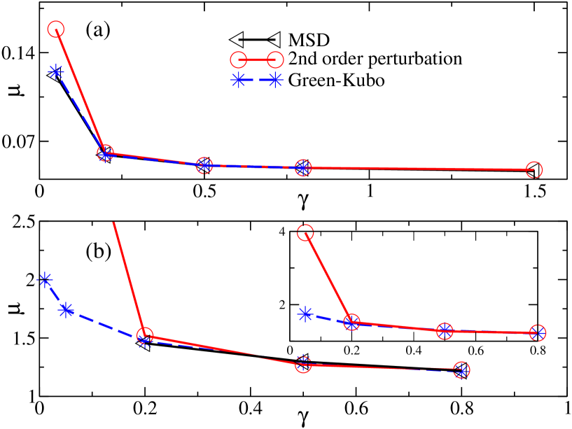
Figure 3: The mobility simulated by the HEOM method using the MSD and current autocorrelation function, compared with the second order perturbation result. (a) $J=0.1$, (b) $J=0.5$.

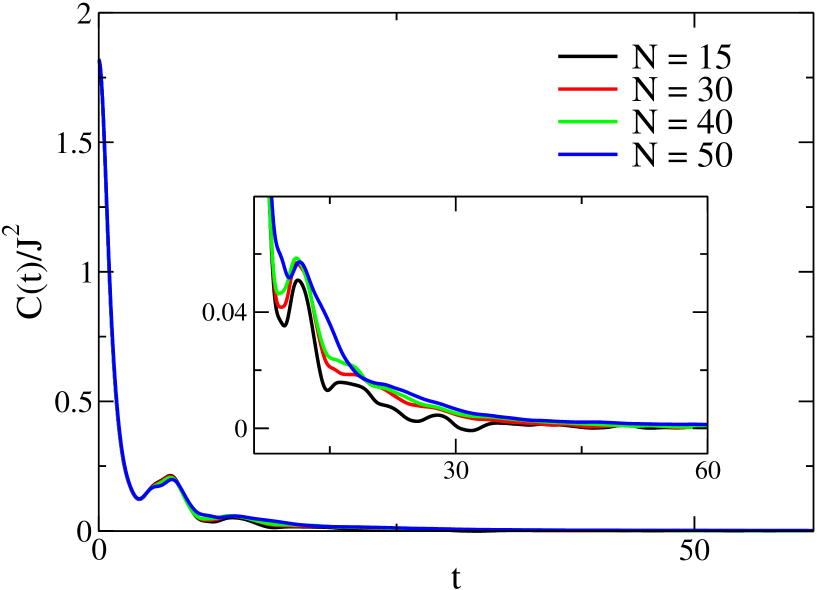
Figure 4: Current autocorrelation functions simulated by the HEOM method for the friction free Holstein model. The parameters used in the simulations are $\lambda$ = 1.0, $\Omega$ = 1.0, $J$ = 0.5, and $\beta$ = 1.0.