Abstract

Score-based generative models (SGMs) is a recent class of deep generative models with state-of-the-art performance in many applications. In this paper, we establish convergence guarantees for a general class of SGMs in 2-Wasserstein distance, assuming accurate score estimates and smooth log-concave data distribution. We specialize our result to several concrete SGMs with specific choices of forward processes modelled by stochastic differential equations, and obtain an upper bound on the iteration complexity for each model, which demonstrates the impacts of different choices of the forward processes. We also provide a lower bound when the data distribution is Gaussian. Numerically, we experiment SGMs with different forward processes, some of which are newly proposed in this paper, for unconditional image generation on CIFAR-10. We find that the experimental results are in good agreement with our theoretical predictions on the iteration complexity, and the models with our newly proposed forward processes can outperform existing models.

Wasserstein Convergence Guarantees for a General Class of Score-Based Generative Models

Xuefeng Gao , Hoang M. Nguyen , Lingjiong Zhu 

1 Introduction

Diffusion models are a powerful family of probabilistic generative models which can generate approximate samples from high-dimensional distributions [SDWMG15, SE19, HJA20]. The key idea in diffusion models is to use a forward process to progressively corrupt samples from a target data distribution with noise and then learn to reverse this process for generation of new samples. Diffusion models have achieved state-of-the-art performance in various applications such as image and audio generations, and they are the main components in popular content generators including Stable Diffusion [RBL⁺22] and Dall-E 2 [RDN⁺22]. We refer the readers to [YZS⁺22, CHIS23] for comprehensive surveys on diffusion models.

A predominant formulation of diffusion models is score-based generative models (SGM) through Stochastic Differential Equations (SDEs) [SSDK⁺21], referred to as Score SDEs in [YZS⁺22]. At the core of this formulation there are two stochastic processes in $\mathbb{R}^{d}$: a forward process and a reverse process. In this paper, we consider a general class of forward process $(\mathbf{x}_{t})_{t\in[0,T]}$ described by the following SDE:

$$d\mathbf{x}_{t}=-f(t)\mathbf{x}_{t}dt+g(t)d\mathbf{B}_{t},\quad\mathbf{x}_{0}\sim p_{0},$$ (1.1)

where both $f(t)$ and $g(t)$ are scalar-valued non-negative continuous functions of time $t$, $(\mathbf{B}_{t})$ is the standard $d$-dimensional Brownian motion, and $p_{0}$ is the (unknown) target data distribution. The forward process has the interpretation of slowly injecting noise to data and transforming them to a noise-like distribution. If we reverse the forward process (1.1) in time, i.e., letting $(\tilde{\mathbf{x}}_{t})_{t\in[0,T]}=(\mathbf{x}_{T-t})_{t\in[0,T]}$, then under mild assumptions, the reverse process $(\tilde{\mathbf{x}}_{t})_{t\in[0,T]}$ satisfies another SDE (see e.g. [And82, CCGL23]):

$$d\tilde{\mathbf{x}}_{t}=\left[f(T-t)\tilde{\mathbf{x}}_{t}+(g(T-t))^{2}\nabla_{\mathbf{x}}\log p_{T-t}(\tilde{\mathbf{x}}_{t})\right]dt+g(T-t)d\bar{\mathbf{B}}_{t},\quad\tilde{\mathbf{x}}_{0}\sim p_{T},$$ (1.2)

where $p_{t}(\mathbf{x})$ is the probability density function of $\mathbf{x}_{t}$ (the forward process at time $t$), $(\bar{\mathbf{B}}_{t})$ is a standard Brownian motion in $\mathbb{R}^{d}$ and $\tilde{\mathbf{x}}_{T}=\mathbf{x}_{0}\sim p_{0}$. Hence, the reverse process (1.2) transforms a noise-like distribution $p_{T}$ into samples from $p_{0}$, which is the goal of generative modeling. Note that the reverse SDE (2.2) involves the score function, $\nabla_{\mathbf{x}}\log p_{t}(\mathbf{x})$, which is unknown. An important subroutine in SGM is to estimate this score function based on samples drawn from the forward process, typically by modelling time-dependent score functions as neural networks and training them on certain score matching objectives [HD05, Vin11, SGSE20]. After the score is estimated, one can numerically solve the reverse SDE to generate new samples that approximately follows the data distribution (see Section 2). The Score-SDEs formulation is attractive because it generalizes and unifies several well-known diffusion models. In particular, the noise perturbation in Score Matching with Langevin dynamics (SMLD) [SE19] corresponds to the discretization of so-called variance exploding (VE) SDEs where $f\equiv 0$ in (1.1); The noise perturbation in Denoising Diffusion Probabilistic Modeling (DDPM) [SDWMG15, HJA20] corresponds to an appropriate discretization of the variance preserving (VP) SDEs where $f(t)=\frac{1}{2}\beta(t)$ and $g(t)=\sqrt{\beta(t)}$ for some noise variance schedule $\beta(t)$, see [SSDK⁺21] for details.

Despite the impressive empirical performances of diffusion models in various applications, the theoretical understandings of these models are still limited. In the past three years, there has been a rapidly growing body of literature on the convergence theory of diffusion models, assuming access to accurate estimates of the score function, see e.g. [BMR20, DBTHD21, DB22, LLT22, LLT23, CLL23, CCL⁺23, LWCC23, CDD23, BDBDD23]. While (some of) these studies have established polynomial convergence bounds for fairly general data distribution, this line of work has mostly focused on the analysis of the DDPM model where the corresponding forward SDE (1.1) satisfies $f=g^{2}/{2}>0$ (in fact many studies simply consider $f\equiv 1/2$ and $g\equiv 1$). However, it is important to understand the impacts of different choices of forward processes in diffusion models, which can potentially help provide theoretical guidance for selecting the functions $f$ and $g$ in the design of diffusion models. In this work, we make some initial progress towards addressing these issues using a theoretical approach based on convergence analysis. We summarize our contributions below.

Our Contributions.

• We establish convergence guarantees for a general class of SGMs in 2-Wasserstein distance, assuming accurate score estimates and smooth log-concave data distribution (Theorem 5). In particular, we allow general functions $f$ and $g$ in the forward SDE (1.1). Theorem 5 directly translates to an upper bound on the iteration complexity, which is the number of sampling steps/iterations needed (in running the reverse process) to yield $\epsilon-$accuracy in 2-Wasserstein distance between the data distribution and the generative distribution of the SGMs.

• We specialize our result to SGMs with specific functions $f$ and $g$ in the forward process. We find that under mild assumptions, the class of VP-SDEs (as forward processes) will always lead to an iteration complexity bound $\widetilde{\mathcal{O}}\left(d/\epsilon^{2}\right)$ where $\widetilde{\mathcal{O}}$ ignores the logarithmic factors and hides dependency on other parameters. On the other hand, in the class of VE-SDEs, the choice of an exponential function $g$ in [SE19, SSDK⁺21] leads to an iteration complexity of $\widetilde{\mathcal{O}}\left(d/\epsilon^{2}\right)$, while other simple choices including polynomials for $g$ lead to a worse complexity bound. We also find that VP-SDEs with polynomial and exponential noise schedules, which appear to be new to the literature, lead to better iteration complexity bounds (in terms of logarithmic dependence on $d,\epsilon$) compared with the existing models. See Table 2 and Proposition 6.

• We establish two results on lower bounds. We first show that if we use the upper bound in Theorem 5, then in order to achieve $\epsilon$ accuracy, the iteration complexity is $\widetilde{\Omega}\left(d/\epsilon^{2}\right)$ for quite general functions $f$ and $g$, where $\widetilde{\Omega}$ ignored the logarithmic dependence on $\epsilon$ and $d$ (Proposition 7). This result, however, does not show whether our upper bound in Theorem 5 is tight or not. We next show that if the data distribution $p_{0}$ is a Gaussian distribution, then the lower bound for the iteration complexity is $\Omega\left(\sqrt{d}/\epsilon\right)$ (Proposition 8). We do not know what the lower bound is when the data distribution is non Gaussian, partly because the score function needs to be estimated in this case and it is difficult to explicitly bound the 2-Wasserstein distance between two general distributions. See Section 3.2 for detailed discussions.

• Numerically, we experiment SGMs with different forward SDEs for unconditional image generation on the CIFAR-10 image dataset, using the neural network architectures from [SSDK⁺21]. We find that the experimental results are in good agreement with our theoretical predictions: models with lower order of iteration complexity generally perform better, in the sense that they achieve lower FID scores and higher Inception scores (with the same number of sampling steps) over training iterations. This result is unexpected, because we make several simplifying assumptions for our theoretical analysis and empirical performances of different models not only depend on the choice of forward processes, but also depend on the data distribution, the architectures of neural networks used for score training, and various other factors including hyperparameters used in the optimization. In addition, we find that when the forward process is a VP-SDE with a polynomial noise schedule, or an exponential noise schedule, the corresponding SGM can outperform existing DDPM and SMLD models.

1.1 Related Work

Our work is closely related to the existing studies on the convergence analysis of diffusion models, and we next explain the differences. Recently, [LLT23, CLL23, CCL⁺23, BDBDD23] have established polynomial convergence rates in Total Variation (TV) distance or Kullback-Leibler (KL) divergence for the DDPM model, where they consider $f\equiv 1/2$ and $g\equiv 1$ in the forward SDE. In contrast to these studies, our work provides a unifying convergence analysis for a more general class of diffusion models in 2-Wasserstein distance ($\mathcal{W}_{2}$), thus illustrating how the choice of $f$ and $g$ impacts the iteration complexity. Focusing on $\mathcal{W}_{2}$ distance is not just of theoretical interest, but also of practice interest. Indeed, one of the most popular performance metrics for the quality of generated samples in image applications is Fréchet Inception Distance (FID), which measures the $\mathcal{W}_{2}$ distance between the distributions of generated images with the distribution of real images [HRU⁺17]. It is known that to obtain polynomial convergence rates in $\mathcal{W}_{2}$ distance, one often needs to assume some form of log-concavity for the data distribution, see e.g. [CCL⁺23, Section 4] for discussions. Hence, we impose such (strong) assumptions on the data distribution. While some studies [DB22, CCL⁺23, CLL23] also provided Wasserstein convergence bound for the DDPM model, they assume the data distribution is bounded, in which case the $\mathcal{W}_{2}$ distance can be bounded by the TV distance. In this work, we do not assume the data distribution is bounded. Finally, our work is different from [LLT22] which analyzed the convergence of simplified versions of SMLD and DDPM models in TV distance, and [CDD23] which analyzed deterministic samplers for nonlinear diffusions based on probability flow ODEs in [SSDK⁺21].

Our work is also related to the literature on the choice of noise schedules for diffusion models. In the classical models, the choice of the forward process, i.e. $f$ and $g$ in (1.1), are often handcrafted and designed heuristically based on numerical performances of the corresponding models. For instance, the majority of existing DDPM models (in which $f=g^{2}/2$) use the linear noise schedule (i.e. $(g(t))^{2}=b+at$ for some $a,b>0$) proposed firstly in [HJA20]. [ND21] proposed a cosine noise schedule and show that it can improve the log-likelihood numerically. For the SMLD model, the noise schedule is often chosen as an exponential function, i.e. $g(t)=ab^{t}$ for for some $a,b>0$, following [SE19, SE20]. Recently, there are also alternative approaches that learn the noise schedule (the function $g$) in DDPM models. For example, in variational diffusion models [KSPH21], authors propose to improve the likelihood of diffusion models by jointly training the noise schedule (which is parameterized by a neural network) and other diffusion model parameters so as to maximize the variational lower bound. In contrast to these studies, our work provides new perspectives on the choice of forward processes from a theoretical viewpoint based on the convergence analysis of diffusion models in $\mathcal{W}_{2}$ distance.

Notations. For any $d$-dimensional random vector $\mathbf{z}$ with finite second moment, the $L_{2}$-norm of $\mathbf{z}$ is defined as $\|\mathbf{z}\|_{L_{2}}=\left(\mathbb{E}\|\mathbf{z}\|^{2}\right)^{1/2}$, where $\|\cdot\|$ denotes the Euclidean norm. We denote $\mathcal{L}(\mathbf{z})$ as the law of $\mathbf{z}$. Define $\mathcal{P}_{2}(\mathbb{R}^{d})$ as the space consisting of all the Borel probability measures $\nu$ on $\mathbb{R}^{d}$ with the finite second moment (based on the Euclidean norm). For any two Borel probability measures $\nu_{1},\nu_{2}\in\mathcal{P}_{2}(\mathbb{R}^{d})$, the standard $2$-Wasserstein distance [Vil09] is defined by $\mathcal{W}_{2}(\nu_{1},\nu_{2}):=\left(\inf\mathbb{E}\left[\|\mathbf{z}_{1}-\mathbf{z}_{2}\|^{2}\right]\right)^{1/2},$ where the infimum is taken over all joint distributions of the random vectors $\mathbf{z}_{1},\mathbf{z}_{2}$ with marginal distributions $\nu_{1},\nu_{2}$. Finally, a differentiable function $F$ from $\mathbb{R}^{d}$ to $\mathbb{R}$ is said to be $\mu$-strongly convex and $L$-smooth (i.e. $\nabla F$ is $L$-Lipscthiz) if for every $\mathbf{x},\mathbf{y}\in\mathbb{R}^{d}$,

$$\frac{L}{2}\|\mathbf{x}-\mathbf{y}\|^{2}\geq F(\mathbf{x})-F(\mathbf{y})-\nabla F(\mathbf{y})^{\top}(\mathbf{x}-\mathbf{y})\geq\frac{\mu}{2}\|\mathbf{x}-\mathbf{y}\|^{2}.$$

2 Preliminaries on SDE-based diffusion models

We first recall the background on score-based generative modelling with SDEs [SSDK⁺21]. Denote by $p_{0}\in\mathcal{P}(\mathbb{R}^{d})$ the unknown continuous data distribution, where $\mathcal{P}(\mathbb{R}^{d})$ is the space of all probability measures on $\mathbb{R}^{d}$. Given i.i.d samples from $p_{0}$, the problem of generative modelling is to generate new samples whose distribution closely resembles the data distribution.

• Forward process and reverse process.

  Let $T>0.$ We consider a $d-$dimensional forward process $(\mathbf{x}_{t})_{t\in[0,T]}$ given in (1.1). One can easily solve (1.1) to obtain

  $$\mathbf{x}_{t}=e^{-\int_{0}^{t}f(s)ds}\mathbf{x}_{0}+\int_{0}^{t}e^{-\int_{s}^{t}f(v)dv}g(s)d\mathbf{B}_{s}.$$ (2.1)

  Denote by $p_{t}(\mathbf{x})$ the probability density of $\mathbf{x}_{t}$ for $t\geq 0.$ Before we proceed, we give two popular classes of the forward SDEs in the literature ([SSDK⁺21]):

  • Variance Exploding (VE) SDE: $f(t)\equiv 0$ and $g(t)=\sqrt{\frac{d[\sigma^{2}(t)]}{dt}}$ for some nondecreasing function $\sigma(t)$, e.g., $g(t)=ae^{bt}$ for some positive constants $a,b$.

  • Variance Preserving (VP) SDE: $f(t)=\frac{1}{2}\beta(t)$ and $g(t)=\sqrt{\beta(t)}$ for some nondecreasing funtion $\beta(t)$, e.g., $\beta(t)=at+b$ for some positive constants $a,b.$

  Under mild assumptions, the reverse (in time) process $(\tilde{\mathbf{x}}_{t})_{t\in[0,T]}=(\mathbf{x}_{T-t})_{t\in[0,T]}$ satisfies the SDE in (1.2):

  $$d\tilde{\mathbf{x}}_{t}=[f(T-t)\tilde{\mathbf{x}}_{t}+(g(T-t))^{2}\nabla\log p_{T-t}(\tilde{\mathbf{x}}_{t})]dt+g(T-t)d\bar{\mathbf{B}}_{t},\quad\tilde{\mathbf{x}}_{0}\sim p_{T},$$ (2.2)

  where $\tilde{\mathbf{x}}_{T}\sim p_{0}$ and $\bar{\mathbf{B}}$ is a standard Brownian motion. Hence, by starting from samples of $p_{T}$, we can run the SDE (2.2) to time $T$ and obtain samples from the desired distribution $p_{0}$.

  However, the distribution $p_{T}$ is not explicit and hard to sample from because of its dependency on the initial distribution $p_{0}$. With the choice of our forward SDE (1.1), which has an explicit solution (2.1) such that we can take

  $$\hat{p}_{T}:=\mathcal{N}\left(0,\int_{0}^{T}e^{-2\int_{t}^{T}f(s)ds}(g(t))^{2}dt\cdot I_{d}\right),$$ (2.3)

  as an approximation of $p_{T}$, where $I_{d}$ is the $d-$dimensional identity matrix. Note that $\hat{p}_{T}$ is simply the distribution of the random variable $\int_{0}^{t}e^{-\int_{s}^{t}f(v)dv}g(s)d\mathbf{B}_{s}$ in (2.1), which is easy to sample from because it is Gaussian, and will be referred to as the prior distribution hereafter. Note that it directly follows from (2.1) that

  $$\mathcal{W}_{2}(p_{T},\hat{p}_{T})\leq e^{-\int_{0}^{T}f(s)ds}\|\mathbf{x}_{0}\|_{L_{2}}.$$ (2.4)

  In view of (2.2), we now consider the SDE:

  $$d\mathbf{z}_{t}=\left[f(T-t)\mathbf{z}_{t}+(g(T-t))^{2}\nabla\log p_{T-t}(\mathbf{z}_{t})\right]dt+g(T-t)d\bar{\mathbf{B}}_{t},\quad\mathbf{z}_{0}\sim\hat{p}_{T}.$$ (2.5)

  Because $p_{T}\neq\hat{p}_{T}$, this creates an error that when running the reverse SDE, and as a result, the distribution of $\mathbf{z}_{T}$ differs from $\tilde{\mathbf{x}}_{T}\sim p_{0}$.

  Remark. Several studies (see, e.g. [DB22, CCL⁺23]) consider VP-SDE, which is a time-inhomogeneous Ornstein-Uhlenbeck (OU) process, and use the stationary distribution $p_{\infty}$ of the OU process as the prior distribution in their convergence analysis. If we use $p_{\infty}$ instead of $\hat{p}_{T}$ in (2.3) as the prior distribution, our main result can be easily modified. Indeed, we only need to replace the error estimate (2.4) by an estimate on $\mathcal{W}_{2}(p_{T},p_{\infty})$, which can be easily bounded (by a coupling approach) due to the geometric convergence of the OU process to its stationarity. Because VE-SDE does not have a stationary distribution, we choose the prior distribution $\hat{p}_{T}$ in (2.3) in order to provide a unifying analysis based on the general forward SDE (1.1) that does not require the existence of a stationary distribution.

• Score matching.

  Next, we consider score-matching. Note that the data distribution $p_{0}$ is unknown, and hence the true score function $\nabla_{\mathbf{x}}\log p_{t}(\mathbf{x})$ in (2.5) is also unknown. In practice, it needs to be estimated/approximated by a time-dependent score model $s_{\theta}(\mathbf{x},t)$, which is often a deep neural network parameterized by $\theta$. Estimating the score function from data has established methods, including score matching [HD05], denoising score matching [Vin11], and sliced score matching [SGSE20]. For instance, [SSDK⁺21] use denoising score matching where the training objective for optimizing the neural network is given by

  $$\min_{\theta}\mathbb{E}_{t\sim U[0,T]}\left[\lambda(t)\mathbb{E}_{\mathbf{x}_{0}}\mathbb{E}_{\mathbf{x}_{t}|\mathbf{x}_{0}}\left\|s_{\theta}(\mathbf{x}_{t},t)-\nabla_{\mathbf{x}_{t}}\log p_{t|0}(\mathbf{x}_{t}|\mathbf{x}_{0})\right\|^{2}\right].$$ (2.6)

  Here, $\lambda(\cdot):[0,T]\rightarrow\mathbb{R}_{>0}$ is some positive weighting function (e.g. $\lambda(t)=g(t)^{2}$), $U[0,T]$ is the uniform distribution on $[0,T],$ $\mathbf{x}_{0}\sim p_{0}$ is the data distribution, and $p_{t|0}(\mathbf{x}_{t}|\mathbf{x}_{0})$ is the density of $\mathbf{x}_{t}$ given $\mathbf{x}_{0}$. With the forward process in (1.1), we can easily infer from its solution (2.1) that the transition kernel $p_{t|0}(\mathbf{x}_{t}|\mathbf{x}_{0})$ follows a Gaussian distribution where the mean the variance can be computed in closed form using $f$ and $g$. Because we also have access to i.i.d. samples from $p_{0}$, the distribution of $\mathbf{x}_{0}$, the objective in (2.6) can be approximated by Monte Carlo methods in practice, and the resulting loss function can be then optimized.

  After the score function is estimated, we introduce a continuous-time process that approximates (2.5):

  $$d\mathbf{u}_{t}=\left[f(T-t)\mathbf{u}_{t}+(g(T-t))^{2}s_{\theta}(\mathbf{u}_{t},T-t)\right]dt+g(T-t)d\bar{\mathbf{B}}_{t},\quad\mathbf{u}_{0}\sim\hat{p}_{T},$$ (2.7)

  where we replace the true score function in (2.5) by the estimated score $s_{\theta}.$

• Discretization and algorithm.

  To obtain an implementable algorithm, one can apply different numerical methods for solving the reverse SDE (2.7), see Section 4 of [SSDK⁺21]. In this paper, we consider the following Euler-type discretization of the continuous-time stochastic process (2.7) (referred to as the exponential integrator discretization in [DB22, LLT23, ZC23]). Let $\eta>0$ be the stepsize and without loss of generality, let us assume that $T=K\eta$, where $K$ is a positive integer. Let $\mathbf{y}_{0}\sim\hat{p}_{T}$ and for any $k=1,2,\ldots,K$, we have

  $$\mathbf{y}_{k} =\mathbf{y}_{k-1}+\left(\int_{(k-1)\eta}^{k\eta}f(T-t)dt\right)\mathbf{y}_{k-1}$$

  $$+\left(\int_{(k-1)\eta}^{k\eta}(g(T-t))^{2}dt\right)s_{\theta}(\mathbf{y}_{k-1},T-(k-1)\eta)+\left(\int_{(k-1)\eta}^{k\eta}(g(T-t))^{2}dt\right)^{1/2}\xi_{k},$$ (2.8)

  where $\xi_{k}$ are i.i.d. Gaussian random vectors $\mathcal{N}(0,I_{d})$.

We are interested in the convergence of the generated distribution $\mathcal{L}(\mathbf{y}_{K})$ to the data distribution $p_{0}$, where $\mathcal{L}(\mathbf{y}_{K})$ denotes the law or distribution of $\mathbf{y}_{K}.$ Specifically, our goal is to bound the 2-Wasserstein distance $\mathcal{W}_{2}(\mathcal{L}(\mathbf{y}_{K}),p_{0})$, and investigate the number of iterates $K$ that is needed in order to achieve $\epsilon$ accuracy, i.e. $\mathcal{W}_{2}(\mathcal{L}(\mathbf{y}_{K}),p_{0})\leq\epsilon$. At a high level, there are three sources of errors in analyzing the convergence: (1) the initialization of the algorithm at $\hat{p}_{T}$ instead of $p_{T}$, (2) the estimation error of the score function, and (3) the discretization error of the continuous-time process (2.7).

3 Main Results

In this section we state our main results. We first state our assumptions on the data distribution $p_{0}$.

Assumption 1.

Assume that $p_{0}$ is differentiable and positive everywhere. Moreover, $-\log p_{0}$ is $m_{0}$-strongly convex and $L_{0}$-smooth for some $m_{0},L_{0}>0$.

Under Assumption 1, it follows immediately that $\mathbf{x}_{0}\sim p_{0}$ is $L_{2}$-integrable. Indeed, by Lemma 11 in [GGHZ21], we have

$$\|\mathbf{x}_{0}\|_{L_{2}}\leq\sqrt{2d/m_{0}}+\|\mathbf{x}_{\ast}\|,$$ (3.1)

where $\mathbf{x}_{\ast}$ is the unique minimizer of $-\log p_{0}$.

Our next assumption is about the true score function $\nabla_{\mathbf{x}}\log p_{t}(\mathbf{x})$ for $t\in[0,T]$. We assume that $\nabla_{\mathbf{x}}\log p_{t}(\mathbf{x})$ is Lipschtiz in time, where the Lipschitz constant has at most linear growth in $\|\mathbf{x}\|$. Assumption 2 is needed in controlling the discretization error of the continuous-time process (2.7).

Assumption 2.

There exists some constant $M_{1}$ such that

$$\sup_{1\leq k\leq K}\sup_{(k-1)\eta\leq t\leq k\eta}\left\|\nabla\log p_{T-t}(\mathbf{x})-\nabla\log p_{T-(k-1)\eta}(\mathbf{x})\right\|\leq M_{1}\eta(1+\|\mathbf{x}\|).$$ (3.2)

We also make the following assumption on the score-matching approximation. Recall $(\mathbf{y}_{k})$ are the iterates defined in (• ‣ 2).

Assumption 3.

Assume that there exists $M>0$ such that

$$\sup_{k=1,\ldots,K}\left\|\nabla\log p_{T-(k-1)\eta}\left(\mathbf{y}_{k-1}\right)-s_{\theta}\left(\mathbf{y}_{k-1},T-(k-1)\eta\right)\right\|_{L_{2}}\leq M.$$ (3.3)

We make a remark here that the main results in our paper will still hold if Assumption 3 is to be replaced by the following $L_{2}$-type assumption on the score function of the continuous-time forward process $(\mathbf{x}_{t})$ in (1.1):

$$\sup_{k=1,\ldots,K}\left\|\nabla\log p_{k\eta}\left(\mathbf{x}_{k\eta}\right)-s_{\theta}\left(\mathbf{x}_{k\eta},k\eta\right)\right\|_{L_{2}}\leq M,$$ (3.4)

under the additional assumption that $s_{\theta}(\cdot,k\eta)$ is Lipschitz for every $k$ and the observation that $\nabla\log p_{k\eta}(\cdot)$ is Lipschitz under Assumption 1 (see Lemma 12). Assumption (3.4) is considered in e.g. [CCL⁺23].

Finally, we make the following assumption on the stepsize $\eta$ in the algorithm (• ‣ 2).

Assumption 4.

Assume that the stepsize $\eta$ satisfies the conditions:

$$\eta\leq\min_{0\leq t\leq T}\left\{\frac{\frac{(g(t))^{2}}{\frac{1}{m_{0}}e^{-2\int_{0}^{t}f(s)ds}+\int_{0}^{t}e^{-2\int_{s}^{t}f(v)dv}(g(s))^{2}ds}-f(t)}{(f(t))^{2}+(g(t))^{4}(L(t))^{2}+M_{1}(g(t))^{2}}\right\},$$ (3.5)

and

$$\eta\leq\min_{0\leq t\leq T}\left\{\frac{1}{\frac{(g(t))^{2}}{\frac{1}{m_{0}}e^{-2\int_{0}^{t}f(s)ds}+\int_{0}^{t}e^{-2\int_{s}^{t}f(v)dv}(g(s))^{2}ds}-f(t)}\right\}.$$ (3.6)

We notice that Assumption 4 implicitly requires that the right hand sides of (3.5) and (3.6) are positive. For VE-SDE, $f\equiv 0$, and this is automatically satisfied. For VP-SDE, $f(t)=\frac{1}{2}\beta(t)$ and $g(t)=\sqrt{\beta(t)}$, and one can compute that for any $0\leq t\leq T$:

$$\frac{(g(t))^{2}}{\frac{1}{m_{0}}e^{-2\int_{0}^{t}f(s)ds}+\int_{0}^{t}e^{-2\int_{s}^{t}f(v)dv}(g(s))^{2}ds}-f(t)=\frac{\beta(t)}{2}\cdot\frac{m_{0}-(1-m_{0})e^{-\int_{0}^{t}\beta(s)ds}}{m_{0}+(1-m_{0})e^{-\int_{0}^{t}\beta(s)ds}},$$ (3.7)

and hence the right hand sides of (3.5) and (3.6) are positive provided that $m_{0}>1/2$.

To facilitate the presentation of our result, we introduce a few notations/quantities with their interpretations given in Table 1. For any $0\leq t\leq T$, we define:

$$c(t) :=\frac{m_{0}(g(t))^{2}}{e^{-2\int_{0}^{t}f(s)ds}+m_{0}\int_{0}^{t}e^{-2\int_{s}^{t}f(v)dv}(g(s))^{2}ds},$$ (3.8)

$$L(T-t) :=\min\left(\left(\int_{0}^{T-t}e^{-2\int_{s}^{T-t}f(v)dv}(g(s))^{2}ds\right)^{-1},\left(e^{\int_{0}^{T-t}f(s)ds}\right)^{2}L_{0}\right),$$ (3.9)

$$\mu(T-t) :=\frac{(g(T-t))^{2}}{\frac{1}{m_{0}}e^{-2\int_{0}^{T-t}f(s)ds}+\int_{0}^{T-t}e^{-2\int_{s}^{T-t}f(v)dv}(g(s))^{2}ds}-f(T-t)$$

$$\qquad\qquad\qquad\qquad\qquad-\eta(f(T-t))^{2}-\eta(g(T-t))^{4}(L(T-t))^{2},$$ (3.10)

$$m(t) :=\frac{2(g(t))^{2}}{\frac{1}{m_{0}}e^{-2\int_{0}^{t}f(s)ds}+\int_{0}^{t}e^{-2\int_{s}^{t}f(v)dv}(g(s))^{2}ds}-2f(t),$$ (3.11)

$$c_{1}(T) :=\sup_{0\leq t\leq T}e^{-\frac{1}{2}\int_{0}^{t}m(T-s)ds}e^{-\int_{0}^{T}f(s)ds}\|\mathbf{x}_{0}\|_{L_{2}},$$ (3.12)

$$c_{2}(T) :=\sup_{0\leq t\leq T}\left(e^{-2\int_{0}^{t}f(s)ds}\|\mathbf{x}_{0}\|_{L_{2}}^{2}+d\int_{0}^{t}e^{-2\int_{s}^{t}f(v)dv}(g(s))^{2}ds\right)^{1/2},$$ (3.13)

$$h_{k,\eta} :=c_{1}(T)\int_{(k-1)\eta}^{k\eta}[f(T-s)+(g(T-s))^{2}L(T-s)]ds$$

$$\qquad+c_{2}(T)\int_{T-k\eta}^{T-(k-1)\eta}f(s)ds+\left(\int_{T-k\eta}^{T-(k-1)\eta}(g(s))^{2}ds\right)^{1/2}\sqrt{d}.$$ (3.14)

Table 1: Summary of quantities, their interpretations and the sources

Quantities	Interpretations	Sources/References
$c(t)$ in (3.8)	Contraction rate of $\mathcal{W}_{2}(\mathcal{L}(\mathbf{z}_{T}),p_{0})$	(5.2)
$L(T-t)$ in (3.9)	Lipschitz constant of $\nabla_{\mathbf{x}}\log p_{T-t}(\mathbf{x})$	Lemma 12
$\mu(T-t)$ in (3.10)	Contraction rate of discretization	Proposition 11
	and score-matching errors in $\mathbf{y}_{k}$
$m(t)$ in (3.11)	Contraction rate of $\mathbb{E}\|\tilde{\mathbf{x}}_{T}-\mathbf{z}_{T}\|^{2}$	(5.9)
$c_{1}(T)$ in (3.12)	Bound for $\sup_{0\leq t\leq T}\|\mathbf{z}_{t}-\tilde{\mathbf{x}}_{t}\|_{L_{2}}$	(A.2)
$c_{2}(T)$ in (3.13)	$\sup_{0\leq t\leq T}\|\mathbf{x}_{t}\|_{L_{2}}$	(5.19)
$h_{k,\eta}$ in (3.14)	Bound for $\sup_{(k-1)\eta\leq t\leq k\eta}\left\|\mathbf{z}_{t}-\mathbf{z}_{(k-1)\eta}\right\|_{L_{2}}$	Lemma 13

We are now ready to state our main result.

Theorem 5.

Suppose that Assumptions 1, 2, 3 and 4 hold. Then, we have

$$\mathcal{W}_{2}(\mathcal{L}(\mathbf{y}_{K}),p_{0})$$

$$\leq e^{-\int_{0}^{K\eta}c(t)dt}\|\mathbf{x}_{0}\|_{L_{2}}+\sum_{k=1}^{K}\prod_{j=k+1}^{K}\left(1-\int_{(j-1)\eta}^{j\eta}\mu(T-t)dt+M_{1}\eta\int_{(j-1)\eta}^{j\eta}(g(T-t))^{2}dt\right)$$

$$\quad\cdot\Bigg{(}M_{1}\eta\left(1+\|\mathbf{x}_{0}\|_{L_{2}}+c_{2}(T)\right)\int_{(k-1)\eta}^{k\eta}(g(T-t))^{2}dt+M\int_{(k-1)\eta}^{k\eta}(g(T-t))^{2}dt$$

$$\quad\qquad+\sqrt{\eta}h_{k,\eta}\left(\int_{(k-1)\eta}^{k\eta}[f(T-t)+(g(T-t))^{2}L(T-t)]^{2}dt\right)^{1/2}\Bigg{)},$$ (3.15)

where $c(t)$ is given in (3.8), $\mu(T-t)$ is defined in (3.10), $c_{2}(T)$ is defined in (3.13) and $h_{k,\eta}$ is given in (3.14).

We can interpret Theorem 5 as follows. The first term in (3.15) characterizes the convergence of the continuous-time reverse SDE $(\mathbf{z}_{t})$ in (2.5) to the distribution $p_{0}$ without discretization or score-matching errors. Specifically, it bounds the error $\mathcal{W}_{2}(\mathbf{z}_{T},p_{0})$, which is introduced due to the initialization of the reverse SDE $(\mathbf{z}_{t})$ at $\hat{p}_{T}$ instead of $p_{T}$ (see Proposition 10 for details). The second term in (3.15) quantifies the discretization and score-matching errors in running the algorithm $(\mathbf{y}_{k})$ in (• ‣ 2). Note that Assumption 4 implies that $\mu(T-t)$ in (3.10) is positive when $\eta$ is sufficiently small, which further suggests that for any $k=1,2,\ldots,K$:

$$1-\int_{(k-1)\eta}^{k\eta}\mu(T-t)dt+M_{1}\eta\int_{(k-1)\eta}^{k\eta}(g(T-t))^{2}dt\in(0,1).$$ (3.16)

This quantity in the second term of (3.15) is important, because it plays the role of a contraction rate of the error $\left\|\mathbf{z}_{k\eta}-\mathbf{y}_{k}\right\|_{L_{2}}$ over iterations (see Proposition 11 for details). Conceptually, it guarantees that as the number of iterations increases, the discretization and score-matching errors in the iterates $(\mathbf{y}_{k})$ do not propagate and grow in time, which helps us control the overall discretization and score-matching errors.

3.1 Examples

In this section, we consider several examples of the forward processes and discuss the implications of Theorem 5. In particular, we consider a variety of choices for $f$ and $g$ in the SDE (1.1), and investigate the iteration complexity, i.e., the number of iterates $K$ that is needed in order to achieve $\epsilon$ accuracy, i.e. $\mathcal{W}_{2}(\mathcal{L}(\mathbf{y}_{K}),p_{0})\leq\epsilon$. While the bound in Theorem 5 is quite complex in general, and it can be made more explicit when we consider special $f$ and $g$. We summarize the results in Table 2. The derivation of these results will be given in Appendix B.

Table 2: The iteration complexity of the algorithm (• ‣ 2) in terms of $\epsilon$ and dimension $d$. Here $f,g$ correspond to the drift and diffusion terms in the forward SDE (1.1), and $a$, $b$, $c$, $\alpha$, $\sigma$, $\rho$ are positive constants. In addition, $K$ is the number of iterates, $M$ is the score-matching approximation error, and $\eta$ is the stepsize required to achieve accuracy level $\epsilon$ (i.e. $\mathcal{W}_{2}(\mathcal{L}(\mathbf{y}_{K}),p_{0})\leq\epsilon$).

$f$	$g$	$K$	$M$	$\eta$	References
0	$ae^{bt}$	$\mathcal{O}\left(\frac{d\log(\frac{d}{\epsilon})}{\epsilon^{2}}\right)$	$\mathcal{O}\left(\frac{\epsilon}{\log(\frac{1}{\epsilon})}\right)$	$\mathcal{O}\left(\frac{\epsilon^{2}}{d}\right)$	[SSDK+21]
0	$a$	$\mathcal{O}\left(\frac{d^{3/2}\log(\frac{d}{\epsilon})}{\epsilon^{3}}\right)$	$\mathcal{O}\left(\frac{\epsilon}{\sqrt{\log(\frac{d}{\epsilon})}}\right)$	$\mathcal{O}\left(\frac{\epsilon^{2}}{d\log(\frac{d}{\epsilon})}\right)$	[DBTHD21]
0	$\sqrt{2at}$	$\mathcal{O}\left(\frac{d^{5/4}}{\epsilon^{5/2}}\right)$	$\mathcal{O}\left(\epsilon^{3/2}\right)$	$\mathcal{O}\left(\frac{\epsilon^{2}}{d}\right)$	our paper
0	$(b+at)^{c}$	$\mathcal{O}\left(\frac{d^{\frac{1}{2(2c+1)}+1}}{\epsilon^{\frac{1}{2c+1}+2}}\right)$	$\mathcal{O}\left(\epsilon^{1+\frac{2c}{2c+1}}\right)$	$\mathcal{O}\left(\frac{\epsilon^{2}}{d}\right)$	our paper
$\alpha$	$\sigma$	$\mathcal{O}\left(\frac{d\log(\frac{d}{\epsilon})}{\epsilon^{2}}\right)$	$\mathcal{O}(\epsilon)$	$\mathcal{O}\left(\frac{\epsilon^{2}}{d}\right)$	[DBTHD21]
$\frac{b+at}{2}$	$\sqrt{b+at}$	$\mathcal{O}\left(\frac{d\sqrt{\log(\frac{d}{\epsilon})}}{\epsilon^{2}}\right)$	$\mathcal{O}(\epsilon)$	$\mathcal{O}\left(\frac{\epsilon^{2}}{d}\right)$	[HJA20]
$\frac{(b+at)^{\rho}}{2}$	$(b+at)^{\frac{\rho}{2}}$	$\mathcal{O}\left(\frac{d(\log(\frac{d}{\epsilon}))^{\frac{1}{\rho+1}}}{\epsilon^{2}}\right)$	$\mathcal{O}(\epsilon)$	$\mathcal{O}\left(\frac{\epsilon^{2}}{d}\right)$	our paper
$\frac{ae^{bt}}{2}$	$\sqrt{a}e^{\frac{bt}{2}}$	$\mathcal{O}\left(\frac{d\log(\log(\frac{d}{\epsilon}))}{\epsilon^{2}}\right)$	$\mathcal{O}(\epsilon)$	$\mathcal{O}\left(\frac{\epsilon^{2}}{d}\right)$	our paper

From Table 2, we have the following observations.

By ignoring the logarithmic dependence on $\epsilon$, we can see that the VE-SDE from the literature [SE19] ($f(t)=0$, $g(t)=ae^{bt}$ with $a,b>0$), as well as all the VP-SDE examples in Table 2, achieve the complexity $\widetilde{\mathcal{O}}\left(d/\epsilon^{2}\right)$. In particular, the VP-SDE that we proposed, i.e. $f(t)=\frac{1}{2}(b+at)^{\rho}$, $g(t)=(b+at)^{\rho/2}$ and $f(t)=\frac{1}{2}ae^{bt}$, $g(t)=\sqrt{a}e^{bt/2}$ has marginal improvement in terms of the logarithmic dependence on $d$ and $\epsilon$ compared to the existing models in the literature. Among the VP-SDE models, $f(t)=\frac{1}{2}ae^{bt}$, $g(t)=\sqrt{a}e^{bt/2}$ has the best complexity performance. Indeed, the complexity for $f(t)=\frac{1}{2}(b+at)^{\rho}$, $g(t)=(b+at)^{\rho/2}$ is getting smaller as $\rho$ increases. However, the complexity in Table 2 only highlights the dependence on $d,\epsilon$ and ignores the dependence on other model parameters including $\rho$. Therefore, in practice, we expect that for the performance of $f(t)=\frac{1}{2}(b+at)^{\rho}$, $g(t)=(b+at)^{\rho/2}$ is getting better when $\rho$ is getting bigger, as long as it is below a certain threshold, since letting $\rho\rightarrow\infty$ will make the complexity $K$ explode with its hidden dependence on $\rho$. This suggests that in practice, the optimal choice among the examples from Table 2 could be $f(t)=\frac{1}{2}(b+at)^{\rho}$, $g(t)=(b+at)^{\rho/2}$ for a reasonably large $\rho$. Later, in the numerical experiments (Section 4), we will see that this is indeed the case.

Another observation from Table 2 is that the complexity $K$ has a phase transition, i.e. a discontinuity, when $f$ decreases from $\alpha$ to $0$ at $\alpha=0$ (by considering the examples $f\equiv\alpha$, $g\equiv\sigma$ and $f\equiv 0$, $g\equiv a$), in the sense that the complexity jumps from $\mathcal{O}\left(\frac{d\log(d/\epsilon)}{\epsilon^{2}}\right)$ to $\mathcal{O}\left(\frac{d^{3/2}\log(d/\epsilon)}{\epsilon^{3}}\right)$. The intuition is that the drift term $\alpha>0$ in the forward process creates a mean-reverting effect to make the starting point of the reverse process $\hat{p}_{T}$ closer to the idealized starting point $p_{T}$. Since we hide the dependence of complexity on $\alpha$, and only keep track the dependence on $\epsilon,d$, it creates a phase transition at $\alpha=0$. A similar phase transition phenomenon occurs for the complexity $K$ when we consider the examples $f\equiv 0$, $g(t)=ae^{bt}$ and $f\equiv 0$, $g(t)\equiv a$, where the the complexity jumps from $\mathcal{O}\left(\frac{d\log(d/\epsilon)}{\epsilon^{2}}\right)$ to $\mathcal{O}\left(\frac{d^{3/2}\log(d/\epsilon)}{\epsilon^{3}}\right)$ as $b$ decreases to $0$.

3.2 Discussions

Our results in Table 2 naturally lead to several questions:

• For the VP-SDE examples in Table 2, we have seen that the iteration complexity is always of order $\widetilde{\mathcal{O}}\left(d/\epsilon^{2}\right)$ where $\widetilde{\mathcal{O}}$ ignores the logarithmic dependence on $\epsilon,d$. One natural question is, for VP-SDE, is the complexity always of order $\widetilde{\mathcal{O}}\left(d/\epsilon^{2}\right)$?

• For our examples in Table 2, the best complexity is of order $\widetilde{\mathcal{O}}\left(d/\epsilon^{2}\right)$. Another natural question is that are there other choices of $f,g$ so that the complexity becomes better than $\widetilde{\mathcal{O}}(d/\epsilon^{2})$?

• If the answer to question (2) is negative, then are these upper bounds tight?

We have answers and results to these questions as follows.

First, we will show that the answer to question (1) is yes for a very wide class of general VP-SDE models. In particular, we show in in the next proposition that under mild assumptions on the function $\beta(t)$, the class of VP-SDEs (i.e., $f(t)=\frac{1}{2}\beta(t)$ and $g(t)=\sqrt{\beta(t)}$ for some nondecreasing funtion $\beta(t)$) will always lead to the complexity $\widetilde{\mathcal{O}}(\frac{d}{\epsilon^{2}})$ where $\widetilde{\mathcal{O}}$ ignores the logarithmic factors.

Proposition 6.

Under the assumptions of Theorem 5, assume that $\beta(t)$ is positive and increasing in $t$ and there exist some $c_{1},c_{2},c_{3}>0$ such that $\beta(t)\leq c_{1}\left(\int_{0}^{t}\beta(s)ds\right)^{c_{3}}+c_{2}<\infty$ for every $t\geq 0$. Then, we have $\mathcal{W}_{2}(\mathcal{L}(\mathbf{y}_{K}),p_{0})\leq\mathcal{O}(\epsilon)$ after

$$K=\mathcal{O}\left(\frac{d(\log(d/\epsilon))^{3c_{3}+1}}{\epsilon^{2}}\right)$$

iterations, provided that $M\leq\frac{\epsilon}{(\log(\sqrt{d}/\epsilon))^{c_{3}}}$ and $\eta\leq\frac{\epsilon^{2}}{d(\log(1/\epsilon))^{3/c_{3}}}$.

It is easy to check that the assumptions in Proposition 6 are satisfied for all VP-SDEs examples in Table 2. Note that Proposition 6 is a general result for a wide class of VP-SDEs, and the dependence of the iteration complexity on the logarithmic factors of $d$ and $\epsilon$ may be improved for various examples considered in Table 2. The details will be discussed and provided in Appendix B.2.

Next, we will show that the answer to question (2) is negative. In particular, we will show in the following proposition that if we use the upper bound (3.15) in Theorem 5, then in order to achieve $\epsilon$ accuracy, i.e. $\mathcal{W}_{2}(\mathcal{L}(\mathbf{y}_{K}),p_{0})\leq\epsilon$, the complexity $K=\widetilde{\Omega}\left(d/\epsilon^{2}\right)$ under mild assumptions, where $\widetilde{\Omega}$ ignores the logarithmic dependence on $\epsilon$ and $d$.

Proposition 7.

Suppose the assumptions in Theorem 5 hold and we further assume that $\min_{t\geq 0}g(t)>0$ and $\min_{t\geq 0}(f(t)+(g(t))^{2}L(t))>0$ and $\max_{0\leq s\leq t}c(s)\leq c_{1}\left(\int_{0}^{t}c(s)ds\right)^{\rho}+c_{2}$ uniformly in $t$ for some $c_{1},c_{2},\rho>0$, where $c(s)$ is defined in (3.8). We also assume that $\mu(t)\geq\frac{1}{4}m(t)$ for any $0\leq t\leq T$ (which holds for any sufficiently small $\eta$), where $\mu(t),m(t)$ are defined in (3.10) and (3.11). If we use the upper bound (3.15), then in order to achieve $\epsilon$ accuracy, i.e. $\mathcal{W}_{2}(\mathcal{L}(\mathbf{y}_{K}),p_{0})\leq\epsilon$, we must have

$$K=\widetilde{\Omega}\left(\frac{d}{\epsilon^{2}}\right),$$

where $\widetilde{\Omega}$ ignores the logarithmic dependence on $\epsilon$ and $d$.

The assumptions in Proposition 7 are mild and one can readily check that they are satisfied for all the examples in Table 2. If we ignore the dependence on the logarithmic factors of $d$ and $\epsilon$, we can see from Table 2 that the VE-SDE example $f(t)\equiv 0$, $g(t)=ae^{bt}$, and all the VP-SDE examples achieve the lower bound in Proposition 7.

In Proposition 7, we showed that using the upper bound (3.15) in Theorem 5, we have the lower bound on the complexity $K=\widetilde{\Omega}\left(d/\epsilon^{2}\right)$. Therefore, the answer to question (2) is negative. This leads to question (3), which is, whether the iteration complexity $\tilde{\mathcal{O}}(d/\epsilon^{2})$ (see Proposition 6 and Table 2) obtained from the upper bound in Theorem 5 is tight or not. This leads us to investigate a lower bound for the number of iterates that is needed to achieve $\epsilon$ accuracy. In the following proposition, we will show that the lower bound for the iteration complexity of algorithm (• ‣ 2) is at least $\Omega\left(\sqrt{d}/\epsilon\right)$ by constructing a special example when the initial distribution $p_{0}$ follows a Gaussian distribution.

Proposition 8.

Consider the special case when $\mathbf{x}_{0}$ follows a Gaussian distribution $\mathbf{x}_{0}\sim\mathcal{N}(0,\sigma_{0}^{2}I_{d})$. Assume that $f,g$ satisfy some mild condition (so that (5.35) holds). Then, in order to achieve 2-Wasserstein $\epsilon$ accuracy, the iteration complexity has a lower bound $\Omega\left(\frac{\sqrt{d}}{\epsilon}\right)$, i.e. if there exists some $T=T(\epsilon)$ and $\bar{\eta}=\bar{\eta}(\epsilon)$ such that $\mathcal{W}_{2}(\mathcal{L}(\mathbf{y}_{K}),p_{0})\leq\epsilon$ for any $K\geq\bar{K}:=T/\bar{\eta}$ (with $\eta=T/K\leq\bar{\eta}$), then we must have

$$\bar{K}=\Omega\left(\frac{\sqrt{d}}{\epsilon}\right).$$

The answer to question (3) is complicated. On the one hand, the lower bound $\Omega\left(\sqrt{d}/\epsilon\right)$ in Proposition 8 does not match the upper bound $\tilde{\mathcal{O}}(d/\epsilon^{2})$. Note that the complexity $\Omega\left(\sqrt{d}/\epsilon\right)$ in Proposition 8 matches the upper bound for the complexity of an unadjusted Langevin algorithm under an additional assumption which is a growth condition on the third-order derivative of the log-density of the target distribution, see [LZT22]. However, under our current assumptions, it is shown in [DK19] that the upper bound for the complexity of an unadjusted Langevin algorithm matches the upper bound $\tilde{\mathcal{O}}(d/\epsilon^{2})$ in Table 2 that is deduced from Theorem 5. Hence, we speculate that the upper bound we obtained in Theorem 5 is tight under our current assumptions, and it may not be improvable unless additional assumptions are imposed. It will be left as a future research direction to explore whether under additional assumptions on the data distribution $p_{0}$, one can improve the upper bound in Theorem 5 and hence improve the complexity to match the lower bound $\Omega\left(\sqrt{d}/\epsilon\right)$ in Proposition 8, and furthermore, whether under the current assumptions, there exists an example other than the Gaussian distribution as illustrated in Proposition 8 that can match the upper bound $\tilde{\mathcal{O}}(d/\epsilon^{2})$.

4 Numerical Experiments

Inspired by the iteration complexity results in Table 2, we conduct numerical experiments based on several new forward processes in score-based generative models and compare their performances with existing DDPM and SMLD models for unconditional image generation on the CIFAR-10 image dataset.

4.1 SDEs for the forward process

We consider Variance Exploding (VE) SDEs and Variance Preserving (VP) SDEs as the forward processes in our experiments.

First, we consider various VE-SDEs in the numerical experiments. By [SSDK⁺21], VE-SDE takes the following form:

$$d\mathbf{x}_{t}=\sqrt{\frac{d[\sigma^{2}(t)]}{dt}}d\mathbf{B}_{t}:=g(t)d\mathbf{B}_{t},$$

where $\sigma^{2}(t)$ is some non-decreasing function representing the scale of noise slowly added to the data over time. The transition kernel of VE-SDE is given by

$$p_{t|0}(\mathbf{x}_{t}|\mathbf{x}_{0})=\mathcal{N}\left(\mathbf{x}_{t};\mathbf{x}_{0},\left[\sigma^{2}(t)-\sigma^{2}(0)\right]I_{d}\right),\quad\text{for $t\in[0,1]$.}$$ (4.1)

We consider several different noise functions $\sigma(t)$ (equivalently $g(t)$) below, and in the experiments we maintain the choice of $\sigma_{\min}:=\sigma(0)$ and $\sigma_{\max}=\sigma(1)$ as in [SSDK⁺21], where $\sigma_{\min}\ll\sigma_{\max}.$

• $g(t)=ab^{t}$ for some $a,b>0.$ (see [SE19, SSDK⁺21]). In this case, we consider $\sigma(t)=\sigma_{\min}\left(\frac{\sigma_{\max}}{\sigma_{\min}}\right)^{t}$, and the forward SDE is given by:

  $$d\mathbf{x}_{t}=\sigma_{\min}\left(\frac{\sigma_{\max}}{\sigma_{\min}}\right)^{t}\sqrt{\log\left(\frac{\sigma_{\max}}{\sigma_{\min}}\right)}d\mathbf{B}_{t}.$$

• $g(t)=\text{const}$, which yields $(\sigma(t))^{2}=\sigma^{2}_{\min}+(\sigma^{2}_{\max}-\sigma^{2}_{\min})t$, and the forward SDE is given by

  $$d\mathbf{x}_{t}=\sqrt{\sigma_{\max}^{2}-\sigma_{\min}^{2}}d\mathbf{B}_{t}.$$

• $g(t)=\sqrt{2at}$ for some constant $a>0$, where we consider $(\sigma(t))^{2}=\sigma^{2}_{\min}+(\sigma^{2}_{\max}-\sigma^{2}_{\min})t^{2}$, and the forward SDE becomes:

  $$d\mathbf{x}_{t}=\sqrt{2\left(\sigma_{\max}^{2}-\sigma_{\min}^{2}\right)t}d\mathbf{B}_{t}.$$

• $g(t)=(b+at)^{\rho-\frac{1}{2}}$ for some constants $a,b>0$. Here, we have

  $$\sigma(t)=\left({\sigma_{\min}}^{\frac{1}{\rho}}+\left({\sigma_{\max}}^{\frac{1}{\rho}}-{\sigma_{\min}}^{\frac{1}{\rho}}\right)t\right)^{\rho},$$ (4.2)

  so that the forward SDE is given by:

  $$d\mathbf{x}_{t}=\sqrt{2\rho\left({\sigma_{\max}}^{\frac{1}{\rho}}-{\sigma_{\min}}^{\frac{1}{\rho}}\right)\cdot\left({\sigma_{\min}}^{\frac{1}{\rho}}+\left({\sigma_{\max}}^{\frac{1}{\rho}}-{\sigma_{\min}}^{\frac{1}{\rho}}\right)t\right)^{2\rho-1}}d\mathbf{B}_{t}.$$ (4.3)

  Remark 9.

  The noise schedule function $\sigma(t)$ in (4.2) is motivated by [KAAL22], where they consider non-uniform discretization and the discretization/time steps are defined according to a sequence of noise levels based on (4.2).

Next, we consider various VP-SDEs in the numerical experiments, where VP-SDE can be written as (see e.g. [SSDK⁺21])

$$d\mathbf{x}_{t}=-\frac{1}{2}\beta(t)\mathbf{x}_{t}dt+\sqrt{\beta(t)}d\mathbf{B}_{t},$$

where $\beta(t)$ represents the noise scales over time $t$. The transition kernel is given by

$$p_{t|0}(\mathbf{x}_{t}|\mathbf{x}_{0})=\mathcal{N}\left(\mathbf{x}_{t};\mathbf{x}_{0}e^{-\frac{1}{2}\int_{0}^{t}\beta(s)ds},\left[1-e^{-\int_{0}^{t}\beta(s)ds}\right]I_{d}\right).$$

We consider the following choices of $\beta(t)$ in our experiments with $\beta(0)=\beta_{\min}\ll\beta(1)=\beta_{\max}$ (except the constant $\beta(t)$ case).

• $\beta(t)=b+at=\beta_{\min}+(\beta_{\max}-\beta_{\min})t$ for $t\in(0,1]$ (see [HJA20]). The transition kernel of the VP-SDE for linear $\beta(t)$ is shown to be [SSDK⁺21]:

  $$p_{t|0}(\mathbf{x}_{t}|\mathbf{x}_{0})$$

  $$=\mathcal{N}\left(\mathbf{x}_{t};\mathbf{x}_{0}e^{-\frac{1}{4}t^{2}(\beta_{\max}-\beta_{\min})-\frac{1}{2}t\beta_{\min}},\left[1-e^{-\frac{1}{2}t^{2}(\beta_{\max}-\beta_{\min})-t\beta_{\min}}\right]I_{d}\right).$$ (4.4)

• $\beta(t)=\beta_{\text{const}}$, which is a constant. For this case, the forward SDE has the same transition kernel as Eq. ((1)), except we replace $\beta_{\max}$ and $\beta_{\min}$ by $\beta_{\text{const}}$.

• $\beta(t)=(b+at)^{\rho}=\left({\beta_{\min}}^{\frac{1}{\rho}}+\left({\beta_{\max}}^{\frac{1}{\rho}}-{\beta_{\min}}^{\frac{1}{\rho}}\right)t\right)^{\rho}$ for $t\in(0,1]$. Then the transition kernel of this VP-SDE is given by:

  $$p_{t|0}(\mathbf{x}_{t}|\mathbf{x}_{0})$$

  $$=\mathcal{N}\left(\mathbf{x}_{t};\mathbf{x}_{0}\exp\left(\frac{b^{\rho+1}-(b+at)^{\rho+1}}{2a(\rho+1)}\right),I_{d}-I_{d}\exp\left(\frac{b^{\rho+1}-(b+at)^{\rho+1}}{a(\rho+1)}\right)\right),$$

  where $a={\beta_{\max}}^{\frac{1}{\rho}}-{\beta_{\min}}^{\frac{1}{\rho}}$ and $b={\beta_{\min}}^{\frac{1}{\rho}}$.

• $\beta=ab^{t}=\beta_{\min}\cdot\left(\frac{\beta_{\max}}{\beta_{\min}}\right)^{t}$ for $t\in(0,1]$. Here, we have the transition kernel:

  $$p_{t|0}(\mathbf{x}_{t}|\mathbf{x}_{0})=\mathcal{N}\left(\mathbf{x}_{t};\mathbf{x}_{0}\exp\left(\frac{\beta_{\min}}{2\log b}-\frac{\beta_{\min}b^{t}}{2\log b}\right),I_{d}-I_{d}\exp\left(\frac{\beta_{\min}}{\log b}-\frac{\beta_{\min}b^{t}}{\log b}\right)\right),$$

  where $b=\frac{\beta_{\max}}{\beta_{\min}}$.

4.2 Experiment setup

In this section we discuss the experiment setup.

Setup         We focus the experiments on image generation with the “DDPM++ cont. (VP)” and “NCSN++ cont. (VE)” architectures from [SSDK⁺21], whose generation processes correspond to the discretizations of the reverse time VP-SDE and VE-SDE respectively. The models are trained on the popular $32\times 32$ image dataset CIFAR-10 ([Kri09]), and we use the code base and structures in [SSDK⁺21] with our newly proposed SDEs. However, we only have access to NVIDIA GeForce GTX 1080Ti, which has less available memory than the models in [SSDK⁺21] requires; thus we reduce the number of channels in the residual blocks of DDPM++ and NCSN++ from 128 to 32, which effectively downsizes the filters dimension of the convolutional layers of the blocks by four times (see Appendix H in [SSDK⁺21] for details of the neural network architecture). This will likely reduce the neural network’s capability to capture more intricate details in the original data. However, since the purpose of our experiments is not to beat the state-of-the-art results, we focus on the performance comparison of different forward SDE models based on (non-deep) neural networks in [SSDK⁺21] for score estimations. All the models are trained for 3 million iterations (compared with 1.3 million iterations in [SSDK⁺21]), as our models converge slower due to limitation of computing resources.

Relevant hyperparameters         We choose the following configuration for the forward SDEs in the experiments. For VE-SDEs described in Section 4.1, we use $\sigma_{\min}=0.01$ and $\sigma_{\max}=50$ [SE20]. For VP-SDEs, we choose $\beta_{\text{const}}=0.005$ for constant $\beta(t)$; $\beta_{\min}=10^{-4}$, $\beta_{\max}=0.03$ for $\beta(t)=ab^{t}$, and $\beta_{\min}=10^{-4}$, $\beta_{\max}=0.02$ ([HJA20]) for the other VP-SDEs to maintain the progression of $\alpha_{i}:=\prod_{j=1}^{i}(1-\beta_{i})$, where $\{\beta_{i}\}_{i=1}^{N}$ is the discretization of $\beta(t)$. Note that $\alpha_{i}$ slowly progresses from $1-\beta_{\min}$ to 0 for all of our VP-SDEs, and one can equivalently use $\alpha_{i}$’s to demonstrate the noise schedules instead of $\beta_{i}$ (similar to [ND21]). Figure 1 shows the difference of $\alpha_{i}$ for DDPM models (corresponding to discretization of VP-SDEs) and $\sigma_{i}$ (discretized noise level $\sigma(t)$) for NCSN (a.k.a. SMLD) models (corresponding to discretization of VE-SDEs).

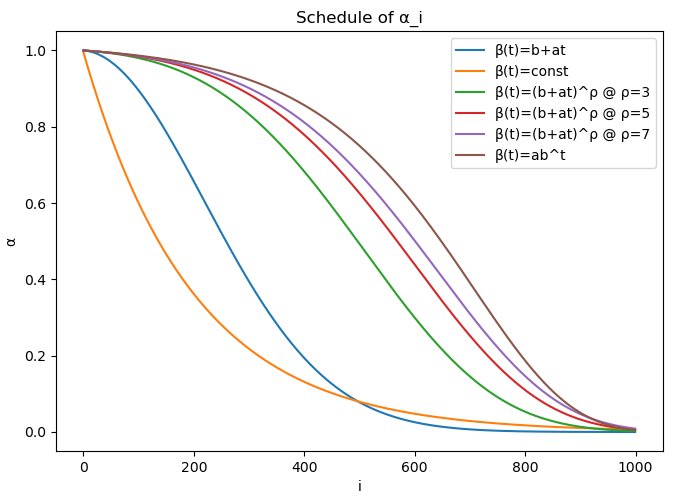
(a) DDPM

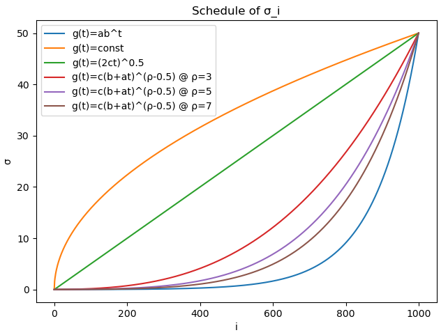
(b) NCSN

Figure 1: The schedules of $(\alpha_{i})$ for DDPM models and $(\sigma_{i})$ for NCSN (a.k.a. SMLD) models with different forward SDEs.

Sampling         We generate samples using the Euler-Maruyama solver for discretizing the reverse time SDEs, referred to as the predictor in [SSDK⁺21]. We set the number of discretized time steps $N=1000$, which follows [HJA20] and [SSDK⁺21].

Performance Metrics         The quality of the generated image samples is evaluated with Fréchet Inception Distance (FID, lower is better), which was first introduced by [HRU⁺17] for measuring the $2$-Wasserstein distance between the distributions of generated images with the distribution of real images. We also report the Inception Score (IS) (see [SGZ⁺16]) of the generated images as a secondary measure. However, IS (higher is better) only evaluates how realistic the generated images are without a comparison to real images. Each FID and IS measure is evaluated based on $20,000$ samples.

4.3 Empirical Results

Table 3 and Figures 2–3 show the performances of various diffusion models corresponding to different types of forward SDEs that we used. We have the following two important observations.

First, the experimental results are in good agreement with our theoretical prediction about the iteration complexity in Table 2. With the same number of discretized time steps, models (forward SDEs) with lower order of iteration complexity generally obtain a better FID score and IS (lower FID and higher IS) over training iterations. In addition, as predicted by the theory in Table 2, VE-SDE models generally perform worse than VP-SDEs. Among the VE-SDE models, the choice of $f\equiv 0$ and $g(t)=ab^{t}$ leads to the best performance in terms of FID and IS scores. We also remark that VE-SDE models can perform significantly better with a corrector (see [SSDK⁺21] for Predictor-Corrector sampling), and get close to the performance of VP-SDE models. However, our experimental results are based on the stochastic sampler without any corrector in order to fit the setup of our theory.

Second, our experimental results show that our proposed VP-SDE with a polynomial variance schedule $\beta(t)=(b+at)^{\rho}$ for some $\rho$ or an exponential variance schedule $\beta(t)=ab^{t}$ can outperform the other existing models, at least with simpler neural network architectures. The optimal $\rho$ is around $5$ according to Table 3. This is again consistent with our discussion in Section 3.1.

We also choose the best performing models from Table 3 and test the deeper neural network architecture in [SSDK⁺21] (which doubles the number of residual blocks per resolution, except for reduced batch size and reduced number of filters due to our memory limitation, as mentioned in Section 4.2). The results are shown in Figure 4 and Table 4. We can see that the performance of different models remains consistent in a more complex architecture setting.

Table 3: Performances of different SDE models on CIFAR-10 at 3,000,000 iterations

Model	FID$\downarrow$	IS$\uparrow$	References
DDPM (VP - $\beta(t)=\text{const}$)	17.46	8.19	[DBTHD21]
DDPM (VP - $\beta(t)=b+at$)	11.26	8.21	[HJA20]
DDPM (VP - $\beta(t)=(b+at)^{\rho},\rho=2$)	9.77	8.33
DDPM (VP - $\beta(t)=(b+at)^{\rho},\rho=3$)	9.67	8.32
DDPM (VP - $\beta(t)=(b+at)^{\rho},\rho=5$)	9.64	8.41	our paper
DDPM (VP - $\beta(t)=(b+at)^{\rho},\rho=7$)	10.22	8.41
DDPM (VP - $\beta(t)=(b+at)^{\rho},\rho=10$)	10.27	8.51
DDPM (VP - $\beta(t)=ab^{t}$)	9.98	8.39	our paper
NCSN (VE - $g(t)=ab^{t}$)	22.11	8.18	[SSDK+21]
NCSN (VE - $g(t)=\text{const}$)	461.42	1.18	[DBTHD21]
NCSN (VE - $g(t)=\sqrt{2at}$)	457.04	1.20	our paper
NCSN (VE - $g(t)=(b+at)^{\rho-\frac{1}{2}},\rho=2$)	369.51	1.34
NCSN (VE - $g(t)=(b+at)^{\rho-\frac{1}{2}},\rho=3$)	233.20	1.95
NCSN (VE - $g(t)=(b+at)^{\rho-\frac{1}{2}},\rho=5$)	137.55	4.01	our paper
NCSN (VE - $g(t)=(b+at)^{\rho-\frac{1}{2}},\rho=7$)	159.66	3.11
NCSN (VE - $g(t)=(b+at)^{\rho-\frac{1}{2}},\rho=10$)	99.89	4.91

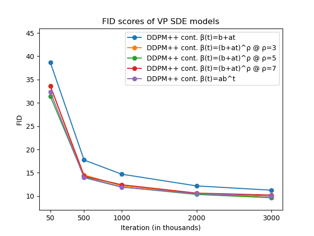
(a) DDPM

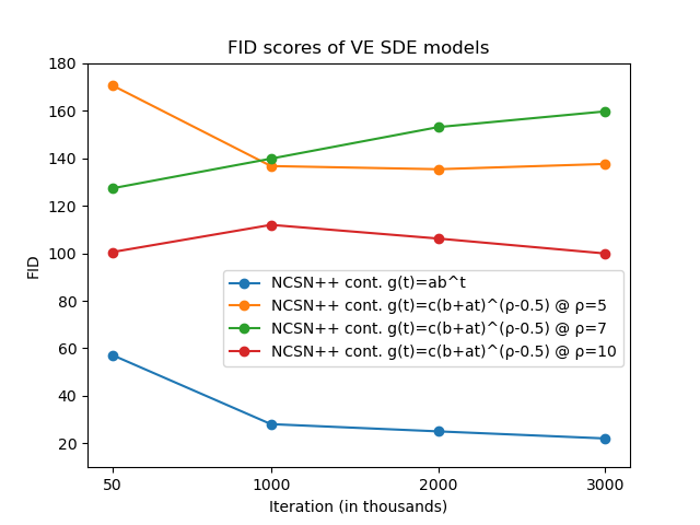
(b) NCSN (aka SMLD)

Figure 2: The FID score progressions of different SDE models on CIFAR-10

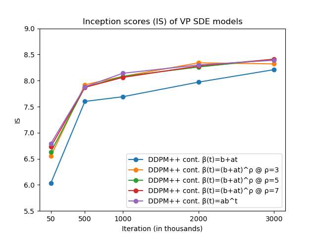
(a) DDPM

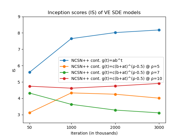
(b) NCSN (aka SMLD)

Figure 3: The inception score (IS) progressions of different SDE models on CIFAR-10

Table 4: Performances of deep versions of the best performing models from Table 3 on CIFAR-10 at 3,000,000 iterations. SMLD is also known as NCSN.

Model	FID$\downarrow$	IS$\uparrow$
DDPM deep (VP - $\beta(t)=b+at$)	9.22	8.25
DDPM deep (VP - $\beta(t)=(b+at)^{\rho},\rho=5$)	8.20	8.55
DDPM deep (VP - $\beta(t)=ab^{t}$)	8.14	8.44
NCSN deep (VE - $g(t)=ab^{t}$)	20.00	8.41

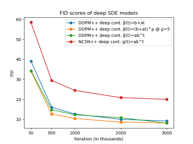
(a) FID

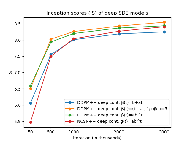
(b) IS

Figure 4: The FID and IS score progressions of the deep version of the best performing SDE models on CIFAR-10

5 Analysis: Proofs of the Main Results

5.1 Proof of Theorem 5

To prove Theorem 5, we study the three sources of errors discussed in Section 2 for convergence analysis: (1) the initialization of the algorithm at $\hat{p}_{T}$ instead of $p_{T}$, (2) the estimation error of the score function, and (3) the discretization error of the continuous-time process (2.7).

First, we study the error introduced due to the initialization at $\hat{p}_{T}$ instead of $p_{T}$. Recall the reverse SDE $\mathbf{z}_{t}$ given in (2.5):

$$d\mathbf{z}_{t}=\left[f(T-t)\mathbf{z}_{t}+(g(T-t))^{2}\nabla\log p_{T-t}(\mathbf{z}_{t})\right]dt+g(T-t)d\bar{\mathbf{B}}_{t},\quad\mathbf{z}_{0}\sim\hat{p}_{T}.$$ (5.1)

As discussed in Section 2, the distribution of $\mathbf{z}_{T}$ differs from $p_{0}$, because $\mathbf{z}_{0}\sim\hat{p}_{T}\neq p_{T}$. The following result provides a bound on $\mathcal{W}_{2}(\mathcal{L}(\mathbf{z}_{T}),p_{0}).$

Proposition 10.

Assume that $p_{0}$ is $m_{0}$-strongly-log-concave. Then, we have

$$\mathcal{W}_{2}(\mathcal{L}(\mathbf{z}_{T}),p_{0})\leq e^{-\int_{0}^{T}c(t)dt}\|\mathbf{x}_{0}\|_{L_{2}},$$ (5.2)

where $c(t)$ is given in (3.8).

The main challenge in analyzing the SDE $\mathbf{z}_{t}$ lies in studying the term $\nabla\log p_{T-t}(\mathbf{z}_{t})$. In general, this term is neither linear in $\mathbf{z}_{t}$ nor admits a closed-form expression. However, when $p_{0}$ is strongly log-concave, we are able to show that $\nabla_{\mathbf{x}}\log p_{T-t}(\mathbf{x})$ is also strongly log-concave. This fact, together with Itô’s formula for SDEs, allows us to establish Proposition 10. The proof of Propostion 10 is given in Section 5.1.1.

Now we consider the algorithm (• ‣ 2) with iterates $(\mathbf{y}_{k})$, and bound the errors due to score estimations and discretizations together. For any $k=0,1,2,\ldots,K$, $\mathbf{y}_{k}$ has the same distribution as $\hat{\mathbf{y}}_{k\eta}$, where $\hat{\mathbf{y}}_{t}$ is a continuous-time process with the dynamics:

$$d\hat{\mathbf{y}}_{t}=\left[f(T-t)\hat{\mathbf{y}}_{\lfloor t/\eta\rfloor\eta}+(g(T-t))^{2}s_{\theta}\left(\hat{\mathbf{y}}_{\lfloor t/\eta\rfloor\eta},T-\lfloor t/\eta\rfloor\eta\right)\right]dt+g(T-t)d\bar{\mathbf{B}}_{t},$$ (5.3)

with the initial distribution $\hat{\mathbf{y}}_{0}\sim\hat{p}_{T}$. We have the following result that provides an upper bound for $\|\mathbf{z}_{k\eta}-\hat{\mathbf{y}}_{k\eta}\|_{L_{2}}$ in terms of $\|\mathbf{z}_{(k-1)\eta}-\hat{\mathbf{y}}_{(k-1)\eta}\|_{L_{2}}$. This result plays a key role in the proof of Theorem 5.

Proposition 11.

Assume that $p_{0}$ is $m_{0}$-strongly-log-concave, i.e. $-\log p_{0}$ is $m_{0}$-strongly convex and $\nabla\log p_{0}$ is $L_{0}$-Lipschitz. For any $k=1,2,\ldots,K$,

$$\left\|\mathbf{z}_{k\eta}-\hat{\mathbf{y}}_{k\eta}\right\|_{L_{2}}$$

$$\leq\left(1-\int_{(k-1)\eta}^{k\eta}\mu(T-t)dt+M_{1}\eta\int_{(k-1)\eta}^{k\eta}(g(T-t))^{2}dt\right)\|\mathbf{z}_{(k-1)\eta}-\hat{\mathbf{y}}_{(k-1)\eta}\|_{L_{2}}$$

$$\qquad+M_{1}\eta\left(1+\|\mathbf{x}_{0}\|_{L_{2}}+c_{2}(T)\right)\int_{(k-1)\eta}^{k\eta}(g(T-t))^{2}dt+M\int_{(k-1)\eta}^{k\eta}(g(T-t))^{2}dt$$

$$\qquad\qquad+\sqrt{\eta}h_{k,\eta}\left(\int_{(k-1)\eta}^{k\eta}[f(T-t)+(g(T-t))^{2}L(T-t)]^{2}dt\right)^{1/2},$$ (5.4)

where $\mu(t)$, $0\leq t\leq T$, is defined in (3.10), $c_{2}(T)$ is defined in (3.13) and $h_{k,\eta}$ is given in (3.14).

We remark that the coefficient in front of the term $\left\|\mathbf{z}_{(k-1)\eta}-\hat{\mathbf{y}}_{(k-1)\eta}\right\|_{L_{2}}$ in (5.4) lies in between zero and one. Indeed, it follows from Assumption 4 and the definition of $\mu(t)$ in (3.10) that $\mu(t)\geq M_{1}\eta(g(t))^{2}$ for every $0\leq t\leq T$ and $\eta\max_{0\leq t\leq T}\mu(t)<1$ such that for any $j=1,2,\ldots,K$,

$$0\leq 1-\int_{(j-1)\eta}^{j\eta}\mu(T-t)dt+M_{1}\eta\int_{(j-1)\eta}^{j\eta}(g(T-t))^{2}dt\leq 1.$$

Now we are ready to prove Theorem 5.

Proof of Theorem 5.

Since $\hat{\mathbf{y}}_{k\eta}$ has the same distribution as $\mathbf{y}_{k}$, by applying (5.4), we have

$$\mathcal{W}_{2}(\mathcal{L}(\mathbf{z}_{K\eta}),\mathcal{L}(\mathbf{y}_{K}))$$

$$\leq\left\|\mathbf{z}_{K\eta}-\hat{\mathbf{y}}_{K\eta}\right\|_{L_{2}}$$

$$\leq\sum_{k=1}^{K}\prod_{j=k+1}^{K}\left(1-\int_{(j-1)\eta}^{j\eta}\mu(T-t)dt+M_{1}\eta\int_{(j-1)\eta}^{j\eta}(g(T-t))^{2}dt\right)$$

$$\qquad\cdot\Bigg{(}M_{1}\eta\left(1+\|\mathbf{x}_{0}\|_{L_{2}}+c_{2}(T)\right)\int_{(k-1)\eta}^{k\eta}(g(T-t))^{2}dt+M\int_{(k-1)\eta}^{k\eta}(g(T-t))^{2}dt$$

$$\qquad\qquad+\sqrt{\eta}h_{k,\eta}\left(\int_{(k-1)\eta}^{k\eta}\left[f(T-t)+(g(T-t))^{2}L(T-t)\right]^{2}dt\right)^{1/2}\Bigg{)}.$$

Moreover, we recall that $T=K\eta$ and by triangle inequality for $2$-Wasserstein distance,

$$\mathcal{W}_{2}(\mathcal{L}(\mathbf{y}_{K}),p_{0})\leq\mathcal{W}_{2}(\mathcal{L}(\mathbf{y}_{K}),\mathcal{L}(\mathbf{z}_{K\eta}))+\mathcal{W}_{2}(\mathcal{L}(\mathbf{z}_{K\eta}),p_{0}).$$

The proof is completed by applying Proposition 10. ∎

5.1.1 Proof of Proposition 10

Proof.

We recall that

$$d\tilde{\mathbf{x}}_{t}=\left[f(T-t)\tilde{\mathbf{x}}_{t}+(g(T-t))^{2}\nabla\log p_{T-t}(\tilde{\mathbf{x}}_{t})\right]dt+g(T-t)d\bar{\mathbf{B}}_{t},$$ (5.5)

with the initial distribution $\tilde{\mathbf{x}}_{0}\sim p_{T}$ and

$$d\mathbf{z}_{t}=\left[f(T-t)\mathbf{z}_{t}+(g(T-t))^{2}\nabla\log p_{T-t}(\mathbf{z}_{t})\right]dt+g(T-t)d\bar{\mathbf{B}}_{t},$$

with the initial distribution $\mathbf{z}_{0}\sim\hat{p}_{T}$. For the forward SDE (1.1), the transition density is Gaussian, and we have

$$p_{t}(\mathbf{x}_{t})=\int_{\mathbb{R}^{d}}p(\mathbf{x}_{t}|\mathbf{x}_{0})p_{0}(\mathbf{x}_{0})d\mathbf{x}_{0},$$

where

$$p(\mathbf{x}_{t}|\mathbf{x}_{0})=\frac{1}{\left(2\pi\int_{0}^{t}e^{-2\int_{s}^{t}f(v)dv}(g(s))^{2}ds\right)^{d/2}}\exp\left(-\frac{\|\mathbf{x}_{t}-e^{-\int_{0}^{t}f(s)ds}\mathbf{x}_{0}\|^{2}}{2\int_{0}^{t}e^{-2\int_{s}^{t}f(v)dv}(g(s))^{2}ds}\right).$$

This implies that

$$\log p_{T-t}(\mathbf{x}) =\log\int_{\mathbb{R}^{d}}\exp\left(-\frac{\|\mathbf{x}-e^{-\int_{0}^{T-t}f(s)ds}\mathbf{x}_{0}\|^{2}}{2\int_{0}^{T-t}e^{-2\int_{s}^{T-t}f(v)dv}(g(s))^{2}ds}\right)p_{0}(\mathbf{x}_{0})d\mathbf{x}_{0}$$

$$\qquad\qquad\qquad\qquad\qquad\qquad-\frac{d}{2}\log\left(2\pi\int_{0}^{t}e^{-2\int_{s}^{t}f(v)dv}(g(s))^{2}ds\right)$$

$$=\log\int_{\mathbb{R}^{d}}\exp\left(-\frac{\|\mathbf{x}-\mathbf{x}_{0}\|^{2}}{2\int_{0}^{T-t}e^{-2\int_{s}^{T-t}f(v)dv}(g(s))^{2}ds}\right)p_{0}\left(e^{\int_{0}^{T-t}f(s)ds}\mathbf{x}_{0}\right)d\mathbf{x}_{0}$$

$$\qquad\qquad\qquad\qquad+de^{\int_{0}^{T-t}f(s)ds}-\frac{d}{2}\log\left(2\pi\int_{0}^{t}e^{-2\int_{s}^{t}f(v)dv}(g(s))^{2}ds\right),$$

where we applied change-of-variable to obtain the last equation. Note that for any two functions $p,q:\mathbb{R}^{d}\rightarrow\mathbb{R}$, where $p$ is $m_{p}$-strongly-log-concave and $q$ is $m_{q}$-strongly-log-concave (i.e. $-\log p$ is $m_{p}$-strongly-convex and $-\log q$ is $m_{q}$-strongly-convex) then it is known that the convolution of $p$ and $q$, i.e. $\int_{\mathbb{R}^{d}}p(\mathbf{x}-\mathbf{y})q(\mathbf{y})d\mathbf{y}$ is $(m_{p}^{-1}+m_{q}^{-1})^{-1}$-strongly-log-concave; see e.g. Proposition 7.1 in [SW14]. It is easy to see that the function

$$\mathbf{x}\mapsto\exp\left(-\frac{\|\mathbf{x}\|^{2}}{2\int_{0}^{T-t}e^{-2\int_{s}^{T-t}f(v)dv}(g(s))^{2}ds}\right)$$

is $\frac{1}{\int_{0}^{T-t}e^{-2\int_{s}^{T-t}f(v)dv}(g(s))^{2}ds}$-strongly-log-concave, and the function

$$\mathbf{x}\mapsto p_{0}\left(e^{\int_{0}^{T-t}f(s)ds}\mathbf{x}\right)$$

is $m_{0}\left(e^{\int_{0}^{T-t}f(s)ds}\right)^{2}$-strongly-log-concave since we assumed that $\mathbf{x}\mapsto p_{0}(\mathbf{x})$ is $m_{0}$-strongly-log-concave. Hence, we conclude that $\log p_{T-t}(\mathbf{x})$ is $a(T-t)$-strongly-concave, where

$$a(T-t):=\frac{1}{\frac{1}{m_{0}}e^{-2\int_{0}^{T-t}f(s)ds}+\int_{0}^{T-t}e^{-2\int_{s}^{T-t}f(v)dv}(g(s))^{2}ds}.$$ (5.6)

Next, let us recall from (3.11) the definition of $m(T-t)$:

$$m(T-t):=2(g(T-t))^{2}a(T-t)-2f(T-t),\qquad 0\leq t\leq T,$$ (5.7)

where $a(T-t)$ is defined in (5.6). By Itô’s formula,

$$d\left(\|\tilde{\mathbf{x}}_{t}-\mathbf{z}_{t}\|^{2}e^{\int_{0}^{t}m(T-s)ds}\right)$$

$$=m(T-t)e^{\int_{0}^{t}m(T-s)ds}\|\tilde{\mathbf{x}}_{t}-\mathbf{z}_{t}\|^{2}dt+2e^{\int_{0}^{t}m(T-s)ds}\langle\tilde{\mathbf{x}}_{t}-\mathbf{z}_{t},d\tilde{\mathbf{x}}_{t}-d\mathbf{z}_{t}\rangle$$

$$=m(T-t)e^{\int_{0}^{t}m(T-s)ds}\|\tilde{\mathbf{x}}_{t}-\mathbf{z}_{t}\|^{2}dt+2e^{\int_{0}^{t}m(T-s)ds}\langle\tilde{\mathbf{x}}_{t}-\mathbf{z}_{t},f(T-t)(\tilde{\mathbf{x}}_{t}-\mathbf{z}_{t})\rangle dt$$

$$\qquad+2e^{\int_{0}^{t}m(T-s)ds}\left\langle\tilde{\mathbf{x}}_{t}-\mathbf{z}_{t},(g(T-t))^{2}\left(\nabla\log p_{T-t}(\tilde{\mathbf{x}}_{t})-\nabla\log p_{T-t}(\mathbf{z}_{t})\right)\right\rangle dt$$

$$\leq e^{\int_{0}^{t}m(T-s)ds}\left(m(T-t)+2f(T-t)-2(g(T-t))^{2}a(T-t)\right)\|\tilde{\mathbf{x}}_{t}-\mathbf{z}_{t}\|^{2}dt$$

$$=0.$$

This implies that

$$\|\tilde{\mathbf{x}}_{t}-\mathbf{z}_{t}\|^{2}e^{\int_{0}^{t}m(T-s)ds}\leq\|\tilde{\mathbf{x}}_{0}-\mathbf{z}_{0}\|^{2},$$ (5.8)

so that

$$\mathbb{E}\|\tilde{\mathbf{x}}_{T}-\mathbf{z}_{T}\|^{2}\leq e^{-\int_{0}^{T}m(T-s)ds}\mathbb{E}\|\tilde{\mathbf{x}}_{0}-\mathbf{z}_{0}\|^{2}.$$ (5.9)

Consider a coupling of $(\tilde{\mathbf{x}}_{0},\mathbf{z}_{0})$ such that $\tilde{\mathbf{x}}_{0}\sim p_{T}$, $\mathbf{z}_{0}\sim\hat{p}_{T}$ and $\mathbb{E}\|\tilde{\mathbf{x}}_{0}-\mathbf{z}_{0}\|^{2}=\mathcal{W}_{2}^{2}(p_{T},\hat{p}_{T})$. Together with (2.4), we conclude that

$$\mathcal{W}_{2}^{2}(\mathcal{L}(\mathbf{z}_{T}),p_{0}) =\mathcal{W}_{2}(\mathcal{L}(\mathbf{z}_{T}),\mathcal{L}(\tilde{\mathbf{x}}_{T}))\leq\mathbb{E}\|\tilde{\mathbf{x}}_{T}-\mathbf{z}_{T}\|^{2}$$

$$\leq e^{-\int_{0}^{T}m(T-s)ds}\mathcal{W}_{2}^{2}(p_{T},\hat{p}_{T})$$

$$\leq e^{-\int_{0}^{T}m(s)ds}e^{-2\int_{0}^{T}f(s)ds}\|\mathbf{x}_{0}\|_{L_{2}}^{2}=e^{-2\int_{0}^{T}c(t)dt}\|\mathbf{x}_{0}\|_{L_{2}}^{2},$$

where

$$c(t)=f(t)+\frac{m(t)}{2}=\frac{m_{0}(g(t))^{2}}{e^{-2\int_{0}^{t}f(s)ds}+m_{0}\int_{0}^{t}e^{-2\int_{s}^{t}f(v)dv}(g(s))^{2}ds},$$

and we have used (5.7). The proof is complete. ∎

5.1.2 Proof of Proposition 11

We first state a key technical lemma, which will be used in the proof of Proposition 11. The proof of the following result will be provided in Appendix A.1.

Lemma 12.

Suppose that Assumption 1 holds. Then, $\nabla_{\mathbf{x}}\log p_{T-t}(\mathbf{x})$ is $L(T-t)$-Lipschitz in $\mathbf{x}$, where $L(T-t)$ is given in (3.9).

Proof of Proposition 11.

First, we recall that

$$\mathbf{z}_{k\eta}=\mathbf{z}_{(k-1)\eta}+\int_{(k-1)\eta}^{k\eta}\left[f(T-t)\mathbf{z}_{t}+(g(T-t))^{2}\nabla\log p_{T-t}(\mathbf{z}_{t})\right]dt+\int_{(k-1)\eta}^{k\eta}g(T-t)d\bar{\mathbf{B}}_{t},$$

$$\hat{\mathbf{y}}_{k\eta}=\hat{\mathbf{y}}_{(k-1)\eta}+\int_{(k-1)\eta}^{k\eta}\left[f(T-t)\hat{\mathbf{y}}_{(k-1)\eta}+(g(T-t))^{2}s_{\theta}\left(\hat{\mathbf{y}}_{(k-1)\eta},T-(k-1)\eta\right)\right]dt$$

$$\qquad\qquad\qquad\qquad\qquad+\int_{(k-1)\eta}^{k\eta}g(T-t)d\bar{\mathbf{B}}_{t}.$$

It follows that

$$\mathbf{z}_{k\eta}-\hat{\mathbf{y}}_{k\eta}$$

$$=\mathbf{z}_{(k-1)\eta}-\hat{\mathbf{y}}_{(k-1)\eta}+\int_{(k-1)\eta}^{k\eta}f(T-t)\left(\mathbf{z}_{(k-1)\eta}-\hat{\mathbf{y}}_{(k-1)\eta}\right)dt$$

$$\qquad\qquad+\int_{(k-1)\eta}^{k\eta}(g(T-t))^{2}\left(\nabla\log p_{T-t}(\mathbf{z}_{(k-1)\eta})-\nabla\log p_{T-t}\left(\hat{\mathbf{y}}_{(k-1)\eta}\right)\right)dt$$

$$\qquad+\int_{(k-1)\eta}^{k\eta}\Big{[}f(T-t)(\mathbf{z}_{t}-\mathbf{z}_{(k-1)\eta})$$

$$\qquad\qquad\qquad\qquad\qquad+(g(T-t))^{2}\left(\nabla\log p_{T-t}(\mathbf{z}_{t})-\nabla\log p_{T-t}(\mathbf{z}_{(k-1)\eta})\right)\Big{]}dt$$

$$\qquad\qquad+\int_{(k-1)\eta}^{k\eta}(g(T-t))^{2}\left(\nabla\log p_{T-t}\left(\hat{\mathbf{y}}_{(k-1)\eta}\right)-s_{\theta}\left(\hat{\mathbf{y}}_{(k-1)\eta},T-(k-1)\eta\right)\right)dt.$$

This implies that

$$\left\|\mathbf{z}_{k\eta}-\hat{\mathbf{y}}_{k\eta}\right\|_{L_{2}}$$

$$\leq\Bigg{\|}\mathbf{z}_{(k-1)\eta}-\hat{\mathbf{y}}_{(k-1)\eta}+\int_{(k-1)\eta}^{k\eta}f(T-t)\left(\mathbf{z}_{(k-1)\eta}-\hat{\mathbf{y}}_{(k-1)\eta}\right)dt$$

$$\qquad\qquad+\int_{(k-1)\eta}^{k\eta}(g(T-t))^{2}\left(\nabla\log p_{T-t}(\mathbf{z}_{(k-1)\eta})-\nabla\log p_{T-t}\left(\hat{\mathbf{y}}_{(k-1)\eta}\right)\right)dt\Bigg{\|}_{L_{2}}$$

$$\quad+\Bigg{\|}\int_{(k-1)\eta}^{k\eta}\Big{[}f(T-t)(\mathbf{z}_{t}-\mathbf{z}_{(k-1)\eta})$$

$$\qquad\qquad\qquad\qquad\qquad\qquad+(g(T-t))^{2}\left(\nabla\log p_{T-t}(\mathbf{z}_{t})-\nabla\log p_{T-t}(\mathbf{z}_{(k-1)\eta})\right)\Big{]}dt\Bigg{\|}_{L_{2}}$$

$$\qquad\quad+\left\|\int_{(k-1)\eta}^{k\eta}(g(T-t))^{2}\left(\nabla\log p_{T-t}\left(\hat{\mathbf{y}}_{(k-1)\eta}\right)-s_{\theta}\left(\hat{\mathbf{y}}_{(k-1)\eta},T-(k-1)\eta\right)\right)dt\right\|_{L_{2}}.$$ (5.10)

Next, we provide upper bounds for the three terms in (5.10).

Bounding the first term in (5.10). We can compute that

$$\Bigg{\|}\mathbf{z}_{(k-1)\eta}-\hat{\mathbf{y}}_{(k-1)\eta}+\int_{(k-1)\eta}^{k\eta}f(T-t)\left(\mathbf{z}_{(k-1)\eta}-\hat{\mathbf{y}}_{(k-1)\eta}\right)dt$$

$$\qquad\qquad+\int_{(k-1)\eta}^{k\eta}(g(T-t))^{2}\left(\nabla\log p_{T-t}(\mathbf{z}_{(k-1)\eta})-\nabla\log p_{T-t}\left(\hat{\mathbf{y}}_{(k-1)\eta}\right)\right)dt\Bigg{\|}^{2}$$

$$=\left\|\mathbf{z}_{(k-1)\eta}-\hat{\mathbf{y}}_{(k-1)\eta}\right\|^{2}+\Bigg{\|}\int_{(k-1)\eta}^{k\eta}f(T-t)\left(\mathbf{z}_{(k-1)\eta}-\hat{\mathbf{y}}_{(k-1)\eta}\right)dt$$

$$\qquad\qquad+\int_{(k-1)\eta}^{k\eta}(g(T-t))^{2}\left(\nabla\log p_{T-t}(\mathbf{z}_{(k-1)\eta})-\nabla\log p_{T-t}\left(\hat{\mathbf{y}}_{(k-1)\eta}\right)\right)dt\Bigg{\|}^{2}$$

$$\qquad\qquad\qquad+2\int_{(k-1)\eta}^{k\eta}f(T-t)\left\|\mathbf{z}_{(k-1)\eta}-\hat{\mathbf{y}}_{(k-1)\eta}\right\|^{2}dt$$

$$+2\int_{(k-1)\eta}^{k\eta}\left\langle\mathbf{z}_{(k-1)\eta}-\hat{\mathbf{y}}_{(k-1)\eta},(g(T-t))^{2}\left(\nabla\log p_{T-t}(\mathbf{z}_{(k-1)\eta})-\nabla\log p_{T-t}\left(\hat{\mathbf{y}}_{(k-1)\eta}\right)\right)\right\rangle dt.$$

From the proof of Proposition 10, we know that $\log p_{T-t}(\mathbf{x})$ is $a(T-t)$-strongly-concave, where $a(T-t)$ is given in (5.6). Hence we have

$$\Bigg{\|}\mathbf{z}_{(k-1)\eta}-\hat{\mathbf{y}}_{(k-1)\eta}+\int_{(k-1)\eta}^{k\eta}f(T-t)\left(\mathbf{z}_{(k-1)\eta}-\hat{\mathbf{y}}_{(k-1)\eta}\right)dt$$

$$\qquad\qquad+\int_{(k-1)\eta}^{k\eta}(g(T-t))^{2}\left(\nabla\log p_{T-t}(\mathbf{z}_{(k-1)\eta})-\nabla\log p_{T-t}\left(\hat{\mathbf{y}}_{(k-1)\eta}\right)\right)dt\Bigg{\|}^{2}$$

$$\leq\left(1-\int_{(k-1)\eta}^{k\eta}m(T-t)dt\right)\left\|\mathbf{z}_{(k-1)\eta}-\hat{\mathbf{y}}_{(k-1)\eta}\right\|^{2}+\Bigg{(}\int_{(k-1)\eta}^{k\eta}f(T-t)\left\|\mathbf{z}_{(k-1)\eta}-\hat{\mathbf{y}}_{(k-1)\eta}\right\|dt$$

$$\qquad\qquad+\int_{(k-1)\eta}^{k\eta}(g(T-t))^{2}L(T-t)\left\|\mathbf{z}_{(k-1)\eta}-\hat{\mathbf{y}}_{(k-1)\eta}\right\|dt\Bigg{)}^{2}$$

$$\leq\left(1-\int_{(k-1)\eta}^{k\eta}m(T-t)dt+2\eta\int_{(k-1)\eta}^{k\eta}(f(T-t))^{2}dt+2\eta\int_{(k-1)\eta}^{k\eta}(g(T-t))^{4}(L(T-t))^{2}dt\right)$$

$$\qquad\qquad\cdot\left\|\mathbf{z}_{(k-1)\eta}-\hat{\mathbf{y}}_{(k-1)\eta}\right\|^{2},$$

where we applied Cauchy-Schwartz inequality and Lemma 12, and $m(T-t)$ is defined in (3.11) (also see (5.7)). Hence, we conclude that

$$\Bigg{\|}\mathbf{z}_{(k-1)\eta}-\hat{\mathbf{y}}_{(k-1)\eta}+\int_{(k-1)\eta}^{k\eta}f(T-t)\left(\mathbf{z}_{(k-1)\eta}-\hat{\mathbf{y}}_{(k-1)\eta}\right)dt$$

$$\qquad\qquad+\int_{(k-1)\eta}^{k\eta}(g(T-t))^{2}\left(\nabla\log p_{T-t}\left(\mathbf{z}_{(k-1)\eta}\right)-\nabla\log p_{T-t}\left(\hat{\mathbf{y}}_{(k-1)\eta}\right)\right)dt\Bigg{\|}_{L_{2}}$$

$$\leq\left(1-\int_{(k-1)\eta}^{k\eta}\mu(T-t)dt\right)\left\|\mathbf{z}_{(k-1)\eta}-\hat{\mathbf{y}}_{(k-1)\eta}\right\|_{L_{2}},$$ (5.11)

where we used the inequality $\sqrt{1-x}\leq 1-\frac{x}{2}$ for any $0\leq x\leq 1$ and the definition of $\mu(T-t)$ in (3.10) which can be rewritten as

$$\mu(T-t):=(g(T-t))^{2}a(T-t)-f(T-t)-\eta(f(T-t))^{2}-\eta(g(T-t))^{4}(L(T-t))^{2},\quad 0\leq t\leq T,$$

where $a(T-t)$ is given in (5.6).

Bounding the second term in (5.10). Using Lemma 12, we can compute that

$$\left\|\int_{(k-1)\eta}^{k\eta}\left[f(T-t)(\mathbf{z}_{t}-\mathbf{z}_{(k-1)\eta})+(g(T-t))^{2}\left(\nabla\log p_{T-t}(\mathbf{z}_{t})-\nabla\log p_{T-t}(\mathbf{z}_{(k-1)\eta})\right)\right]dt\right\|^{2}$$

$$\leq\left(\int_{(k-1)\eta}^{k\eta}[f(T-t)+(g(T-t))^{2}L(T-t)]\|\mathbf{z}_{t}-\mathbf{z}_{(k-1)\eta}\|dt\right)^{2}$$

$$\leq\eta\int_{(k-1)\eta}^{k\eta}[f(T-t)+(g(T-t))^{2}L(T-t)]^{2}\|\mathbf{z}_{t}-\mathbf{z}_{(k-1)\eta}\|^{2}dt,$$

which implies that

$$\left\|\int_{(k-1)\eta}^{k\eta}\left[f(T-t)(\mathbf{z}_{t}-\mathbf{z}_{(k-1)\eta})+(g(T-t))^{2}\left(\nabla\log p_{T-t}(\mathbf{z}_{t})-\nabla\log p_{T-t}\left(\mathbf{z}_{(k-1)\eta}\right)\right)\right]dt\right\|_{L_{2}}$$

$$\leq\left(\mathbb{E}\left[\eta\int_{(k-1)\eta}^{k\eta}[f(T-t)+(g(T-t))^{2}L(T-t)]^{2}\|\mathbf{z}_{t}-\mathbf{z}_{(k-1)\eta}\|^{2}dt\right]\right)^{1/2}$$

$$\leq\left(\eta\int_{(k-1)\eta}^{k\eta}[f(T-t)+(g(T-t))^{2}L(T-t)]^{2}dt\cdot\sup_{(k-1)\eta\leq t\leq k\eta}\mathbb{E}\|\mathbf{z}_{t}-\mathbf{z}_{(k-1)\eta}\|^{2}\right)^{1/2}$$

$$=\sqrt{\eta}\left(\int_{(k-1)\eta}^{k\eta}[f(T-t)+(g(T-t))^{2}L(T-t)]^{2}dt\right)^{1/2}\sup_{(k-1)\eta\leq t\leq k\eta}\left\|\mathbf{z}_{t}-\mathbf{z}_{(k-1)\eta}\right\|_{L_{2}}.$$ (5.12)

Bounding the third term in (5.10). We notice that

$$\left\|\int_{(k-1)\eta}^{k\eta}(g(T-t))^{2}\left(\nabla\log p_{T-t}(\hat{\mathbf{y}}_{(k-1)\eta})-s_{\theta}\left(\hat{\mathbf{y}}_{(k-1)\eta},T-(k-1)\eta\right)\right)dt\right\|_{L_{2}}$$

$$\leq\left\|\int_{(k-1)\eta}^{k\eta}(g(T-t))^{2}\left(\nabla\log p_{T-(k-1)\eta}(\hat{\mathbf{y}}_{(k-1)\eta})-s_{\theta}\left(\hat{\mathbf{y}}_{(k-1)\eta},T-(k-1)\eta\right)\right)dt\right\|_{L_{2}}$$

$$\qquad+\left\|\int_{(k-1)\eta}^{k\eta}(g(T-t))^{2}\left(\nabla\log p_{T-t}\left(\hat{\mathbf{y}}_{(k-1)\eta}\right)-\nabla\log p_{T-(k-1)\eta}\left(\hat{\mathbf{y}}_{(k-1)\eta}\right)\right)dt\right\|_{L_{2}}.$$

By Assumption 3, we have

$$\left\|\int_{(k-1)\eta}^{k\eta}(g(T-t))^{2}\left(\nabla\log p_{T-(k-1)\eta}(\hat{\mathbf{y}}_{(k-1)\eta})-s_{\theta}\left(\hat{\mathbf{y}}_{(k-1)\eta},T-(k-1)\eta\right)\right)dt\right\|_{L_{2}}$$

$$\leq M\int_{(k-1)\eta}^{k\eta}(g(T-t))^{2}dt.$$ (5.13)

Moreover, by Assumption 2, we have

$$\left\|\int_{(k-1)\eta}^{k\eta}(g(T-t))^{2}\left(\nabla\log p_{T-t}\left(\hat{\mathbf{y}}_{(k-1)\eta}\right)-\nabla\log p_{T-(k-1)\eta}\left(\hat{\mathbf{y}}_{(k-1)\eta}\right)\right)dt\right\|_{L_{2}}$$

$$\leq\int_{(k-1)\eta}^{k\eta}(g(T-t))^{2}\left\|\nabla\log p_{T-t}\left(\hat{\mathbf{y}}_{(k-1)\eta}\right)-\nabla\log p_{T-(k-1)\eta}\left(\hat{\mathbf{y}}_{(k-1)\eta}\right)\right\|_{L_{2}}dt$$

$$\leq\int_{(k-1)\eta}^{k\eta}(g(T-t))^{2}M_{1}\eta\left(1+\left\|\hat{\mathbf{y}}_{(k-1)\eta}\right\|_{L_{2}}\right)dt$$

$$\leq M_{1}\eta\left(1+\left\|\mathbf{z}_{(k-1)\eta}-\hat{\mathbf{y}}_{(k-1)\eta}\right\|_{L_{2}}+\|\mathbf{z}_{(k-1)\eta}\|_{L_{2}}\right)\int_{(k-1)\eta}^{k\eta}(g(T-t))^{2}dt.$$ (5.14)

Furthermore, we can compute that

$$\left\|\mathbf{z}_{(k-1)\eta}\right\|_{L_{2}}\leq\left\|\mathbf{z}_{(k-1)\eta}-\tilde{\mathbf{x}}_{(k-1)\eta}\right\|_{L_{2}}+\left\|\tilde{\mathbf{x}}_{(k-1)\eta}\right\|_{L_{2}},$$ (5.15)

where $\tilde{\mathbf{x}}_{t}$ is defined in (2.2). Moreover, by (5.8) in the proof of Proposition 10, we have

$$\left\|\mathbf{z}_{(k-1)\eta}-\tilde{\mathbf{x}}_{(k-1)\eta}\right\|_{L_{2}}\leq\left(\mathbb{E}\|\tilde{\mathbf{x}}_{0}-\mathbf{z}_{0}\|^{2}\right)^{1/2}=e^{-\int_{0}^{T}f(s)ds}\|\mathbf{x}_{0}\|_{L_{2}}\leq\|\mathbf{x}_{0}\|_{L_{2}},$$ (5.16)

where we applied (2.1) to obtain the equality in the above equation. Moreover, since $(\tilde{\mathbf{x}}_{t})_{0\leq t\leq T}$ is the time-reversal process of $(\mathbf{x}_{t})_{0\leq t\leq T}$, we have

$$\left\|\tilde{\mathbf{x}}_{(k-1)\eta}\right\|_{L_{2}}=\left\|\mathbf{x}_{T-(k-1)\eta}\right\|_{L_{2}}\leq\sup_{0\leq t\leq T}\|\mathbf{x}_{t}\|_{L_{2}}=:c_{2}(T).$$ (5.17)

Next, let us show that $c_{2}(T)$ can be computed as given by the formula in (3.13). By applying Itô’s formula to equation (2.1), we have

$$d\left(\|\mathbf{x}_{t}\|^{2}e^{2\int_{0}^{t}f(s)ds}\right) =2f(t)\|\mathbf{x}_{t}\|^{2}e^{2\int_{0}^{t}f(s)ds}dt$$

$$\qquad\qquad+2e^{2\int_{0}^{t}f(s)ds}\langle\mathbf{x}_{t},d\mathbf{x}_{t}\rangle+e^{2\int_{0}^{t}f(s)ds}\cdot d\cdot(g(t))^{2}dt.$$

By taking expectations, we obtain

$$d\left(\mathbb{E}\|\mathbf{x}_{t}\|^{2}e^{2\int_{0}^{t}f(s)ds}\right)=e^{2\int_{0}^{t}f(s)ds}\cdot d\cdot(g(t))^{2}dt,$$

which implies that

$$\mathbb{E}\|\mathbf{x}_{t}\|^{2} =e^{-2\int_{0}^{t}f(s)ds}\mathbb{E}\|\mathbf{x}_{0}\|^{2}+d\int_{0}^{t}e^{-2\int_{s}^{t}f(v)dv}(g(s))^{2}ds.$$ (5.18)

Therefore, we conclude that

$$c_{2}(T)=\sup_{0\leq t\leq T}\|\mathbf{x}_{t}\|_{L_{2}}=\sup_{0\leq t\leq T}\left(e^{-2\int_{0}^{t}f(s)ds}\|\mathbf{x}_{0}\|_{L_{2}}^{2}+d\int_{0}^{t}e^{-2\int_{s}^{t}f(v)dv}(g(s))^{2}ds\right)^{1/2}.$$ (5.19)

Therefore, by applying (5.14), (5.15), (5.16) and (5.17), we have

$$\left\|\int_{(k-1)\eta}^{k\eta}(g(T-t))^{2}\left(\nabla\log p_{T-t}\left(\hat{\mathbf{y}}_{(k-1)\eta}\right)-\nabla\log p_{T-(k-1)\eta}\left(\hat{\mathbf{y}}_{(k-1)\eta}\right)\right)dt\right\|_{L_{2}}$$

$$\leq M_{1}\eta\left\|\mathbf{z}_{(k-1)\eta}-\hat{\mathbf{y}}_{(k-1)\eta}\right\|_{L_{2}}\int_{(k-1)\eta}^{k\eta}(g(T-t))^{2}dt$$

$$\qquad\qquad\qquad+M_{1}\eta\left(1+\|\mathbf{x}_{0}\|_{L_{2}}+c_{2}(T)\right)\int_{(k-1)\eta}^{k\eta}(g(T-t))^{2}dt.$$

It follows that the third term in (5.10) is upper bounded by

$$M_{1}\eta\left\|\mathbf{z}_{(k-1)\eta}-\hat{\mathbf{y}}_{(k-1)\eta}\right\|_{L_{2}}\int_{(k-1)\eta}^{k\eta}(g(T-t))^{2}dt$$

$$\qquad+M_{1}\eta\left(1+\|\mathbf{x}_{0}\|_{L_{2}}+c_{2}(T)\right)\int_{(k-1)\eta}^{k\eta}(g(T-t))^{2}dt+M\int_{(k-1)\eta}^{k\eta}(g(T-t))^{2}dt.$$ (5.20)

Bounding (5.10). On combining (5.1.2), (5.1.2) and (5.1.2), we conclude that

$$\left\|\mathbf{z}_{k\eta}-\hat{\mathbf{y}}_{k\eta}\right\|_{L_{2}}^{2}$$

$$\leq\Bigg{\{}\left(1-\int_{(k-1)\eta}^{k\eta}\mu(T-t)dt+M_{1}\eta\int_{(k-1)\eta}^{k\eta}(g(T-t))^{2}dt\right)\left\|\mathbf{z}_{(k-1)\eta}-\hat{\mathbf{y}}_{(k-1)\eta}\right\|_{L_{2}}$$

$$\quad+M_{1}\eta\left(1+\|\mathbf{x}_{0}\|_{L_{2}}+c_{2}(T)\right)\int_{(k-1)\eta}^{k\eta}(g(T-t))^{2}dt+M\int_{(k-1)\eta}^{k\eta}(g(T-t))^{2}dt$$

$$\qquad+\sqrt{\eta}\left(\int_{(k-1)\eta}^{k\eta}[f(T-t)+(g(T-t))^{2}L(T-t)]^{2}dt\right)^{1/2}\sup_{(k-1)\eta\leq t\leq k\eta}\|\mathbf{z}_{t}-\mathbf{z}_{(k-1)\eta}\|_{L_{2}}\Bigg{\}}^{2}.$$ (5.21)

We need one more result, which provides an upper bound for $\sup_{(k-1)\eta\leq t\leq k\eta}\|\mathbf{z}_{t}-\mathbf{z}_{(k-1)\eta}\|_{L_{2}}$. The proof of Lemma 13 is given in Appendix A.2.

Lemma 13.

For any $k=1,2,\ldots,K$,

$$\sup_{(k-1)\eta\leq t\leq k\eta}\left\|\mathbf{z}_{t}-\mathbf{z}_{(k-1)\eta}\right\|_{L_{2}} \leq c_{1}(T)\int_{(k-1)\eta}^{k\eta}\left[f(T-s)+(g(T-s))^{2}L(T-s)\right]ds$$

$$\quad+c_{2}(T)\int_{T-k\eta}^{T-(k-1)\eta}f(s)ds+\left(\int_{T-k\eta}^{T-(k-1)\eta}(g(s))^{2}ds\right)^{1/2}\sqrt{d},$$

where we recall from (3.12)-(3.13) that

$$c_{1}(T):=\sup_{0\leq t\leq T}e^{-\frac{1}{2}\int_{0}^{t}m(T-s)ds}e^{-\int_{0}^{T}f(s)ds}\|\mathbf{x}_{0}\|_{L_{2}},$$

$$c_{2}(T):=\sup_{0\leq t\leq T}\left(e^{-2\int_{0}^{t}f(s)ds}\|\mathbf{x}_{0}\|_{L_{2}}^{2}+d\int_{0}^{t}e^{-2\int_{s}^{t}f(v)dv}(g(s))^{2}ds\right)^{1/2}.$$

By applying Lemma 13, we conclude from (5.1.2) that

$$\left\|\mathbf{z}_{k\eta}-\hat{\mathbf{y}}_{k\eta}\right\|_{L_{2}}^{2}$$

$$\leq\Bigg{\{}\left(1-\int_{(k-1)\eta}^{k\eta}\mu(T-t)dt+M_{1}\eta\int_{(k-1)\eta}^{k\eta}(g(T-t))^{2}dt\right)\left\|\mathbf{z}_{(k-1)\eta}-\hat{\mathbf{y}}_{(k-1)\eta}\right\|_{L_{2}}$$

$$\qquad+M_{1}\eta\left(1+\|\mathbf{x}_{0}\|_{L_{2}}+c_{2}(T)\right)\int_{(k-1)\eta}^{k\eta}(g(T-t))^{2}dt+M\int_{(k-1)\eta}^{k\eta}(g(T-t))^{2}dt$$

$$\qquad\qquad+\sqrt{\eta}h_{k,\eta}\left(\int_{(k-1)\eta}^{k\eta}[f(T-t)+(g(T-t))^{2}L(T-t)]^{2}dt\right)^{1/2}\Bigg{\}}^{2},$$

where $h_{k,\eta}$ is defined in (3.14). The proof of Proposition 11 is hence complete. ∎

5.2 Proof of Proposition 6

Proof of Proposition 6.

The proof of Proposition 6 will be postponed to Appendix B.2. ∎

5.3 Proof of Proposition 7

Proof of Proposition 7.

By the definition of $h_{k,\eta}$ in (3.14), we have

$$h_{k,\eta}\geq\min_{0\leq t\leq T}g(t)\sqrt{\eta}\sqrt{d}.$$

Therefore, we have

RHS of (3.15)

$$\geq e^{-\int_{0}^{K\eta}c(t)dt}\|\mathbf{x}_{0}\|_{L_{2}}+\sum_{k=1}^{K}\prod_{j=k+1}^{K}\left(1-\int_{(j-1)\eta}^{j\eta}\mu(T-t)dt\right)$$

$$\quad\cdot\left(M\int_{(k-1)\eta}^{k\eta}(g(T-t))^{2}dt+\sqrt{\eta}h_{k,\eta}\left(\int_{(k-1)\eta}^{k\eta}[f(T-t)+(g(T-t))^{2}L(T-t)]^{2}dt\right)^{1/2}\right)$$

$$\geq e^{-\int_{0}^{K\eta}c(t)dt}\|\mathbf{x}_{0}\|_{L_{2}}$$

$$\qquad+\sum_{k=1}^{K}\left(1-\eta\max_{0\leq t\leq T}\mu(t)\right)^{K-k}\left(\sqrt{\eta}\min_{0\leq T}g(t)\sqrt{\eta}\sqrt{d}\sqrt{\eta}\min_{0\leq t\leq T}\left(f(t)+(g(t))^{2}L(t)\right)\right)$$

$$=e^{-\int_{0}^{K\eta}c(t)dt}\|\mathbf{x}_{0}\|_{L_{2}}$$

$$\qquad\qquad+\sqrt{\eta}\sqrt{d}\frac{1-\left(1-\eta\max_{0\leq t\leq T}\mu(t)\right)^{K}}{\max_{0\leq t\leq T}\mu(t)}\left(\min_{0\leq t\leq T}g(t)\min_{0\leq t\leq T}\left(f(t)+(g(t))^{2}L(t)\right)\right)$$

$$\geq e^{-\int_{0}^{K\eta}c(t)dt}\|\mathbf{x}_{0}\|_{L_{2}}$$

$$\qquad\qquad+\sqrt{\eta}\sqrt{d}\frac{1-e^{-K\eta\max_{0\leq t\leq T}\mu(t)}}{\max_{0\leq t\leq T}\mu(t)}\left(\min_{0\leq t\leq T}g(t)\min_{0\leq t\leq T}\left(f(t)+(g(t))^{2}L(t)\right)\right),$$

where the equality above is due to the formula for the finite sum of a geometric series and we used the inequality that $1-x\leq e^{-x}$ for any $0\leq x\leq 1$ to obtain the last inequality above. Therefore, in order for $\text{RHS of \eqref{main:thm:upper:bound}}\leq\epsilon$, we must have

$$e^{-\int_{0}^{K\eta}c(t)dt}\|\mathbf{x}_{0}\|_{L_{2}}\leq\epsilon,$$

which implies that $K\eta\rightarrow\infty$ as $\epsilon\rightarrow 0$ and in particular

$$T=K\eta=\Omega(1),$$ (5.22)

(since under our assumptions on $f$ and $g$, $c(t)$ which is defined in (3.8) is positive and continuous so that $\int_{0}^{t}c(s)ds$ is finite for any $t\in(0,\infty)$ and strictly increasing from $0$ to $\infty$ as $t$ increases from $0$ to $\infty$), and we also need

$$\sqrt{\eta}\sqrt{d}\frac{1-e^{-K\eta\max_{0\leq t\leq T}\mu(t)}}{\max_{0\leq t\leq T}\mu(t)}\left(\min_{0\leq t\leq T}g(t)\min_{0\leq t\leq T}\left(f(t)+(g(t))^{2}L(t)\right)\right)\leq\epsilon.$$ (5.23)

Note that by the definition of $\mu(t)$ in (3.11) and $c(t)$ in (3.8), we have $\max_{0\leq t\leq T}\mu(t)\leq\max_{0\leq t\leq T}c(t)=\max_{0\leq t\leq K\eta}c(t)$. Together with $e^{-\int_{0}^{K\eta}c(t)dt}=\mathcal{O}(\epsilon/\sqrt{d})$ (since $\|\mathbf{x}_{0}\|_{L_{2}}\leq\mathcal{O}(\sqrt{d})$ from (3.1)) and the assumption that $\max_{0\leq s\leq t}c(s)\leq c_{1}\left(\int_{0}^{t}c(s)ds\right)^{\rho}+c_{2}$ uniformly in $t$ for some $c_{1},c_{2},\rho>0$, it is easy to see that $\max_{0\leq t\leq K\eta}c(t)=\mathcal{O}\left(\left(\log\left(\sqrt{d}/\epsilon\right)\right)^{\rho}\right)$ and hence $\max_{0\leq t\leq T}\mu(t)=\mathcal{O}\left(\left(\log\left(\sqrt{d}/\epsilon\right)\right)^{\rho}\right)$. Moreover, under our assumption $\mu(t)\geq\frac{1}{4}m(t)$ for any $0\leq t\leq T$, where $\mu(t),m(t)$ are defined in (3.10) and (3.11) and since we assumed $\min_{t\geq 0}g(t)>0$, we have $m(t)>0$ for any $t$. Together with $T=K\eta=\Omega(1)$ from (5.22), we have $\max_{0\leq t\leq T}\mu(t)\geq\Omega(1)$. Since $K\eta\rightarrow\infty$ as $\epsilon\rightarrow 0$, we have $1-e^{-K\eta\max_{0\leq t\leq T}\mu(t)}=\Omega(1)$. Therefore, it follows from (5.23) that $\eta=\widetilde{\mathcal{O}}\left(\frac{\epsilon^{2}}{d}\right)$, where $\widetilde{\mathcal{O}}$ ignores the logarithmic dependence on $\epsilon$ and $d$ and we used the assumptions that $\min_{t\geq 0}g(t)>0$ and $\min_{t\geq 0}(f(t)+(g(t))^{2}L(t))>0$. Hence, we conclude that we have the following lower bound for the complexity: $K=\widetilde{\Omega}\left(\frac{d}{\epsilon^{2}}\right),$ where $\widetilde{\Omega}$ ignores the logarithmic dependence on $\epsilon$ and $d$. This completes the proof. ∎

5.4 Proof of Proposition 8

Proof of Proposition 8.

When $\mathbf{x}_{0}\sim\mathcal{N}(0,\sigma_{0}^{2}I_{d})$, we can compute that

$$\nabla_{\mathbf{x}}\log p_{T-t}(\mathbf{x}) =\nabla_{\mathbf{x}}\log\int_{\mathbb{R}^{d}}\exp\left(-\frac{\|\mathbf{x}-e^{-\int_{0}^{T-t}f(s)ds}\mathbf{x}_{0}\|^{2}}{2\int_{0}^{T-t}e^{-2\int_{s}^{T-t}f(v)dv}(g(s))^{2}ds}\right)p_{0}(\mathbf{x}_{0})d\mathbf{x}_{0}$$

$$=\nabla_{\mathbf{x}}\log\int_{\mathbb{R}^{d}}\exp\left(-\frac{\|\mathbf{x}-e^{-\int_{0}^{T-t}f(s)ds}\mathbf{x}_{0}\|^{2}}{2\int_{0}^{T-t}e^{-2\int_{s}^{T-t}f(v)dv}(g(s))^{2}ds}\right)\exp\left(-\frac{\|\mathbf{x}_{0}\|^{2}}{2\sigma_{0}^{2}}\right)d\mathbf{x}_{0}$$

$$=\nabla_{\mathbf{x}}\log\int_{\mathbb{R}^{d}}\exp\left(-\frac{\|((a(T-t))^{2}\sigma_{0}^{2}+b(T-t))\mathbf{x}_{0}-a(T-t)\sigma_{0}^{2}\mathbf{x}\|^{2}}{2b(T-t)\sigma_{0}^{2}((a(T-t))^{2}\sigma_{0}^{2}+b(T-t))}\right)$$

$$\qquad\qquad\qquad\qquad\qquad\qquad\cdot\exp\left(-\frac{\|\mathbf{x}\|^{2}}{2((a(T-t))^{2}\sigma_{0}^{2}+b(T-t))}\right)d\mathbf{x}_{0}$$

$$=-\frac{1}{(a_{1}(T-t))^{2}\sigma_{0}^{2}+a_{2}(T-t)}\mathbf{x},$$

where

$$a_{1}(T-t):=e^{-\int_{0}^{T-t}f(s)ds},\qquad a_{2}(T-t):=\int_{0}^{T-t}e^{-2\int_{s}^{T-t}f(v)dv}(g(s))^{2}ds.$$ (5.24)

Therefore, under the assumption $\mathbf{x}_{0}\sim\mathcal{N}(0,\sigma_{0}^{2}I_{d})$, the discretization of (2.5) is given by:

$$\mathbf{y}_{k}=\left(1-\int_{(k-1)\eta}^{k\eta}\alpha(T-t)dt\right)\mathbf{y}_{k-1}+\left(\int_{(k-1)\eta}^{k\eta}(g(T-t))^{2}dt\right)^{1/2}\xi_{k},$$ (5.25)

where

$$\alpha(T-t):=\frac{(g(T-t))^{2}}{(a_{1}(T-t))^{2}\sigma_{0}^{2}+a_{2}(T-t)}-f(T-t),$$ (5.26)

where $a_{1}(T-t)$ and $a_{2}(T-t)$ are defined in (5.24), and $\xi_{k}$ are i.i.d. Gaussian random vectors $\mathcal{N}(0,I_{d})$ and $\mathbf{y}_{0}$ follows the same distribution as $\hat{p}_{T}$ in (2.3).

Since $\mathbf{y}_{K}$ and $\mathbf{x}_{0}$ are both mean zero Gaussian random vectors, by using the explicit formula for the $\mathcal{W}_{2}$ distance between two Gaussian distributions, we have

$$\mathcal{W}_{2}\left(\mathcal{L}(\mathbf{y}_{K}),\mathcal{L}(\mathbf{x}_{0})\right)=\left(\text{Tr}\left(\Sigma_{K}+\sigma_{0}^{2}I_{d}-2\left(\Sigma_{K}^{1/2}\sigma_{0}^{2}I_{d}\Sigma_{K}^{1/2}\right)^{1/2}\right)\right)^{1/2},$$

where

$$\Sigma_{k}=\mathbb{E}\left[\mathbf{y}_{k}\mathbf{y}_{k}^{\top}\right],\qquad k=0,1,\ldots,K,$$

is the covariance matrix of $\mathbf{y}_{k}$.

It is easy to compute that for any $k=1,2,\ldots,K$,

$$\Sigma_{k}=\left(1-\int_{(k-1)\eta}^{k\eta}\alpha(T-t)dt\right)^{2}\Sigma_{k-1}+\int_{(k-1)\eta}^{k\eta}(g(T-t))^{2}dt\cdot I_{d},$$

where $\alpha(T-t)$ is defined in (5.26) with

$$\Sigma_{0}=\int_{0}^{T}e^{-2\int_{s}^{T}f(v)dv}(g(s))^{2}ds\cdot I_{d}.$$

Therefore, one can deduce that

$$\Sigma_{k}=\hat{\sigma}_{k}^{2}I_{d},\qquad k=0,1,\ldots,K,$$ (5.27)

where

$$\hat{\sigma}_{k}^{2}=\left(1-\int_{(k-1)\eta}^{k\eta}\alpha(T-t)dt\right)^{2}\hat{\sigma}_{k-1}^{2}+\int_{(k-1)\eta}^{k\eta}(g(T-t))^{2}dt,$$ (5.28)

with

$$\hat{\sigma}_{0}^{2}=\int_{0}^{T}e^{-2\int_{s}^{T}f(v)dv}(g(s))^{2}ds.$$ (5.29)

Moreover, we get

$$\mathcal{W}_{2}\left(\mathcal{L}(\mathbf{y}_{K}),\mathcal{L}(\mathbf{x}_{0})\right)=\left(\text{Tr}\left(\hat{\sigma}_{K}^{2}I_{d}+\sigma_{0}^{2}I_{d}-2\left(\hat{\sigma}_{K}\sigma_{0}^{2}\hat{\sigma}_{K}\right)^{1/2}I_{d}\right)\right)^{1/2}=\sqrt{d}\left|\hat{\sigma}_{K}-\sigma_{0}\right|.$$ (5.30)

One can easily compute from (5.28) and (5.29) that

$$\hat{\sigma}_{K}^{2} =\sum_{j=1}^{K}\prod_{i=j+1}^{K}\left(1-\int_{(i-1)\eta}^{i\eta}\alpha(T-t)dt\right)^{2}\int_{(j-1)\eta}^{j\eta}(g(T-t))^{2}dt$$

$$\qquad\qquad\qquad+\prod_{i=1}^{K}\left(1-\int_{(i-1)\eta}^{i\eta}\alpha(T-t)dt\right)^{2}\int_{0}^{T}e^{-2\int_{s}^{T}f(v)dv}(g(s))^{2}ds,$$ (5.31)

where $\alpha(T-t)$ is defined in (5.26).

By discrete approximation of a Riemann integral, with fixed $K\eta=T$, we have

$$\left|\hat{\sigma}_{K}^{2}-\int_{0}^{T}e^{-2\int_{t}^{T}\alpha(T-s)ds}(g(T-t))^{2}dt-e^{-2\int_{0}^{T}\alpha(s)ds}\int_{0}^{T}e^{-2\int_{s}^{T}f(v)dv}(g(s))^{2}ds\right|=\Theta(\eta),$$

as $\eta\rightarrow 0$. Indeed, one can show that there exists some $c_{0}\in\mathbb{R}$, such that

$$\hat{\sigma}_{K}^{2}=\int_{0}^{T}e^{-2\int_{t}^{T}\alpha(T-s)ds}(g(T-t))^{2}dt+e^{-2\int_{0}^{T}\alpha(s)ds}\int_{0}^{T}e^{-2\int_{s}^{T}f(v)dv}(g(s))^{2}ds+c_{0}\eta+\mathcal{O}(\eta^{2}),$$ (5.32)

as $\eta\rightarrow 0$. Next, let us show that (5.32) holds as well as spell out the constant $c_{0}$ explicitly.

First, we can compute that

$$\log\prod_{i=1}^{K}\left(1-\int_{(i-1)\eta}^{i\eta}\alpha(T-t)dt\right)^{2}$$

$$=2\sum_{i=1}^{K}\log\left(1-\int_{(i-1)\eta}^{i\eta}\alpha(T-t)dt\right)$$

$$=2\sum_{i=1}^{K}\left(-\int_{(i-1)\eta}^{i\eta}\alpha(T-t)dt-\frac{1}{2}\left(\int_{(i-1)\eta}^{i\eta}\alpha(T-t)dt\right)^{2}+\mathcal{O}(\eta^{3})\right),$$

which implies that

$$\log\prod_{i=1}^{K}\left(1-\int_{(i-1)\eta}^{i\eta}\alpha(T-t)dt\right)^{2}-\log\left(e^{-2\int_{0}^{T}\alpha(T-t)dt}\right)$$

$$=-\sum_{i=1}^{K}\left(\int_{(i-1)\eta}^{i\eta}\alpha(T-t)dt\right)^{2}+\mathcal{O}(\eta^{2})$$

$$=-\eta\int_{0}^{T}(\alpha(T-t))^{2}dt+\mathcal{O}(\eta^{2}).$$

Therefore, we have

$$\prod_{i=1}^{K}\left(1-\int_{(i-1)\eta}^{i\eta}\alpha(T-t)dt\right)^{2}$$

$$=e^{-2\int_{0}^{T}\alpha(s)ds}e^{\log\prod_{i=1}^{K}\left(1-\int_{(i-1)\eta}^{i\eta}\alpha(T-t)dt\right)^{2}-\log\left(e^{-2\int_{0}^{T}\alpha(T-t)dt}\right)}$$

$$=e^{-2\int_{0}^{T}\alpha(s)ds}\left(1-\eta\int_{0}^{T}(\alpha(T-t))^{2}dt+\mathcal{O}(\eta^{2})\right).$$

Similarly, we can show that

$$\sum_{j=1}^{K}\prod_{i=j+1}^{K}\left(1-\int_{(i-1)\eta}^{i\eta}\alpha(T-t)dt\right)^{2}\int_{(j-1)\eta}^{j\eta}(g(T-t))^{2}dt$$

$$=\sum_{j=1}^{K}e^{-2\int_{j\eta}^{K\eta}\alpha(T-t)dt}\int_{(j-1)\eta}^{j\eta}(g(T-t))^{2}dt$$

$$\qquad\qquad\qquad-\eta\sum_{j=1}^{K}e^{-2\int_{j\eta}^{K\eta}\alpha(T-t)dt}\int_{j\eta}^{K\eta}(\alpha(T-t))^{2}dt\int_{(j-1)\eta}^{j\eta}(g(T-t))^{2}dt+\mathcal{O}(\eta^{2})$$

$$=\sum_{j=1}^{K}\int_{(j-1)\eta}^{j\eta}e^{-2\int_{j\eta}^{K\eta}\alpha(T-s)ds}(g(T-t))^{2}dt$$

$$\qquad\qquad-\eta\int_{0}^{T}e^{-2\int_{t}^{T}\alpha(T-s)ds}\left(\int_{t}^{T}(\alpha(T-s))^{2}ds\right)(g(T-t))^{2}dt+\mathcal{O}(\eta^{2}).$$

Moreover,

$$\sum_{j=1}^{K}\int_{(j-1)\eta}^{j\eta}e^{-2\int_{j\eta}^{K\eta}\alpha(T-s)ds}(g(T-t))^{2}dt$$

$$=\sum_{j=1}^{K}\int_{(j-1)\eta}^{j\eta}e^{-2\int_{t}^{K\eta}\alpha(T-s)ds}\left(1-2\int_{j\eta}^{t}\alpha(T-s)ds+\mathcal{O}(\eta^{2})\right)(g(T-t))^{2}dt$$

$$=\int_{0}^{T}e^{-2\int_{t}^{T}\alpha(T-s)ds}(g(T-t))^{2}dt$$

$$\qquad\qquad\qquad+\eta\int_{0}^{T}e^{-2\int_{t}^{T}\alpha(T-s)ds}\alpha(T-t)(g(T-t))^{2}dt+\mathcal{O}(\eta^{2}).$$

Hence, we conclude that (5.32) holds with

$$c_{0} :=-e^{-2\int_{0}^{T}\alpha(s)ds}\int_{0}^{T}(\alpha(T-t))^{2}dt\int_{0}^{T}e^{-2\int_{s}^{T}f(v)dv}(g(s))^{2}ds$$

$$\qquad\qquad-\int_{0}^{T}e^{-2\int_{t}^{T}\alpha(T-s)ds}\left(\int_{t}^{T}(\alpha(T-s))^{2}ds\right)(g(T-t))^{2}dt$$

$$\qquad\qquad\qquad\qquad+\int_{0}^{T}e^{-2\int_{t}^{T}\alpha(T-s)ds}\alpha(T-t)(g(T-t))^{2}dt,$$ (5.33)

which can be rewritten as

$$c_{0} =-e^{-2\int_{0}^{T}\alpha(s)ds}\int_{0}^{T}(\alpha(t))^{2}dt\int_{0}^{T}e^{-2\int_{s}^{T}f(v)dv}(g(s))^{2}ds$$

$$\qquad-\int_{0}^{T}e^{-2\int_{0}^{t}\alpha(s)ds}\left(\int_{0}^{t}(\alpha(s))^{2}ds\right)(g(t))^{2}dt+\int_{0}^{T}e^{-2\int_{0}^{t}\alpha(s)ds}\alpha(t)(g(t))^{2}dt,$$ (5.34)

where we recall that $\alpha(t)$ defined in (5.26). We assume that $f,g$ are given such that

$$c_{0}=\Theta(1),\qquad\text{as $T\rightarrow\infty$}.$$ (5.35)

Assumption (5.35) is a mild assumption on $f,g$. See the discussion in Remark 14 at the end of this section.

On the other hand, $\tilde{\mathbf{x}}_{T-t}$ has the same distribution as $\mathbf{x}_{t}$ for any $0\leq t\leq T$, where

$$d\tilde{\mathbf{x}}_{t}=-\alpha(T-t)\tilde{\mathbf{x}}_{t}dt+g(T-t)d\bar{\mathbf{B}}_{t},$$

with $\tilde{\mathbf{x}}_{0}\sim p_{T}$ such that

$$\tilde{\mathbf{x}}_{0}=e^{-\int_{0}^{T}f(s)ds}\mathbf{x}_{0}+\int_{0}^{T}e^{-\int_{s}^{T}f(v)dv}g(s)d\mathbf{B}_{s}.$$

Since $\tilde{\mathbf{x}}_{T}$ has the same distribution as $\mathbf{x}_{0}$, their covariance matrices are the same such that

$$\mathbb{E}\left[\tilde{\mathbf{x}}_{T}\tilde{\mathbf{x}}_{T}^{\top}\right] =\int_{0}^{T}e^{-2\int_{t}^{T}\alpha(T-s)ds}(g(T-t))^{2}dt\cdot I_{d}$$

$$\qquad\qquad+e^{-2\int_{0}^{T}\alpha(s)ds}\left(e^{-2\int_{0}^{T}f(s)ds}\sigma_{0}^{2}+\int_{0}^{T}e^{-2\int_{s}^{T}f(v)dv}(g(s))^{2}ds\right)\cdot I_{d}$$

$$=\mathbb{E}\left[\mathbf{x}_{0}\mathbf{x}_{0}^{\top}\right]=\sigma_{0}^{2}I_{d},$$

This implies that

$$\hat{\sigma}_{K}^{2}=\sigma_{0}^{2}-e^{-2\int_{0}^{T}\alpha(s)ds}e^{-2\int_{0}^{T}f(s)ds}\sigma_{0}^{2}+c_{0}\eta+\mathcal{O}(\eta^{2}),$$ (5.36)

where $\alpha(\cdot)$ is defined in (5.26) and $c_{0}$ is given in (5.34), and by the definition of $\alpha(\cdot)$, we can equivalently write (5.36) as

$$\hat{\sigma}_{K}^{2}=\sigma_{0}^{2}-e^{-2\int_{0}^{T}\gamma(s)ds}\sigma_{0}^{2}+c_{0}\eta+\mathcal{O}(\eta^{2}),$$ (5.37)

where

$$\gamma(t):=\frac{(g(t))^{2}}{(a_{1}(t))^{2}\sigma_{0}^{2}+a_{2}(t)},$$ (5.38)

with $a_{1}(\cdot),a_{2}(\cdot)$ defined in (5.24).

If there exists some $T=T(\epsilon)$ and $\bar{\eta}=\bar{\eta}(\epsilon)$ such that $\mathcal{W}_{2}(\mathcal{L}(\mathbf{y}_{K}),p_{0})\leq\epsilon$ for any $K\geq\bar{K}:=T/\bar{\eta}$ (with $\eta=T/K\leq\bar{\eta}$) then we must have

$$\mathcal{W}_{2}\left(\mathcal{L}(\mathbf{y}_{K}),\mathcal{L}(\mathbf{x}_{0})\right)=\sqrt{d}\left|\hat{\sigma}_{K}-\sigma_{0}\right|\leq\epsilon,$$

for any $K\geq\bar{K}:=T/\bar{\eta}$ so that

$$\left|\hat{\sigma}_{K}^{2}-\sigma_{0}^{2}\right|=|\hat{\sigma}_{K}-\sigma_{0}|(\hat{\sigma}_{K}+\sigma_{0})\leq\frac{\epsilon}{\sqrt{d}}\left(2\sigma_{0}+\frac{\epsilon}{\sqrt{d}}\right),$$ (5.39)

for any $K\geq\bar{K}:=T/\bar{\eta}$ (with $\eta=T/K\leq\bar{\eta}$). Then, it follows from (5.37) and (5.39) that

$$\left|-e^{-2\int_{0}^{T}\gamma(s)ds}\sigma_{0}^{2}+c_{0}\eta+\mathcal{O}(\eta^{2})\right|\leq\mathcal{O}\left(\frac{\epsilon}{\sqrt{d}}\right).$$ (5.40)

Since (5.40) holds for any $\eta\leq\bar{\eta}$, by letting $\eta\rightarrow 0$ in (5.40), we get

$$e^{-2\int_{0}^{T}\gamma(s)ds}\sigma_{0}^{2}\leq\mathcal{O}\left(\frac{\epsilon}{\sqrt{d}}\right).$$ (5.41)

By the definition of $\gamma(t)$ in (5.38), it is positive and continuous for any $t>0$ and therefore, it follows from (5.41) that $T\rightarrow\infty$ as $\epsilon\rightarrow 0$, and in particular $T\geq\Omega(1)$. Finally, by letting $\eta=\bar{\eta}$ in (5.40), applying (5.41), and recalling the definition of $c_{0}$ in (5.34), and the assumption $c_{0}=\Theta(1)$ (see (5.35)), we deduce that $\bar{\eta}\leq\mathcal{O}\left(\frac{\epsilon}{\sqrt{d}}\right)$. Hence, by $T\geq\Omega(1)$, we conclude that

$$\bar{K}=\frac{T}{\bar{\eta}}\geq\mathcal{O}\left(\frac{\sqrt{d}}{\epsilon}\right).$$ (5.42)

This completes the proof. ∎

Remark 14.

Assumption (5.35) is a mild assumption on $f,g$. In Table 2, all the VP-SDE examples and the VE-SDE example with $f(t)\equiv 0$, $g(t)=ae^{bt}$, where $a,b>0$, achieve the best complexity $\tilde{\mathcal{O}}(d/\epsilon^{2})$ ignoring the logarithmic factors, and we can verify that they essentially all satisfy this mild assumption (5.35). We provide a detailed discussion below.

For all the VP-SDE examples in Table 2 with $f(t)=\frac{1}{2}\beta(t)$, $g(t)=\sqrt{\beta(t)}$, where $\beta(t)$ is positive and non-decreasing in $t$. Then, one can compute that $\alpha(t)$ in (5.26) becomes

$$\alpha(t)=\frac{\beta(t)}{2}\frac{1-(\sigma_{0}^{2}-1)e^{-\int_{0}^{t}\beta(s)ds}}{1+(\sigma_{0}^{2}-1)e^{-\int_{0}^{t}\beta(s)ds}},$$ (5.43)

so that $\alpha(t)\sim\frac{\beta(t)}{2}$ as $t\rightarrow\infty$. Moreover $\int_{0}^{T}e^{-2\int_{s}^{T}f(v)dv}(g(s))^{2}ds=1-e^{-\int_{0}^{T}\beta(t)dt}$. Then, one can readily verify that for all the VP-SDE examples in Table 2, the first term on the RHS in (5.34) vanishes to zero as $T\rightarrow\infty$, and the second and third terms on the RHS in (5.34) converge as $T\rightarrow\infty$. Therefore (5.35) holds, i.e. $c_{0}=\Theta(1)$, provided that $\int_{0}^{\infty}e^{-2\int_{0}^{t}\alpha(s)ds}\left(\int_{0}^{t}(\alpha(s))^{2}ds\right)\beta(t)dt\neq\int_{0}^{\infty}e^{-2\int_{0}^{t}\alpha(s)ds}\alpha(t)\beta(t)dt$, where $\alpha(t)$ is given in (5.43).

For the VE-SDE example in Table 2 with $f(t)\equiv 0$, $g(t)=ae^{bt}$, where $a,b>0$, one can compute that

$$\alpha(t)=\frac{2ba^{2}e^{2bt}}{2b\sigma_{0}^{2}+a^{2}(e^{2bt}-1)},$$ (5.44)

so that $\alpha(t)\rightarrow 2b$ as $t\rightarrow\infty$. Then, one can readily verify that the first term on the RHS in (5.34) vanishes to zero as $T\rightarrow\infty$, and the second and third terms on the RHS in (5.34) converge as $T\rightarrow\infty$. Therefore (5.35) holds, i.e. $c_{0}=\Theta(1)$, provided that $\int_{0}^{\infty}e^{-2\int_{0}^{t}\alpha(s)ds}\left(\int_{0}^{t}(\alpha(s))^{2}ds\right)a^{2}e^{2bt}dt\neq\int_{0}^{\infty}e^{-2\int_{0}^{t}\alpha(s)ds}\alpha(t)a^{2}e^{2bt}dt$, where $\alpha(t)$ is given in (5.44).

6 Conclusion and Future Work

In this paper, we establish convergence guarantees for a general class of score-based generative models in 2-Wasserstein distance for smooth log-concave data distributions. Our theoretical result directly leads to iteration complexity bounds for various score-based generative models with different forward processes including newly proposed ones. Moreover, our experimental results are aligned well with our theoretical predictions on the iteration complexity, and our newly proposed model can outperform existing models in terms of improved FID scores.

Our work serves as a first step towards a better understanding of the impacts of different choices of forward processes in score-based generative models. It would be of interest to relax the assumptions on the data distribution and close the gap between our upper and lower bounds on the iteration complexity. It is also important to study alternative sampling schemes such as the predictor-corrector sampler as well as the deterministic sampler based on probability flow ODEs in [SSDK⁺21]. We leave them for future research.

Appendix A Additional Technical Proofs

A.1 Proof of Lemma 12

Proof.

First of all, by following the proof of Proposition 10, we have

$$p_{T-t}(\mathbf{x})=\int_{\mathbb{R}^{d}}q_{1}(\mathbf{x}-\mathbf{x}_{0})q_{0}(\mathbf{x}_{0})d\mathbf{x}_{0},$$ (A.1)

where

$$q_{1}(\mathbf{x}):=\frac{\exp\left(-\frac{\|\mathbf{x}\|^{2}}{2\int_{0}^{T-t}e^{-2\int_{s}^{T-t}f(v)dv}(g(s))^{2}ds}\right)}{\left(2\pi\int_{0}^{T-t}e^{-2\int_{s}^{T-t}f(v)dv}(g(s))^{2}ds\right)^{d/2}},$$

$$q_{0}(\mathbf{x}):=\left(e^{\int_{0}^{T-t}f(s)ds}\right)^{d}p_{0}\left(e^{\int_{0}^{T-t}f(s)ds}\mathbf{x}\right).$$

Let $\mathbf{X}_{1}$ and $\mathbf{X}_{0}$ be two independent random vectors with densities $q_{1}$ and $q_{0}$ respectively. Then it follows from (A.1) that $p_{T-t}$ is the density of $\mathbf{X}_{1}+\mathbf{X}_{0}$. Moreover, let us write:

$$q_{1}(\mathbf{x})=e^{-\varphi_{1}(\mathbf{x})},\qquad q_{0}(\mathbf{x})=e^{-\varphi_{0}(\mathbf{x})}.$$

Then it follows from the proof of Proposition 7.1. in [SW14] that

$$\nabla^{2}(-\log p_{T-t})(\mathbf{x}) =-\text{Var}(\nabla\varphi_{0}(\mathbf{X}_{0})|\mathbf{X}_{0}+\mathbf{X}_{1}=\mathbf{x})+\mathbb{E}[\nabla^{2}\varphi_{0}(\mathbf{X}_{0})|\mathbf{X}_{0}+\mathbf{X}_{1}=\mathbf{x}]$$ (A.2)

$$=-\text{Var}(\nabla\varphi_{1}(\mathbf{X}_{1})|\mathbf{X}_{0}+\mathbf{X}_{1}=\mathbf{x})+\mathbb{E}[\nabla^{2}\varphi_{1}(\mathbf{X}_{1})|\mathbf{X}_{0}+\mathbf{X}_{1}=\mathbf{x}].$$ (A.3)

Note that it follows from the proof of Proposition 5.1.1 that

$$\nabla^{2}(-\log p_{T-t})(\mathbf{x})\succeq\left(\int_{0}^{T-t}e^{-2\int_{s}^{T-t}f(v)dv}(g(s))^{2}ds+e^{-\int_{0}^{T-t}f(s)ds}m_{0}^{-1}\right)^{-1}\cdot I_{d}.$$ (A.4)

On the other hand,

$$\text{Var}(\nabla\varphi_{0}(\mathbf{X}_{0})|\mathbf{X}_{0}+\mathbf{X}_{1}=\mathbf{x})\succeq 0_{d\times d},$$

$$\text{Var}(\nabla\varphi_{1}(\mathbf{X}_{1})|\mathbf{X}_{0}+\mathbf{X}_{1}=\mathbf{x})\succeq 0_{d\times d},$$

and $\nabla\log p_{0}$ is $L_{0}$-Lipschitz so that

$$\nabla^{2}\varphi_{0}\preceq\left(e^{\int_{0}^{T-t}f(s)ds}\right)^{2}L_{0}\cdot I_{d},$$

and moreover,

$$\nabla^{2}\varphi_{1}\preceq\left(\int_{0}^{T-t}e^{-2\int_{s}^{T-t}f(v)dv}(g(s))^{2}ds\right)^{-1}\cdot I_{d}.$$

Together with (A.2) and (A.3), we have

$$\nabla^{2}(-\log p_{T-t})(\mathbf{x})\preceq\min\left(\left(\int_{0}^{T-t}e^{-2\int_{s}^{T-t}f(v)dv}(g(s))^{2}ds\right)^{-1},\left(e^{\int_{0}^{T-t}f(s)ds}\right)^{2}L_{0}\right)\cdot I_{d}.$$ (A.5)

Hence, it follows from (A.4) and (A.5) that $\log p_{T-t}$ is $L(T-t)$-Lipschitz, where

$$L(T-t):=\min\left(\left(\int_{0}^{T-t}e^{-2\int_{s}^{T-t}f(v)dv}(g(s))^{2}ds\right)^{-1},\left(e^{\int_{0}^{T-t}f(s)ds}\right)^{2}L_{0}\right).$$

This completes the proof. ∎

A.2 Proof of Lemma 13

Proof of Lemma 13.

We can compute that for any $(k-1)\eta\leq t\leq k\eta$,

$$\mathbf{z}_{t}-\mathbf{z}_{(k-1)\eta}=\int_{(k-1)\eta}^{t}\left[f(T-s)\mathbf{z}_{s}+(g(T-s))^{2}\nabla\log p_{T-s}(\mathbf{z}_{s})\right]ds+\int_{(k-1)\eta}^{t}g(T-s)d\bar{\mathbf{B}}_{s},$$

and moreover

$$\tilde{\mathbf{x}}_{t}-\tilde{\mathbf{x}}_{(k-1)\eta}=\int_{(k-1)\eta}^{t}\left[f(T-s)\tilde{\mathbf{x}}_{s}+(g(T-s))^{2}\nabla\log p_{T-s}(\tilde{\mathbf{x}}_{s})\right]ds+\int_{(k-1)\eta}^{t}g(T-s)d\bar{\mathbf{B}}_{s},$$

so that

$$\mathbf{z}_{t}-\mathbf{z}_{(k-1)\eta}$$

$$=\tilde{\mathbf{x}}_{t}-\tilde{\mathbf{x}}_{(k-1)\eta}$$

$$\qquad+\int_{(k-1)\eta}^{t}\left[f(T-s)(\mathbf{z}_{s}-\tilde{\mathbf{x}}_{s})+(g(T-s))^{2}\left(\nabla\log p_{T-s}(\mathbf{z}_{s})-\nabla\log p_{T-s}(\tilde{\mathbf{x}}_{s})\right)\right]ds,$$

and therefore

$$\left\|\mathbf{z}_{t}-\mathbf{z}_{(k-1)\eta}\right\|_{L_{2}}$$

$$\leq\left\|\tilde{\mathbf{x}}_{t}-\tilde{\mathbf{x}}_{(k-1)\eta}\right\|_{L_{2}}+\int_{(k-1)\eta}^{t}\left[f(T-s)+(g(T-s))^{2}L(T-s)\right]\|\mathbf{z}_{s}-\tilde{\mathbf{x}}_{s}\|_{L_{2}}ds.$$

We obtained in the proof of Proposition 10 that

$$\|\mathbf{z}_{t}-\tilde{\mathbf{x}}_{t}\|_{L_{2}}\leq e^{-\frac{1}{2}\int_{0}^{t}m(T-s)ds}\|\mathbf{z}_{0}-\tilde{\mathbf{x}}_{0}\|_{L_{2}},$$

and moreover, from the proof of Proposition 10, we have $\|\mathbf{z}_{0}-\tilde{\mathbf{x}}_{0}\|_{L_{2}}\leq e^{-\int_{0}^{T}f(s)ds}\|\mathbf{x}_{0}\|_{L_{2}}$ so that

$$\|\mathbf{z}_{t}-\tilde{\mathbf{x}}_{t}\|_{L_{2}} \leq e^{-\frac{1}{2}\int_{0}^{t}m(T-s)ds}e^{-\int_{0}^{T}f(s)ds}\|\mathbf{x}_{0}\|_{L_{2}}.$$

Therefore, we have

$$\left\|\mathbf{z}_{t}-\mathbf{z}_{(k-1)\eta}\right\|_{L_{2}}$$

$$\leq\left\|\tilde{\mathbf{x}}_{t}-\tilde{\mathbf{x}}_{(k-1)\eta}\right\|_{L_{2}}+c_{1}(T)\int_{(k-1)\eta}^{k\eta}\left[f(T-s)+(g(T-s))^{2}L(T-s)\right]ds,$$ (A.6)

where $c_{1}(T)$ bounds $\sup_{0\leq t\leq T}\|\mathbf{z}_{t}-\tilde{\mathbf{x}}_{t}\|_{L_{2}}$ and it is given in (3.12). Moreover, we recall that the backward process $(\tilde{\mathbf{x}}_{t})_{0\leq t\leq T}$ has the same distribution as the forward process $(\mathbf{x}_{T-t})_{0\leq t\leq T}$, so that

$$\left\|\tilde{\mathbf{x}}_{t}-\tilde{\mathbf{x}}_{(k-1)\eta}\right\|_{L_{2}}=\left\|\mathbf{x}_{T-t}-\mathbf{x}_{T-(k-1)\eta}\right\|_{L_{2}},$$

where $\mathbf{x}_{t}$ satisfies the SDE:

$$d\mathbf{x}_{t}=-f(t)\mathbf{x}_{t}dt+g(t)d\mathbf{B}_{t},$$

with $\mathbf{x}_{0}\sim p_{0}$. Therefore, we have

$$\mathbf{x}_{T-(k-1)\eta}-\mathbf{x}_{T-t}=-\int_{T-t}^{T-(k-1)\eta}f(s)\mathbf{x}_{s}ds+\int_{T-t}^{T-(k-1)\eta}g(s)d\mathbf{B}_{s}.$$

We can compute that

$$\|\mathbf{x}_{T-(k-1)\eta}-\mathbf{x}_{T-t}\|_{L_{2}}$$

$$\leq\int_{T-t}^{T-(k-1)\eta}f(s)\|\mathbf{x}_{s}\|_{L_{2}}ds+\left\|\int_{T-t}^{T-(k-1)\eta}g(s)d\mathbf{B}_{s}\right\|_{L_{2}}$$

$$\leq\sup_{0\leq t\leq T}\|\mathbf{x}_{t}\|_{L_{2}}\int_{T-k\eta}^{T-(k-1)\eta}f(s)ds+\left(\int_{T-k\eta}^{T-(k-1)\eta}(g(s))^{2}ds\right)^{1/2}\sqrt{d},$$

where we used Itô’s isometry. Therefore, we have

$$\|\mathbf{x}_{T-(k-1)\eta}-\mathbf{x}_{T-t}\|_{L_{2}}\leq c_{2}(T)\int_{T-k\eta}^{T-(k-1)\eta}f(s)ds+\left(\int_{T-k\eta}^{T-(k-1)\eta}(g(s))^{2}ds\right)^{1/2}\sqrt{d},$$

where we recall from (5.19) that $c_{2}(T)=\sup_{0\leq t\leq T}\|\mathbf{x}_{t}\|_{L_{2}}$ with an explicit formula given in (3.13) (see the derivation that leads to (5.19) in the proof of Proposition 11) Hence, we conclude that uniformly for $(k-1)\eta\leq t\leq k\eta$,

$$\left\|\mathbf{z}_{t}-\mathbf{z}_{(k-1)\eta}\right\|_{L_{2}} \leq c_{1}(T)\int_{(k-1)\eta}^{k\eta}\left[f(T-s)+(g(T-s))^{2}L(T-s)\right]ds$$

$$\qquad+c_{2}(T)\int_{T-k\eta}^{T-(k-1)\eta}f(s)ds+\left(\int_{T-k\eta}^{T-(k-1)\eta}(g(s))^{2}ds\right)^{1/2}\sqrt{d}.$$

This completes the proof. ∎

Appendix B Derivation of Results in Table 2

In this section, we prove the results that are summarized in Table 2. We discuss variance exploding SDEs in Appendix B.1, variance preserving SDEs in Appendix B.2, and constant coefficient SDEs in Appendix B.3.

B.1 Variance-Exploding SDEs

In this section, we consider variance-exploding SDEs with $f(t)\equiv 0$ in the forward process (1.1). We can immediately obtain the following corollary of Theorem 5.

Corollary 15.

Assume that Assumptions 1, 2, 3 and 4 hold. Then, we have

$$\mathcal{W}_{2}(\mathcal{L}(\mathbf{y}_{K}),p_{0})$$

$$\leq e^{-\int_{0}^{K\eta}c(t)dt}\|\mathbf{x}_{0}\|_{L_{2}}$$

$$\qquad+\sum_{k=1}^{K}\prod_{j=k+1}^{K}\left(1-\int_{(j-1)\eta}^{j\eta}\mu(T-t)dt+M_{1}\eta\int_{(j-1)\eta}^{j\eta}(g(T-t))^{2}dt\right)$$

$$\quad\cdot\Bigg{(}M_{1}\eta\left(1+2\|\mathbf{x}_{0}\|_{L_{2}}+\sqrt{d}\left(\int_{0}^{T}(g(t))^{2}dt\right)^{1/2}\right)\int_{(k-1)\eta}^{k\eta}(g(T-t))^{2}dt$$

$$\qquad+M\int_{(k-1)\eta}^{k\eta}(g(T-t))^{2}dt+\sqrt{\eta}h_{k,\eta}\left(\int_{(k-1)\eta}^{k\eta}(g(T-t))^{4}(L(T-t))^{2}dt\right)^{1/2}\Bigg{)},$$ (B.1)

where for any $0\leq t\leq T$:

$$\mu(T-t):=\frac{(g(T-t))^{2}}{\frac{1}{m_{0}}+\int_{0}^{T-t}(g(s))^{2}ds}-\eta(g(T-t))^{4}(L(T-t))^{2},$$ (B.2)

where $L(T-t):=\min\left(\left(\int_{0}^{T-t}(g(s))^{2}ds\right)^{-1},L_{0}\right)$ and

$$h_{k,\eta}:=c_{1}(T)\int_{(k-1)\eta}^{k\eta}(g(T-s))^{2}L(T-s)ds+\left(\int_{T-k\eta}^{T-(k-1)\eta}(g(s))^{2}ds\right)^{1/2}\sqrt{d},$$ (B.3)

where

$$c_{1}(T):=\sup_{0\leq t\leq T}e^{-\int_{0}^{t}c(T-s)ds}\|\mathbf{x}_{0}\|_{L_{2}}=\|\mathbf{x}_{0}\|_{L_{2}},$$ (B.4)

where the second equality above holds since $c(T-s)\geq 0$ for any $0\leq s\leq t$ and where the supremum in the equation above is achieved at $t=0$, where $c(T-t)$ is defined as:

$$c(T-t):=\frac{(g(T-t))^{2}}{\frac{1}{m_{0}}+\int_{0}^{T-t}(g(s))^{2}ds}.$$ (B.5)

In the next few sections, we consider special functions $g$ in Corollary 15 and derive the corresponding results in Table 2.

B.1.1 Example 1: $f(t)\equiv 0$ and $g(t)=ae^{bt}$

When $g(t)=ae^{bt}$ for some $a,b>0$, we can obtain the following result from Corollary 15.

Corollary 16.

Let $g(t)=ae^{bt}$ for some $a,b>0$. Then, we have $\mathcal{W}_{2}(\mathcal{L}(\mathbf{y}_{K}),p_{0})\leq\mathcal{O}(\epsilon)$ after $K=\mathcal{O}\left(\frac{d\log(d/\epsilon)}{\epsilon^{2}}\right)$ iterations provided that $M\leq\frac{\epsilon}{\log(1/\epsilon)}$ and $\eta\leq\frac{\epsilon^{2}}{d}$.

Proof.

Let $g(t)=ae^{bt}$ for some $a,b>0$. First, we can compute that

$$(g(t))^{2}L(t)=\min\left(\frac{(g(t))^{2}}{\int_{0}^{t}(g(s))^{2}ds},L_{0}(g(t))^{2}\right)=\min\left(\frac{2be^{2bt}}{e^{2bt}-1},L_{0}\frac{a^{2}}{4b^{2}}(e^{2bt}-1)^{2}\right).$$

If $e^{2bt}\geq 2$, then $e^{2bt}-1\geq\frac{1}{2}e^{2bt}$ and $(g(t))^{2}L(t)\leq 4b$. On the other hand, if $e^{2bt}<2$, then $(g(t))^{2}L(t)\leq L_{0}\frac{a^{2}}{4b^{2}}$. Therefore, for any $0\leq t\leq T$,

$$(g(t))^{2}L(t)\leq\max\left(4b,\frac{L_{0}a^{2}}{4b^{2}}\right).$$

By the definition of $c(t)$ in (B.5), we can compute that

$$c(t)=\frac{m_{0}(g(t))^{2}}{1+m_{0}\int_{0}^{t}(g(s))^{2}ds}=\frac{m_{0}a^{2}e^{2bt}}{1+m_{0}\frac{a^{2}}{2b}(e^{2bt}-1)}.$$ (B.6)

This implies that

$$\int_{0}^{t}c(s)ds=\int_{0}^{t}\frac{2bm_{0}a^{2}e^{2bs}ds}{2b-m_{0}a^{2}+m_{0}a^{2}e^{2bs}}=\log\left(\frac{2b-m_{0}a^{2}+m_{0}a^{2}e^{2bt}}{2b}\right).$$ (B.7)

By letting $t=T=K\eta$ in (B.7) and using (3.1), we obtain

$$e^{-\int_{0}^{K\eta}c(t)dt}\|\mathbf{x}_{0}\|_{L_{2}}\leq\frac{2b}{2b-m_{0}a^{2}+m_{0}a^{2}e^{2bK\eta}}\left(\sqrt{2d/m_{0}}+\|\mathbf{x}_{\ast}\|\right).$$

Moreover,

$$h_{k,\eta}\leq\left(\sqrt{2d/m_{0}}+\|\mathbf{x}_{\ast}\|\right)\max\left(4b,\frac{L_{0}a^{2}}{4b^{2}}\right)\eta+\frac{a}{\sqrt{2b}}\left(e^{2b(T-(k-1)\eta)}-e^{2b(T-k\eta)}\right)^{1/2}\sqrt{d},$$

and for any $0\leq t\leq T$:

$$\mu(t)\geq\frac{m_{0}a^{2}e^{2bt}}{1+m_{0}\frac{a^{2}}{2b}(e^{2bt}-1)}-\eta\max\left(16b^{2},\frac{L_{0}^{2}a^{4}}{16b^{4}}\right)\geq M_{1}\eta(g(t))^{2}=\eta M_{1}a^{2}e^{2bt},$$

provided that

$$\eta\leq\frac{1}{2}\frac{\min(m_{0}a^{2},2b)}{\max\left(16b^{2},\frac{L_{0}^{2}a^{4}}{16b^{4}}\right)}+\frac{1}{2}\frac{m_{0}a^{2}}{1+m_{0}\frac{a^{2}}{2b}(e^{2bT}-1)}.$$

Furthermore,

$$\mu(t)\leq\frac{m_{0}a^{2}e^{2bt}}{1+m_{0}\frac{a^{2}}{2b}(e^{2bt}-1)}\leq\max(m_{0}a^{2},2b),$$

so that

$$0\leq 1-\int_{(j-1)\eta}^{j\eta}\mu(T-t)dt+M_{1}\eta\int_{(j-1)\eta}^{j\eta}(g(T-t))^{2}dt\leq 1,$$

provided that

$$\eta\leq\min\left(\frac{1}{\max(m_{0}a^{2},2b)},\frac{1}{2}\frac{\min(m_{0}a^{2},2b)}{\max\left(16b^{2},\frac{L_{0}^{2}a^{4}}{16b^{4}}\right)}+\frac{1}{2}\frac{m_{0}a^{2}}{1+m_{0}\frac{a^{2}}{2b}(e^{2bT}-1)}\right).$$

Since $1-x\leq e^{-x}$ for any $0\leq x\leq 1$, we conclude that

$$\prod_{j=k+1}^{K}\left(1-\int_{(j-1)\eta}^{j\eta}\mu(T-t)dt+M_{1}\eta\int_{(j-1)\eta}^{j\eta}(g(T-t))^{2}dt\right)$$

$$\leq\prod_{j=k+1}^{K}e^{-\int_{(j-1)\eta}^{j\eta}\mu(T-t)dt+M_{1}\eta\int_{(j-1)\eta}^{j\eta}(g(T-t))^{2}dt}=e^{-\int_{k\eta}^{K\eta}\mu(T-t)dt+M_{1}\eta\int_{k\eta}^{K\eta}(g(T-t))^{2}dt}.$$

Moreover,

$$\int_{k\eta}^{K\eta}\mu(T-t)dt \geq\int_{k\eta}^{K\eta}\frac{m_{0}a^{2}e^{2b(T-t)}dt}{1+m_{0}\frac{a^{2}}{2b}(e^{2b(T-t)}-1)}-(K-k)\eta^{2}\max\left(16b^{2},\frac{L_{0}^{2}a^{4}}{16b^{4}}\right)$$

$$=\log\left(\frac{2b-m_{0}a^{2}+m_{0}a^{2}e^{2b(T-k\eta)}}{2b-m_{0}a^{2}+m_{0}a^{2}e^{2b(T-K\eta)}}\right)-(K-k)\eta^{2}\max\left(16b^{2},\frac{L_{0}^{2}a^{4}}{16b^{4}}\right),$$

and

$$M_{1}\eta\int_{k\eta}^{K\eta}(g(T-t))^{2}dt=M_{1}\eta\frac{a^{2}}{2b}\left(e^{2b(K-k)\eta}-1\right).$$

By applying Corollary 15 with $T=K\eta$, we conclude that

$$\mathcal{W}_{2}(\mathcal{L}(\mathbf{y}_{K}),p_{0})$$

$$\leq\frac{2b\left(\sqrt{2d/m_{0}}+\|\mathbf{x}_{\ast}\|\right)}{2b-m_{0}a^{2}+m_{0}a^{2}e^{2bK\eta}}$$

$$\quad+\sum_{k=1}^{K}\frac{2b}{2b-m_{0}a^{2}+m_{0}a^{2}e^{2b(K-k)\eta}}e^{(K-k)\eta^{2}\max\left(16b^{2},\frac{L_{0}^{2}a^{4}}{16b^{4}}\right)+M_{1}\eta\frac{a^{2}}{2b}(e^{2b(K-k)\eta}-1)}$$

$$\qquad\cdot\Bigg{(}\left(M+M_{1}\eta\left(1+2\left(\sqrt{2d/m_{0}}+\|\mathbf{x}_{\ast}\|\right)+\sqrt{d}\frac{a}{\sqrt{2b}}(e^{2bK\eta}-1)^{1/2}\right)\right)$$

$$\qquad\qquad\qquad\cdot\frac{a^{2}}{2b}\left(e^{2b(K-(k-1))\eta)}-e^{2b(K-k)\eta)}\right)$$

$$\qquad\qquad+\eta\max\left(4b,\frac{L_{0}a^{2}}{4b^{2}}\right)\cdot\Bigg{(}\left(\sqrt{2d/m_{0}}+\|\mathbf{x}_{\ast}\|\right)\max\left(4b,\frac{L_{0}a^{2}}{4b^{2}}\right)\eta$$

$$\qquad\qquad\qquad\qquad+\frac{a}{\sqrt{2b}}\left(e^{2b(K-(k-1))\eta)}-e^{2b(K-k)\eta}\right)^{1/2}\sqrt{d}\Bigg{)}\Bigg{)}.$$

By the mean-value theorem, we have

$$e^{2b(K-(k-1))\eta)}-e^{2b(K-k)\eta)}\leq 2be^{2b(K-(k-1))\eta}\eta,$$

which implies that

$$\mathcal{W}_{2}(\mathcal{L}(\mathbf{y}_{K}),p_{0})$$

$$\leq\mathcal{O}\left(\frac{\sqrt{d}}{e^{2bK\eta}}\right)+\mathcal{O}\Bigg{(}e^{K\eta^{2}\max\left(16b^{2},\frac{L_{0}^{2}a^{4}}{16b^{4}}\right)+M_{1}\eta\frac{a^{2}}{2b}e^{2bK\eta}}$$

$$\qquad\cdot\sum_{k=1}^{K}\frac{1}{e^{2b(K-k)\eta}}\cdot\Bigg{(}\left(M+M_{1}\eta\sqrt{d}e^{bK\eta}\right)e^{2b(K-(k-1))\eta}\eta+\eta e^{b(K-(k-1))\eta}\sqrt{\eta}\sqrt{d}\Bigg{)}\Bigg{)}$$

$$\leq\mathcal{O}\left(\frac{\sqrt{d}}{e^{2bK\eta}}\right)+\mathcal{O}\left(e^{K\eta^{2}\max\left(16b^{2},\frac{L_{0}^{2}a^{4}}{16b^{4}}\right)}\cdot\Bigg{(}\left(M+M_{1}\eta\sqrt{d}e^{bK\eta}\right)K\eta+\sqrt{\eta}\sqrt{d}\Bigg{)}\right)\leq\mathcal{O}(\epsilon),$$

provided that

$$K\eta=\frac{\log(\sqrt{d}/\epsilon)}{2b},\qquad M\leq\frac{\epsilon}{\log(1/\epsilon)},\qquad\eta\leq\frac{\epsilon^{2}}{d},$$

which implies that $K\geq\mathcal{O}\left(\frac{d\log(d/\epsilon)}{\epsilon^{2}}\right)$. This completes the proof. ∎

B.1.2 Example 2: $f(t)\equiv 0$ and $g(t)\equiv a$

When $g(t)\equiv a$ for some $a>0$, we can obtain the following result from Corollary 15.

Corollary 17.

Let $g(t)\equiv a$ for some $a>0$. Then, we have $\mathcal{W}_{2}(\mathcal{L}(\mathbf{y}_{K}),p_{0})\leq\mathcal{O}(\epsilon)$ after $K=\mathcal{O}\left(\frac{d^{3/2}\log(d/\epsilon)}{\epsilon^{3}}\right)$ iterations provided that $M\leq\mathcal{O}\left(\frac{\epsilon}{\sqrt{\log(d/\epsilon)}}\right)$ and $\eta\leq\mathcal{O}\left(\frac{\epsilon^{2}}{d\log(d/\epsilon)}\right)$.

Proof.

When $g(t)\equiv a$, by applying Corollary 15 with $T=K\eta$ and (3.1), we have

$$\mathcal{W}_{2}(\mathcal{L}(\mathbf{y}_{K}),p_{0})$$

$$\leq\frac{\sqrt{2d/m_{0}}+\|\mathbf{x}_{\ast}\|}{1+m_{0}a^{2}K\eta}+\sum_{k=1}^{K}\frac{1}{1+m_{0}a^{2}(K-k)\eta}e^{(K-k)\eta^{2}L_{0}^{2}a^{4}+M_{1}\eta(K-k)\eta a^{2}}$$

$$\qquad\cdot\Bigg{(}\left(M+M_{1}\eta\left(1+2\left(\sqrt{2d/m_{0}}+\|\mathbf{x}_{\ast}\|\right)+\sqrt{d}a\sqrt{K\eta}\right)\right)a^{2}\eta$$

$$\qquad\qquad\qquad\qquad\qquad+\eta L_{0}a^{2}\cdot\left(\left(\sqrt{2d/m_{0}}+\|\mathbf{x}_{\ast}\|\right)L_{0}a^{2}\eta+a\sqrt{\eta}\sqrt{d}\right)\Bigg{)}.$$

It is easy to compute that

$$\sum_{k=1}^{K}\frac{e^{(K-k)\eta^{2}L_{0}^{2}a^{4}+M_{1}\eta^{2}(K-k)a^{2}}}{1+m_{0}a^{2}(K-k)\eta} \leq\sum_{k=1}^{K}\frac{1}{1+m_{0}a^{2}(K-k)\eta}e^{K\eta^{2}L_{0}^{2}a^{4}+M_{1}\eta^{2}Ka^{2}}$$

$$=\left(1+\sum_{k=1}^{K-1}\frac{1}{1+m_{0}a^{2}k\eta}\right)e^{K\eta^{2}L_{0}^{2}a^{4}+M_{1}\eta^{2}Ka^{2}}$$

$$\leq\left(1+\frac{1}{\eta}\sum_{k=1}^{K-1}\int_{(k-1)\eta}^{k\eta}\frac{dx}{1+m_{0}a^{2}x}\right)e^{K\eta^{2}L_{0}^{2}a^{4}+M_{1}\eta^{2}Ka^{2}}$$

$$=\left(1+\frac{\log((K-1)\eta m_{0}a^{2})}{\eta m_{0}a^{2}}\right)e^{K\eta^{2}L_{0}^{2}a^{4}+M_{1}\eta^{2}Ka^{2}}.$$

Therefore,

$$\mathcal{W}_{2}(\mathcal{L}(\mathbf{y}_{K}),p_{0}) \leq\mathcal{O}\Bigg{(}\frac{\sqrt{d}}{1+m_{0}a^{2}K\eta}+\left(1+\frac{\log((K-1)\eta m_{0}a^{2})}{\eta m_{0}a^{2}}\right)e^{K\eta^{2}L_{0}^{2}a^{4}+M_{1}\eta^{2}Ka^{2}}$$

$$\qquad\cdot\left(\left(M+M_{1}\eta\sqrt{d}\sqrt{K\eta}\right)a^{2}\eta+\eta L_{0}a^{2}\cdot\left(\sqrt{d}L_{0}a^{2}\eta+a\sqrt{\eta}\sqrt{d}\right)\right)\Bigg{)}.$$

Hence, we conclude that $\mathcal{W}_{2}(\mathcal{L}(\mathbf{y}_{K}),p_{0})\leq\mathcal{O}(\epsilon)$ provided that

$$K\eta=\frac{\sqrt{d}}{\epsilon},\qquad M=\mathcal{O}\left(\sqrt{\eta d}\right),\qquad\eta\leq\mathcal{O}\left(\frac{\epsilon^{2}}{d\log(d/\epsilon)}\right),$$

so that $M=\mathcal{O}(\sqrt{\eta d})\leq\mathcal{O}\left(\frac{\epsilon}{\sqrt{\log(d/\epsilon)}}\right)$, which implies that $K\geq\mathcal{O}\left(\frac{d^{3/2}\log(d/\epsilon)}{\epsilon^{3}}\right)$. This completes the proof. ∎

B.1.3 Example 3: $f(t)\equiv 0$ and $g(t)=\sqrt{2at}$

When $g(t)=\sqrt{2at}$ for some $a>0$, we can obtain the following result from Corollary 15.

Corollary 18.

Let $g(t)=\sqrt{2at}$ for some $a>0$. Then, we have $\mathcal{W}_{2}(\mathcal{L}(\mathbf{y}_{K}),p_{0})\leq\mathcal{O}(\epsilon)$ after $K=\mathcal{O}\left(\frac{d^{5/4}}{\epsilon^{5/2}}\right)$ iterations provided that $M\leq\epsilon^{3/2}$ and $\eta\leq\frac{\epsilon^{2}}{d}$.

Proof.

When $g(t)=\sqrt{2at}$ for some $a>0$, we can compute that

$$(g(t))^{2}L(t)=\min\left(\frac{(g(t))^{2}}{\int_{0}^{t}(g(s))^{2}ds},L_{0}(g(t))^{2}\right)=\min\left(\frac{2}{t},2tL_{0}a\right)\leq 2\sqrt{aL_{0}}.$$

We can also compute from (B.5) that

$$c(t)=\frac{m_{0}(g(t))^{2}}{1+m_{0}\int_{0}^{t}(g(s))^{2}ds}=\frac{2m_{0}at}{1+m_{0}at^{2}},$$ (B.8)

which implies that

$$\int_{0}^{t}c(s)ds=\int_{0}^{t}\frac{2m_{0}asds}{1+m_{0}as^{2}}=\log\left(1+m_{0}at^{2}\right).$$ (B.9)

By letting $t=T=K\eta$ in (B.9) and using (3.1), we obtain

$$e^{-\int_{0}^{K\eta}c(t)dt}\|\mathbf{x}_{0}\|_{L_{2}}\leq\frac{\sqrt{2d/m_{0}}+\|\mathbf{x}_{\ast}\|}{1+am_{0}K^{2}\eta^{2}}.$$

Moreover,

$$h_{k,\eta}\leq 2\left(\sqrt{2d/m_{0}}+\|\mathbf{x}_{\ast}\|\right)\sqrt{aL_{0}}\eta+\left((T-(k-1)\eta)^{2}-(T-k\eta)^{2}\right)^{1/2}\sqrt{d},$$

and for any $0\leq t\leq T$:

$$\mu(t)=\frac{2am_{0}t}{1+am_{0}t^{2}}-4\eta\min\left(\frac{1}{t^{2}},t^{2}a^{2}L_{0}^{2}\right)\geq M_{1}\eta(g(t))^{2}=2aM_{1}\eta t,$$

provided that

$$\eta\leq\min\left(\frac{m_{0}}{4L_{0}(a^{2}L_{0}^{2}+am_{0})},\frac{m_{0}}{4a^{2}L_{0}^{2}(L_{0}+m_{0})},\frac{m_{0}}{2M_{1}(1+am_{0}T^{2})}\right).$$

Additionally,

$$\mu(t)\leq\frac{2am_{0}t}{1+am_{0}t^{2}}\leq\sqrt{am_{0}},$$

so that

$$0\leq 1-\int_{(j-1)\eta}^{j\eta}\mu(T-t)dt+M_{1}\eta\int_{(j-1)\eta}^{j\eta}(g(T-t))^{2}dt\leq 1,$$

provided that

$$\eta\leq\min\left(\frac{m_{0}}{4L_{0}(a^{2}L_{0}^{2}+am_{0})},\frac{m_{0}}{4a^{2}L_{0}^{2}(L_{0}+m_{0})},\frac{m_{0}}{2M_{1}(1+am_{0}T^{2})},\frac{1}{\sqrt{am_{0}}}\right).$$

Since $1-x\leq e^{-x}$ for any $0\leq x\leq 1$, we conclude that

$$\prod_{j=k+1}^{K}\left(1-\int_{(j-1)\eta}^{j\eta}\mu(T-t)dt+M_{1}\eta\int_{(j-1)\eta}^{j\eta}(g(T-t))^{2}dt\right)$$

$$\leq\prod_{j=k+1}^{K}e^{-\int_{(j-1)\eta}^{j\eta}\mu(T-t)dt+M_{1}\eta\int_{(j-1)\eta}^{j\eta}(g(T-t))^{2}dt}=e^{-\int_{k\eta}^{K\eta}\mu(T-t)dt+M_{1}\eta\int_{k\eta}^{K\eta}(g(T-t))^{2}dt}.$$

Moreover,

$$\int_{k\eta}^{K\eta}\mu(T-t)dt \geq\int_{k\eta}^{K\eta}\frac{2am_{0}(T-t)}{1+am_{0}(T-t)^{2}}dt-4(K-k)\eta^{2}aL_{0}$$

$$=\log\left(1+am_{0}(K-k)^{2}\eta^{2}\right)-4(K-k)\eta^{2}aL_{0},$$

and

$$M_{1}\eta\int_{k\eta}^{K\eta}(g(T-t))^{2}dt=M_{1}\eta\int_{k\eta}^{K\eta}2a(K\eta-t)dt=M_{1}\eta(K-k)^{2}\eta^{2}.$$

By applying Corollary 15 with $T=K\eta$ and (3.1), we conclude that

$$\mathcal{W}_{2}(\mathcal{L}(\mathbf{y}_{K}),p_{0})$$

$$\leq\frac{\sqrt{2d/m_{0}}+\|\mathbf{x}_{\ast}\|}{1+am_{0}K^{2}\eta^{2}}+\sum_{k=1}^{K}\frac{1}{1+am_{0}(K-k)^{2}\eta^{2}}e^{4(K-k)\eta^{2}aL_{0}+M_{1}\eta(K-k)^{2}\eta^{2}}$$

$$\qquad\cdot\Big{(}\left(M+M_{1}\eta\left(1+2\left(\sqrt{2d/m_{0}}+\|\mathbf{x}_{\ast}\|\right)+\sqrt{d}\sqrt{2a}K\eta\right)\right)$$

$$\qquad\qquad\qquad\qquad\qquad\cdot\left((K-k+1)^{2}-(K-k)^{2}\right)\eta^{2}$$

$$\qquad+2\sqrt{aL_{0}}\eta\Big{(}2\left(\sqrt{2d/m_{0}}+\|\mathbf{x}_{\ast}\|\right)\sqrt{aL_{0}}\eta$$

$$\qquad\qquad\qquad\qquad\qquad+\left((K-(k-1))^{2}\eta^{2}-(K-k)^{2}\eta^{2}\right)^{1/2}\sqrt{d}\Big{)}\Big{)}$$

$$\leq\frac{\sqrt{2d/m_{0}}+\|\mathbf{x}_{\ast}\|}{1+am_{0}K^{2}\eta^{2}}+\sum_{k=1}^{K}\frac{1}{1+am_{0}(K-k)^{2}\eta^{2}}e^{4K\eta^{2}aL_{0}+M_{1}\eta^{3}K^{2}}$$

$$\qquad\qquad\cdot\Bigg{(}2\left(M+M_{1}\eta\left(1+2\left(\sqrt{2d/m_{0}}+\|\mathbf{x}_{\ast}\|\right)+\sqrt{d}\sqrt{2a}K\eta\right)\right)(K-k+1)\eta^{2}$$

$$\qquad\qquad\qquad+2\sqrt{aL_{0}}\eta\left(2\left(\sqrt{2d/m_{0}}+\|\mathbf{x}_{\ast}\|\right)\sqrt{aL_{0}}\eta+(2(K-k+1))^{1/2}\eta\sqrt{d}\right)\Bigg{)}.$$

This implies that

$$\mathcal{W}_{2}(\mathcal{L}(\mathbf{y}_{K}),p_{0})\leq\mathcal{O}\left(\frac{\sqrt{d}}{K^{2}\eta^{2}}+e^{\mathcal{O}((K\eta)^{2}\eta)}\left(K\eta(M+M_{1}\sqrt{d}K\eta^{2})+\sqrt{\eta}\sqrt{d}\right)\right)\leq\mathcal{O}(\epsilon),$$

provided that

$$K\eta=\frac{d^{1/4}}{\sqrt{\epsilon}},\qquad M\leq\epsilon^{3/2},\qquad\eta\leq\frac{\epsilon^{2}}{d},$$

so that $K\geq\mathcal{O}\left(\frac{d^{5/4}}{\epsilon^{5/2}}\right)$. This completes the proof. ∎

B.1.4 Example 4: $f(t)\equiv 0$ and $g(t)=(b+at)^{c}$

When $g(t)=(b+at)^{c}$ for some $a,b,c>0$, we can obtain the following result from Corollary 15.

Corollary 19.

Let $g(t)=(b+at)^{c}$ for some $a,b,c>0$. Then, we have $\mathcal{W}_{2}(\mathcal{L}(\mathbf{y}_{K}),p_{0})\leq\mathcal{O}(\epsilon)$ after $K=\mathcal{O}\left(\frac{d^{\frac{1}{2(2c+1)}+1}}{\epsilon^{\frac{1}{2c+1}+2}}\right)$ iterations provided that $M\leq\epsilon^{1+\frac{2c}{2c+1}}$ and $\eta\leq\frac{\epsilon^{2}}{d}$.

Proof.

When $g(t)=(b+at)^{c}$ for some $a,b,c>0$, we can compute that

$$(g(t))^{2}L(t)=\min\left(\frac{(b+at)^{c}}{\frac{1}{a(2c+1)}((b+at)^{2c+1}-b^{2c+1})},L_{0}(b+at)^{2c}\right).$$ (B.10)

If $t\geq\frac{b}{a}$, then

$$\frac{(b+at)^{c}}{\frac{1}{a(2c+1)}((b+at)^{2c+1}-b^{2c+1})}\leq\frac{(b+at)^{c}}{\frac{1}{a(2c+1)}(1-\frac{1}{2^{2c+1}})(b+at)^{2c+1}}\leq\frac{a(2c+1)}{(1-\frac{1}{2^{2c+1}})b}.$$ (B.11)

If $t\leq\frac{b}{a}$, then

$$L_{0}(b+at)^{2c}\leq L_{0}(2b)^{2c}.$$ (B.12)

Therefore, it follows from (B.10), (B.11) and (B.12) that

$$(g(t))^{2}L(t)\leq\max\left(\frac{a(2c+1)}{(1-\frac{1}{2^{2c+1}})b},L_{0}(2b)^{2c}\right).$$

By (B.5), we have

$$e^{-\int_{0}^{K\eta}c(t)dt}\left(\sqrt{2d/m_{0}}+\|\mathbf{x}_{\ast}\|\right)=\frac{\sqrt{2d/m_{0}}+\|\mathbf{x}_{\ast}\|}{1+\frac{m_{0}}{a(2c+1)}((b+aK\eta)^{2c+1}-b^{2c+1})}.$$

Furthermore,

$$h_{k,\eta} \leq\left(\sqrt{2d/m_{0}}+\|\mathbf{x}_{\ast}\|\right)\max\left(\frac{a(2c+1)}{(1-\frac{1}{2^{2c+1}})b},L_{0}(2b)^{2c}\right)\eta$$

$$\qquad+\left(\frac{(b+a(T-(k-1)\eta))^{2c+1}-(b+a(T-k\eta))^{2c+1}}{a(2c+1)}\right)^{1/2}\sqrt{d}$$

$$\leq\left(\sqrt{2d/m_{0}}+\|\mathbf{x}_{\ast}\|\right)\max\left(\frac{a(2c+1)}{(1-\frac{1}{2^{2c+1}})b},L_{0}(2b)^{2c}\right)\eta$$

$$\qquad\qquad\qquad+\left(\frac{(b+a(T-(k-1)\eta))^{2c}}{a}\right)^{1/2}\sqrt{\eta}\sqrt{d},$$

and for any $0\leq t\leq T$:

$$\mu(t) =\frac{(b+at)^{2c}}{\frac{1}{m_{0}}+\frac{1}{a(2c+1)}((b+at)^{2c+1}-b^{2c+1})}$$

$$\qquad-\eta\min\left(\frac{(b+at)^{2c}}{\frac{1}{a^{2}(2c+1)^{2}}((b+at)^{2c+1}-b^{2c+1})^{2}},L_{0}^{2}(b+at)^{4c}\right)$$

$$\geq M_{1}\eta(g(t))^{2}=M_{1}\eta(b+at)^{2c},$$

provided that

$$\eta\leq\min\left(\frac{1}{2},\frac{\frac{b^{2c}}{\frac{1}{m_{0}}+\frac{1}{\sqrt{m_{0}}}+1}}{2L_{0}^{2}(a(2c+1)(\frac{1}{\sqrt{m_{0}}}+1)+b^{2c+1})^{\frac{4c}{2c+1}}},\frac{1}{\frac{2}{m_{0}}+\frac{2}{a(2c+1)}((b+aT)^{2c+1}-b^{2c+1})}\right).$$

In addition,

$$\mu(t)\leq\frac{(b+at)^{2c}}{\frac{1}{m_{0}}+\frac{1}{a(2c+1)}((b+at)^{2c+1}-b^{2c+1})}\leq\max\left(\frac{a(2c+1)}{b},m_{0}b^{2c}\right),$$

so that

$$0\leq 1-\int_{(j-1)\eta}^{j\eta}\mu(T-t)dt+M_{1}\eta\int_{(j-1)\eta}^{j\eta}(g(T-t))^{2}dt\leq 1,$$

provided that

$$\eta \leq\min\Bigg{(}\frac{1}{2},\frac{\frac{b^{2c}}{\frac{1}{m_{0}}+\frac{1}{\sqrt{m_{0}}}+1}}{2L_{0}^{2}(a(2c+1)(\frac{1}{\sqrt{m_{0}}}+1)+b^{2c+1})^{\frac{4c}{2c+1}}},$$

$$\qquad\qquad\qquad\frac{1}{\frac{2}{m_{0}}+\frac{2}{a(2c+1)}((b+aT)^{2c+1}-b^{2c+1})},\frac{1}{\max\left(\frac{a(2c+1)}{b},m_{0}b^{2c}\right)}\Bigg{)}.$$

Since $1-x\leq e^{-x}$ for any $0\leq x\leq 1$, we conclude that

$$\prod_{j=k+1}^{K}\left(1-\int_{(j-1)\eta}^{j\eta}\mu(T-t)dt+M_{1}\eta\int_{(j-1)\eta}^{j\eta}(g(T-t))^{2}dt\right)$$

$$\leq\prod_{j=k+1}^{K}e^{-\int_{(j-1)\eta}^{j\eta}\mu(T-t)dt+M_{1}\eta\int_{(j-1)\eta}^{j\eta}(g(T-t))^{2}dt}=e^{-\int_{k\eta}^{K\eta}\mu(T-t)dt+M_{1}\eta\int_{k\eta}^{K\eta}(g(T-t))^{2}dt}.$$

Moreover,

$$\int_{k\eta}^{K\eta}\mu(T-t)dt \geq\log\left(1+\frac{m_{0}}{a(2c+1)}\left((b+a(K-k)\eta)^{2c+1}-b^{2c+1}\right)\right)$$

$$\qquad-(K-k)\eta^{2}\max\left(\frac{a^{2}(2c+1)^{2}}{(1-\frac{1}{2^{2c+1}})^{2}b^{2}},L_{0}^{2}(2b)^{4c}\right),$$

and we can compute that

$$M_{1}\eta\int_{k\eta}^{K\eta}(g(T-t))^{2}dt=\frac{M_{1}\eta}{a(2c+1)}\left((b+a(K-k)\eta)^{2c+1}-b^{2c+1}\right).$$

By applying Corollary 15 with $T=K\eta$ and (3.1), we conclude that

$$\mathcal{W}_{2}(\mathcal{L}(\mathbf{y}_{K}),p_{0})$$

$$\leq\frac{\sqrt{2d/m_{0}}+\|\mathbf{x}_{\ast}\|}{1+\frac{m_{0}}{a(2c+1)}((b+aK\eta)^{2c+1}-b^{2c+1})}$$

$$\quad+\sum_{k=1}^{K}\frac{e^{(K-k)\eta^{2}\max\left(\frac{a^{2}(2c+1)^{2}}{(1-\frac{1}{2^{2c+1}})^{2}b^{2}},L_{0}^{2}(2b)^{4c}\right)+\frac{M_{1}\eta}{a(2c+1)}((b+a(K-k)\eta)^{2c+1}-b^{2c+1})}}{1+\frac{m_{0}}{a(2c+1)}\left((b+a(K-k)\eta)^{2c+1}-b^{2c+1}\right)}$$

$$\qquad\cdot\Bigg{(}\left(M+M_{1}\eta\left(1+2\left(\sqrt{2d/m_{0}}+\|\mathbf{x}_{\ast}\|\right)+\sqrt{d}\left(\frac{(b+aK\eta)^{2c+1}-b^{2c+1}}{a(2c+1)}\right)^{1/2}\right)\right)$$

$$\qquad\qquad\qquad\qquad\cdot\frac{(b+a(K-k+1)\eta)^{2c+1}-(b+a(K-k)\eta)^{2c+1}}{a(2c+1)}$$

$$\qquad\qquad+\eta\max\left(\frac{a(2c+1)}{(1-\frac{1}{2^{2c+1}})b},L_{0}(2b)^{2c}\right)$$

$$\cdot\Bigg{(}\left(\sqrt{2d/m_{0}}+\|\mathbf{x}_{\ast}\|\right)\max\left(\frac{a(2c+1)}{(1-\frac{1}{2^{2c+1}})b},L_{0}(2b)^{2c}\right)\eta$$

$$\qquad\qquad\qquad\qquad\qquad\qquad\qquad+\left(\frac{(b+a((K-(k-1))\eta))^{2c}}{a}\right)^{1/2}\sqrt{\eta}\sqrt{d}\Bigg{)}\Bigg{)}.$$

This implies that

$$\mathcal{W}_{2}(\mathcal{L}(\mathbf{y}_{K}),p_{0})\leq\mathcal{O}\left(\frac{\sqrt{d}}{(K\eta)^{2c+1}}+e^{\mathcal{O}((K\eta)\eta+(K\eta)^{2c+1}\eta)}\left((K\eta)^{2c}M+\sqrt{\eta}\sqrt{d}\right)\right)\leq\mathcal{O}(\epsilon),$$

provided that

$$K\eta=\frac{d^{\frac{1}{2(2c+1)}}}{\epsilon^{\frac{1}{2c+1}}},\qquad M\leq\epsilon^{1+\frac{2c}{2c+1}},\qquad\eta\leq\frac{\epsilon^{2}}{d},$$

so that $K\geq\mathcal{O}\left(\frac{d^{\frac{1}{2(2c+1)}+1}}{\epsilon^{\frac{1}{2c+1}+2}}\right)$. This completes the proof. ∎

B.2 Variance-Preserving SDEs

In this section, we consider Variance-Preserving SDEs with $f(t)=\frac{1}{2}\beta(t)$ and $g(t)=\sqrt{\beta(t)}$ in the forward process (1.1), where $\beta(t)$ is often chosen as some non-decreasing function in practice. We can obtain the following corollary of Theorem 5.

Corollary 20.

Under the assumptions of Theorem 5, we have

$$\mathcal{W}_{2}(\mathcal{L}(\mathbf{y}_{K}),p_{0})$$

$$\leq\frac{\|\mathbf{x}_{0}\|_{L_{2}}}{m_{0}e^{\int_{0}^{K\eta}\beta(s)ds}+1-m_{0}}$$

$$\quad+\sum_{k=1}^{K}\frac{e^{\int_{k\eta}^{K\eta}\frac{1}{2}\beta(K\eta-t)dt+\int_{k\eta}^{K\eta}\frac{\eta}{4}(\beta(K\eta-t))^{2}dt+\int_{k\eta}^{K\eta}4\eta\max(1,L_{0}^{2})(\beta(K\eta-t))^{2}dt+M_{1}\eta\int_{k\eta}^{K\eta}\beta(K\eta-t)dt}}{m_{0}e^{\int_{0}^{(K-k)\eta}\beta(s)ds}+1-m_{0}}$$

$$\qquad\qquad\cdot\Bigg{(}M_{1}\eta(1+2\|\mathbf{x}_{0}\|_{L_{2}}+\sqrt{d})\int_{(k-1)\eta}^{k\eta}\beta(K\eta-t)dt$$

$$\quad+M\int_{(k-1)\eta}^{k\eta}\beta(K\eta-t)dt+\sqrt{\eta}\left(\frac{1}{2}+2\max(1,L_{0})\right)\left(\int_{(k-1)\eta}^{k\eta}(\beta(K\eta-t))^{2}dt\right)^{1/2}$$

$$\qquad\cdot\Bigg{(}e^{-\int_{0}^{K\eta}\frac{1}{2}\beta(s)ds}\|\mathbf{x}_{0}\|_{L_{2}}\left(\frac{1}{2}+2\max(1,L_{0})\right)\int_{(k-1)\eta}^{k\eta}\beta(K\eta-s)ds$$

$$\qquad+\left(\|\mathbf{x}_{0}\|_{L_{2}}^{2}+d\right)^{1/2}\int_{(K-k)\eta}^{(K-(k-1))\eta}\frac{1}{2}\beta(s)ds+\left(\int_{(K-k)\eta}^{(K-(k-1))\eta}\beta(s)ds\right)^{1/2}\sqrt{d}\Bigg{)}\Bigg{)}.$$ (B.13)

Proof.

We apply Theorem 5 applied to the variance-preserving SDE ($f(t)=\frac{1}{2}\beta(t)$ and $g(t)=\sqrt{\beta(t)}$). First, we can compute that

$$L(T-t) =\min\left(\left(\int_{0}^{T-t}e^{-2\int_{s}^{T-t}f(v)dv}(g(s))^{2}ds\right)^{-1},\left(e^{\int_{0}^{T-t}f(s)ds}\right)^{2}L_{0}\right)$$

$$=\min\left(\frac{1}{1-e^{-\int_{0}^{T-t}\beta(s)ds}},e^{\int_{0}^{T-t}\beta(s)ds}L_{0}\right).$$

If $e^{\int_{0}^{T-t}\beta(s)ds}\geq 2$, then $\frac{1}{1-e^{-\int_{0}^{T-t}\beta(s)ds}}\leq 2$ and otherwise $e^{\int_{0}^{T-t}\beta(s)ds}L_{0}\leq 2L_{0}$. Therefore, for any $0\leq t\leq T$,

$$L(T-t)\leq 2\max(1,L_{0}).$$

By applying Theorem 5, we have

$$\mathcal{W}_{2}(\mathcal{L}(\mathbf{y}_{K}),p_{0})$$

$$\leq e^{-\int_{0}^{K\eta}c(t)dt}\|\mathbf{x}_{0}\|_{L_{2}}$$

$$\qquad+\sum_{k=1}^{K}\prod_{j=k+1}^{K}\left(1-\int_{(j-1)\eta}^{j\eta}\mu(T-t)dt+M_{1}\eta\int_{(j-1)\eta}^{j\eta}(g(T-t))^{2}dt\right)$$

$$\quad\cdot\Bigg{(}M_{1}\eta\left(1+\|\mathbf{x}_{0}\|_{L_{2}}+c_{2}(T)\right)\int_{(k-1)\eta}^{k\eta}(g(T-t))^{2}dt$$

$$+M\int_{(k-1)\eta}^{k\eta}(g(T-t))^{2}dt+\sqrt{\eta}h_{k,\eta}\left(\int_{(k-1)\eta}^{k\eta}[f(T-t)+(g(T-t))^{2}L(T-t)]^{2}dt\right)^{1/2}\Bigg{)},$$

where for any $0\leq t\leq T$:

$$\mu(T-t) =\frac{(g(T-t))^{2}}{\frac{1}{m_{0}}e^{-2\int_{0}^{T-t}f(s)ds}+\int_{0}^{T-t}e^{-2\int_{s}^{T-t}f(v)dv}(g(s))^{2}ds}-f(T-t)$$

$$\qquad\qquad\qquad\qquad\qquad-\eta(f(T-t))^{2}-\eta(g(T-t))^{4}(L(T-t))^{2},$$

$$\geq\frac{m_{0}\beta(T-t)}{e^{-\int_{0}^{T-t}\beta(s)ds}+m_{0}(1-e^{-\int_{0}^{T-t}\beta(s)ds})}-\frac{1}{2}\beta(T-t)$$

$$\qquad\qquad-\frac{\eta}{4}(\beta(T-t))^{2}-4\eta(\beta(T-t))^{2}\max(1,L_{0}^{2}),$$

where we assume $\eta$ is sufficiently small such that

$$0\leq 1-\int_{(j-1)\eta}^{j\eta}\mu(T-t)dt+M_{1}\eta\int_{(j-1)\eta}^{j\eta}(g(T-t))^{2}dt\leq 1,$$

for every $j=1,2,\ldots,K$. Moreover,

$$h_{k,\eta} :=c_{1}(T)\int_{(k-1)\eta}^{k\eta}[f(T-s)+(g(T-s))^{2}L(T-s)]ds$$

$$\qquad+c_{2}(T)\int_{T-k\eta}^{T-(k-1)\eta}f(s)ds+\left(\int_{T-k\eta}^{T-(k-1)\eta}(g(s))^{2}ds\right)^{1/2}\sqrt{d},$$

where

$$c_{1}(T)=\sup_{0\leq t\leq T}e^{-\frac{1}{2}\int_{0}^{t}m(T-s)ds}e^{-\int_{0}^{T}f(s)ds}\|\mathbf{x}_{0}\|_{L_{2}}=e^{-\int_{0}^{T}\frac{1}{2}\beta(s)ds}\|\mathbf{x}_{0}\|_{L_{2}},$$

and

$$c_{2}(T) =\sup_{0\leq t\leq T}\left(e^{-2\int_{0}^{t}f(s)ds}\|\mathbf{x}_{0}\|_{L_{2}}^{2}+d\int_{0}^{t}e^{-2\int_{s}^{t}f(v)dv}(g(s))^{2}ds\right)^{1/2}$$

$$=\sup_{0\leq t\leq T}\left(e^{-\int_{0}^{t}\beta(s)ds}\|\mathbf{x}_{0}\|_{L_{2}}^{2}+d\left(1-e^{-\int_{0}^{t}\beta(s)ds}\right)\right)^{1/2}$$

$$\leq\left(\|\mathbf{x}_{0}\|_{L_{2}}^{2}+d\right)^{1/2}.$$

Therefore, we have

$$h_{k,\eta} \leq e^{-\int_{0}^{T}\frac{1}{2}\beta(s)ds}\|\mathbf{x}_{0}\|_{L_{2}}\left(\frac{1}{2}+2\max(1,L_{0})\right)\int_{(k-1)\eta}^{k\eta}\beta(T-s)ds$$

$$\qquad+\left(\|\mathbf{x}_{0}\|_{L_{2}}^{2}+d\right)^{1/2}\int_{T-k\eta}^{T-(k-1)\eta}\frac{1}{2}\beta(s)ds+\left(\int_{T-k\eta}^{T-(k-1)\eta}\beta(s)ds\right)^{1/2}\sqrt{d}.$$

Next, for VP-SDE, we have $f(t)=\frac{1}{2}\beta(t)$ and $g(t)=\sqrt{\beta(t)}$ so that we can compute:

$$c(t)=\frac{m_{0}\beta(t)}{e^{-\int_{0}^{t}\beta(s)ds}+m_{0}\int_{0}^{t}e^{-\int_{s}^{t}\beta(v)dv}\beta(s)ds}=\frac{m_{0}\beta(t)}{e^{-\int_{0}^{t}\beta(s)ds}+m_{0}(1-e^{-\int_{0}^{t}\beta(s)ds})}.$$ (B.14)

It follows that

$$\int_{0}^{T}c(t)dt=\int_{0}^{\int_{0}^{T}\beta(s)ds}\frac{m_{0}dx}{m_{0}+(1-m_{0})e^{-x}}=\log\left(m_{0}e^{\int_{0}^{T}\beta(s)ds}+1-m_{0}\right).$$ (B.15)

Hence, we obtain

$$e^{-\int_{0}^{T}c(t)dt}\|\mathbf{x}_{0}\|_{L_{2}}=\frac{\|\mathbf{x}_{0}\|_{L_{2}}}{m_{0}e^{\int_{0}^{T}\beta(s)ds}+1-m_{0}}.$$ (B.16)

By using $T=K\eta$, we conclude that

$$\mathcal{W}_{2}(\mathcal{L}(\mathbf{y}_{K}),p_{0})$$

$$\leq\frac{\|\mathbf{x}_{0}\|_{L_{2}}}{m_{0}e^{\int_{0}^{K\eta}\beta(s)ds}+1-m_{0}}$$

$$\quad+\sum_{k=1}^{K}\frac{e^{\int_{k\eta}^{K\eta}\frac{1}{2}\beta(K\eta-t)dt+\int_{k\eta}^{K\eta}\frac{\eta}{4}(\beta(K\eta-t))^{2}dt+\int_{k\eta}^{K\eta}4\eta\max(1,L_{0}^{2})(\beta(K\eta-t))^{2}dt+M_{1}\eta\int_{k\eta}^{K\eta}\beta(K\eta-t)dt}}{m_{0}e^{\int_{0}^{(K-k)\eta}\beta(s)ds}+1-m_{0}}$$

$$\qquad\cdot\Bigg{(}M_{1}\eta(1+\|\mathbf{x}_{0}\|_{L_{2}}+c_{2}(T))\int_{(k-1)\eta}^{k\eta}\beta(K\eta-t)dt+M\int_{(k-1)\eta}^{k\eta}\beta(K\eta-t)dt$$

$$\quad+\sqrt{\eta}\left(\frac{1}{2}+2\max(1,L_{0})\right)\left(\int_{(k-1)\eta}^{k\eta}(\beta(K\eta-t))^{2}dt\right)^{1/2}$$

$$\qquad\cdot\Bigg{(}e^{-\int_{0}^{K\eta}\frac{1}{2}\beta(s)ds}\|\mathbf{x}_{0}\|_{L_{2}}\left(\frac{1}{2}+2\max(1,L_{0})\right)\int_{(k-1)\eta}^{k\eta}\beta(K\eta-s)ds$$

$$\qquad+\left(\|\mathbf{x}_{0}\|_{L_{2}}^{2}+d\right)^{1/2}\int_{(K-k)\eta}^{(K-(k-1))\eta}\frac{1}{2}\beta(s)ds+\left(\int_{(K-k)\eta}^{(K-(k-1))\eta}\beta(s)ds\right)^{1/2}\sqrt{d}\Bigg{)}\Bigg{)}.$$ (B.17)

This completes the proof. ∎

Next, we prove Proposition 6.

Proof of Proposition 6.

It follows from Corollary 20 and (3.1) that

$$\mathcal{W}_{2}(\mathcal{L}(\mathbf{y}_{K}),p_{0})$$

$$\leq\frac{\sqrt{2d/m_{0}}+\|\mathbf{x}_{\ast}\|}{m_{0}e^{\int_{0}^{K\eta}\beta(s)ds}+1-m_{0}}$$

$$\quad+\sum_{k=1}^{K}\frac{e^{(1+2M_{1}\eta)\int_{0}^{(K-k)\eta}\frac{1}{2}\beta(t)dt+(\frac{\eta}{4}+4\eta\max(1,L_{0}^{2}))\int_{0}^{(K-k)\eta}(\beta(t))^{2}dt}}{m_{0}e^{\int_{0}^{(K-k)\eta}\beta(s)ds}+1-m_{0}}$$

$$\qquad\qquad\cdot\Bigg{(}\left(M+M_{1}\eta\left(1+2\left(\sqrt{2d/m_{0}}+\|\mathbf{x}_{\ast}\|\right)+\sqrt{d}\right)\right)\int_{(K-k)\eta}^{(K-k+1)\eta}\beta(t)dt$$

$$\quad+\sqrt{\eta}\left(\frac{1}{2}+2\max(1,L_{0})\right)\left(\int_{(K-k)\eta}^{(K-k+1)\eta}(\beta(t))^{2}dt\right)^{1/2}$$

$$\qquad\cdot\Bigg{(}e^{-\int_{0}^{K\eta}\frac{1}{2}\beta(s)ds}\left(\sqrt{2d/m_{0}}+\|\mathbf{x}_{\ast}\|\right)\left(\frac{1}{2}+2\max(1,L_{0})\right)\int_{(K-k)\eta}^{(K-k+1)\eta}\beta(s)ds$$

$$\qquad+\left(\left(\sqrt{2d/m_{0}}+\|\mathbf{x}_{\ast}\|\right)^{2}+d\right)^{1/2}\int_{(K-k)\eta}^{(K-(k-1))\eta}\frac{1}{2}\beta(s)ds$$

$$\qquad\qquad\qquad\qquad\qquad\qquad\qquad+\left(\int_{(K-k)\eta}^{(K-(k-1))\eta}\beta(s)ds\right)^{1/2}\sqrt{d}\Bigg{)}\Bigg{)}.$$

Since $\beta(t)$ is increasing in $t$, we have

$$\mathcal{W}_{2}(\mathcal{L}(\mathbf{y}_{K}),p_{0})$$

$$\leq\mathcal{O}\Bigg{(}\frac{\sqrt{d}}{e^{\int_{0}^{K\eta}\beta(s)ds}}$$

$$\quad+\sum_{k=1}^{K}\frac{e^{\int_{0}^{(K-k)\eta}\frac{1}{2}\beta(t)dt}}{m_{0}e^{\int_{0}^{(K-k)\eta}\beta(s)ds}+1-m_{0}}e^{M_{1}\eta\int_{0}^{K\eta}\beta(t)dt+(\frac{\eta}{4}+4\eta\max(1,L_{0}^{2}))\beta(K\eta)\int_{0}^{K\eta}\beta(t)dt}$$

$$\qquad\cdot\Bigg{(}\left(M+M_{1}\eta\sqrt{d}\right)\eta\beta(K\eta)+\sqrt{\eta}\sqrt{\eta}\beta(K\eta)\cdot\Bigg{(}\sqrt{d}\eta\beta(K\eta)+\sqrt{\beta(K\eta)}\sqrt{\eta}\sqrt{d}\Bigg{)}\Bigg{)}\Bigg{)}$$

$$\leq\mathcal{O}\Bigg{(}\frac{\sqrt{d}}{e^{\int_{0}^{K\eta}\beta(s)ds}}$$

$$\quad+e^{M_{1}\eta\int_{0}^{K\eta}\beta(t)dt+(\frac{\eta}{4}+4\eta\max(1,L_{0}^{2}))\beta(K\eta)\int_{0}^{K\eta}\beta(t)dt}$$

$$\qquad\qquad\cdot\Bigg{(}\left(M+M_{1}\eta\sqrt{d}\right)\beta(K\eta)+\beta(K\eta)\cdot\Bigg{(}\sqrt{d}\eta\beta(K\eta)+\sqrt{\beta(K\eta)}\sqrt{\eta}\sqrt{d}\Bigg{)}\Bigg{)}\Bigg{)}.$$

Since $\beta(t)\leq c_{1}\left(\int_{0}^{t}\beta(s)ds\right)^{c_{3}}+c_{2}$ uniformly in $t$ for some $c_{1},c_{2},c_{3}>0$, we have

$$\mathcal{W}_{2}(\mathcal{L}(\mathbf{y}_{K}),p_{0})$$

$$\leq\mathcal{O}\Bigg{(}\frac{\sqrt{d}}{e^{\int_{0}^{K\eta}\beta(s)ds}}+e^{M_{1}\eta\int_{0}^{K\eta}\beta(t)dt+(\frac{\eta}{4}+4\eta\max(1,L_{0}^{2}))\left(c_{1}\left(\int_{0}^{K\eta}\beta(t)dt\right)^{1+c_{3}}+c_{2}\int_{0}^{K\eta}\beta(t)dt\right)}$$

$$\qquad\qquad\cdot\Bigg{(}\left(M+M_{1}\eta\sqrt{d}\right)\left(\int_{0}^{K\eta}\beta(t)dt\right)^{c_{3}}$$

$$\qquad\qquad\qquad+\Bigg{(}\sqrt{d}\eta\left(\int_{0}^{K\eta}\beta(t)dt\right)^{2c_{3}}+\left(\int_{0}^{K\eta}\beta(t)dt\right)^{3c_{3}/2}\sqrt{\eta}\sqrt{d}\Bigg{)}\Bigg{)}\Bigg{)}$$

$$\leq\mathcal{O}(\epsilon),$$

provided that

$$\int_{0}^{K\eta}\beta(s)ds=\log\left(\sqrt{d}/\epsilon\right),\qquad M\leq\frac{\epsilon}{(\log(\sqrt{d}/\epsilon))^{c_{3}}},\qquad\eta\leq\frac{\epsilon^{2}}{d(\log(1/\epsilon))^{3/c_{3}}}.$$

Since $\beta(t)$ is increasing,

$$\log\left(\sqrt{d}/\epsilon\right)\geq\beta(0)K\eta,$$

so that

$$K\leq\frac{\log(d/\epsilon)}{\beta(0)\eta}=\mathcal{O}\left(\frac{d(\log(d/\epsilon))^{3c_{3}+1}}{\epsilon^{2}}\right)$$

if we take $\eta=\frac{\epsilon^{2}}{d(\log(d/\epsilon))^{3/c_{3}}}$. This completes the proof. ∎

In the next two subsections, we consider special functions $\beta(t)$ in Corollary 20 and derive the corresponding results in Table 2. In particular, it is possible to improve the complexity results in Proposition 6 in terms of logarithmic factors for such special examples.

B.2.1 Example 1: $\beta(t)=(b+at)^{\rho}$

We consider the special case $\beta(t)=(b+at)^{\rho}$. This includes the special case $\beta(t)=b+at$ when $\rho=1$ that is studied in Ho et al. (2020) [HJA20]. Then we can obtain the following result from Corollary 20.

Corollary 21.

Assume $\beta(t)=(b+at)^{\rho}$. Then, we have $\mathcal{W}_{2}(\mathcal{L}(\mathbf{y}_{K}),p_{0})\leq\mathcal{O}(\epsilon)$ after $K=\mathcal{O}\left(\frac{d(\log(d/\epsilon))^{\frac{1}{\rho+1}}}{\epsilon^{2}}\right)$ iterations provided that $M\leq\epsilon$ and $\eta\leq\frac{\epsilon^{2}}{d}$.

Proof.

When $\beta(t)=(b+at)^{\rho}$, by Corollary 20 and (3.1), we can compute that

$$\mathcal{W}_{2}(\mathcal{L}(\mathbf{y}_{K}),p_{0})$$

$$\leq\frac{\sqrt{2d/m_{0}}+\|\mathbf{x}_{\ast}\|}{m_{0}e^{\frac{1}{a(\rho+1)}((b+aK\eta)^{\rho+1}-b^{\rho+1})}+1-m_{0}}$$

$$\qquad+\sum_{k=1}^{K}\frac{e^{\frac{1+2M_{1}\eta}{2a(\rho+1)}((b+a(K-k)\eta)^{\rho+1}-b^{\rho+1})+(\frac{\eta}{4}+4\eta\max(1,L_{0}^{2}))\frac{1}{a(2\rho+1)}((b+a(K-k)\eta)^{2\rho+1}-b^{2\rho+1})}}{m_{0}e^{\frac{1}{a(\rho+1)}((b+a(K-k)\eta\eta)^{\rho+1}-b^{\rho+1})}+1-m_{0}}$$

$$\qquad\cdot\Bigg{(}\left(M+M_{1}\eta\left(1+2\left(\sqrt{2d/m_{0}}+\|\mathbf{x}_{\ast}\|\right)+\sqrt{d}\right)\right)$$

$$\qquad\qquad\qquad\qquad\cdot\frac{\left((b+a(K-k+1)\eta)^{\rho+1}-(b+a(K-k)\eta)^{\rho+1}\right)}{a(\rho+1)}$$

$$\qquad+\sqrt{\eta}\left(\frac{1}{2}+2\max(1,L_{0})\right)\left(\frac{\left((b+a(K-k+1)\eta)^{2\rho+1}-(b+a(K-k)\eta)^{2\rho+1}\right)}{a(2\rho+1)}\right)^{1/2}$$

$$\qquad\cdot\Bigg{(}e^{-\frac{((b+aK\eta)^{\rho+1}-b^{\rho+1})}{2a(\rho+1)}}\left(\sqrt{2d/m_{0}}+\|\mathbf{x}_{\ast}\|\right)\left(\frac{1}{2}+2\max(1,L_{0})\right)$$

$$\qquad\qquad\cdot\frac{\left((b+a(K-k+1)\eta)^{\rho+1}-(b+a(K-k)\eta)^{\rho+1}\right)}{a(\rho+1)}$$

$$\quad+\frac{1}{2}\left(\left(\sqrt{2d/m_{0}}+\|\mathbf{x}_{\ast}\|\right)^{2}+d\right)^{1/2}\frac{\left((b+a(K-k+1)\eta)^{\rho+1}-(b+a(K-k)\eta)^{\rho+1}\right)}{a(\rho+1)}$$

$$\quad\qquad\qquad\qquad+\left(\frac{1}{a(\rho+1)}\left((b+a(K-k+1)\eta)^{\rho+1}-(b+a(K-k)\eta)^{\rho+1}\right)\right)^{1/2}\sqrt{d}\Bigg{)}\Bigg{)}.$$

We can compute that

$$\mathcal{W}_{2}(\mathcal{L}(\mathbf{y}_{K}),p_{0})$$

$$\leq\mathcal{O}\Bigg{(}\frac{\sqrt{d}}{e^{\frac{1}{a(\rho+1)}(b+aK\eta)^{\rho+1}}}$$

$$\qquad+\sum_{k=1}^{K}\frac{e^{\frac{1+2M_{1}\eta}{2a(\rho+1)}((b+a(K-k)\eta)^{\rho+1}-b^{\rho+1})+(\frac{\eta}{4}+4\eta\max(1,L_{0}^{2}))\frac{1}{a(2\rho+1)}(b+aK\eta)^{2\rho+1}}}{m_{0}e^{\frac{1}{a(\rho+1)}((b+a(K-k)\eta\eta)^{\rho+1}-b^{\rho+1})}+1-m_{0}}$$

$$\qquad\qquad\cdot\Bigg{(}\left(M+M_{1}\eta\left(1+2\left(\sqrt{2d/m_{0}}+\|\mathbf{x}_{\ast}\|\right)+\sqrt{d}\right)\right)((K-k+1)\eta)^{\rho}\eta$$

$$\qquad+\sqrt{\eta}((K-k+1)\eta)^{\rho}\sqrt{\eta}\cdot\Bigg{(}\sqrt{d}((K-k+1)\eta)^{\rho}\eta+((K-k+1)\eta)^{\rho/2}\sqrt{\eta}\sqrt{d}\Bigg{)}\Bigg{)}\Bigg{)}$$

$$\leq\mathcal{O}\Bigg{(}\frac{\sqrt{d}}{e^{\frac{1}{a(\rho+1)}(b+aK\eta)^{\rho+1}}}$$

$$\qquad\qquad+e^{(\frac{\eta}{4}+4\eta\max(1,L_{0}^{2}))\frac{1}{a(2\rho+1)}(b+aK\eta)^{2\rho+1}}\cdot\Bigg{(}M+M_{1}\eta\sqrt{d}+\Bigg{(}\sqrt{d}\eta+\sqrt{\eta}\sqrt{d}\Bigg{)}\Bigg{)}\Bigg{)}$$

$$\leq\mathcal{O}(\epsilon),$$

provided that

$$K\eta=\frac{(a(\rho+1))^{\frac{1}{\rho+1}}}{a}\left(\log\left(\sqrt{d}/\epsilon\right)\right)^{\frac{1}{\rho+1}}-\frac{b}{a},\qquad M\leq\epsilon,\qquad\eta\leq\frac{\epsilon^{2}}{d},$$

which implies that $K\geq\mathcal{O}\left(\frac{d(\log(d/\epsilon))^{\frac{1}{\rho+1}}}{\epsilon^{2}}\right)$. This completes the proof. ∎

B.2.2 Example 2: $\beta(t)=ae^{bt}$

We consider the special case $\beta(t)=ae^{bt}$. Then we can obtain the following result from Corollary 20.

Corollary 22.

Assume $\beta(t)=ae^{bt}$. Then, we have $\mathcal{W}_{2}(\mathcal{L}(\mathbf{y}_{K}),p_{0})\leq\mathcal{O}(\epsilon)$ after $K=\mathcal{O}\left(\frac{d\log(\log(d/\epsilon))}{\epsilon^{2}}\right)$ iterations provided that $M\leq\epsilon$ and $\eta\leq\frac{\epsilon^{2}}{d}$.

Proof.

When $\beta(t)=ae^{bt}$, by Corollary 20 and (3.1), we can compute that

$$\mathcal{W}_{2}(\mathcal{L}(\mathbf{y}_{K}),p_{0})$$

$$\leq\frac{\sqrt{2d/m_{0}}+\|\mathbf{x}_{\ast}\|}{m_{0}e^{\frac{a}{b}(e^{bK\eta}-1)}+1-m_{0}}+\sum_{k=1}^{K}\frac{e^{(1+2M_{1}\eta)\frac{a}{2b}(e^{b(K-k)\eta}-1)+(\frac{\eta}{4}+4\eta\max(1,L_{0}^{2}))\frac{a^{2}}{2b}(e^{2b(K-k)\eta}-1)}}{m_{0}e^{\frac{a}{b}(e^{b(K-k)\eta}-1)}+1-m_{0}}$$

$$\qquad\qquad\cdot\Bigg{(}\left(M+M_{1}\eta\left(1+2\left(\sqrt{2d/m_{0}}+\|\mathbf{x}_{\ast}\|\right)+\sqrt{d}\right)\right)\frac{a}{b}\left(e^{b(K-k+1)\eta}-e^{b(K-k)\eta}\right)$$

$$\qquad\qquad+\sqrt{\eta}\left(\frac{1}{2}+2\max(1,L_{0})\right)\left(\frac{a^{2}}{2b}\left(e^{2b(K-k+1)\eta}-e^{2b(K-k)\eta}\right)\right)^{1/2}$$

$$\qquad\cdot\Bigg{(}e^{-\frac{a}{2b}(e^{bK\eta}-1)}\left(\sqrt{2d/m_{0}}+\|\mathbf{x}_{\ast}\|\right)\left(\frac{1}{2}+2\max(1,L_{0})\right)\frac{a}{b}\left(e^{b(K-k+1)\eta}-e^{b(K-k)\eta}\right)$$

$$\qquad+\frac{1}{2}\left(\left(\sqrt{2d/m_{0}}+\|\mathbf{x}_{\ast}\|\right)^{2}+d\right)^{1/2}\frac{a}{b}\left(e^{b(K-k+1)\eta}-e^{b(K-k)\eta}\right)$$

$$\qquad\qquad\qquad\qquad+\left(\frac{a}{b}\left(e^{b(K-k+1)\eta}-e^{b(K-k)\eta}\right)\right)^{1/2}\sqrt{d}\Bigg{)}\Bigg{)}.$$

We can compute that

$$\mathcal{W}_{2}(\mathcal{L}(\mathbf{y}_{K}),p_{0})$$

$$\leq\mathcal{O}\Bigg{(}\frac{\sqrt{d}}{e^{\frac{a}{b}e^{bK\eta}}}+\sum_{k=1}^{K}\frac{e^{(1+2M_{1}\eta)\frac{a}{2b}(e^{b(K-k)\eta}-1)+(\frac{\eta}{4}+4\eta\max(1,L_{0}^{2}))\frac{a^{2}}{2b}(e^{2b(K-k)\eta}-1)}}{m_{0}e^{\frac{a}{b}(e^{b(K-k)\eta}-1)}+1-m_{0}}$$

$$\qquad\cdot\Bigg{(}\left(M+M_{1}\eta\left(1+2\left(\sqrt{2d/m_{0}}+\|\mathbf{x}_{\ast}\|\right)+\sqrt{d}\right)\right)e^{b(K-k)\eta}\eta$$

$$\qquad\qquad+\sqrt{\eta}e^{b(K-k)\eta}\sqrt{\eta}\left(e^{-\frac{a}{2b}e^{bK\eta}}e^{b(K-k)\eta}\eta+\sqrt{d}e^{b(K-k)\eta}\eta+e^{\frac{1}{2}b(K-k)\eta}\sqrt{\eta}\sqrt{d}\right)\Bigg{)}\Bigg{)}$$

$$\leq\mathcal{O}\Bigg{(}\frac{\sqrt{d}}{e^{\frac{a}{b}e^{bK\eta}}}+e^{(\frac{\eta}{4}+4\eta\max(1,L_{0}^{2}))\frac{a^{2}}{2b}e^{2bK\eta}}\cdot\Bigg{(}M+M_{1}\eta\sqrt{d}+\left(\sqrt{d}\eta+\sqrt{\eta}\sqrt{d}\right)\Bigg{)}\Bigg{)}$$

$$\leq\mathcal{O}(\epsilon),$$

provided that

$$K\eta=\frac{1}{b}\log\left(\frac{b}{a}\log\left(\frac{\sqrt{d}}{\epsilon}\right)\right),\qquad M\leq\epsilon,\qquad\eta\leq\frac{\epsilon^{2}}{d},$$

which implies that $K\geq\mathcal{O}\left(\frac{d\log(\log(d/\epsilon))}{\epsilon^{2}}\right)$. This completes the proof. ∎

B.3 Constant Coefficient SDE

Corollary 23.

Under the assumptions of Theorem 5, assume that $f(t)\equiv\alpha>0$ and $g(t)\equiv\sigma>0$. Further assume that $m_{0}\geq\frac{2\alpha}{\sigma^{2}}$ and $\eta\leq\min\left\{1,\frac{\alpha}{2\alpha^{2}+2(2\alpha+\sigma^{2}L_{0})^{2}}\right\}$. Then, we have

$$\mathcal{W}_{2}(\mathcal{L}(\mathbf{y}_{K}),p_{0}) \leq\frac{\sqrt{2d/m_{0}}+\|\mathbf{x}_{\ast}\|}{\frac{m_{0}\sigma^{2}(e^{2\alpha K\eta}-1)}{2\alpha}+1}+\frac{2}{\alpha}M_{1}\eta\left(1+2\left(\sqrt{2d/m_{0}}+\|\mathbf{x}_{\ast}\|\right)+\frac{\sigma\sqrt{d}}{\sqrt{2\alpha}}\right)\sigma^{2}$$

$$\qquad\qquad+\frac{2}{\alpha}\left(M\sigma^{2}+\eta^{1/2}\tilde{C}_{1}\left(3\alpha+\sigma^{2}L_{0}\right)\right),$$

where

$$\tilde{C}_{1}:=\left(\sqrt{2d/m_{0}}+\|\mathbf{x}_{\ast}\|\right)(4\alpha+\sigma^{2}L_{0})+\alpha\sqrt{\frac{d\sigma^{2}}{2\alpha}}+\sigma\sqrt{d}.$$

In particular, for any given $\epsilon>0$, we have $\mathcal{W}_{2}(\mathcal{L}(\mathbf{y}_{K}),p_{0})\leq\epsilon$ provided that

$$M\leq\frac{\epsilon\alpha}{8\sigma^{2}},$$

$$\eta\leq\min\left(\frac{\epsilon^{2}\alpha^{2}}{64\tilde{C}_{1}^{2}\left(3\alpha+\sigma^{2}L_{0}\right)^{2}},\frac{\alpha}{8M_{1}\left(1+2\left(\sqrt{2d/m_{0}}+\|\mathbf{x}_{\ast}\|\right)+\frac{\sigma\sqrt{d}}{\sqrt{2\alpha}}\right)\sigma^{2}}\right),$$

and

$$K\eta\geq\frac{1}{2\alpha}\log\left(\left(\frac{4\left(\sqrt{2d/m_{0}}+\|\mathbf{x}_{\ast}\|\right)}{\epsilon}-1\right)\frac{2\alpha}{m_{0}\sigma^{2}}+1\right).$$

Remark 24.

Corollary 23 implies that $\mathcal{W}_{2}(\mathcal{L}(\mathbf{y}_{K}),p_{0})\leq\epsilon$ can be achieved by choosing (if we just keep track of the dependence on $\epsilon$ and $d$)

$$M=\mathcal{O}(\epsilon),\qquad\eta=\mathcal{O}\left(\frac{\epsilon^{2}}{d}\right),\qquad\text{and}\qquad K\geq\mathcal{O}\left(\frac{d}{\epsilon^{2}}\log\left(\frac{d}{\epsilon}\right)\right).$$ (B.18)

Proof of Corollary 23.

We first provide an upper bound on $h_{k,\eta}$, where we recall from (3.14) and (3.12)-(3.13) that

$$h_{k,\eta} =c_{1}(T)\int_{(k-1)\eta}^{k\eta}\left[f(T-s)+(g(T-s))^{2}L(T-s)\right]ds$$

$$\qquad+c_{2}(T)\int_{T-k\eta}^{T-(k-1)\eta}f(s)ds+\left(\int_{T-k\eta}^{T-(k-1)\eta}(g(s))^{2}ds\right)^{1/2}\sqrt{d},$$

where by (3.1)

$$c_{1}(T)\leq\sup_{0\leq t\leq T}e^{-\frac{1}{2}\int_{0}^{t}m(T-s)ds}e^{-\int_{0}^{T}f(s)ds}\left(\sqrt{2d/m_{0}}+\|\mathbf{x}_{\ast}\|\right),$$

$$c_{2}(T)\leq\sup_{0\leq t\leq T}\left(e^{-2\int_{0}^{t}f(s)ds}\left(\sqrt{2d/m_{0}}+\|\mathbf{x}_{\ast}\|\right)^{2}+d\int_{0}^{t}e^{-2\int_{s}^{t}f(v)dv}(g(s))^{2}ds\right)^{1/2}.$$

For the special case $f(t)\equiv\alpha>0$ and $g(t)\equiv\sigma>0$, we can compute that

$$\frac{1}{2}m(t)=\frac{\sigma^{2}}{\frac{1}{m_{0}}e^{-2\alpha t}+\frac{\sigma^{2}}{2\alpha}(1-e^{-2\alpha t})}-\alpha,\qquad\text{for any $0\leq t\leq T$},$$

which implies that

$$\int_{0}^{t}\frac{1}{2}m(T-s)ds=\int_{T-t}^{T}\frac{2\alpha\sigma^{2}}{\sigma^{2}+(\frac{2\alpha}{m_{0}}-\sigma^{2})e^{-2\alpha v}}dv-\alpha t=\log\left(\frac{\sigma^{2}e^{2\alpha T}+\frac{2\alpha}{m_{0}}}{\sigma^{2}e^{2\alpha(T-t)}+\frac{2\alpha}{m_{0}}}\right)-\alpha t,$$

and therefore

$$c_{1}(T)\leq\sup_{0\leq t\leq T}\left\{\frac{e^{\alpha t}(\sigma^{2}e^{2\alpha(T-t)}+\frac{2\alpha}{m_{0}})}{\sigma^{2}e^{2\alpha T}+\frac{2\alpha}{m_{0}}}e^{-\alpha T}\left(\sqrt{2d/m_{0}}+\|\mathbf{x}_{\ast}\|\right)\right\}\leq\sqrt{2d/m_{0}}+\|\mathbf{x}_{\ast}\|.$$

Furthermore, we have

$$c_{2}(T) \leq\sup_{0\leq t\leq T}\left(e^{-2\alpha t}\left(\sqrt{2d/m_{0}}+\|\mathbf{x}_{\ast}\|\right)^{2}+d\sigma^{2}\int_{0}^{t}e^{-2\alpha(t-s)}ds\right)^{1/2}$$

$$\leq\left(\left(\sqrt{2d/m_{0}}+\|\mathbf{x}_{\ast}\|\right)^{2}+\frac{d\sigma^{2}}{2\alpha}\right)^{1/2}.$$

Moreover, under this special case, we can compute that

$$L(T-t)=\min\left(\frac{2\alpha\sigma^{-2}}{1-e^{-2\alpha(T-t)}},e^{2\alpha(T-t)}L_{0}\right),\qquad\text{for any $0\leq t\leq T$},$$

which is uniformly bounded in $T$. More precisely, we have $\frac{2\alpha\sigma^{-2}}{1-e^{-2\alpha t}}$ is decreasing in $0\leq t\leq T$ and $e^{2\alpha t}L_{0}$ is increasing in $0\leq t\leq T$ and $\frac{2\alpha\sigma^{-2}}{1-e^{-2\alpha t}}=e^{2\alpha t}L_{0}$ when $t=t_{0}:=\frac{1}{2\alpha}\log\left(\frac{2\alpha\sigma^{-2}}{L_{0}}+1\right)$. If $t_{0}\geq T$, then

$$L(T-t)\leq e^{2\alpha T}L_{0}\leq e^{2\alpha t_{0}}L_{0}=2\alpha\sigma^{-2}+L_{0},$$

and if $t_{0}<T$, then

$$L(T-t)\leq e^{2\alpha t_{0}}L_{0}=2\alpha\sigma^{-2}+L_{0}.$$

Hence, we conclude that for any $0\leq t\leq T$,

$$L(T-t)\leq 2\alpha\sigma^{-2}+L_{0}.$$

Therefore, we have

$$h_{k,\eta} \leq\eta\mathcal{W}_{2}(p_{0},\hat{p}_{T})\left(3\alpha+\sigma^{2}L_{0}\right)+\eta\alpha\left(\left(\sqrt{2d/m_{0}}+\|\mathbf{x}_{\ast}\|\right)^{2}+\frac{d\sigma^{2}}{2\alpha}\right)^{1/2}+\sqrt{\eta}\sigma\sqrt{d}$$

$$\leq\eta\left(\sqrt{2d/m_{0}}+\|\mathbf{x}_{\ast}\|\right)(3\alpha+\sigma^{2}L_{0})$$

$$\qquad\qquad\qquad\qquad\qquad\qquad+\eta\alpha\left(\sqrt{2d/m_{0}}+\|\mathbf{x}_{\ast}\|\right)+\eta\alpha\sqrt{\frac{d\sigma^{2}}{2\alpha}}+\sqrt{\eta}\sigma\sqrt{d}$$

$$=\sqrt{\eta}C_{1},$$

where

$$C_{1}:=\sqrt{\eta}\left(\left(\sqrt{2d/m_{0}}+\|\mathbf{x}_{\ast}\|\right)(4\alpha+\sigma^{2}L_{0})+\alpha\sqrt{\frac{d\sigma^{2}}{2\alpha}}\right)+\sigma\sqrt{d}.$$ (B.19)

Moreover, we recall from (3.10) that

$$\mu(T-t) =\frac{(g(T-t))^{2}}{\frac{1}{m_{0}}e^{-2\int_{0}^{T-t}f(s)ds}+\int_{0}^{T-t}e^{-2\int_{s}^{T-t}f(v)dv}(g(s))^{2}ds}-f(T-t)$$

$$\qquad\qquad\qquad\qquad\qquad-\eta(f(T-t))^{2}-\eta(g(T-t))^{4}(L(T-t))^{2},$$

so that

$$\mu(T-t)-M_{1}\eta(g(T-t))^{2}$$

$$\geq\frac{\sigma^{2}}{\frac{1}{m_{0}}e^{-2\alpha(T-t)}+\frac{\sigma^{2}}{2\alpha}(1-e^{-2\alpha(T-t)})}-\alpha-\eta\alpha^{2}-\eta\sigma^{4}(2\alpha\sigma^{-2}+L_{0})^{2}-M_{1}\eta\sigma^{2}$$

$$\geq\alpha-\eta\alpha^{2}-\eta\sigma^{4}(2\alpha\sigma^{-2}+L_{0})^{2}-M_{1}\eta\sigma^{2}\geq\frac{\alpha}{2},$$

provided that $m_{0}\geq\frac{2\alpha}{\sigma^{2}}$ and $\eta\leq\frac{\alpha}{2\alpha^{2}+2\sigma^{4}(2\alpha\sigma^{-2}+L_{0})^{2}+2M_{1}\sigma^{2}}$. Next, we have

$$c(t)=\frac{\sigma^{2}}{\frac{e^{-2\alpha t}}{m_{0}}+\frac{\sigma^{2}}{2\alpha}(1-e^{-2\alpha t})}>0,\qquad\text{for any $0\leq t\leq T=K\eta$},$$

which implies that

$$\int_{0}^{K\eta}c(t)dt=\int_{0}^{K\eta}\frac{2\alpha\sigma^{2}}{\sigma^{2}+(\frac{2\alpha}{m_{0}}-\sigma^{2})e^{-2\alpha t}}dt=\log\left(\frac{m_{0}\sigma^{2}(e^{2\alpha K\eta}-1)}{2\alpha}+1\right),$$

Hence, by Theorem 5 and (3.1), we have

$$\mathcal{W}_{2}(\mathcal{L}(\mathbf{y}_{K}),p_{0})$$

$$\leq\frac{\sqrt{2d/m_{0}}+\|\mathbf{x}_{\ast}\|}{\frac{m_{0}\sigma^{2}(e^{2\alpha K\eta}-1)}{2\alpha}+1}$$

$$\quad+\sum_{k=1}^{K}\left(1-\frac{\alpha\eta}{2}\right)^{K-k}\cdot\left(M_{1}\eta\left(1+2\left(\sqrt{2d/m_{0}}+\|\mathbf{x}_{\ast}\|\right)+\frac{\sigma}{\sqrt{2\alpha}}\sqrt{d}\right)\eta\sigma^{2}\right)$$

$$\qquad+\sum_{k=1}^{K}\left(1-\frac{\alpha\eta}{2}\right)^{K-k}\cdot\left(M\eta\sigma^{2}+\eta^{3/2}C_{1}\left(\alpha+\sigma^{2}\left(2\alpha\sigma^{-2}+L_{0}\right)\right)\right)$$

$$\leq\frac{\sqrt{2d/m_{0}}+\|\mathbf{x}_{\ast}\|}{\frac{m_{0}\sigma^{2}(e^{2\alpha K\eta}-1)}{2\alpha}+1}$$

$$\quad+\frac{2}{\alpha}\left(M_{1}\eta\left(1+2\left(\sqrt{2d/m_{0}}+\|\mathbf{x}_{\ast}\|\right)+\frac{\sigma\sqrt{d}}{\sqrt{2\alpha}}\right)\sigma^{2}+M\sigma^{2}+\eta^{1/2}C_{1}\left(3\alpha+\sigma^{2}L_{0}\right)\right).$$

Under our assumptions, the stepsize $\eta\leq 1$, therefore,

$$C_{1}\leq\tilde{C}_{1}:=\left(\left(\sqrt{2d/m_{0}}+\|\mathbf{x}_{\ast}\|\right)(4\alpha+\sigma^{2}L_{0})+\alpha\sqrt{\frac{d\sigma^{2}}{2\alpha}}\right)+\sigma\sqrt{d},$$

where $C_{1}$ is defined in (B.19).

In particular, given any $\epsilon>0$, we have $\mathcal{W}_{2}(\mathcal{L}(\mathbf{y}_{K}),p_{0})\leq\epsilon$ if we take

$$M\leq\frac{\epsilon\alpha}{8\sigma^{2}},$$

$$\eta\leq\min\left(\frac{\epsilon^{2}\alpha^{2}}{64\tilde{C}_{1}^{2}\left(3\alpha+\sigma^{2}L_{0}\right)^{2}},\frac{\alpha}{8M_{1}\left(1+2\left(\sqrt{2d/m_{0}}+\|\mathbf{x}_{\ast}\|\right)+\frac{\sigma\sqrt{d}}{\sqrt{2\alpha}}\right)\sigma^{2}}\right),$$

and

$$K\eta\geq\frac{1}{2\alpha}\log\left(\left(\frac{4\left(\sqrt{2d/m_{0}}+\|\mathbf{x}_{\ast}\|\right)}{\epsilon}-1\right)\frac{2\alpha}{m_{0}\sigma^{2}}+1\right).$$

This completes the proof. ∎

References

- [And82] Brian D. O. Anderson. Reverse-time diffusion equation models. Stochastic Processes and their Applications, 12(3):313–326, 1982.
- [BDBDD23] Joe Benton, Valentin De Bortoli, Arnaud Doucet, and George Deligiannidis. Linear convergence bounds for diffusion models via stochastic localization. arXiv preprint arXiv:2308.03686, 2023.
- [BMR20] Adam Block, Youssef Mroueh, and Alexander Rakhlin. Generative modeling with denoising auto-encoders and Langevin sampling. arXiv preprint arXiv:2002.00107, 2020.
- [CCGL23] Patrick Cattiaux, Giovanni Conforti, Ivan Gentil, and Christian Léonard. Time reversal of diffusion processes under a finite entropy condition. Annales de l’Institut Henri Poincaré (B) Probabilités et Statistiques, 59(4):1844–1881, 2023.
- [CCL+23] Sitan Chen, Sinho Chewi, Jerry Li, Yuanzhi Li, Adil Salim, and Anru R Zhang. Sampling is as easy as learning the score: Theory for diffusion models with minimal data assumptions. In International Conference on Learning Representations, 2023.
- [CDD23] Sitan Chen, Giannis Daras, and Alex Dimakis. Restoration-degradation beyond linear diffusions: A non-asymptotic analysis for DDIM-type samplers. In International Conference on Machine Learning, pages 4462–4484. PMLR, 2023.
- [CHIS23] Florinel-Alin Croitoru, Vlad Hondru, Radu Tudor Ionescu, and Mubarak Shah. Diffusion models in vision: A survey. IEEE Transactions on Pattern Analysis and Machine Intelligence, 45:10850–10869, 2023.
- [CLL23] Hongrui Chen, Holden Lee, and Jianfeng Lu. Improved analysis of score-based generative modeling: User-friendly bounds under minimal smoothness assumptions. In International Conference on Machine Learning, volume 202, pages 4764–4803. PMLR, 2023.
- [DB22] Valentin De Bortoli. Convergence of denoising diffusion models under the manifold hypothesis. Transactions on Machine Learning Research, 11:1–42, 2022.
- [DBTHD21] Valentin De Bortoli, James Thornton, Jeremy Heng, and Arnaud Doucet. Diffusion Schrödinger bridge with applications to score-based generative modeling. In Advances in Neural Information Processing Systems, volume 34, pages 17695–17709, 2021.
- [DK19] Arnak S. Dalalyan and Avetik G. Karagulyan. User-friendly guarantees for the Langevin Monte Carlo with inaccurate gradient. Stochastic Processes and their Applications, 129(12):5278–5311, 2019.
- [GGHZ21] Mert Gürbüzbalaban, Xuefeng Gao, Yuanhan Hu, and Lingjiong Zhu. Decentralized stochastic gradient Langevin dynamics and Hamiltonian Monte Carlo. Journal of Machine Learning Research, 22:1–69, 2021.
- [HD05] Aapo Hyvärinen and Peter Dayan. Estimation of non-normalized statistical models by score matching. Journal of Machine Learning Research, 6(4):695–708, 2005.
- [HJA20] Jonathan Ho, Ajay Jain, and Pieter Abbeel. Denoising diffusion probabilistic models. In Advances in Neural Information Processing Systems, volume 33, 2020.
- [HRU+17] Martin Heusel, Hubert Ramsauer, Thomas Unterthiner, Bernhard Nessler, and Sepp Hochreiter. GANs trained by a two time-scale update rule converge to a local Nash equilibrium. In Advances in Neural Information Processing Systems, volume 30, 2017.
- [KAAL22] Tero Karras, Miika Aittala, Timo Aila, and Samuli Laine. Elucidating the design space of diffusion-based generative models. In Advances in Neural Information Processing Systems, volume 35, 2022.
- [Kri09] Alex Krizhevsky. Learning multiple layers of features from tiny images, 2009.
- [KSPH21] Diederik Kingma, Tim Salimans, Ben Poole, and Jonathan Ho. Variational diffusion models. In Advances in Neural Information Processing Systems, volume 34, pages 21696–21707, 2021.
- [LLT22] Holden Lee, Jianfeng Lu, and Yixin Tan. Convergence for score-based generative modeling with polynomial complexity. In Advances in Neural Information Processing Systems, volume 35, 2022.
- [LLT23] Holden Lee, Jianfeng Lu, and Yixin Tan. Convergence of score-based generative modeling for general data distributions. In International Conference on Algorithmic Learning Theory, pages 946–985. PMLR, 2023.
- [LWCC23] Gen Li, Yuting Wei, Yuxin Chen, and Yuejie Chi. Towards faster non-asymptotic convergence for diffusion-based generative models. arXiv preprint arXiv:2306.09251, 2023.
- [LZT22] Ruilin Li, Hongyuan Zha, and Molei Tao. Sqrt(d) dimension dependence of Langevin Monte Carlo. In International Conference on Learning Representations, 2022.
- [ND21] Alexander Quinn Nichol and Prafulla Dhariwal. Improved denoising diffusion probabilistic models. In Marina Meila and Tong Zhang, editors, Proceedings of the 38th International Conference on Machine Learning, volume 139 of Proceedings of Machine Learning Research, pages 8162–8171. PMLR, 18–24 Jul 2021.
- [RBL+22] Robin Rombach, Andreas Blattmann, Dominik Lorenz, Patrick Esser, and Björn Ommer. High-resolution image synthesis with latent diffusion models. In Proceedings of the IEEE/CVF Conference on Computer Vision and Pattern Recognition, pages 10684–10695, 2022.
- [RDN+22] Aditya Ramesh, Prafulla Dhariwal, Alex Nichol, Casey Chu, and Mark Chen. Hierarchical text-conditional image generation with CLIP latents. arXiv preprint arXiv:2204.06125, 2022.
- [SDWMG15] Jascha Sohl-Dickstein, Eric Weiss, Niru Maheswaranathan, and Surya Ganguli. Deep unsupervised learning using nonequilibrium thermodynamics. In International Conference on Machine Learning, volume 37, pages 2256–2265. PMLR, 2015.
- [SE19] Yang Song and Stefano Ermon. Generative modeling by estimating gradients of the data distribution. In Advances in Neural Information Processing Systems, volume 32, 2019.
- [SE20] Yang Song and Stefano Ermon. Improved techniques for training score-based generative models. In Advances in Neural Information Processing Systems, volume 33, pages 12438–12448, 2020.
- [SGSE20] Yang Song, Sahaj Garg, Jiaxin Shi, and Stefano Ermon. Sliced score matching: A scalable approach to density and score estimation. In Uncertainty in Artificial Intelligence, pages 574–584. PMLR, 2020.
- [SGZ+16] Tim Salimans, Ian Goodfellow, Wojciech Zaremba, Vicki Cheung, Alec Radford, and Xi Chen. Improved techniques for training GANs. In Advances in Neural Information Processing Systems, volume 29, 2016.
- [SSDK+21] Yang Song, Jascha Sohl-Dickstein, Diederik P. Kingma, Abhishek Kumar, Stefano Ermon, and Ben Poole. Score-based generative modeling through stochastic differential equations. In International Conference on Learning Representations, 2021.
- [SW14] Adrien Saumard and Jon A. Wellner. Log-concavity and strong log-concavity: a review. Statistics Surveys, 8:45–114, 2014.
- [Vil09] Cédric Villani. Optimal Transport: Old and New. Springer, Berlin, 2009.
- [Vin11] Pascal Vincent. A connection between score matching and denoising autoencoders. Neural Computation, 23(7):1661–1674, 2011.
- [YZS+22] Ling Yang, Zhilong Zhang, Yang Song, Shenda Hong, Runsheng Xu, Yue Zhao, Yingxia Shao, Wentao Zhang, Bin Cui, and Ming-Hsuan Yang. Diffusion models: A comprehensive survey of methods and applications. arXiv preprint arXiv:2209.00796, 2022.
- [ZC23] Qinsheng Zhang and Yongxin Chen. Fast sampling of diffusion models with exponential integrator. In International Conference on Learning Representations, 2023.