2d Quantum Breakdown Model with Krylov Subspace Many-Body Localization

Abstract

We propose a two-dimensional (2d) quantum breakdown model of hardcore bosons interacting with disordered spins, which resembles particles incident into supersaturated vapor. The model exhibits a strong fragmentation into Krylov subspaces in each symmetry sector. The Hamiltonian in each Krylov subspace maps to a single-particle problem in a Cayley tree-like graph, which enters a 2d many-body localization (MBL) phase beyond certain disorder strength $W_{*}$, as indicated by Poisson level spacing statistics and entanglement entropy growing as $\log t$ with time $t$. Our theoretical arguments suggest $W_{*}$ is finite or zero for boson number $N_{b}\lesssim L^{\gamma}/\log L$ ($1/2\leq\gamma\leq 1$) as system size $L\rightarrow\infty$. At zero disorder, the model also exhibits fully or partially solvable features, such as degenerate quantum scar states.

Non-thermalizing many-body quantum systems have been attracting extensive interests, which may have applications in coherent controls and storage of quantum information. Ideas for achieving non-thermalization include construction of models with quantum scars [1, 2, 3, 4, 5, 6, 7, 8, 9, 10, 11, 12, 13, 14, 15] or Hilbert space fragmentation [16, 17, 18, 19, 20, 21, 22, 23], and exploration of many-body localization (MBL) phases [24, 25, 26, 27, 28, 29] typically requiring disorders. Particularly, the identification of MBL remains challenging theoretically and numerically [30, 31, 32, 33, 34, 35, 36, 37] even for the most-studied interacting fermion or spin models in one-dimension (1d), and is more difficult in higher dimensions. The limitation of numerical calculations urges the exploration of models with solvable limits or reducible complexity for MBL.

Instructive results have been obtained by reformulating the MBL problem as a single-particle Anderson localization problem in Fock space [25, 38, 39, 40, 41, 42, 43, 44]. It was argued the geometry of Fock space is similar to the Cayley tree, in which case the criterion for Anderson localization in Cayley tree [45, 46, 47, 48, 49, 50, 51, 52, 53, 54, 55] applies. However, the approximate nature of the Cayley tree picture obstructed rigorous verifications of MBL.

Motivated by the recently studied 1d quantum breakdown model [23], we propose a 2d quantum breakdown model of hardcore bosons interacting with disordered spins for MBL in 2d, which resembles particles incident into a supersaturated vapor. The model possesses subsystem symmetries, and each symmetry sector exhibits fragmentation into an extensive number Krylov subspaces. Each Krylov subspace has an exact mapping to a modified single-particle Anderson localization problem in a Cayley-tree like graph in Fock space with correlated disorders. At zero disorder, the Krylov subspaces exhibit either integrable features or quantum chaos with (degenerate) quantum scar eigenstates. With disorders, numerical exact diagonalization (ED) indicates evident 2d MBL beyond certain disorder strength $W_{*}$ in each Krylov subspace, and analytical arguments imply $W_{*}$ remains finite for boson number $N_{b}\lesssim L^{\gamma}/\log L$ ($1/2\leq\gamma\leq 1$) as system size $L\rightarrow\infty$. This points into new directions of achieving MBL with this breakdown-type interactions.

Model and symmetry charges. We define the 2d quantum breakdown model in a square lattice with sites $\mathbf{R}=n_{x}\mathbf{e}_{x}+n_{y}\mathbf{e}_{y}=(n_{x},n_{y})$ as shown in Fig. 1(a), where $\mathbf{e}_{x}$ and $\mathbf{e}_{y}$ are $x$ and $y$ direction unit vectors, and $n_{x},n_{y}\geq 1$ are integers. Each site has a local spin $1/2$ with Pauli operators $\sigma_{x,\mathbf{R}}$, $\sigma_{y,\mathbf{R}}$, $\sigma_{z,\mathbf{R}}$, and a spinless hardcore boson degree of freedom with creation/annihilation operators $b^{\dagger}_{\mathbf{R}},b_{\mathbf{R}}$ subject to the hardcore constraint $b^{\dagger}_{\mathbf{R}}b_{\mathbf{R}}\leq 1$. The Hamiltonian takes the form

$$\begin{split}&H=\sum_{\mathbf{R}}\Big{[}\epsilon_{\mathbf{R}}\rho^{\uparrow}_{\mathbf{R}}-\sum_{\nu=x,y}\left(\sigma_{+,\mathbf{R}+\mathbf{e}_{\nu}}b^{\dagger}_{\mathbf{R}+\mathbf{e}_{\nu}}b_{\mathbf{R}}\rho^{\uparrow}_{\mathbf{R}}+h.c.\right)\Big{]},\end{split}$$ (1)

where $\rho^{\uparrow}_{\mathbf{R}}=(1+\sigma_{z,\mathbf{R}})/2$ is the projector into on-site spin $\uparrow$ state, and $\sigma_{\pm,\mathbf{R}}=(\sigma_{x,\mathbf{R}}\pm i\sigma_{y,\mathbf{R}})/2$. The on-site energies $\epsilon_{\mathbf{R}}$ are disordered and satisfy a uniform probability distribution in the interval

$$\epsilon_{\mathbf{R}}\in\left[-W/2,W/2\right]\ ,$$ (2)

where the disorder strength $W\geq 0$. The second term in Eq. 1 is a homogeneous spatially asymmetric breakdown-type interaction between the spins and bosons, with interaction strength fixed to $1$.

Such a model resembles the breakdown of a supersaturated vapor in a cloud chamber induced by incident particles. In this picture, each spin $\downarrow$ ($\uparrow$) represents an unperturbed (nucleated) vapor atom, and each hardcore boson plays the role of an incident particle roughly towards the $\mathbf{e}_{x}+\mathbf{e}_{y}$ direction, nucleating the vapor atoms in its path when moving in $+\mathbf{e}_{x}$ or $+\mathbf{e}_{y}$ direction. Our model is also similar to the quantum link model [56, 57, 58] which has spins on bonds and zero disorder instead.

Hereafter, we define a layer index $l=n_{x}+n_{y}-1$ for each site $\mathbf{R}=(n_{x},n_{y})$, and consider a lattice with $L$ layers restricted within a triangular region $n_{x}\geq 1$, $n_{y}\geq 1$ and $1\leq l\leq L$ as shown in Fig. 1(a). For convenience, we relabel site $\mathbf{R}$ by an integer $\zeta_{\mathbf{R}}=\frac{l^{2}+n_{y}-n_{x}}{2}$, which sorts all the sites from left to right layer by layer. Taking $L\rightarrow\infty$ gives the thermodynamic limit.

We denote the unexcited state on site $\mathbf{R}$ with spin $\downarrow$ and zero boson as $|0\rangle_{\zeta_{\mathbf{R}}}$, and define three other on-site states $|1\rangle_{\zeta_{\mathbf{R}}}=\sigma_{+,\mathbf{R}}|0\rangle_{\zeta_{\mathbf{R}}}$, $|2\rangle_{\zeta_{\mathbf{R}}}=b^{\dagger}_{\mathbf{R}}\sigma_{+,\mathbf{R}}|0\rangle_{\zeta_{\mathbf{R}}}$ and $|3\rangle_{\zeta_{\mathbf{R}}}=b^{\dagger}_{\mathbf{R}}|0\rangle_{\zeta_{\mathbf{R}}}$. Particularly, state $|3\rangle_{\zeta_{\mathbf{R}}}$ is decoupled from other on-site states in Eq. 1. Therefore, we shall simplify our model by constraining it into the Hilbert space of three on-site basis states $\left(|2\rangle_{\zeta_{\mathbf{R}}},|1\rangle_{\zeta_{\mathbf{R}}},|0\rangle_{\zeta_{\mathbf{R}}}\right)$, denoted by blue-circled, red-dotted and empty sites in Fig. 1, respectively. The constrained model is more explicitly given in SM [59] Sec. I.

The model has a set of subsystem symmetry charges:

$$Q_{m}=(N_{2,m}+N_{1,m})(1-\delta_{m,L+1})-N_{1,m-1}(1-\delta_{m,1}),$$ (3)

where $1\leq m\leq L+1$, $\delta_{m,m^{\prime}}$ is the Kronecker delta function, and $N_{j,l}=\sum_{\mathbf{R}\in l}|j\rangle\langle j|_{\zeta_{\mathbf{R}}}$ ($j=1,2$) is the number of sites in layer $l$ which are in state $|j\rangle_{\zeta_{\mathbf{R}}}$ (see SM [59] Sec. II). In particular, the total boson number $N_{b}=\sum_{m=1}^{L+1}Q_{m}$ is a global conserved charge. As we will show below, every charge sector fragments into extensive Krylov subspaces, each exhibiting MBL under disorders. Here a Krylov subspace is the Hilbert space spanned by states $\{H^{n}|\psi\rangle,n\in\mathbb{Z},n\geq 0\}$, generated by acting Hamiltonian $H$ on a root state $|\psi\rangle$.

One-boson charge sectors. We first consider a simple charge sector with $Q_{m}=\delta_{m,1}$, which has $N_{b}=1$ boson. For a $L$-layer lattice, this charge sector has a Hilbert space dimension $\text{dim}\mathcal{H}_{\{Q_{m}=\delta_{m,1}\}}=\sum_{l=1}^{L}l!\sim L^{L}$.

The largest Krylov subspace in this sector has its root state given by $|\psi_{1}\rangle=|2\rangle_{1}\otimes\prod_{\zeta_{\mathbf{R}}\neq 1}|0\rangle_{\zeta_{\mathbf{R}}}$, which has a boson in site $(1,1)$ (label $\zeta_{(1,1)}=1$), and has state $|0\rangle_{\zeta_{\mathbf{R}}}$ on all other sites. Since the boson excites the sites in its path to states $|1\rangle_{\mathbf{R}}$ when moving in $+\mathbf{e}_{x},+\mathbf{e}_{y}$ directions, and vice versa, every Fock state in this Krylov subspace has one-to-one correspondence with a path from site $(1,1)$ to the site the boson reaches, as shown by the red line in Fig. 1(a). By moving in $+\mathbf{e}_{x}$ or $+\mathbf{e}_{y}$, each path reaching layer $l$ can extend to two different paths reaching layer $l+1$. Therefore, all the Hamiltonian $H$ connected Fock states, labeled by such paths, can be mapped to sites of a Cayley tree graph $\mathcal{G}_{1}$ of $L$ layers with coordination number $z=3$ as shown in Fig. 1(b). This gives a Krylov subspace $\mathcal{K}_{1}$ of dimension $\text{dim}\mathcal{K}_{1}=\sum_{l=1}^{L}2^{l-1}=2^{L}-1$ equal to the number of Cayley tree sites. The Hamiltonian $H$ restricted in this Krylov subspace maps to a single-particle tight-binding model in the Cayley tree graph $\mathcal{G}_{1}$ in Fig. 1(b):

$$\begin{split}&H_{\mathcal{G}_{1}}=\sum_{\mathbf{P}\in\mathcal{G}_{1}}V_{\mathbf{P}}|\mathbf{P}\rangle\langle{\mathbf{P}}|-\sum_{\langle\mathbf{P}\mathbf{P}^{\prime}\rangle\in\mathcal{G}_{1}}|\mathbf{P}\rangle\langle{\mathbf{P}^{\prime}}|\ ,\\ \end{split}$$ (4)

where $\mathbf{P}$ denotes a site of graph $\mathcal{G}_{1}$ and corresponds to a real space path, $|\mathbf{P}\rangle$ represents the Fock state mapping to the path, $\langle\mathbf{P}\mathbf{P}^{\prime}\rangle$ represents connected pairs of sites in graph $\mathcal{G}_{1}$, and $V_{\mathbf{P}}=\sum_{\mathbf{R}\in\mathbf{P}}\epsilon_{\mathbf{R}}$ is the sum of the on-site energies $\epsilon_{\mathbf{R}}$ of real space sites $\mathbf{R}$ on path $\mathbf{P}$.

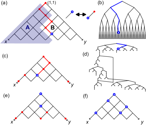
Figure 1: (a) The real space lattice and subregions $A$, $B$. Blue circled, red dotted and empty sites denote $|2\rangle_{\zeta_{\mathbf{R}}}$, $|1\rangle_{\zeta_{\mathbf{R}}}$ and $|0\rangle_{\zeta_{\mathbf{R}}}$, respectively. (a),(c),(e),(f) show Fock states (for small $L$) in four Krylov subspaces. (b) and (d) show the Fock space graphs of (a) and (c), respectively.

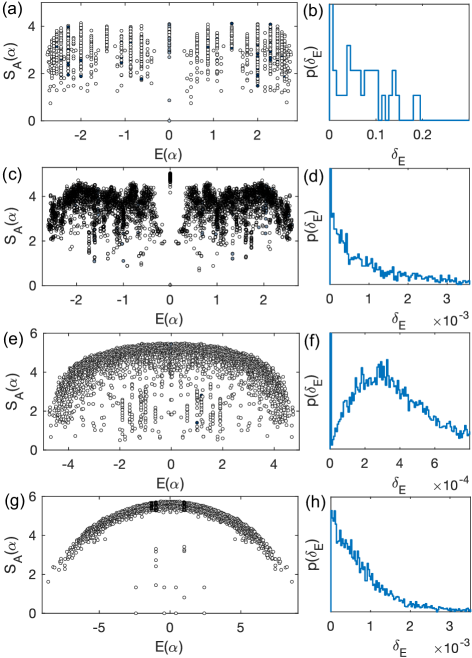
Figure 2: Numerical results at $W=0$ for $4$ Krylov subspaces illustrated in Fig. 1(a),(c),(e),(f) with layer number $L=13,7,7,5$, respectively. (a),(c),(e),(g) show their eigenstate entanglement entropy $S_{A}(\alpha)$ versus eigen-energy $E(\alpha)$, while (b),(d),(f),(h) show their LSS $p(\delta_{E})$.

At $W=0$, one has $V_{\mathbf{P}}=0$, and the model Eq. 4 in Cayley tree is integrable [60] and has energy levels $E_{l_{0},n}=-2\sqrt{2}\cos\left(\frac{n\pi}{L+2-l_{0}}\right)$ with level degeneracies $2^{l_{0}-2}+\frac{1}{2}\delta_{l_{0},1}$, where $1\leq l_{0}\leq L$ and $1\leq n\leq L+1-l_{0}$ (see SM [59] Sec. IV). Fig. 2(a) shows the ED numerical entanglement entropy $S_{A}(\alpha)$ (in half subregion $A$ of Fig. 1(a)) of all eigenstates $|\alpha\rangle$, where integer $\alpha$ sorts their energies $E(\alpha)$ from low to high. Fig. 2(b) shows the level spacing statistics (LSS) $p(\delta_{E})$ of $\delta_{E}(\alpha)=E(\alpha+1)-E(\alpha)$. Both results show irregular patterns because of the integrability at $W=0$.

To study localization at $W>0$, we first recall the standard Anderson localization model [61], which assumes random on-site potentials $V_{\mathbf{P}}$ uniformly distributed in an interval $[-\frac{\Lambda}{2},\frac{\Lambda}{2}]$. In the infinite $z=3$ Bethe lattice, analytical and numerical studies [45, 46, 47, 48, 49, 50] demonstrate the eigenstates become localized when $\Lambda>\Lambda_{*}\approx 16\sim 18$. In the Cayley tree (finite patch of Bethe lattice), localization is delicate due to finite ratio between boundary and bulk sites in the thermodynamic limit. By randomly connecting the boundary sites into coordination number $z=3$, an Anderson localization transition around $\Lambda_{*}$ can be observed [51] (see SM [59] Sec. V).

Our model Eq. 4 with $W>0$ defines a modified single-particle localization model with random potentials $V_{\mathbf{P}}=\sum_{\mathbf{R}\in\mathbf{P}}\epsilon_{\mathbf{R}}$, where $\epsilon_{\mathbf{R}}\in[-\frac{W}{2},\frac{W}{2}]$. Therefore, a particle traveling from site $\mathbf{P}$ to another site $\mathbf{P}^{\prime}$ distance $d_{\mathbf{P},\mathbf{P}^{\prime}}$ away in the Cayley tree graph feels a random potential difference $|V_{\mathbf{P}}-V_{\mathbf{P}^{\prime}}|\sim\sqrt{d_{\mathbf{P},\mathbf{P}^{\prime}}}W$. With the mean site distance $\langle d_{\mathbf{P},\mathbf{P}^{\prime}}\rangle\sim L$ in the Cayley tree, we estimate the effective on-site disorder strength as $\Lambda\sim|V_{\mathbf{P}}|_{\text{rms}}=\sqrt{\langle V_{\mathbf{P}}^{2}\rangle}\sim\sqrt{L}W$ (root mean square of $V_{\mathbf{P}}$), which we verified numerically (SM [59] Sec. VII). This suggests localization (MBL) in this Krylov subspace $\mathcal{K}_{1}$ to happen when $W>W_{*}\sim\frac{\Lambda_{*}}{\sqrt{L}}$, with $\Lambda_{*}\approx 16\sim 18$ defined earlier. Thus, $W_{*}\rightarrow 0$ in the thermodynamic limit $L\rightarrow\infty$.

Numerically, MBL would obey Poisson LSS $p(\delta_{E})\propto e^{-\delta_{E}/\lambda_{0}}$ [62], while the quantum chaotic thermalizing phase would obey Wigner-Dyson LSS (Gaussian orthogonal ensemble (GOE) for real Hamiltonian) $p(\delta_{E})\propto\delta_{E}e^{-(\delta_{E}/\lambda_{0})^{2}}$ [63, 64, 65], with $\lambda_{0}$ some constant. We calculate the LSS ratio $\langle r\rangle$ defined as the mean value of $r(\alpha)=\frac{\min\{\delta_{E}(\alpha),\delta_{E}(\alpha+1)\}}{\max\{\delta_{E}(\alpha),\delta_{E}(\alpha+1)\}}$ [26], which approaches $0.53$ for GOE and $0.39$ for Poisson [66]. Fig. 3(a) shows $\langle r\rangle$ (averaged over disorder samplings) with respect to $W$ in Krylov subspace $\mathcal{K}_{1}$ (Cayley tree with unconnected boundary sites) for different $L$ (up to $13$, given in legend), which stays below GOE for all $W$. Fig. 3(b) shows $\langle r\rangle$ after randomly connecting the Cayley tree boundary sites into coordination number $z=3$, which decreases from GOE to Poisson as $W$ increases. For $W>0$ ($W\gtrsim 5$) with unconnected (connected) boundaries, the $\langle r\rangle$ curves monotonically decrease towards Poisson with increasing $L$. This agrees with our expectation $W_{*}\sim\frac{\Lambda_{*}}{\sqrt{L}}$.

MBL in $\mathcal{K}_{1}$ manifests more clearly in the entanglement entropy $S_{A}(t)$ versus time $t$ with initial state being the root state $|\psi_{1}\rangle$. Fig. 3(c) (where $L=13$) shows for $W$ not too small, $S_{A}(t)\approx c_{A}\log t$ when $t<t_{*}$ and saturates clearly below the Page value (dashed line) when $t>t_{*}$, as expected for MBL. For fixed $W$, the coefficient $c_{A}$ is roughly independent of $L$, and the saturation time $t_{*}\sim e^{L/\xi}$ with some $\xi>0$, as shown in Fig. 3(d).

Figure 3: For one-boson Krylov subspace $\mathcal{K}_{1}$ which maps to Cayley tree, the LSS ratio $\langle r\rangle$ with (a) unconnected and (b) connected boundary; and the time-evolved entanglement entropy $S_{A}(t)$ (unconnected boundary) from the root state for (c) different $W$ at $L=13$, and (d) different $L$ at $W=4$ ($100$-sample average). (e)-(f) show $\langle r\rangle$ and $S_{A}(t)$ (for $L=7$) of the one-boson Krylov subspace $\mathcal{K}_{1,\mathcal{S}_{1}}$ (illustrated in Fig. 1(c)-(d)). The legends in (a),(b),(e) label the layer number $L$.

The fact that $\frac{\text{dim}\mathcal{K}_{1}}{\text{dim}\mathcal{H}_{\{Q_{m}=\delta_{m,1}\}}}\sim(2/L)^{L}$ indicates $\mathcal{K}_{1}$ is an exponentially small subspace of charge sector $\mathcal{H}_{\{Q_{m}=\delta_{m,1}\}}$. The other Krylov subspaces have smaller dimensions $2^{L+1-l_{K}}-1$ ($l_{K}>1$) (SM [59] Sec. III), and show similar MBL. Generically, most charge sectors fragment into exponentially many Krylov subspaces.

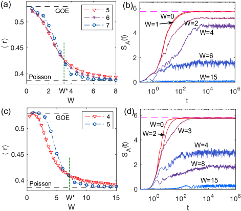
Figure 4: The LSS ratio $\langle r\rangle$, and time-evolved entanglement entropy $S_{A}(t)$ starting from the root state, for: (a)-(b) the two-boson Krylov subspace illustrated in Fig. 1(e), and (c)-(d) the five-boson Krylov subspace illustrated in Fig. 1(f). The legends in (a),(c) label the layer number $L$.

As an example in a different one-boson charge sector, we numerically construct the Krylov subspace $\mathcal{K}_{1,\mathcal{S}_{1}}$ generated by root state $|\psi_{1,\mathcal{S}_{1}}\rangle=|2\rangle_{1}\otimes\prod_{\zeta_{\mathbf{R}}\in\mathcal{S}_{1}}|1\rangle_{\zeta_{\mathbf{R}}}\otimes\prod_{\zeta_{\mathbf{R}}\notin\{1\}\cup\mathcal{S}_{1}}|0\rangle_{\zeta_{\mathbf{R}}}$, with a set of sites $\mathcal{S}_{1}=\{7+4k\ |\ k\geq 0\}$ in state $|1\rangle_{\zeta_{\mathbf{R}}}$ (Fig. 1(c)). The Hamiltonian in this Krylov subspace maps to a model similar to Eq. 4 in a Fock space graph $\mathcal{G}_{1,\mathcal{S}_{1}}$ as shown in Fig. 1(d), where the potential $V_{\mathbf{P}}=\sum_{\mathbf{R}}\epsilon_{\mathbf{R}}\langle\rho^{\uparrow}_{\mathbf{R}}\rangle_{\mathbf{P}}$ for graph site $\mathbf{P}$, with $\langle\rho^{\uparrow}_{\mathbf{R}}\rangle_{\mathbf{P}}=1$ or $0$ if site $\mathbf{R}$ has spin $\uparrow$ or $\downarrow$. The graph is more complicated than Cayley tree and has loops, although the average bulk coordination number remains $z\approx 3$. Numerically, we find $\mathcal{G}_{1,\mathcal{S}_{1}}$ has mean graph site distance $\langle d_{\mathbf{P},\mathbf{P}^{\prime}}\rangle\sim L^{3}$ (SM [59] Sec. VII), longer than the Cayley tree case. Since the total number of sites scales as $L^{2}$, we estimate the effective graph on-site disorder strength $\Lambda\sim|V_{\mathbf{P}}|_{\text{rms}}\sim\min(\sqrt{\langle d_{\mathbf{P},\mathbf{P}^{\prime}}\rangle}W,\sqrt{L^{2}}W)\sim LW$, which we verified numerically (SM [59] Sec. VII). Thus, we expect MBL to happen when $W>W_{*}\sim\frac{\Lambda_{*}}{L}$, again suggesting $W_{*}\rightarrow 0$ as $L\rightarrow\infty$.

Fig. 2(c)-(d) show the eigenstate entanglement entropy $S_{A}(\alpha)$ and LSS of Krylov subspace $\mathcal{K}_{1,\mathcal{S}_{1}}$ at $W=0$, which readily shows Poisson LSS except for a set of degenerate levels. Fig. 3(e) shows the LSS ratio $\langle r\rangle$ monotonically approaches Poisson at $W>0$ as $L$ increases. For all $W\geq 0$, the entanglement entropy evolved from the root state $|\psi_{1,\mathcal{S}_{1}}\rangle$ shows $S_{A}(t)\propto\log t$ when $t<t_{*}$ and saturates below the Page value (dashed line) when $t>t_{*}$, with $t_{*}\sim e^{L/\xi}$ (see Fig. 3(f) and SM [59]). This agrees with the expected MBL for $W>W_{*}\rightarrow 0$.

Multi-boson charge sectors. We now study Krylov subspaces $\mathcal{K}_{\mathcal{S}_{2},\mathcal{S}_{1}}$ generated by multi-boson root states of the form $|\psi_{\mathcal{S}_{2},\mathcal{S}_{1}}\rangle=\prod_{\zeta_{\mathbf{R}}\in\mathcal{S}_{2}}|2\rangle_{\zeta_{\mathbf{R}}}\otimes\prod_{\zeta_{\mathbf{R}}\in\mathcal{S}_{1}}|1\rangle_{\zeta_{\mathbf{R}}}\otimes\prod_{\zeta_{\mathbf{R}}\notin\mathcal{S}_{2}\cup\mathcal{S}_{1}}|0\rangle_{\zeta_{\mathbf{R}}}$, where $\mathcal{S}_{2}$ and $\mathcal{S}_{1}$ are the sets of sites in $|2\rangle_{\zeta_{\mathbf{R}}}$ and $|1\rangle_{\zeta_{\mathbf{R}}}$ states, respectively. We present two examples: (1) two-boson Krylov subspace generated by root state with $\mathcal{S}_{2}=\{1,5\}$ and $\mathcal{S}_{1}=\{7+2k\ |\ k\geq 0\}$ shown in Fig. 1(e); (2) five-boson Krylov subspace generated by root state with $\mathcal{S}_{2}=\{1,2,6,7,9\}$ and $\mathcal{S}_{1}$ empty as shown in Fig. 1(f).

At $W=0$, a multi-boson Krylov subspace can show either GOE or Poisson LSS, but generically retains certain solvable structures. Fig. 2(e)-(h) shows the eigenstate entanglement entropy $S_{A}(\alpha)$ and LSS in the above two-boson and five-boson Krylov subspaces, respectively, which indicates the former is quantum chaotic while the latter is potentially integrable. In both Krylov subspaces, a subset of eigenstates, a significant fraction of which have degeneracies, show significantly lower entanglement entropy than the mojarity eigenstates. In the chaotic two-boson case (Fig. 2(e)), this subset of eigenstates fulfill the definition of many-body quantum scar states.

At $W>0$, in both the two-boson and five-boson Krylov subspaces, the LSS ratio $\langle r\rangle$ varies from GOE to Poisson as $W$ increases (Fig. 4(a) and (c)), and the $\langle r\rangle$ curves for different $L$ (up the largest calculable $L$) intersect at certain $W=W_{*}$. The entanglement entropy time evolution from the root state shows $S_{A}(t)\propto t$ ($S_{A}(t)\propto\log t$) at early $t$ and saturation at (below) the Page value at late $t$ for small (large) $W$ (Fig. 4(b) and (d)), implying a transition from thermalization ($W<W_{*}$) to MBL ($W>W_{*}$).

A $N_{b}$-boson Krylov subspace generically maps to a complicated Fock space graph $\mathcal{G}_{\mathcal{S}_{2},\mathcal{S}_{1}}$ with numerous loops and with average coordination number $z\approx 2N_{b}+1$ (as each boson can move in two directions). Numerically, the mean graph distance scales as $\langle d_{\mathbf{P},\mathbf{P}^{\prime}}\rangle\sim L^{\eta}$ in $L$, with $\eta\approx 3$ in both (two-boson and five-boson) Krylov subspaces here. This upper bounds the effective graph on-site disorder strength $\Lambda\sim|V_{\mathbf{P}}|_{\text{rms}}\lesssim\min(\sqrt{\langle d_{\mathbf{P},\mathbf{P}^{\prime}}\rangle}W,\sqrt{L^{2}}W)$. Indeed, we numerically find $|V_{\mathbf{P}}|_{\text{rms}}\sim L^{\gamma}W$, with $\frac{1}{2}\leq\gamma\leq\min(\frac{\eta}{2},1)$. For the above two-boson and five-boson Krylov subspaces, $\gamma\approx 1$ and $\frac{1}{2}$, respectively (see SM [59] Sec. VII). Thus, we expect MBL to happen when $W>W_{*}\sim\frac{\Lambda_{*}(z)}{L^{\gamma}}$, where $\Lambda_{*}(z)$ is the standard Anderson transition point in graphs with coordination number $z$, which scales as $\Lambda_{*}(z)\propto z\log z\sim N_{b}\log N_{b}$ when $N_{b}$ is large [45, 47]. Particularly, $W_{*}$ would be finite or zero if $N_{b}\lesssim L^{\gamma}/\log L$ when taking the thermodynamic limit $L\rightarrow\infty$.

Discussion. We have shown that our 2d quantum breakdown model strongly fragments into Krylov subspace exhibiting MBL beyond certain disorder strength $W_{*}$, with $W_{*}$ finite in the thermodynamic limit if $N_{b}\lesssim L^{\gamma}/\log L$ ($\frac{1}{2}\leq\gamma\leq 1$). Heuristically, this MBL emerges from particles interacting with a swampland of spin configurations which would be non-dynamical without the particles. This may allow generalization into a class of MBL models, and provide understandings of generic preconditions for achieving higher dimensional MBL. Moreover, it will be intriguing to explore potential realizations of such models in experiments such as Rydberg atoms, and the effects from perturbations respecting or breaking the subsystem symmetries.

Appendix A Supplementary Material

Appendix B I. Hamiltonian in the truncated on-site basis

By defining on-site states $|0\rangle_{\zeta_{\mathbf{R}}}$ (the unexcited state with spin $\downarrow$ and zero boson), $|1\rangle_{\zeta_{\mathbf{R}}}=\sigma_{+,\mathbf{R}}|0\rangle_{\zeta_{\mathbf{R}}}$, $|2\rangle_{\zeta_{\mathbf{R}}}=b^{\dagger}_{\mathbf{R}}\sigma_{+,\mathbf{R}}|0\rangle_{\zeta_{\mathbf{R}}}$ and $|3\rangle_{\zeta_{\mathbf{R}}}=b^{\dagger}_{\mathbf{R}}|0\rangle_{\zeta_{\mathbf{R}}}$, we note that the Hamiltonian cannot access on-site state $|3\rangle_{\zeta_{\mathbf{R}}}$ unless there are such sites initially. In this paper, we exclude such on-site states to simplify our model, namely, on each site $\mathbf{R}$, we only keep three basis states: $\left(|2\rangle_{\zeta_{\mathbf{R}}},|1\rangle_{\zeta_{\mathbf{R}}},|0\rangle_{\zeta_{\mathbf{R}}}\right)$. The reduced Hamiltonian of main text Eq. (1) then becomes

$$\begin{split}&H=\sum_{\mathbf{R}}\Big{[}\epsilon_{\mathbf{R}}\rho^{\uparrow}_{\mathbf{R}}-\sum_{\nu=x,y}\left(A^{\dagger}_{\mathbf{R}+\mathbf{e}_{\nu}}B_{\mathbf{R}}+h.c.\right)\Big{]}\ ,\end{split}$$ (S1)

where the operators on site $\mathbf{R}$ are defined in the basis $\left(|2\rangle_{\zeta_{\mathbf{R}}},|1\rangle_{\zeta_{\mathbf{R}}},|0\rangle_{\zeta_{\mathbf{R}}}\right)$ as

$$\begin{split}&\rho^{\uparrow}_{\mathbf{R}}=\left(\begin{array}[]{ccc}1&0&0\\ 0&1&0\\ 0&0&0\\ \end{array}\right),A_{\mathbf{R}}^{\dagger}=\left(\begin{array}[]{ccc}0&0&1\\ 0&0&0\\ 0&0&0\\ \end{array}\right),B_{\mathbf{R}}=\left(\begin{array}[]{ccc}0&0&0\\ 1&0&0\\ 0&0&0\\ \end{array}\right)\ .\end{split}$$ (S2)

Appendix C II. Derivation of the conserved subsystem symmetry charges

Here we derive the subsystem symmetry charges in main text Eq. (3). The constrained model, in the form of Eq. S1 only contains three on-site states $(|2\rangle_{\zeta_{\mathbf{R}}},|1\rangle_{\zeta_{\mathbf{R}}},|0\rangle_{\zeta_{\mathbf{R}}})$. We assign the three states $\{|2\rangle_{\zeta_{\mathbf{R}}},|1\rangle_{\zeta_{\mathbf{R}}},|0\rangle_{\zeta_{\mathbf{R}}}\}$ in a site $\mathbf{R}$ in layer $l$ three U(1) charges $\{q^{l},q^{l}(1-q),0\}$, respectively, where $q$ is an arbitrary number. Note that the interaction term $\sigma_{+,\mathbf{R}+\mathbf{e}_{\nu}}b^{\dagger}_{\mathbf{R}+\mathbf{e}_{\nu}}b_{\mathbf{R}}\rho^{\uparrow}_{\mathbf{R}}+h.c.$ in main text Eq. (1), or equivalently $A^{\dagger}_{\mathbf{R}+\mathbf{e}_{\nu}}B_{\mathbf{R}}+h.c.$ in Eq. S1, changes an on-site state $|2\rangle_{\mathbf{R}}$ in layer $l$ with charge $q^{l}$ into a state $|1\rangle_{\zeta_{\mathbf{R}}}$ in layer $l$ with charge $q^{l}(1-q)$ and a state $|2\rangle_{{\zeta_{\mathbf{R}^{\prime}}}}$ in layer $l+1$ with charge $q^{l+1}$, after which the total U(1) charge is unchanged. Therefore, the total charge of the lattice

$$C(q)=\sum_{l=1}^{L}\left[q^{l}N_{2,l}+q^{l}(1-q)N_{1,l}\right]=\sum_{m=1}^{L+1}q^{m}Q_{m}$$ (S3)

is conserved, where we have defined $N_{j,l}=\sum_{\mathbf{R}\in l}|j\rangle\langle j|_{\zeta_{\mathbf{R}}}$ as the number of sites in layer $l$ which are in on-site state $|j\rangle_{\zeta_{\mathbf{R}}}$ ($j=1,2$). In the rewritten form power series form, the coefficients $Q_{m}$ ($1\leq m\leq L+1$) in Eq. S3 can be derived as

$$\begin{split}&Q_{1}=N_{2,1}+N_{1,1}\ ,\\ &Q_{m}=N_{2,m}+N_{1,m}-N_{1,m-1},\qquad(2\leq m\leq L)\\ &Q_{L+1}=-N_{1,L}\ .\end{split}$$ (S4)

which can be summarized into the form of main text Eq. (3). Since $q$ is an arbitrary number, we conclude that each $Q_{m}$ has to be conserved to make all $C(q)$ conserved. Therefore, each $Q_{m}$ is a subsystem symmetry conserved charge involving only at most two layers $m$ and $m+1$. In particular, the boson number $N_{b}=\sum_{\mathbf{R}}b^{\dagger}_{\mathbf{R}}b_{\mathbf{R}}=\sum_{l=1}^{L}N_{2,l}=\sum_{m=1}^{L+1}Q_{m}$ is a global conserved charge.

Appendix D III. Hilbert space dimension of charge sector $\{Q_{m}=\delta_{m,1}\}$ and its Krylov subspaces

Here we derive the Hilbert space dimension of the one-boson charge sector with subsymmetry charges $Q_{m}=\delta_{m,1}$, as illustrated in main text Fig. 1(a). We then derive the dimensions of Krylov subspaces of the charge sector.

With $Q_{m}=\delta_{m,1}$, we have $N_{1,L}=0$, $N_{2,m}=N_{1,m-1}-N_{1,m}$, and $N_{2,1}=1-N_{1,1}$. Consider configurations with $N_{2,m}=\delta_{m,l}$ $(1\leq l\leq L)$, for which we would have $N_{1,m}=1$ if $m<l$, and $N_{1,m}=0$ if $m\geq l$. Therefore, in each layer $m\leq l$, there is one site not in state $|0\rangle_{\zeta_{\mathbf{R}}}$. Since there are $m$ sites in layer $m$, the position of this site has $m$ choices, and thus in total there are $\prod_{m=1}^{l}m=l!$ configurations with $N_{2,m}=\delta_{m,l}$. Thus, the total Hilbert space dimension of this charge sector is

$$\text{dim}\mathcal{H}_{\{Q_{m}=\delta_{m,1}\}}=\sum_{l=1}^{L}l!>L!\sim L^{L}\ .$$ (S5)

We now turn to Krylov subspaces in this charge sector $\mathcal{H}_{\{Q_{m}=\delta_{m,1}\}}$. In the main text, we considered the Krylov subspace $\mathcal{K}_{1}$ from root state $|\psi_{1}\rangle=|2\rangle_{1}\otimes\prod_{\zeta_{\mathbf{R}}\neq 1}|0\rangle_{\zeta_{\mathbf{R}}}$, in which the site $(1,1)$ in layer $1$ is in state $|2\rangle_{1}$ with a boson. As illustrated in main text Fig. 1(a), all the Fock states connected with $|\psi_{1}\rangle$ can be mapped into paths extended from site $(1,1)$ to the other sites $\mathbf{R}$, and all the paths map to the sites of a Cayley tree graph of $L$ layers. Since the number of paths reaching layer $l$ is $2^{l-1}$, the total Hilbert space dimension of Krylov subspace $\mathcal{K}_{1}$ is

$$\text{dim}\mathcal{K}_{1}=\sum_{l=1}^{L}2^{l-1}=2^{L}-1\ .$$ (S6)

Generically, a root state in this charge sector $\mathcal{H}_{\{Q_{m}=\delta_{m,1}\}}$ can be chosen as a Fock state $|\psi_{l_{K}}\rangle$ with one site with a boson (namely, state $|2\rangle_{\zeta_{\mathbf{R}}}$) in layer $l_{K}$, one site in state $|1\rangle_{\zeta_{\mathbf{R}}}$ in each layer $l<l_{K}$, and all the other sites in state $|0\rangle_{\zeta_{\mathbf{R}}}$, with a particular requirement that the site of state $|2\rangle_{\zeta_{\mathbf{R}}}$ in layer $l_{K}$ is not the nearest neighbor of the site of state $|1\rangle_{\zeta_{\mathbf{R}}}$ in layer $l_{K}-1$. Each such root state $|\psi_{l_{K}}\rangle$ can generate a Krylov subspace $\mathcal{K}_{l_{K}}$ of a Cayley tree of $L-l_{K}+1$ layers, in which each Fock state maps to a path from the root state boson site in layer $l_{K}$ to larger layers $l\geq l_{K}$, similar to $\mathcal{K}_{1}$. Thus, it has a Hilbert space dimension

$$\text{dim}\mathcal{K}_{l_{K}}=\sum_{l=l_{K}}^{L}2^{l-l_{K}}=2^{L+1-l_{K}}-1\ .$$ (S7)

The number of Krylov subspaces with this dimension is given by the number of distinct root states $|\psi_{l_{K}}\rangle$ satisfying the above requirement. For $l_{K}>1$, this gives the number of such Krylov subspaces:

$$D_{K}(l_{K})=(l_{K}-2)![(l_{K}-3)(l_{K}-2)+2(l_{K}-2)]=l_{K}!-2(l_{K}-1)!\ ,\qquad(l_{K}>1)$$ (S8)

and for $l_{K}=1$, one has $D_{K}(1)=1$. Therefore, the number of Krylov subspaces in this charge sector is exponentially large.

Generically, one can show that most the charge sectors have exponentially large number of Krylov subspaces.

Appendix E IV. Exact solution at $W=0$ in Krylov subspace $\mathcal{K}_{1}$ (tight binding model in the Cayley tree)

At disorder $W=0$, the model in the Krylov subspace $\mathcal{K}_{1}$, or equivalently the tight-binding model in a Cayley tree (main text Eq. (5)), is exactly solvable [60]. Here we derive the eigenstates and eigen-energies.

Since each Fock state corresponds to a path $\mathbf{P}$ of length up to $L-1$ in the real space, we can relabel each Fock state $|\mathbf{P}\rangle$ with a binary string of length $L$ of the form

$$|n_{1}n_{2}\cdots n_{L}\rangle\ ,$$ (S9)

where $n_{j}=0$ or $1$. For a path of $l-1$ steps which reaches layer $l$, the rightmost nonzero digit will be $n_{l}=1$, while for all $l^{\prime}>l$, one has $n_{l^{\prime}}=0$; for $l^{\prime}<l$, we define $n_{l^{\prime}}=1$ ($n_{l^{\prime}}=0$) if the $l^{\prime}$-th step of the path moves in the $\mathbf{e}_{x}$ ($\mathbf{e}_{y}$) direction. This gives a unique labeling of all the $2^{L}-1$ paths (Fock states) in $\mathcal{K}_{1}$.

The key to solve for the eigenstates exactly is to observe that, at $W=0$, the Krylov subspace $\mathcal{K}_{1}$ further fragments into smaller Krylov subspaces. These smaller Krylov subspaces are generated by root states orthogonal to each other. Such a generic root state is a state of superposition of two paths reaching layer $l_{0}$ (path of $l_{0}-1$ steps):

$$\begin{split}&|\psi^{1}\rangle=|100\cdots 0\rangle\ ,\\ &|\psi^{l_{0}}_{n_{1}n_{2}\cdots n_{l_{0}-2}}\rangle=\frac{1}{\sqrt{2}}\sum_{n_{l_{0}-1}=0}^{1}(-1)^{n_{l_{0}-1}}|n_{1}n_{2}\cdots n_{l_{0}-2}n_{l_{0}-1}100\cdots 0\rangle\ ,\qquad(l_{0}\geq 2)\end{split}$$ (S10)

where $n_{1}n_{2}\cdots n_{l_{0}-2}$ is a binary string of $0$ or $1$. For $l_{0}\geq 2$, since the two Fock state components have opposite signs, one can show this root state cannot hop to any states of paths reaching layer $l<l_{0}$, thus $l_{0}$ is the smallest layer the state can hop to. But the root state can hop to larger layers $l>l_{0}$. The state with paths reaching layer $l>l_{0}$ which the above root states can hop to generically takes the form:

$$\begin{split}&|\psi^{1,l}\rangle=\frac{1}{2^{(l-1)/2}}\sum_{n_{l_{0}-1},\cdots,n_{l-1}=0}^{1}|n_{1}n_{2}\cdots n_{l-1}100\cdots 0\rangle\ ,\qquad(l\geq 1)\\ &|\psi^{l_{0},l}_{n_{1}n_{2}\cdots n_{l_{0}-2}}\rangle=\frac{1}{2^{(l+1-l_{0})/2}}\sum_{n_{l_{0}-1},\cdots,n_{l-1}=0}^{1}(-1)^{n_{l_{0}-1}}|n_{1}n_{2}\cdots n_{l_{0}-2}n_{l_{0}-1}\cdots n_{l-1}100\cdots 0\rangle\ ,\qquad(l\geq l_{0}\geq 2).\end{split}$$ (S11)

It is straightforward to show that for a fixed $l_{0}$, the $L-l_{0}+1$ states $|\psi^{l_{0},l}_{n_{1}n_{2}\cdots n_{l_{0}-2}}\rangle$ (with $l_{0}\leq l\leq L$) form a closed Krylov subspace, in which the zero disorder Hamiltonian $H$ takes the form of a one-dimensional open boundary tight-binding model with hopping amplitude $-\sqrt{2}$:

$$H|\psi^{l_{0},l}_{n_{1}n_{2}\cdots n_{l_{0}-2}}\rangle=-\sqrt{2}\Big{(}\Theta_{L-l}|\psi^{l_{0},l+1}_{n_{1}n_{2}\cdots n_{l_{0}-2}}\rangle+\Theta_{l-l_{0}}|\psi^{l_{0},l-1}_{n_{1}n_{2}\cdots n_{l_{0}-2}}\rangle\Big{)}\ ,$$ (S12)

where we define $\Theta_{n}=1$ if $n>0$ and $\Theta_{n}=0$ if $n\leq 0$. Therefore, the eigen-energies of this subspace is given by

$$E_{l_{0},n}=-2\sqrt{2}\cos\left(\frac{n\pi}{L+2-l_{0}}\right)\ .$$ (S13)

The level degeneracy is given by the number of different root states in layer $l_{0}$ in Eq. S10, which is the number of choices of the binary string $n_{1}n_{2}\cdots n_{l_{0}-2}$. This gives a level degeneracy $2^{l_{0}-2}+\frac{1}{2}\delta_{l_{0},1}$ (note the fact that the degeneracy is $1$ when $l_{0}=1$.)

Appendix F V. Comparing the Modified and the Standard Anderson Localization problem on Cayley tree

In the main text Fig. 3(a)-(b), we have shown the full spectrum LSS ratio $\langle r\rangle$ of our model in Krylov subspace $\mathcal{K}_{1}$, which maps to a modified Anderson localization problem (main text Eq. (5)) in the Cayley tree in Fock space. As $L$ increases (calculated up to $13$), the $\langle r\rangle$ curves with respect to disorder strength $W$ of different $L$ for unconnected boundary (which is our model) decrease towards Poisson, while those for randomly connected boundary (into coordination number $z=3$, which is modified on top of our model) decrease towards Poisson for $W\gtrsim 5$ and remain almost unchanged for $W\lesssim 5$. Fig. S1(g)-(h) show the LSS probability function $p(\delta_{E})$ (averaged over many samplings) for unconnected (blue solid line) and connected (red dashed line) boundary, at $W=1$ and $W=20$, respectively. For unconnected boundary, the LSS deviates from GOE Wigner-Dyson function significantly at small $W$.

Figure S1: (a)-(b) The full spectrum $\langle r\rangle$ and (c)-(d) the central spectrum $\langle r\rangle$ of the standard Anderson localization model in the Cayley tree, with unconnected or connected boundary. (e)-(f) The central spectrum $\langle r\rangle$ of our model in Krylov subspace $\mathcal{K}_{1}$ with unconnected or connected boundary. (g)-(h) The full spectrum LSS probability distribution of our model with unconnected or connected boundary (averaged over many disorder samplings).

In comparison, for the standard Anderson localization problem in the Cayley tree, which has on-site potential in main text Eq. (5) uniformly distributed in

$$V_{\mathbf{P}}\in[-\Lambda/2,\Lambda/2]\ ,$$ (S14)

the LSS ratio $\langle r\rangle$ (averaged over many samplings) of the full spectrum with unconnected boundary is shown in Fig. S1(a), and that with boundary randomly connected into coordination number $z=3$ is shown in Fig. S1(b). As $L$ increases (calculated up to $13$), the unconnected boundary $\langle r\rangle$ curves with respect to $\Lambda$ also monotonically decreases, while the connected boundary $\langle r\rangle$ curves for different $L$ intersects around $\Lambda_{*}\approx 13$, signaling an Anderson transition (close to the Bethe lattice value $\Lambda_{*}\approx 16\sim 18$). This is similar to the observation in Ref. [51].

The center of the energy spectrum is generically more difficult to localize. Therefore, we also calculate the central spectrum LSS ratio $\langle r\rangle$ of the energy levels within an energy window of width $0.1(E_{\text{max}}-E_{\text{min}})$ at the center of the spectrum, where $E_{\text{max}}$ and $E_{\text{min}}$ are the maximal and minimal energy of the spectrum, respectively. Fig. S1(c)-(d) shows the central spectrum $\langle r\rangle$ of the standard Anderson problem with unconnected and connected boundary, respectively. The connected boundary figure shows a transition point slightly higher, around $\Lambda_{*}\approx 14$. In comparison, Fig. S1(e)-(f) show the central spectrum LSS ratio of our model in Krylov subspace $\mathcal{K}_{1}$ (modified Anderson model in Cayley tree, main text Eq. (5)) with unconnected and connected boundary, respectively. The connected boundary result Fig. S1(f) shows a transition around $W_{*}\approx 6\sim 7$. As argued in the main text, we expect $W_{*}\sim\frac{\Lambda_{*}}{\sqrt{L}}$, which is serves as a good estimation.

Appendix G VI. Example of loops in the Fock space graph

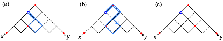
Figure S2: Illustration of a loop in the 1-boson Krylov subspace $\mathcal{K}_{1,\mathcal{S}_{1}}$. Starting from the same Fock state, (a) and (b) show two different paths which end up at the same Fock state in (c).

For the 1-boson Krylov subspace $\mathcal{K}_{1,\mathcal{S}_{1}}$ we studied, illustrated in main text Fig. 1(c), which is generated by root state $|\psi_{1,\mathcal{S}_{1}}\rangle=|2\rangle_{1}\otimes\prod_{\zeta_{\mathbf{R}}\in\mathcal{S}_{1}}|1\rangle_{\zeta_{\mathbf{R}}}\otimes\prod_{\zeta_{\mathbf{R}}\notin\{1\}\cup\mathcal{S}_{1}}|0\rangle_{\zeta_{\mathbf{R}}}$, with a set of sites $\mathcal{S}_{1}=\{7+4k\ |\ k\geq 0\}$ in state $|1\rangle_{\zeta_{\mathbf{R}}}$, its Fock space graph contain loops as shown in main text Fig. 1(d). Fig. S2 shows how a loop in this Fock space graph looks like in the real space: (a) and (b) show two different paths of the boson, which end up at the same Fock state in (c).

Appendix H VII. System size scaling of Fock space graph distances and graph on-site potentials

For the Fock space graphs of the four Krylov subspaces we considered in the main text (illustrated in main text Fig. 1):

$$\begin{split}&\text{(1) one-boson Krylov (Cayley tree) }\mathcal{K}_{1}\ ,\\ &\text{(2) one boson Krylov}\qquad\qquad\qquad\mathcal{K}_{1,\mathcal{S}_{1}}\ ,\qquad\mathcal{S}_{1}=\{7+4k\ |\ k\geq 0\}\\ &\text{(3) two-boson Krylov}\qquad\qquad\qquad\mathcal{K}_{\mathcal{S}_{2},\mathcal{S}_{1}}\ ,\qquad\mathcal{S}_{2}=\{1,5\}\ ,\quad\mathcal{S}_{1}=\{7+2k\ |\ k\geq 0\}\\ &\text{(4) five-boson Krylov}\qquad\qquad\qquad\mathcal{K}_{\mathcal{S}_{2},\mathcal{S}_{1}}\ ,\qquad\mathcal{S}_{2}=\{1,2,6,7,9\}\ ,\quad\mathcal{S}_{1}=\emptyset\ ,\end{split}$$ (S15)

we numerically calculate the mean graph distance $\langle d\rangle=\langle d_{\mathbf{P},\mathbf{P}^{\prime}}\rangle$ between two arbitrary graph sites $\mathbf{P}$ and $\mathbf{P}^{\prime}$ and its standard deviation $\delta d$. The resulting $\langle d\rangle\pm\delta d$ for different system sizes $L$ are shown in Fig. S3(a),(c),(e),(g), for the four Krylov subspaces in Eq. S15, respectively. In particular, we find $\langle d\rangle\propto L$ in the one-boson Krylov subspace $\mathcal{K}_{1}$ (Cayley tree) (Fig. S3(a)), and $\langle d\rangle\propto L^{3}$ in the other three Krylov subspaces (Fig. S3(c),(e),(g)).

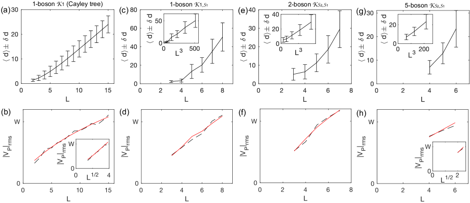
Figure S3: For the four Krylov subspaces we considered in the main text (listed in Eq. S15, see also Fig. 1), (a),(c),(e),(g) show the numerical mean Fock-space graph distance $\langle d\rangle$ between two graph sites, with standard deviation $\delta d$, with respect to system size (number of layers) $L$. (b),(d),(f),(h) show the corresponding (the same column) root mean square value $|V_{\mathbf{P}}|_{\text{rms}}=\sqrt{\langle V_{\mathbf{P}}^{2}\rangle}$ of graph on-site potential $V_{\mathbf{P}}$ with respect to $L$.

We further numerically calculate the root mean square value $|V_{\mathbf{P}}|_{\text{rms}}=\sqrt{\langle V_{\mathbf{P}}^{2}\rangle}$ of the graph on-site potential $V_{\mathbf{P}}=\sum_{\mathbf{R}}\epsilon_{\mathbf{R}}\langle\rho^{\uparrow}_{\mathbf{R}}\rangle_{\mathbf{P}}$, which are shown in Fig. S3(b),(d),(f),(h) for the four Krylov subspaces in Eq. S15, respectively. The black dashed lines show the values averaged from a large number of disorder samplings, while the red solid line is calculated from the simple rule of square summation:

$$\langle V_{\mathbf{P}}^{2}\rangle=\sum_{\mathbf{R}}\langle\rho^{\uparrow}_{\mathbf{R}}\rangle_{\mathbf{P}}\langle\epsilon_{\mathbf{R}}^{2}\rangle=\frac{W^{2}}{12}\sum_{\mathbf{R}}\langle\rho^{\uparrow}_{\mathbf{R}}\rangle_{\mathbf{P}}\ ,$$ (S16)

where $\langle\rho^{\uparrow}_{\mathbf{R}}\rangle_{\mathbf{P}}=0$ or $1$ if the site has spin $\downarrow$ or $\uparrow$, and $\langle\epsilon_{\mathbf{R}}^{2}\rangle=W^{2}/12$ is the mean square of $\epsilon_{\mathbf{R}}$. The two results (black dashed lines and red solid lines) agree well. The results show $|V_{\mathbf{P}}|_{\text{rms}}\propto L^{\gamma}W$, with the exponent $\gamma\approx\frac{1}{2},1,1,\frac{1}{2}$ for the four Krylov subspaces in Eq. S15, respectively.

Appendix I VIII. System size scaling of entanglement entropy time evolution

Fig. S4(a),(b),(c) show the time evolution (averaged over many disorder samplings) of entanglement entropy $S_{A}(t)$ with the initial state being the root state, for fixed $W$ and different system sizes $L$, for the Krylov subspaces (2),(3),(4) in Eq. S15, respectively. In all the cases, $S_{A}(t)\propto\log t$ at early time $t$ and saturates at late time $t$. The time $t_{*}$ for achieving saturation scales at least as $t_{*}\sim e^{L/\xi}$ with some $\xi>0$.

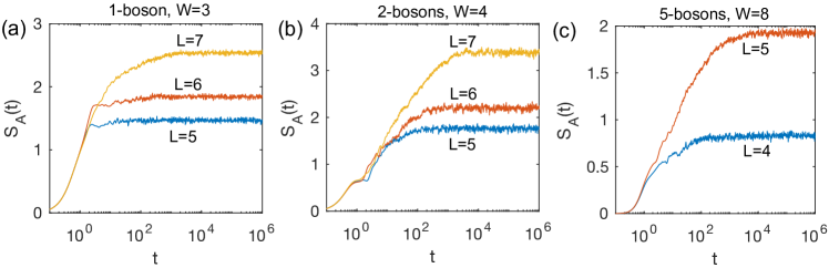
Figure S4: time evolution (averaged over many disorder samplings) of entanglement entropy $S_{A}(t)$ from the root state, for fixed $W$ and different system sizes $L$. (a),(b) and (c) are for the Krylov subspaces (2) (one-boson),(3) (two-boson),(4)(five-boson) in Eq. S15, respectively.