Learning DFAs from Confidence Oracles

1 Introduction

In this report, we discuss the problem of learning a deterministic finite automaton (DFA) from a confidence oracle. That is, we are given access to an oracle $Q$ with incomplete knowledge of some target language $L$ over an alphabet $\Sigma$; the oracle maps a string $x\in\Sigma^{*}$ to a score in the interval $[-1,1]$ indicating its confidence that the string is in the language. The interpretation is that the sign of the score signifies whether $x\in L$, while the magnitude $|Q(x)|$ represents the oracle’s confidence. Our goal is to learn a DFA representation of the oracle that preserves the information that it is confident in. That is, the learned DFA should closely match the oracle wherever it is highly confident, but it need not do this when the oracle is less sure of itself.

1.1 Motivation

We will begin by providing a couple examples of confidence oracles that may be encountered in practice. For one, consider a recurrent neural network (RNN) that maps finite strings in $\Sigma^{*}$ to scores in the interval $[-1,1]$ (e.g. the last layer is a $\tanh$ nonlinearity). The RNN outputs can be interpreted in exactly the same way as described for confidence oracles; i.e., the sign of the score is the classification of whether the string is in the language, while the magnitude is the RNN’s confidence. Moreover, we can include prior knowledge about the RNN in this confidence. For example, it may be reasonable to believe that the RNN’s accuracy decreases with the length of the input string (either because the RNN was not trained on long strings, or due to the problem of vanishing gradients [1]). If this is the case, we may simply multiply the RNN’s outputs with a factor that penalizes long strings.

For another example, consider a random process (e.g. a simulation with random initializations and/or dynamics) that returns a trace $x$ sampled from some distribution $X$ and a binary classification $y\sim Y$ for the trace. We can collect these outputs into a dataset of independent and identically distributed samples $\{(x_{i},y_{i})\}_{i\in[N]}$ and calculate the empirical prior probability $\Pr[Y=1\mid X]$. This probability, when normalized to the interval $[-1,1]$, can again be treated as a confidence oracle.

For each of the above examples, the original representation of the confidence oracle is cumbersome in some way. For instance, modern RNNs may contain millions of parameters, and it is often difficult for humans to explain or understand their reasoning. Similar problems arise when considering e.g. a simulation with random outcomes. Therefore, it is desirable to, using only black-box access, learn a more compact representation for these oracles. DFAs are a natural choice—they are relatively space/time efficient, and when small enough can be easily understood by simply examining their transition graphs. Moreover, model-checking of desired properties is better understood for automata than for any of the other representations mentioned.

1.2 Notation

A DFA $A$ is defined as a tuple

$$A\vcentcolon=(S,\Sigma,\delta,s_{0},F)$$

where $S$ is the set of states, $\Sigma$ is the alphabet, $\delta:S\times\Sigma\longrightarrow S$ is the transition function, $s_{0}\in S$ is the initial state, and $F\subseteq S$ are the accepting states. For strings of length $k$, we recursively extend the transition function

$$\delta^{*}(s,x)=\delta(\delta^{*}(s,x_{1}\ldots x_{k-1}),x_{k}).$$

For this report, we will conflate a DFA $A$ with its associated language

$$L_{A}\vcentcolon=\{x\in\Sigma^{*}\mid\delta^{*}(s_{0},x)\in F\}.$$

We will also conflate any language $L\subseteq\Sigma^{*}$ with the indicator function $\chi_{L}:\Sigma^{*}\longrightarrow\{-1,1\}$ defined as

$$\chi_{L}(x)\vcentcolon=\begin{cases}1&x\in L\\ -1&x\not\in L.\end{cases}$$

1.3 Problem Statement

Formally, we are given a finite alphabet $\Sigma$, along with an oracle $Q:\Sigma^{*}\longrightarrow[-1,1]$. For any other language $A:\Sigma^{*}\longrightarrow\{-1,1\}$, we define the distance

$$d(Q,A)\vcentcolon=\sum_{x\in\Sigma^{*}}|Q(x)|\cdot\mathbf{1}\{\operatorname{sgn}(Q(x))\neq A(x)\}.$$

That is, the distance $d(Q,A)$ is the sum of $Q$’s confidences where the sign of $Q(x)$ differs from $A(x)$. This definition captures the fact that we are interested in being close to $Q$ only whenever it is confident.

Let $\mathcal{R}_{\Sigma}$ be the set of regular languages over $\Sigma$. For a given $\eta>0$, the problem we wish to solve is

$$\min_{A\in\mathcal{R}_{\Sigma}} |A|$$ (1)

s.t. $$d(Q,A)\leq\eta,$$

where $|\cdot|:\mathcal{R}_{\Sigma}\longrightarrow\mathbb{N}$ maps a regular language to the number of states in its DFA representation. For practical purposes, it suffices to find a bicriteria approximation algorithm for this optimization problem. That is, letting $A^{*}$ be the optimal solution to (1), we hope for an algorithm that, given $Q$ and $\eta$, returns some automaton $\hat{A}$ such that $|\hat{A}|\in\poly(|A^{*}|)$ and $d(Q,\hat{A})\leq c\eta$ for some $\eta$.

For this report, we will also make some assumptions about the oracle $Q$:

• The sum of $Q$’s confidences converges:

  $$\sum_{x\in\Sigma^{*}}|Q|<\infty.$$

  This is really the regime we are interested in, for if the sum does not converge, any $A$ such $d(Q,A)$ is finite must agree with $Q$ at infinite locations. For a concrete example, consider a $Q$ that assigns equal weight to any two strings of equal length (that is, the confidence is determined solely by the length). Then, if $\sum_{x\in\Sigma^{*}}|Q|$ diverges, for any $A$ such that $d(Q,A)<\infty$, we must necessarily have

  $$\sum_{x\in\Sigma^{k}}\mathbf{1}\{\operatorname{sgn}(Q(x))\neq A(x)\}\longrightarrow 0$$

  as $k$ approaches infinity. That is, the discrepancy between $A$ and $Q$ must tend to zero as string length increases. This kind of behavior is not very relevant to our practical motivations.

  As another consideration, it is likely difficult for an algorithm to learn a hypothesis $A$ that agrees with $Q$ on infinite strings using only finite queries, especially since no equivalence queries are available (as opposed to the setting of Angluin’s $L^{*}$ algorithm).

  Assuming that the confidences converge, we can of course normalize such that without loss of generality

  $$\sum_{x\in\Sigma^{*}}|Q|=1.$$

  That is, the confidences of $Q$ form a probability distribution on $\Sigma^{*}$. Then, we can interpret the distance as

  $$d(Q,A)=\Pr[\operatorname{sgn}(Q(x))\neq A(x)]$$

  when $x$ is sampled from this distribution.

• We assume the distribution defined by $|Q|$ is given in some closed-form expression. In particular, it is easy to sample $x\sim|Q|$ and to evaluate the cumulative distribution function $\Pr[|x|\leq k]$. Alternatively, we can assume that $Q$ is enveloped by such a closed-form expression, i.e.

  $$\forall x\in\Sigma^{*}:Q(x)\leq P(x)$$

  and $P$ has the properties we desire. This is a reasonable assumption; if we had only query access to $|Q|$, the oracle could simply hide all of its weight on a single string which we could not find without a search through exponentially many candidates.

1.4 Interpretation as a metric space

Given an oracle $Q$, we can split the information it provides into two parts: a measure $\pi_{Q}:2^{\Sigma^{*}}\longrightarrow\mathbb{R}_{+}$ defined as

$$\pi_{Q}(S)\vcentcolon=\sum_{x\in S}|Q(x)|$$

and a language $L_{Q}$ defined as

$$L_{Q}=\{x\in\Sigma^{*}\mid Q(x)\geq 0\}.$$

Given our assumption that the confidences converge, we can normalize such that $\pi_{Q}(\Sigma^{*})=1$; i.e., $\pi_{Q}$ is just the probability distribution defined by $|Q|$ as discussed above.

Given the measure $\pi_{Q}$, it is straightforward to check that the function $d_{Q}:2^{\Sigma^{*}}\times 2^{\Sigma^{*}}\longrightarrow\mathbb{R}_{+}$ defined as

$$d_{Q}(A,B)\vcentcolon=\pi_{Q}(A\Delta B)$$

is a metric over $\Sigma^{*}$. This the same as the distance found in the constraint of (1); that is, for any automaton $A$,

$$d_{Q}(L_{Q},A)=d(Q,A)=\sum_{x\in\Sigma^{*}}|Q(x)|\cdot\mathbf{1}\{\operatorname{sgn}(Q(x))\neq A(x)\}.$$

Thus, the optimization problem (1) is that of finding the smallest DFA in the $\eta$-ball centered at some point $L_{Q}$ in the space $(2^{\Sigma^{*}},d_{Q})$. Since for any finite measure $\pi_{Q}$ we can always choose a finite set $S\subseteq\Sigma^{*}$ such that the residual weight $\pi_{Q}(\Sigma^{*}\setminus S)$ is arbitrarily small, the set of DFA is dense in the metric space. That is, for any $L_{Q}\in 2^{\Sigma^{*}}$ and $\eta>0$, we can choose a finite $S\subseteq\Sigma^{*}$ such that

$$\pi_{Q}(\Sigma^{*}\setminus S)\leq\eta.$$

Then, the DFA $A$ deciding the language $L_{Q}\cap S$ (which exists since the language is finite) satisfies

$$d_{Q}(L_{Q},A)=\pi_{Q}(L_{Q}\Delta(L_{Q}\cap S))=\pi_{Q}(L_{Q}\setminus S)\leq\pi_{Q}(\Sigma^{*}\setminus S)\leq\eta.$$

In other words, there always exists a feasible solution to the problem (1).

1.5 Related Work

The learning of finite automata has been studied under various settings. Perhaps the most famous result in this area is Angluin’s $L^{*}$ algorithm [2], which, given access to membership and equivalence queries on a target DFA, will learn the automaton exactly. Besides this, most of the results have been in the negative direction. For example, in the Probably Approximately Correct setting, we wish to learn a DFA with at most $\varepsilon$ error and with probability at least $1-\delta$, for any $0<\varepsilon,\delta<1/2$, in time $\poly(1/\delta,1/\epsilon)$. Kearns and Valiant [3] demonstrated that, under common cryptographic assumptions, the PAC-learning of DFA is hard. Another hardness result is by Gold [4], who showed that learning the minimal automaton consistent with a finite set of examples is $\NP$-hard. In fact, as shown by Pitt and Warmuth [5], it is hard to even approximate the number of states in the minimal automaton to any polynomial factor.

There is also extensive work on extracting DFAs from various RNNs. Much of this work uses white-box access to the RNN; that is, the approach is to cluster or partition the activation space of the RNN in some way, then generate a DFA using the clusters/partitions as states. See the recent papers by Weiss et al. [6] or Wang et al. [7] for examples of this. Usually in this line of work, the quality of the extracted DFA is evaluated by comparing it to the original RNN on some test set. There are also few provable guarantees about the resulting DFA’s accuracy or size. Our problem statement differs from this in that there is a rigorously-defined distance that we wish to minimize, and that we aim to find an algorithm that provably achieves some distance with (approximately) minimal DFA size. Moreover, we are not dealing with a white-box RNN; rather, we use a more abstract confidence oracle.

Recently, there has also been much interest in using spectral learning methods to learn weighted finite automata (WFA). The central technique here is the “Hankel trick”—the Hankel matrix is an infinite matrix constructed from any mapping $f:\Sigma^{*}\longrightarrow\mathbb{R}$ with the property that rank factorizations of the matrix correspond to weighted automata computing $f$. In practice, it is fine to use a finite sub-block of the Hankel matrix as long as it is full-rank; the problem is that it is not always clear how to provide such a full-rank basis. See the survey by Balle et al. [8] for a survey of spectral learning methods. Our work differs from spectral learning in that we are learning DFA, which can be thought of as a special case of WFA. Given a Hankel matrix, it is not clear how to efficiently compute a rank factorization with the special structure needed for a DFA. Moreover, we do not assume that we are given a full rank basis.

2 $\varepsilon$-Closure Algorithm

Since $d_{Q}$ is a metric and thus satisfies the triangle inequality, one interpretation of the problem is that we are attempting to learn some minimal DFA $A^{*}$ given access to an $\eta$-perturbed oracle $L_{Q}$. That is, since we define $A^{*}$ such that $d_{Q}(A^{*},L_{Q})\leq\eta$, if we find $A$ such that $d_{Q}(A,L_{Q})<\eta$, we clearly have by triangle inequality that $d(A,A^{*})\leq\eta$. The intuition for the $\varepsilon$-closure algorithm is that we wish to use queries of $Q$ to explore each of the states and transitions of the underlying automaton $A^{*}$. Once the transition topology is learned, it is not difficult to assign the correct labels to each state.

More precisely, we use the notion of Brzozowski derivatives: given a language $L\subseteq\Sigma^{*}$ and string $u\in\Sigma^{*}$, we define

$$u^{-1}L\vcentcolon=\{v\in\Sigma^{*}\mid u\cdot v\in L\}$$

where $u\cdot v$ signifies the concatenation of $u$ and $v$. The Myhill-Nerode theorem states that the language $L$ is regular if and only if it has finitely many distinct Brzozowski derivatives [9]; each derivative corresponds to a state of the DFA. Given an oracle $Q$, we use the metric $d_{Q}$ on Brzozowski derivatives of $L_{Q}$ to define the concept of $\varepsilon$-closure:

Definition 2.1.

Given an alphabet $\Sigma$, a metric $d_{Q}$ over $\Sigma^{*}$, a language $L_{Q}\subseteq\Sigma^{*}$, and some $\varepsilon>0$, we say that a set $S\subseteq\Sigma^{*}$ is $\varepsilon$-closed if

$$\forall u\in S:\exists v\in S:d_{Q}(u^{-1}L_{Q},v^{-1}L_{Q})\leq\varepsilon.$$

Since derivatives correspond to states of a DFA, we think of each string $u\in S$ as an access string to a state in the true DFA $A^{*}$.

Our algorithm maintains a set of access strings $S$, initialized to contain only the empty string $\epsilon$, which accesses the initial state of $A^{*}$. The idea is that if $S$ is not $\varepsilon$-closed for a suitable $\varepsilon$, we know for sure that we have not explored all states of $A^{*}$. Thus, we iteratively compute an $\varepsilon$-closure of $S$; the strings in this $\varepsilon$-closure are the states are the states of the hypothesis DFA, while the transitions will have been computed along the way. Concretely, the algorithm is as follows:

• Initialize the queue $S\vcentcolon=\{\epsilon\}$.

• For each unexplored $u\in S$ and $\sigma\in\Sigma$, let

  $$v^{*}=\operatorname{argmin}_{v\in S}d_{Q}((u\cdot\sigma)^{-1}L_{Q},v^{-1}L_{Q}).$$

  If $d_{Q}(u\cdot\sigma,v^{*})<\varepsilon$ for some suitable $\varepsilon$, set $\delta(u,\sigma)\vcentcolon=v^{*}$. Otherwise, update

  $$S\vcentcolon=S\cup\{u\cdot\sigma\}$$

• Repeat until each $u\in S$ is explored.

Note that since we assume we can efficiently sample from $\pi_{Q}$, we can easily approximate the metric $d_{Q}$ to arbitrary precision with high probability. Moreover, since $S$ is implemented as a queue, if $\varepsilon$ is chosen conservatively, the algorithm basically performs a breadth-first search on a subset of the states of $A^{*}$ (it is not guaranteed to reach all of them). Thus, it is guaranteed to terminate in $\poly(|A^{*}|)$ time.

The problem, however, is that the resulting hypothesis may not be very good. Let us consider a concrete example where $|Q(x)|=(\lambda\Sigma)^{-|x|}$ for some factor $\lambda>0$; that is, the confidence of $Q$ decreases geometrically with the length of $x$. If we choose $\varepsilon$ to be the smallest value that guarantees we do not add extraneous states, the resulting hypothesis may be exponentially bad:

Proposition 1.

Suppose $Q$ is an oracle with $|Q(x)|=(\lambda\Sigma)^{-|x|}$. Then, the $\varepsilon$-closure algorithm that sets

$$\varepsilon\vcentcolon=2(\lambda|\Sigma|)^{|v|}$$

when considering string $v\in S$ learns a DFA $\hat{A}$ such that $|\hat{A}|\leq|A^{*}|$ and

$$d(\hat{A},L_{Q})\leq(\lambda|\Sigma|)^{O(|\Sigma||A^{*}|^{2})}\eta.$$

Proof.

The proof is deferred to Appendix A. ∎

Intuitively, the problem with this algorithm is that a single access string provides very limited information about the underlying DFA $A^{*}$; if we are only looking at one access string to a state, an adversarial oracle could fool us into drawing an incorrect transition from this state using little of its $\eta$ budget. Since there can be many strings accessing this state, the incorrect transition then badly damages the quality of our hypothesis.

Although we have considered some potential fixes to this algorithm (e.g. altering the the metric used for $\varepsilon$-closure each iteration or learning more access strings through sampled counterexamples), none of them seem able to surmount the core difficulty: single access strings provide little information about $A^{*}$, but to acquire more access strings we would first need better information about $A^{*}$.

3 Using SMT and MIP Solvers

In Section 2, we saw a polynomial-time algorithm that achieved only exponentially-bad error. Another approach is to express problem (1) as either an satisfiability modulo theories (SMT) or a mixed-integer program (MIP); doing so, we can constrain the solution to attain the bounds we desire. Of course, by doing this we lose any guarantee that we arrive at the solution in polynomial time.

In order to express the distance $d_{Q}$ in either SMT constraints or MIP constraints, we need to approximate it with a finite summation. This is not hard to do, since as we have seen in Section 1.4, finite languages are dense in the metric space $(2^{\Sigma^{*}},d_{Q})$. More precisely, given the measure $\pi_{Q}$ defined by the oracle $Q$, we find some $k\in\mathbb{N}$ such that

$$1-\pi_{Q}(\Sigma^{\leq k})\leq\eta,$$ (2)

where $\Sigma^{\leq k}\vcentcolon=\bigcup_{j=0}^{k}\Sigma^{j}$ is the set of strings up to length $k$, and define the truncated measure

$$\pi_{Q}^{\leq k}(x)\vcentcolon=\begin{cases}\pi_{Q}(x)&|x|\leq k\\ 0&|x|>k.\end{cases}$$

The measure $\pi_{Q}^{\leq k}$ induces a metric $d_{Q}^{\leq k}$ that can be computed as a finite summation:

$$d_{Q}^{\leq k}(L_{1},L_{2})=\sum_{x\in\Sigma^{\leq k}}|Q(x)|\cdot\mathbf{1}\{L_{1}(x)\neq L_{2}(x)\}.$$

Moreover, suppose we find the minimal automaton $A_{k}$ such that

$$d_{Q}^{\leq k}(L_{Q},A_{k})\leq\eta.$$ (3)

Then, by the definition of $d_{Q}^{\leq k}$, we must have that

$$d_{Q}(L_{Q},A_{k})\leq 2\eta.$$

Also, since for any $L_{Q}$ and $A_{k}$,

$$d_{Q}^{\leq k}(L_{Q},A_{k})\leq d_{Q}(L_{Q},A_{k}),$$

the minimal automaton satisfying (3) must be no larger than the minimal automaton satisfying the original constraint in (1). Notice also that for the same example considered in Section 2 where confidences decrease geometrically with the length of the input string, for (2) to be satisfied it suffices for

$$k\in O(-\log\eta).$$

That is, for this example, we need only consider $\poly(1/\eta)$ example strings.

Now that we can restrict ourselves to finite example sets without much loss of generality, we note that the problem we wish to solve is very similar to the one shown by Pitt and Warmuth [5] to be $\NP$-hard to approximate. The problem discussed by Pitt and Warmuth is that of finding the minimal automaton exactly consistent with a finite example set. Given the same examples, what we wish to do is to find the minimal automaton within some $\eta$-distance. While the original exact learning problem is $\NP$-hard, there do exist SAT encodings for the problem, e.g. one by Heule and Verwer [10]. We can take any such encoding and transform it into either an SMT formula or MIP constraint for the $\eta$-distance problem.

3.1 The Heule-Verwer encoding

Heule and Verwer’s SAT encoding was originally introduced as a translation from a graph-coloring reduction of the original exact learning problem. We will take a different approach, instead using the language of weighted finite automata (WFA). Given an alphabet $\Sigma$, a WFA $A$ of size $n$ over the semiring $\mathbb{F}$ is a tuple $(\alpha_{1},\alpha_{\infty},(A_{\sigma})_{\sigma\in\Sigma})$ where

$$\alpha_{1},\alpha_{\infty}\in\mathbb{F}^{n}, \forall\sigma\in\Sigma:A_{\sigma}\in\mathbb{F}^{n\times n}.$$

On input $x\in\Sigma^{*}$ of length $k$, the WFA outputs

$$A(x)\vcentcolon=\alpha_{1}^{\top}A_{x_{1}}\ldots A_{x_{k}}\alpha_{\infty}.$$

For notational convenience, we define $A_{x}\vcentcolon=A_{x_{1}}\ldots A_{x_{k}}$.

The key observation here is that DFAs are weighted automata over the Boolean semiring $\mathbb{B}$, such that the vector (technically, semimodule elements) $\alpha_{1}$ and each row of each matrix $A_{\sigma}$ are all standard basis vectors. (That is, each vector is $\top$ at exactly one index and $\bot$ everywhere else.) Then, $\alpha_{1}$ corresponds to the initial state of the DFA, $\alpha_{\infty}$ corresponds to the accepting states, and each $A_{\sigma}$ corresponds to the transitions for the symbol $\sigma$.

This characterization of DFAs suggests a natural SAT encoding for the problem of exact learning from finite example sets: to determine whether a DFA of size $n$ exists satisfying positive examples $C_{+}$ and negative examples $C_{-}$, we simply check if the conjunction of the formulae

$$\operatorname{ONE}(\alpha_{1})\land\forall\sigma\in\Sigma:\forall{j\in[n]}:\operatorname{ONE}(A_{\sigma i})$$ (4)

$$\forall x\in C_{+}:\alpha_{1}^{\top}A_{x}\alpha_{\infty}=\top$$

$$\forall x\in C_{-}:\alpha_{1}^{\top}A_{x}\alpha_{\infty}=\bot$$

is satisfiable with any assignment to the variables $\alpha_{1},\alpha_{\infty}\in\mathbb{B}^{n}$ and $(A_{\sigma})_{\sigma\in\Sigma^{*}}\in\mathbb{B}^{n\times n}$. Here, $A_{\sigma i}$ is the $i$th row of $A_{\sigma}$, and $\operatorname{ONE}$ is the predicate checking that exactly one element in the vector is $\top$, i.e.

$$\operatorname{ONE}(v)\vcentcolon=\bigvee_{i=1}^{n}v_{i}\land\bigwedge_{i<j}\neg(v_{i}\land v_{j}).$$

(When we later move to an MIP encoding in Section 3.2, we can replace this with the more natural $\operatorname{ONE}(v)\vcentcolon=(\sum_{i=1}^{n}v_{i}=1)$.) The first formula of (4) states that $(\alpha_{1},\alpha_{\infty},(A_{\sigma})_{\sigma\in\Sigma})$ indeed forms a DFA, while the next second and third formulae constrain the DFA outputs to be consistent with the positive and negative examples, respectively. Thus, any satisfying assignment corresponds directly to a DFA; if on the other hand the formula is unsatisfiable, this means there is no DFA of size $n$ matching the examples.

The problem with this encoding is that it is too large; the multiplication $A_{x}=A_{x_{1}}\ldots A_{x_{k}}$ results in a number of clauses that is exponential in the length of the string $x$. The Heule-Verwer encoding gets around this by considering all example prefixes $\operatorname{Pref}(C_{+}\cup C_{-})$. Each prefix $x\in\operatorname{Pref}(C_{+}\cup C_{-})$ is assigned a vector $\alpha_{x}$, and we wish to constrain

$$\alpha_{x}^{\top}=\alpha_{1}^{\top}A_{x}.$$

This is done by constraining each $\alpha_{x\cdot\sigma}$ with $(x\cdot\sigma)\in P$ to be the multiplication of $\alpha_{x}$ with the transition matrix $A_{\sigma}$. That is, the encoding consists of the formulae

$$\forall x\in\operatorname{Pref}(C_{+}\cup C_{-}):\operatorname{ONE}(\alpha_{x})\land\forall\sigma\in\Sigma:\forall{j\in[n]}:\operatorname{ONE}(A_{\sigma i})$$ (5)

$$\forall(x\sigma)\in\operatorname{Pref}(C_{+}\cup C_{-}):\alpha_{x\sigma}^{\top}=\alpha_{x}^{\top}A_{\sigma}$$

$$\forall x\in C_{+}:\alpha_{x}^{\top}\alpha_{\infty}=\top$$

$$\forall x\in C_{-}:\alpha_{x}^{\top}\alpha_{\infty}=\bot.$$

In practice, we can set $\alpha_{1}$ to be the first standard basis vector $e_{1}$ by symmetry. Note that the constraint $\operatorname{ONE}(\alpha_{x})$ is actually redundant for any non-empty $x\neq\epsilon$; however, Heule and Verwer empirically demonstrated that the addition of these redundant constraints improves SAT solver performance.

Written from the perspective of WFAs, it is also clear that the choice of the forward direction

$$\alpha_{x}^{\top}=\alpha_{1}^{\top}A_{x}.$$

in the Heule-Verwer encoding is more or less arbitrary. It works just as well to use the backward vectors

$$\beta_{x}=A_{x}\alpha_{\infty}.$$

(Notice that as opposed to $\alpha_{x}$, the vectors $\beta_{x}$ are not necessarily standard basis elements.) Doing so results in the similar encoding

$$\forall\sigma\in\Sigma:\forall{j\in[n]}:\operatorname{ONE}(A_{\sigma i})$$ (6)

$$\forall(\sigma x)\in\operatorname{Suff}(C_{+}\cup C_{-}):\beta_{\sigma x}=A_{\sigma}\beta_{x}$$

$$\forall x\in C_{+}:\alpha_{1}^{\top}\beta_{x}=\top$$

$$\forall x\in C_{-}:\alpha_{1}^{\top}\beta_{x}=\bot.$$

Since $\alpha_{1}$ is constrained to be a standard basis vector while $\alpha_{\infty}$ is not, the backwards encoding is somewhat smaller than that in the forward direction. As seen in Section 3.3, it is empirically shown to have moderately better performance. To our knowledge, this variation on the Heule-Verwer encoding is novel.

3.2 SMT and MIP encodings for $\eta$-distance

In order to solve the $\eta$-distance problem on finite example strings, we simply replace the exact constraints in (6) with new SMT constraints (over linear real arithmetic) that state the summed deviations from $L_{Q}$, weighted by $|Q|$, is no more than $\eta$. That is, we define the function $h:\mathbb{B}\longrightarrow\mathbb{R}$ that maps $\top\longmapsto 1$ and $\bot\longmapsto 0$. Then, we replace the constraints

$$\forall x\in C_{+}:\alpha_{1}^{\top}\beta_{x}=\top$$

$$\forall x\in C_{-}:\alpha_{1}^{\top}\beta_{x}=\bot.$$

with the constraint

$$\sum_{x\in C_{+}}|Q(x)|(1-h(\alpha_{1}^{\top}\beta_{x}))+\sum_{x\in C_{-}}|Q(x)|(h(\alpha_{1}^{\top}\beta_{x}))\leq\eta.$$ (7)

While the constraint (7) is specifically for the backwards encoding (6), the same technique works for the forward encoding, or in fact any SAT encoding for the problem of exact learning on a finite example set.

Instead of using a SMT encoding, note that we can also treat each of $\alpha_{1},\alpha_{\infty},(A_{\sigma})_{\sigma\in\Sigma}$ as a $0/1$ vector or matrix over $\mathbb{R}$. This does not change the DFA definition, since the mapping $h$ is compatible with addition and multiplication as long as we do not try to add one and one (and this does not happen in the matrix multiplication for DFA). That is, the above SMT encoding can be translated to an MIP program, where the variables $\beta_{x}$ and $A_{\sigma}$ are constrained to be $0/1$ vectors/matrices over $\mathbb{R}$.

3.3 Experiments

In order to evaluate the efficiency of our encodings, we measured the time elapsed for the Z3 SMT solver [11] on both the exact learning problem (where the encoding is a SAT formula) and the $\eta$-distance problem. The total time includes the time taken to iteratively try the encoding of each increasing size $n\in\mathbb{N}$ until the smallest DFA is found. (Binary search could also be used, but since time elapsed increases with the size of the encoding, this is not too helpful.) In our experiments, we use the example of oracle confidences that decrease geometrically with input string length at rate $\lambda=0.9$. Our finite example set is $\Sigma^{\leq k}$, the set of all strings up to length $k$, for some finite constant $k>0$. All experiments were run with a single thread on an Intel Core i7-6700 CPU with 16GB of memory.

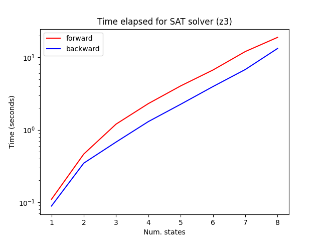
Figure 1: Time elapsed vs. size of true DFA for SMT encoding (Z3), $\eta=0$

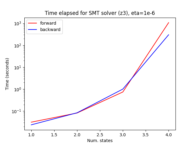
Figure 2: Time elapsed vs. size of true DFA for SMT encoding (Z3), $\eta=10^{-6}$

See Figure 1 and Figure 2 for plots of the time required by the Z3 solver versus the number of states in the underlying DFA for the exact learning and $\eta$-distance problems, respectively. The true language used for each data point is

$$L_{n}=\{x\in\Sigma^{*}\mid\sum_{i=1}^{|x|}\mathbf{1}\{x_{i}=1\}\equiv 0\mod n\}.$$ (8)

Note that the minimal automaton for $L_{n}$ has exactly $n$ states. For this experiment, the example set $\Sigma^{\leq k}$ was chosen such that $k$ is a constant larger than the size $n$ of the largest DFA used. From the plots, it is apparent that, for the exact learning problem, the time elapsed grows exponentially in the number of states. For the $\eta$-distance problem, the time seems to grow super-exponentially.

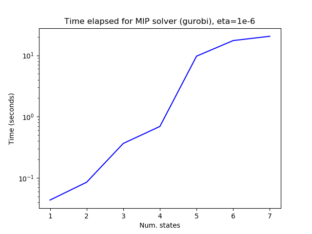
Figure 3: Time elapsed vs. size of true DFA (Gurobi), $\eta=10^{-6}$

We also ran the same time-versus-size experiment for the MIP program, using the Gurobi solver [12]; see Figure 3. Since the encoding is formed from the conjunction of several matrix-multiplication constraints, it is intuitively reasonable that a MIP optimizer may perform better than an SMT solver. The experiments confirm this to be the case: as seen in Figure 2, the Gurobi solver finds the minimal automaton in significantly less time. However, the plot also shows that the time elapsed still grows roughly exponentially with the true number of states.

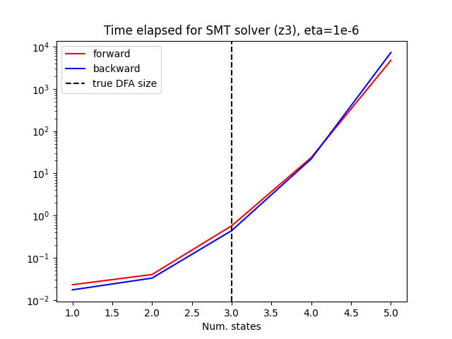
Figure 4: Time elapsed vs. size of SMT encoding (Z3), $\eta=10^{-6}$

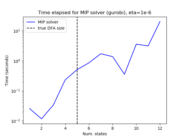
Figure 5: Time elapsed vs. size of SMT encoding (Gurobi), $\eta=10^{-6}$

Another reasonable hypothesis is that the time required to solve either the SMT or MIP encoding peaks when the size of the encoding is equal to the size of the true minimal DFA. This is supported by the intuition that there are many more DFAs of size greater than minimum, and thus the larger encodings might be less-constrained, with far more satisfying solutions. However, as our experiments show (see Figure 4 and Figure 5 for the SMT and MIP encodings, respectively), this intuition does not apply —the time required by the solver continues to grow exponentially with the size of the encoding, even though the size of the true DFA was fixed to a constant size. This is true for both the SMT and MIP encodings.

4 Conclusion

In this report, we covered a polynomial-time algorithm based on the concept of $\varepsilon$-closure, which turns out to output hypotheses with exponentially-bad error. We also examined SMT and MIP encodings of the same problem. For these encodings, the output is guaranteed to be close to the input oracle since it is constrained to be so. However, there is no guarantee of an efficient running time, and indeed the time required by both the SMT solver and MIP optimizer empirically appeared to grow exponentially with the size of the true minimal DFA. At least qualitatively, this provides some evidence that the problem of learning minimal DFAs within an $\eta$-distance of confidence oracles may be computationally hard.

Thus, a prudent next step would be to more carefully examine the complexity of the optimization problem (1). Although finding an exact solution (either deterministically or with high probability) intuitively seems difficult, we do not yet have any rigorous hardness result. Assuming in the future we do show this problem is $\NP$-hard, another question we can examine is the hardness of approximation. That is, we are interested in the bicriteria approximation problem of finding a DFA that is close in size to the solution of (1), while being e.g. a constant factor $c\eta$ away from the input oracle. It is not yet clear what approximation ratios can be achieved for these two criteria, or whether there is a way of trading off between size and distance. Note that the $\varepsilon$-closure algorithm already provides one weak positive result in this direction: it is possible to achieve optimal size with exponential approximation factor for distance.

Aside from complexity-theoretic concerns, we would also like to solve this problem in practice, for the reasons listed in Section 1.1. In this vein, we have not yet shown for certain that our SMT and MIP encodings are impractical. We have only run experiments on the “mod” language family described described in Equation 8; it is possible that these are particularly difficult languages to learn. Since most languages found in practice are not of the “mod” family, it is worthwhile to experiment on other languages, for example Tomita grammars or random DFAs.

Furthermore, there might be some way of combining the $\varepsilon$-closure and SMT approaches to achieve a decent approximation in a practical amount of time. For example, the SMT solver could be fed information from a partial hypothesis by the $\varepsilon$-closure algorithm in order to reduce the search space. Along with this, the SMT solver may be able to provide symbolic counterexamples that are useful to the $\varepsilon$-closure algorithm. Further investigation is necessary to determine if such an approach is useful in practice.

Finally, this project touches upon several of the topics covered in EECS 219C. The most immediate connection is the encoding of our problem in the form of an SMT formula over linear real arithmetic. The SMT solving techniques discussed in class are present in some form in the Z3 solver used for this project, along with many more advanced methods. Moreover, both Angluin’s $L^{*}$ algorithm for exact learning of DFA, as well as our $\varepsilon$-closure algorithm, can be considered instantiations of oracle-guided inductive synthesis (OGIS). Beyond this, the main connection to the course is within the motivation for this project. That is, the reason we wish to learn a finite automaton from the confidence oracle in the first place is because, as seen in class, there exist various model-checking techniques that work well on automata. Thus, given a confidence oracle in some abstract or cumbersome representation, it is useful to be able to replace it with a DFA that functions similarly, but is much easier to formally verify.

5 Acknowledgements

Thanks to Marcell Vazquez-Chanlatte and Sanjit Seshia.

Appendix A Proof of Proposition 1

Recall that we are considering the special case where $|Q|=(\lambda\Sigma)^{-|x|}$. We will first prove some helpful lemmas.

Lemma 1.

For any languages $L_{1},L_{2}\subseteq\Sigma^{*}$, and any strings $u,v\in\Sigma^{*}$, if $|u|\geq|v|$, then

$$d_{Q}(u^{-1}L_{2},v^{-1}L_{2})\leq 2(\lambda|\Sigma|)^{|u|}d_{Q}(L_{1},L_{2})+d_{Q}(u^{-1}L_{1}+v^{-1}L_{1}).$$

In particular, if $u^{-1}L_{1}=v^{-1}L_{1}$ then

$$d_{Q}(u^{-1}L_{2},v^{-1}L_{2})\leq 2(\lambda|\Sigma|)^{|u|}d_{Q}(L_{1},L_{2}).$$

Proof.

First, notice that

$$d_{Q}(L_{1},L_{2}) \geq\sum_{x\in\Sigma^{|u|}}\sum_{y\in\Sigma^{*}}(\lambda|\Sigma|)^{-|x\cdot y|}\mathbf{1}\{L_{1}(x\cdot y)\neq L_{2}(x\cdot y)\}$$

$$=\sum_{x\in\Sigma^{|u|}}(\lambda|\Sigma|)^{-|x|}\sum_{y\in\Sigma^{*}}(\lambda|\Sigma|)^{-|y|}\mathbf{1}\{L_{1}(x\cdot y)\neq L_{2}(x\cdot y)\}$$

$$=(\lambda|\Sigma|)^{-|u|}\sum_{x\in\Sigma^{|u|}}d_{Q}(x^{-1}L_{1},x^{-1}L_{2})$$

$$\geq(\lambda|\Sigma|)^{-|u|}d_{Q}(u^{-1}L_{1},u^{-1}L_{2}).$$

Rearranging, $d_{Q}(u^{-1}L_{1},u^{-1}L_{2})\leq(\lambda|\Sigma|)^{-|u|}d_{Q}(L_{1},L_{2})$.

Using the triangle inequality,

$$d_{Q}(u^{-1}L_{2},v^{-1}L_{2}) \leq d_{Q}(u^{-1}L_{2},u^{-1}L_{1})+d_{Q}(u^{-1}L_{1},v^{-1}L_{1})+d_{Q}(v^{-1}L_{1},v^{-1}L_{2})$$

$$\leq 2(\lambda|\Sigma|)^{|u|}d_{Q}(L_{1},L_{2})+d_{Q}(u^{-1}L_{1},v^{-1}L_{1}).$$

since by assumption $|u|\geq|v|$. ∎

Lemma 2.

Let $A$ and $A^{\prime}$ be two DFAs over the same set of states $S$, differing on only a single transition. That is, let $\delta$ and $\delta^{\prime}$ be the transition functions for $A$ and $A^{\prime}$ respectively. Then for some $t,s,s^{\prime}\in S$, and $\sigma\in\Sigma$, we have $\delta(t,\sigma)=s$ while $\delta(t,\sigma)=s^{\prime}$, and otherwise $\delta$ and $\delta^{\prime}$ agree. Let $u,u^{\prime}\in\Sigma^{*}$ be access strings to $s,s^{\prime}$ respectively, and let $v\in\Sigma^{*}$ be the shortest access string to $t$. Then,

$$d_{Q}(A,A^{\prime})\leq(\lambda^{-1}-1)^{-1}\lambda^{-|v|}d_{Q}(u^{-1}A,(u^{\prime})^{-1}A).$$

Proof.

Let $S_{t}$ be the set of all minimal access strings to $t$, in the sense that no prefix of any $x\in S_{t}$ is also an access string to $t$. Then,

$$d_{Q}(A,A^{\prime}) =\sum_{x\in S_{t}}\sum_{y\in\Sigma^{*}}(\lambda|\Sigma|)^{-|x\cdot\sigma\cdot y|}\mathbf{1}\{A(x\cdot\sigma\cdot y)\neq A^{\prime}(x\cdot\sigma\cdot y)\}$$

$$=\sum_{x\in S_{t}}\sum_{y\in\Sigma^{*}}(\lambda|\Sigma|)^{-|x\cdot\sigma\cdot y|}\mathbf{1}\{u^{-1}A(y)\neq(u^{\prime})^{-1}A^{\prime}(y)\}$$

$$=\sum_{x\in S_{t}}(\lambda|\Sigma|)^{-(|x|+1)}d_{Q}(u^{-1}A,(u^{\prime})^{-1}A^{\prime})$$

$$\leq\sum_{k=|v|}^{\infty}\sum_{x\in\Sigma^{k}}(\lambda|\Sigma|)^{-(k+1)}d_{Q}(u^{-1}A,(u^{\prime})^{-1}A^{\prime})$$

$$\leq\sum_{k=|v|}^{\infty}(\lambda)^{-(k+1)}d_{Q}(u^{-1}A,(u^{\prime})^{-1}A^{\prime})$$

$$\leq(\lambda^{-1}-1)^{-1}\lambda^{-|v|}d_{Q}(u^{-1}A,(u^{\prime})^{-1}A^{\prime}).$$

∎

Proof of Proposition 1.

Recall that we define $A^{*}$ to be the minimal automaton such that

$$d_{Q}(A^{*},L_{Q})\leq\eta.$$

We observe that the algorithm performs a BFS traversal of a subset of the states of $A^{*}$. This is due to the choice of $\varepsilon=2(\lambda|\Sigma|)^{|u|}\eta$ when exploring the state accessed by $u\in\Sigma^{*}$. That is, the algorithm only adds a new state $v$ to $S$ if

$$d_{Q}(u^{-1}L_{Q},v^{-1}L_{Q})\geq 2(\lambda|\Sigma|)^{|u|}\eta\geq 2(\lambda|\Sigma|)^{|u|}d_{Q}(A^{*},L_{Q}).$$

By Lemma 1, this can only occur if $d_{Q}(u^{-1}A^{*},v^{-1}A^{*})>0$; i.e., the strings $u$ and $v$ access distinct states in the minimal automaton $A^{*}$. Therefore, the $\varepsilon$-closure algorithm never adds extraneous states to $S$; the access strings in the queue represent a subset of the states of $A^{*}$, without duplicates. The fact that this subset is traversed in BFS order is simply due to the fact that $S$ implemented as a queue—since this is the case, we know that each string in $S$ is in fact the shortest access string to a particular state.

However, it is possible that the transition assigned by the $\varepsilon$-closure algorithm is incorrect; that is, while exploring the $\sigma$-transition of some state $t$, instead of assigning the correct next state $s$, we instead assign some other state $s^{\prime}$ of $A^{*}$. Let $v\in\Sigma^{*}$ be the access string in $S$ corresponding to $t$ that we are exploring; by the BFS traversal we know that $v$ is the shortest string accessing $t$. Let $u,u^{\prime}\in\Sigma^{*}$ be access strings to the states $s$ and $s^{\prime}$, respectively. By the definition of the $\varepsilon$-closure algorithm, we know that

$$d_{Q}(u^{-1}L_{Q},(u^{\prime})^{-1}L_{Q})\leq\varepsilon=2(\lambda|\Sigma|)^{|v|}\eta.$$

By Lemma 1, this can only occur if

$$d_{Q}(u^{-1}A^{*},(u^{\prime})^{-1}A*)\leq 2(\lambda|\Sigma|)^{|u|}d_{Q}(A^{*},L_{Q})+\varepsilon\leq 4(\lambda|\Sigma|)^{|u|}\eta.$$

The idea now is that whenever the algorithm mistakenly assigns a transition to $s$ instead of $s^{\prime}$, we know that the two states are not too far apart in the true automaton $A^{*}$. Since our hypothesis automaton $A$ will have the same set of states as $A^{*}$, with some number of incorrect transitions, we can use Lemma 2 to bound the distance from $A$ to $A^{*}$ (and thus $d_{Q}(A,L_{Q})$, by triangle inequality). More precisely, let us think of the $A$ as the result of a sequence of no more than $|\Sigma|n$ mistakes (since there are only this many transitions in $A^{*}$); this corresponds to a sequence of automata $A^{(1)},\ldots,A^{(k)}$ on the same states where $A^{(1)}=A$ is the true automaton and $A^{(k)}=A$ is our hypothesis, and each consecutive pair $A^{(j)},A^{(j+1)}$ differs on exactly one transition. That is, letting $\delta^{(j)}$ and $\delta^{(j+1)}$ be the transition functions for $A^{(j)}$ and $A^{(j+1)}$ respectively, we have for some states $t_{j},s_{j},s^{\prime}_{j}$ and $\sigma_{j}\in\Sigma$ that

$$\delta^{(j)}(t_{j},\sigma_{j})=s_{j}$$

while

$$\delta^{(j+1)}(t_{j},\sigma_{j})=s^{\prime}_{j}.$$

By Lemma 1,

$$d_{Q}(s_{j+1}^{-1}A^{(j+1)},(s^{\prime}_{j+1})^{-1}A^{(j+1)}) \leq 2(\lambda|\Sigma|)^{n}d_{Q}(A^{(j)},A^{(j+1)})+d_{Q}(s_{j+1}^{-1}A^{*},(s^{\prime}_{j+1})^{-1}A^{*})$$

$$\leq 2(\lambda|\Sigma|)^{n}d_{Q}(A^{(j)},A^{(j+1)})+4(\lambda|\Sigma|)^{n}\eta.$$

By Lemma 2,

$$d_{Q}(A^{(j)},A^{(j+1)})\leq(\lambda^{-1}-1)^{-1}d_{Q}(s_{j}^{-1}A^{(j)},(s^{\prime}_{j})^{-1}A^{(j)})$$

(we drop the $\lambda^{|s_{j}|}$ term, which is less than one.) Thus, we have the recurrence

$$d_{Q}(A^{(j)},A^{(j+1)})\leq 2(\lambda^{-1}-1)(\lambda|\Sigma|)^{n}d_{Q}(A^{(j-1)},A^{(j)})+4(\lambda|\Sigma|)^{n}.$$

Unraveling this recurrence using the triangle inequality and the fact that $k\leq|\Sigma|n$, we have

$$d_{Q}(A^{*},A)=d_{Q}(A^{(1)},A^{(k)})\leq(\lambda|\Sigma|)^{O(|\Sigma|n^{2})}\eta$$

as desired.

Note that the $\varepsilon$-closure algorithm provides only the transition topology of $A$, but once this is known it is not difficult to learn the accepting states with only $O(\eta)$ additional error. ∎

Admittedly, the bounds in the proof are fairly crude. However, even with a more refined analysis, the exponential term remains.

References

- [1] R. Pascanu, T. Mikolov, and Y. Bengio, “On the difficulty of training recurrent neural networks,” in Proceedings of the 30th International Conference on International Conference on Machine Learning - Volume 28, ICML’13, p. III–1310–III–1318, JMLR.org, 2013.
- [2] D. Angluin, “Learning regular sets from queries and counterexamples,” Information and Computation, vol. 75, pp. 87–106, 11 1987.
- [3] M. Kearns and L. Valiant, “Cryptographic limitations on learning boolean formulae and finite automata,” Journal of the ACM, vol. 41, pp. 67–95, 1 1994.
- [4] E. M. Gold, “Complexity of automaton identification from given data,” Information and Control, vol. 37, pp. 302–320, 6 1978.
- [5] L. Pitt and M. K. Warmuth, “The minimum consistent DFA problem cannot be approximated within any polynomial,” J. ACM, vol. 40, p. 95–142, Jan. 1993.
- [6] G. Weiss, Y. Goldberg, and E. Yahav, “Extracting automata from recurrent neural networks using queries and counterexamples,” in Proceedings of the 35th International Conference on Machine Learning (J. Dy and A. Krause, eds.), vol. 80 of Proceedings of Machine Learning Research, (Stockholmsmässan, Stockholm Sweden), pp. 5247–5256, PMLR, 10–15 Jul 2018.
- [7] Q. Wang, K. Zhang, A. G. Ororbia, X. Xing, X. Liu, and C. L. Giles, “An empirical evaluation of rule extraction from recurrent neural networks,” Neural Comput., vol. 30, pp. 2568–2591, Sept. 2018.
- [8] B. Balle, X. Carreras, F. M. Luque, and A. Quattoni, “Spectral learning of weighted automata: A forward-backward perspective,” Machine Learning, vol. 96, pp. 33–63, 10 2014.
- [9] A. Nerode, “Linear automaton transformations,” Proceedings of the American Mathematical Society, vol. 9, pp. 541–541, apr 1958.
- [10] M. J. H. Heule and S. Verwer, “Exact DFA identification using SAT solvers,” in Grammatical Inference: Theoretical Results and Applications (J. M. Sempere and P. García, eds.), (Berlin, Heidelberg), pp. 66–79, Springer Berlin Heidelberg, 2010.
- [11] L. De Moura and N. Bjørner, “Z3: An efficient smt solver,” in Proceedings of the Theory and Practice of Software, 14th International Conference on Tools and Algorithms for the Construction and Analysis of Systems, TACAS’08/ETAPS’08, (Berlin, Heidelberg), p. 337–340, Springer-Verlag, 2008.
- [12] L. Gurobi Optimization, “Gurobi optimizer reference manual,” 2020.