Gradients and frequency profiles of quantum re-uploading models

Abstract

Quantum re-uploading models have been extensively investigated as a form of machine learning within the context of variational quantum algorithms. Their trainability and expressivity are not yet fully understood and are critical to their performance. In this work, we address trainability through the lens of the magnitude of the gradients of the cost function. We prove bounds for the differences between gradients of the better-studied data-less parameterized quantum circuits and re-uploading models. We coin the concept of absorption witness to quantify such difference. For the expressivity, we prove that quantum re-uploading models output functions with vanishing high-frequency components and upper-bounded derivatives with respect to data. As a consequence, such functions present limited sensitivity to fine details, which protects against overfitting. We performed numerical experiments extending the theoretical results to more relaxed and realistic conditions. Overall, future designs of quantum re-uploading models will benefit from the strengthened knowledge delivered by the uncovering of absorption witnesses and vanishing high frequencies.

I Introduction

Variational Quantum Algorithms (VQAs) have emerged as a prominent paradigm in the realm of quantum computing as a hybrid computational model suited for NISQ (Noisy Intermediate-Scale Quantum) Preskill (2018) devices in conjunction with classical optimization techniques Bharti et al. (2022); Cerezo et al. (2021a). These algorithms rely on the minimization of cost functions McClean et al. (2021); Bittel and Kliesch (2021), which encode specific computational problems. VQAs have been used to solve a variety of problems, including approximating ground states Peruzzo et al. (2014); McClean et al. (2016); Ryabinkin et al. (2019), combinatorial challenges Farhi et al. (2014), chemistry problems Cao et al. (2019), quantum simulation McArdle et al. (2019); Yuan et al. (2019) and simulation of quantum systems Li and Benjamin (2017); Cirstoiu et al. (2020); Bharti and Haug (2021). Furthermore, VQAs have served as quantum computing engines for tackling various machine learning (ML) tasks, such as function regression Mitarai et al. (2018); Schuld et al. (2020), classification Havlíček et al. (2019); Schuld (2021); Otterbach et al. (2017) or generative models Zoufal et al. (2019, 2021); Dallaire-Demers and Killoran (2018). We specifically make a distinction between linear models on the one side, introducing data either as input states or through encoding maps Schuld and Killoran (2019), and quantum re-uploading (QRU) schemes on the other side, which introduce data iteratively throughout the execution of the quantum circuit Vidal and Theis (2020); Schuld et al. (2021); Pérez-Salinas et al. (2020, 2021a).

The performance of VQAs hinges on two critical properties: expressivity and trainability. Expressivity embodies the model’s ability to represent precise solutions to the underlying problem, while trainability is a measure of the difficulty in finding the parameter set that yields the optimal attainable solution within the model. In the case of data-independent VQAs, expressivity can be intuitively understood as the proportion of attainable output states within the Hilbert space Sim et al. (2019). In the context of data-dependent ML, expressivity pertains to the suitability of the output function in fitting the data Cybenko (1989); Hornik (1991). The universality of QRU models has been proven even with a single qubit Schuld et al. (2021); Pérez-Salinas et al. (2021b). Trainability in VQAs, on the other hand, is closely linked to characteristics of the cost function, such as non-convexity Anschuetz and Kiani (2022) or vanishing gradients McClean et al. (2018). The relationship between the trainability of VQAs and QML schemes without re-uploading has also been previously studied Thanasilp et al. (2023). Importantly, trainability and expressivity are usually mutually exclusive. In particular, for VQAs there exists a well-studied trade-off between these two properties Holmes et al. (2022); Hubregtsen et al. (2021).

In this work, we specifically explore QRU models with a focus on exploring trainability and expressivity. Our investigation into trainability focuses on the on-average behavior of gradients, which can be related to the flatness of the cost function. We compare the cost functions of QRU models and base PQCs, which are circuits with the same architecture and observable as the QRU, but where the data gates are removed. The difference between the flatness of both cost functions is upper bounded by a quantity we refer to as absorption witness, which quantifies the influence of data gates on the quantum circuit when averaged over the parameter space. Such derivation opens a path to transfer existing knowledge about the flatness of PQCs McClean et al. (2018); Larocca et al. (2022, 2021) to guide the design of QRU models.

The second segment of our findings is related to the expressivity of data-dependent output functions generated by QRU models. It is known that any hypothesis function output by QRU models can be expressed as a generalized trigonometric polynomial, with the range of available frequencies contingent on the data encoding scheme Caro et al. (2021); Schuld et al. (2021). We show that, under reasonable assumptions, the average magnitude of individual frequency components in the hypothesis function rapidly tends to a Gaussian profile, with a variance scaling as $\sim\sqrt{L}$, with $L$ being the number of re-uploading steps, while the support in frequencies scales as $\sim L$. This property inherently biases the attainable hypothesis functions as being dominated by lower-frequency components. This has a direct consequence on the Lipschitz constants of these output functions.

The paper is organized as follows.  Section II introduces relevant concepts and notation for the paper. Section III delves into the expected norm of gradients in QRU models. Section IV delves into the expressive capabilities of output functions within QRU models in terms of spectrum. Section V showcases numerical experiments that substantiate our theoretical findings.  Section VI engages in a discussion of the implications and potential avenues opened up by our research. Conclusions are summarized in Section VII.

II Background

In this work, we refer to a PQC as a sequence of parameterized gates and fixed gates applied to an initial state, namely

$$U({\bm{\theta}})=\prod_{j=1}^{M}\ W_{j}e^{iV_{j}\theta_{i}},$$ (1)

where $\{V_{j}\}$ are, without loss of generality, traceless Hermitian matrices known as generators, $\{W_{j}\}_{j=1}^{M}$ are fixed unitary operations, and ${\bm{\theta}}\in{\bm{\Theta}}\subset\mathbb{R}^{M}$. We use these PQCs as a baseline for QRU models Pérez-Salinas et al. (2020, 2021b); Schuld et al. (2021). This model consists of a PQC where data-encoding gates have been added in the form

$$U({\bm{\theta}},x)=\prod_{j=1}^{M}\ e^{ig_{j}x}\ W_{j}e^{iV_{j}\theta_{i}},$$ (2)

where $\{g_{j}\}_{j=1}^{M}$ are, without loss of generality, traceless Hermitian generators. We do not impose constraints in $\{V_{j}\}\cap\{g_{j}\}$. The input $x$ is a real number. Extensions to multidimensional values of $x$ are available by adding extra terms to the model, although this case will not be considered in this work. Notice that there exists a mapping between PQCs with data as initial state and QRU models, thus making both computations formally equivalent Jerbi et al. (2023), up to overheads.

QRU models yield ${\bm{\theta}}$-dependent hypothesis functions

$$h_{\bm{\theta}}(x)=\bra{0}U^{\dagger}({\bm{\theta}},x)HU({\bm{\theta}},x)\ket{0},$$ (3)

when applied to an initial quantum state and measured with an observable $H$. Notice that $h_{\bm{\theta}}(x=x_{0})$ for a fixed value $x_{0}$ is the standard definition of the cost function of a PQC. In the case $x_{0}\neq 0$, we can recover our formulation of PQC by adapting the fixed gates $W_{j}$. The values of ${\bm{\theta}}$ are trainable to match data coming in pairs $X=\{(x,y(x)\}$, such that $h_{\bm{\theta}}(x)\approx y(x)$. These hypothesis functions can be expressed as a generalized trigonometric polynomial  Schuld et al. (2021); Caro et al. (2021), namely

$$h_{\bm{\theta}}(x)=\sum_{\omega\in\Omega}a_{\omega}({\bm{\theta}})e^{i\omega x},$$ (4)

where $a_{\omega}({\bm{\theta}})=a_{-\omega}^{*}({\bm{\theta}})$ to ensure real valued hypothesis functions, and $\Omega$ is the set of available frequencies.

The training of VQAs involves an optimization procedure where a parameter set minimizing a cost function is searched. The difficulty of this optimization task is enclosed under the broad concept of trainability. A paradigmatic example of optimizing a PQC is minimizing $h_{\bm{\theta}}(x=0)$ with respect to ${\bm{\theta}}$ to find an approximation to the ground state of the corresponding Hamiltonian $H$. Trainability has been extensively studied in the context of PQCs Anschuetz and Kiani (2022); McClean et al. (2018). Training a QRU model involves finding the optimal set of parameters ${\bm{\theta}}$ for which $h_{\bm{\theta}}(x)$ approximately matches some target function given by data. Trainability may depend on several features of the cost function landscape Muñoz et al. (2015), such as small gradients Pascanu et al. (2013) or non-convexity, e.g. the existence of (many) local minima Friedrich et al. (2022). In this work, we focus on average behaviors of gradients of the cost function, inspired by the well-studied phenomenon of vanishing gradients barren plateaus (BP) McClean et al. (2018); Cerezo et al. (2021a); Holmes et al. (2022).

Expressivity is another crucial aspect of parameterized models, capturing their ability to represent various solutions. For PQCs, expressivity entails the existence of parameter sets ${\bm{\theta}}^{*}$ making $U({\bm{\theta}}^{*},0)$ close to some unitary operations $V\in\mathcal{SU}(2^{n})$, within a specified tolerance and respect to some distance. Expressivity is often measured relative to unitary $t$-designs Sim et al. (2019). In contrast, expressivity in the context of ML (e.g. QRU models) is related to the output function and its capability. A model is expressive if its output is able to match a variety of target functions to fit some data Raghu et al. (2017).

III Gradients in QRU models

In this section, we focus on characterizing gradients of QRU models, as compared to those of PQCs. In the case of PQC, the gradients of interest are typically defined in relationship to their cost function $h_{\bm{\theta}}(0)$. However, the optimization of QRU models involves a cost function that depends on both the quantum circuit, expressed through $h_{\bm{\theta}}(x)$, and the available data, provided in pairs as $(x,y(x))$. Such cost function is usually given by averaging a distance between functions $\Delta(\cdot,\cdot)$ as

$$\mathcal{L}_{X}({\bm{\theta}})=\mathbb{E}_{X}\left(\Delta(h_{\bm{\theta}}(x),y(x))\right),$$ (5)

where $\mathbb{E}_{X}\left(\cdot\right)$ denotes expectation value over the training dataset $X=\{(x,y(x))\}$, usually composed by a discrete set of points. Notice that $\mathcal{L}_{X}$ is empirical as the training dataset is drawn from an unknown data distribution $X\sim\mathcal{D}$, and approximates the true unaccessible risk averaged over $\mathcal{D}$. A common choice for the distance metric $\Delta(\cdot,\cdot)$ is the mean squared error.

Our interest lies in examining the gradients of the loss function, expressed as

$$\partial_{j}\mathcal{L}({\bm{\theta}})=\mathbb{E}_{X}\left(\frac{\partial\Delta(h_{\bm{\theta}}(x),y(x))}{\partial h_{\bm{\theta}}(x)}\partial_{j}h_{\bm{\theta}}(x)\right).$$ (6)

For the purpose of our investigation, we focus solely on the effect of QRU models. The influence imposed by the choice of distance function $\Delta(\cdot,\cdot)$ can be readily bounded e. g. using its Lipschitz constant $L_{\Delta}$. In particular,

$$\operatorname{Var}_{{\bm{\Theta}}}\left(\partial_{j}\mathcal{L}({\bm{\theta}})\right)\leq L_{\Delta}^{2}\operatorname{Var}_{{\bm{\Theta}}}\left(\mathbb{E}_{X}\left(\partial_{j}h_{\bm{\theta}}(x)\right)\right).$$ (7)

Therefore, we can bound vanishing gradients by studying only $\operatorname{Var}_{{\bm{\Theta}}}\left(\mathbb{E}_{X}\left(\partial_{j}h_{\bm{\theta}}(x)\right)\right)$.

We connect now the gradients of loss functions for QRU models and PQCs. First, the average of derivatives of hypothesis functions are zero, namely Holmes et al. (2022)

$$\mathbb{E}_{{\bm{\Theta}}}\left(\mathbb{E}_{X}\left(\partial_{j}h_{\bm{\theta}}(x)\right)\right)=\mathbb{E}_{X}\left(\mathbb{E}_{{\bm{\Theta}}}\left(\partial_{j}h_{\bm{\theta}}(x)\right)\right)=0,$$ (8)

if the parameters ${\bm{\theta}}$ are sampled uniformly from ${\bm{\Theta}}$. As a consequence, due to the convexity of the square function, we have $\mathbb{E}\left(x\right)^{2}\leq\mathbb{E}\left(x^{2}\right)$. By combining these two observations and the definition $\operatorname{Var}\left(x\right)=\mathbb{E}\left(x^{2}\right)-\mathbb{E}\left(x\right)^{2}$, we derive

$$\operatorname{Var}_{{\bm{\Theta}}}\left(\mathbb{E}_{X}\left(\partial_{j}h_{\bm{\theta}}(x)\right)\right)\leq\mathbb{E}_{X}\left(\operatorname{Var}_{{\bm{\Theta}}}\left(\partial_{j}h_{\bm{\theta}}(x)\right)\right),$$ (9)

which can be readily connected to $\operatorname{Var}_{{\bm{\Theta}}}\left(\partial_{j}\mathcal{L}({\bm{\theta}})\right)$ via Equation 7. Therefore, we can bound the variance of cost functions in QRU by the average of variances cost functions of several PQC, defined by different fixed $x_{0}$. Bounds on $\operatorname{Var}_{{\bm{\Theta}}}\left(\partial_{j}h_{\bm{\theta}}(0)\right)$ have been studied in the context of PQC. In particular, BPs are defined for exponentially vanishing bounds to $\operatorname{Var}_{{\bm{\Theta}}}\left(\partial_{j}h_{\bm{\theta}}(0)\right)$ McClean et al. (2018).

Equation 9 suggests that QRU models present vanishing gradients if the base PQC presents BPs, which means that it is recommendable to use architectures that avoid vanishing gradients such as in Larocca et al. (2021); Schatzki et al. (2022) when designing QRUs. However, Equation 9 does not guarantee non-vanishing gradients for QRU models derived from BP-free PQCs. As an example, consider a re-uploading model with parameterized single-qubit gates and data-encoding entangling gates arranged in an alternate-layered structure, measured by a sum of 1-local observables, as illustrated in Figure 1, base PQC 1. A compatible base PQC is composed only of single-qubit parameterized gates. In this case, $h_{\bm{\theta}}(x_{0})$ from the base PQC has large gradients Cerezo et al. (2021b). The inclusion of data increases the accessible Hilbert space due to the presence of entangling operations, entanglement, which causes BPs Holmes et al. (2022).

Re-uploading  
[row sep=0.1cm, column sep=0.2cm] $\ket{0}$ & U 1 U X R_z(x) $\cdots$
$\ket{0}$ U X R_z(x) U 2 $\cdots$
$\vdots$
$\ket{0}$ U 1 U X R_z(x) $\cdots$
$\ket{0}$ U X R_z(x) U -4 $\cdots$
           Base PQC 1                   Base PQC 2                
[row sep=0.1cm, column sep=0.1cm] $\ket{0}$ & U U $\cdots$
$\ket{0}$ U U $\cdots$
$\vdots$
$\ket{0}$ U U $\cdots$
$\ket{0}$ U U $\cdots$ [row sep=0.1cm, column sep=0.1cm] $\ket{0}$ & U 1 U $\cdots$
$\ket{0}$ U U 2 $\cdots$
$\vdots$
$\ket{0}$ U 1 U $\cdots$
$\ket{0}$ U U -4 $\cdots$

Figure 1: Quantum circuits for the first experiments. The re-uploading model is depicted on top, and compared to the PQCs described in the bottom line. The $U$ gates here described correspond to arbitrary parameterized single-qubit operations. The circuit here described corresponds to one layer, and the depth is determined by the number of repetitions.

Consider again the previous example, this time with a different base PQC which includes entangling gates, see Figure 1, base PQC 2. In this new scenario, the PQC cost function $h_{\bm{\theta}}(0)$ suffers from BPs for sufficient depth Holmes et al. (2022); Cerezo et al. (2021b). Notice that it is possible to decompose a data-dependent entangling gate as a fixed entangling gate and tunable single-qubit Barenco et al. (1995), allowing for introducing data through single-qubit operations. Intuitively, the data can be re-absorbed by the parameters to generate a new circuit with the same ansatz as the base PQC. As a direct consequence, the gradients of the PQC and those of the QRU are of the same magnitude, $\mathbb{E}_{X}\left(\operatorname{Var}_{{\bm{\Theta}}}\left(\partial_{j}h_{\bm{\theta}}(x)\right)\right)\approx\operatorname{Var}_{{\bm{\Theta}}}\left(\partial_{j}h_{\bm{\theta}}(x_{0})\right)$, for any $x_{0}$. This intuition motivates the newly coined concept of absorption witnesses in Definition III.1 as the capability of the circuit to absorb the data into the parameters.

Before further expanding on absorption witnesses, it is convenient to introduce some auxiliary quantities in the context of QRU models. We take derivatives with respect to the $j$-th parameter. All operations preceding the $j$-th parameter (not included) are considered the right part of the circuit, operationally attached to the input state $\rho_{0}$. Operations that include and follow the $j$-th parameter are on the left side of the circuit, attached to the observable. This description is given by

$$\rho_{j}({\bm{\theta}}_{R,j},x) =U_{R,j}({\bm{\theta}}_{R,j},x)\ \rho_{0}\ U^{\dagger}_{R,j}({\bm{\theta}}_{R,j},x)$$ (10)

$$H_{j}({\bm{\theta}}_{L,j},x) =U^{\dagger}_{L,j}({\bm{\theta}}_{L,j},x)\ H\ U_{L,j}({\bm{\theta}}_{L,j},x).$$ (11)

The left/right parameters ${\bm{\Theta}}_{R/L,j}$ are assumed to be independent. For each of the right and left parts of the circuit, we can define the difference with respect to the reference data value $x=0$ (corresponding to the PQC) as

$$B_{R,j}^{(t)}({\bm{\theta}}_{R,j},x;\rho_{0}) =\rho_{j}^{\otimes t}({\bm{\theta}}_{R,j},x)-\rho_{j}^{\otimes t}({\bm{\theta}}_{R,j},0)$$ (12)

$$B_{L,j}^{(t)}({\bm{\theta}}_{L,j},x;H) =H_{j}^{\otimes t}({\bm{\theta}}_{L,j},x)-H_{j}^{\otimes t}({\bm{\theta}}_{L,j},0)$$ (13)

We define the absorption witness as follows.

Definition III.1 (Absorption witness).

Let $U({\bm{\theta}},x)$ be a re-uploading model as defined in Equation 2. Let $U_{R/L,j}({\bm{\theta}},x)$ be the right and left parts of the circuit with respect to the $j$-th gate. The right/left absorption witnesses are

$$\mathcal{B}^{(2)}_{R,j}(\rho_{0})= \mathbb{E}_{X}\left(\ \norm{\mathbb{E}_{{\bm{\Theta}}_{R,j}}\left(B^{(2)}_{R,j}({\bm{\theta}}_{R,j},x;\rho_{0})\right)}_{2}\right),$$ (14)

$$\mathcal{B}^{(2)}_{L,j}(H)= \mathbb{E}_{X}\left(\ \norm{\mathbb{E}_{{\bm{\Theta}}_{L,j}}\left(B^{(2)}_{L,j}({\bm{\theta}}_{L,j},x;H)\right)}_{2}\right).$$ (15)

The absorption witness defined above captures the effect of including data when averaging over the parameter space ${\bm{\Theta}}$. If $\mathcal{B}^{(2)}_{R,j}(\rho_{0})=0$, the input $x$ yields an effect on $\rho_{j}({\bm{\theta}}_{R,j},x)$ equivalent to some change ${\bm{\theta}}_{R,j}\rightarrow{\bm{\theta}}^{*}_{R,j}$. This effect is compensated when averaging over ${\bm{\Theta}}$. The logic is analogous to the left part of the circuit. As an illustrative example, assume a single-layer re-uploading model composed by applying any data-encoding layer after a PQC forming a $t$-design. By definition, $t$-designs approximate up to the $t$-th statistical moment of Haar measure and are thus insensitive (on average) to adding extra operations, in particular any operation given by data-encoding. However, this closeness to $t$-designs is no longer possible for ansatzes with (several) data-encoding gates interspersed between parameterized layers.

The absorption witnesses from Definition III.1 bound the differences between variances for PQCs and QRU models as follows.

Theorem III.1.

Let $U({\bm{\theta}},x)$ be a re-uploading model as defined in Equation 2. Then

$$|\mathbb{E}_{X}\left(\operatorname{Var}_{{\bm{\Theta}}}\left(\partial_{j}h_{\bm{\theta}}(x)\right)\right)-\operatorname{Var}_{{\bm{\Theta}}}\left(\partial_{j}h_{{\bm{\theta}}}(0)\right)|\\ \leq 4\norm{V_{j}}_{2}^{2}\left(\norm{H}_{2}^{2}\ \mathcal{B}^{(2)}_{R,j}(\rho_{0})+\ \norm{\rho_{0}}_{2}^{2}\ \mathcal{B}^{(2)}_{L,j}(H)\right)$$ (16)

where $\rho_{0}$ is the initial state, $H$ is the observable to measure, and $\mathcal{B}^{(2)}_{L,j}(H),\mathcal{B}^{(2)}_{R,j}(\rho_{0})$ are the absorption witnesses from Definition III.1.

The proof can be found in Section A.1.

Computing the absorption witness is not easy. However, it provides a useful interpretation of the relationship between vanishing gradients for data-dependent QRU models, as compared to their base PQCs, where the BP phenomenon has been already studied McClean et al. (2018); Larocca et al. (2022, 2021). This result is formulated in the same fashion as the ones in Holmes et al. (2022), extending their applicability to quantum machine learning. The result from Theorem III.1 admits further simplification when considering layered ansatzes, see Section III.1.

Finally, note that it is in principle possible to construct pathological datasets such that the base PQC suffers from BP while the QRU model does not. In these cases, the data uploading gates need a careful design to cancel out the structures responsible for vanishing gradients. It is thus reasonable to assume that real-world datasets would not result in such behavior.

III.1 Gradients in layered QRU models

We consider in this section layered QRU models. In many practical scenarios there are several parameterized gates between each pair of encoding gates Larocca et al. (2022, 2021). An encoding gate and all preceding parameterized gates is referred to as a layer as

$$U({\bm{\theta}},x)=\prod_{l=1}^{L}V_{l}(x)u_{l}({\bm{\theta}}_{l}).$$ (17)

In this representation, the parameterized gates $u({\bm{\theta}}_{l})$ are no longer defined by a single generator, and ${\bm{\theta}}_{l}$ is no longer one-dimensional. We can in this case study the absorption capability of each individual layer by defining the corresponding absorption witnesses as follows.

Definition III.2 (Layerwise absorption witness).

Let $u({\bm{\theta}}_{l})$ be the $l$-th layer of a re-uploading model from Equation 2, and let $V(x)$ be the data-encoding operation applied immediately after $u({\bm{\theta}}_{l})$. The absorption witness for the $l$-th layer is

$$\mathcal{A}_{l}^{(t)}=\mathbb{E}_{X}\left(\norm{\mathbb{E}_{{\bm{\Theta}}_{l}}\left(V_{l}(x)^{\otimes 2}u({\bm{\theta}}_{l})^{\otimes 2}-u_{l}({\bm{\theta}}_{l})^{\otimes 2}\right)}_{2}\right).$$ (18)

We provide some examples where $\mathcal{A}_{l}^{(t)}=0$. First, assume a data-encoding layer sharing the generator with the corresponding parameterized gates. In this case, we can read data-encoding as a simple shift of parameters ${\bm{\theta}}^{*}\rightarrow{\bm{\theta}}-x$ (recall that ${\bm{\theta}}$ is now multi-dimensional), and averages do not change as long as ${\bm{\theta}}$ is sampled uniformly. Another example is the case where the ansatz is composed by $k$-local $2$-designs located in consecutively alternated qubits, as in Cerezo et al. (2021b), where any $k$-local data-encoding gates can be re-absorbed by definition.

The use of layered ansatzes and layerwise absorption witnesses allows for further simplifications of Theorem III.1 by bounding the complete absorption witnesses.

Lemma III.1.

Consider a layered re-uploading model as in Equation 17. Then

$$\mathcal{B}^{(2)}_{R,l+1}(\rho_{0}) \leq\mathcal{B}^{(2)}_{R,l}(\rho_{0})+\norm{\rho_{0}}_{2}^{2}\mathcal{A}_{l+1}^{(2)}$$ (19)

$$\mathcal{B}^{(2)}_{L,l}(H) \leq\mathcal{B}^{(2)}_{L,l+1}(\rho_{0})+\norm{H}_{2}^{2}\mathcal{A}_{l}^{(2)}.$$ (20)

The proof can be found in Section A.2.

Consider now a layered circuit where $u_{l}(\cdot)=u_{k}(\cdot)$ for any pair $(l,k)$. The previous result can be further simplified since $\mathcal{A}_{l}^{(2)}=\mathcal{A}^{(2)}$ for all values of $l$. Therefore

Corollary III.1.

For a layered re-uploading model, the absorption witnesses of large parts of the circuits can be bounded by absorption witnesses of small pieces, by

$$\mathcal{B}^{(2)}_{R,l}(\rho_{0}) \leq L\norm{\rho_{0}}_{2}^{2}\mathcal{A}^{(2)},$$ (21)

$$\mathcal{B}^{(2)}_{L,l}(\rho_{0}) \leq L\norm{H}_{2}^{2}\mathcal{A}^{(2)}.$$ (22)

The proof follows by repeated application of Lemma III.1, together with the observation $\mathcal{B}^{(2)}_{R,l}(\rho_{0})=0$ if no data-encoding layer is considered in the absorption witness. We can therefore give a simplified bound for the results from Equation 16 in the case of layered ansatz as

$$|\mathbb{E}_{X}\left(\operatorname{Var}_{{\bm{\Theta}}}\left(\partial_{j}h_{\bm{\theta}}(x)\right)\right)-\operatorname{Var}_{{\bm{\Theta}}}\left(\partial_{j}h_{{\bm{\theta}}}(0)\right)|\\ \leq 8L\norm{V_{j}}_{2}^{2}\norm{H}_{2}^{2}\ \norm{\rho_{0}}_{2}^{2}\mathcal{A}^{(2)}.$$ (23)

The result from Equation 23 is more loose than Theorem III.1, but easier to compute, since it depends only on the layerwise absorption witness $\mathcal{A}^{(2)}$ corresponding to shallow circuits.

IV Expressivity in QRU models

The hypothesis class of QRU can always be expressed as a generalized trigonometric polynomial Caro et al. (2021), see Equation 4. In QRU models, the set of frequencies $\Omega$ is generated through the sequential Minkowski sum of the spectrum of the data encoding generators $\{\lambda_{j}\}_{j}$. In the general case, $\{\lambda_{j}\}_{j}$ consists of incommensurable real numbers, i. e. with non-rational ratios, and each new encoding step makes $\Omega$ combinatorially denser. In this section we first consider harmonic generators, i. e. with integer eigenvalues, and extend the results later to generic generators. As a main observation of this work, the behavior is similar in both cases.

IV.1 Harmonic representation of quantum states

In this section, we introduce a representation of QRU models based on the Fourier decomposition of the hypothesis function. Such representation is useful for subsequent analytical results. Starting from Equation 2 and assuming the generators $g_{i}$ possess an integer spectrum, we can express the state before measurement as

$$U({\bm{\theta}},x)\ket{0}=\sum_{k=-K}^{K}\sum_{j=1}^{2^{n}}c_{j,k}({\bm{\theta}})e^{i\mu kx}\ket{j}.$$ (24)

The coefficients $c_{j,k}$ form a matrix $\bm{C}\in\mathbb{C}^{2^{n}\times(2K+1)}$ that defines uniquely (up to a global phase) the output state of the re-uploading circuit before measurement. The matrix $\bm{C}$ depends only on the parameters ${\bm{\theta}}$ and the generators of the ansatz, but not on the data $x$. The value $K$ corresponds to the largest attainable frequency, namely the sum of the largest eigenvalue for each generator used in the circuit. The recipe to construct $\bm{C}$ from the description of the circuit is detailed in Section A.3. Notice this approach is not efficient from a computational point of view, since an extra dimension (frequency) is added to standard state vector simulation. This harmonic representation of QRU models simulator is available on Barthe and Pérez-Salinas (2023).

IV.2 Vanishing high frequencies in QRU models

Using the above representations and the intuition that adding a data encoding layer corresponds to a convolution operation with the data encoding generator spectrum as defined below in IV.1, we examine the properties of the amplitude of the coefficients as a function of the frequency. We begin by defining the spectrum kernel of a harmonic Hermitian matrix.

Definition IV.1 (Harmonic spectrum kernel).

Let $H$ be a $N\times N$ Hermitian matrix with integer eigenvalues $\{\lambda\}$ with multiplicities $m(\lambda)$. The spectrum kernel of $H$ is the vector

$$\mathcal{K}_{H}(k)=\left\{\begin{matrix}m(k\mu)/N&\textrm{if $k\mu\in\{\lambda\}$}\\ 0&{\rm Otherwise}\end{matrix}\right.,$$ (25)

where $\mu$ is the largest value in $\mathbb{R}$ compatible with this description.

This function simply maps the eigenvalues of a Hermitian matrix into the normalized dimensionality of the corresponding eigenspace. For readability, we will refer to the spectrum multiplicity function simply as the spectrum for the remainder of the paper.

In the case of layered QRU models, the spectra of their data-encoding generators and the number of layers $L$ directly determine the set of attainable frequencies. The maximum attainable frequency is bounded by $L\norm{g}_{2}$. We provide now some insight into how the coefficients are expected to behave.

Lemma IV.1 (Harmonic convolution).

Let $\ket{\psi_{\bm{\theta}}(x)}=U({\bm{\theta}},x)\ket{\psi_{0}}$ be the output state of a re-uploading model, with data-encoded through the generator set $\{g_{j}\}$, each with spectrum $\mathcal{K}_{g_{j}}$, encoded as in Equation 24. Assuming that each parameterized step is drawn from the Haar measure of unitaries, then

$$\sum_{j}\absolutevalue{c_{j,k}}^{2}=\operatorname{Dir}\left(\left(\mathcal{K}_{g_{1}}\ast\ldots\ast\mathcal{K}_{g_{j}}\ast\ldots\ast\mathcal{K}_{g_{L}}\right)(k)\right),$$ (26)

where $\operatorname{Dir}(\alpha_{1},\alpha_{2},\ldots)$ is the Dirichlet distribution Dirichlet (2008) and $\ast$ denotes the convolution.

The proof can be found in Section A.4. For completeness, we define convolution as

$$(f*g)(k)=\sum_{l=-\infty}^{\infty}f[k]g[l-k].$$ (27)

The previous result immediately implies the following.

Theorem IV.1 (Single-generator convolution).

Let $\ket{\psi_{\bm{\theta}}(x)}=U({\bm{\theta}},x)\ket{\psi_{0}}$ be the output state of a re-uploading model, with data-encoded through the generator $g$, with spectrum $\mathcal{K}_{g}$, encoded as in Equation 24. Assuming that each parameterized step is drawn from the Haar measure of unitaries, then

$$\sum_{j}\absolutevalue{c_{j,k}}^{2}=\operatorname{Dir}\left(\left(\mathcal{K}_{g}^{*L}\right)(m)\right),$$ (28)

where $(\cdot)^{*L}$ denotes the $L$-fold convolution.

The proof is immediate from extending Lemma IV.1.

Notice that, provided that the data generator is known, it is possible to classically store $\mathcal{K}_{g}^{*L}$ within memory of size $\mathcal{O}\left(L\norm{g}_{2}/\mu\right)$, with computational cost $\mathcal{O}\left((L\norm{g}_{2}/\mu)^{3}\right)$. This allows us to classically characterize the frequency profile prior to executing the QRU model in quantum hardware for harmonic generators with only polynomially many eigenvalues.

The previous theorem can be readily interpreted in the limit of large $L$ by virtue of the central limit theorem Billingsley (1995). The repeated convolution of any random variable with a variance of $\sigma$ and a probability distribution in the spaces $L^{1}$ and $L^{2}$, tends to a normal distribution in a weak sense. We can thus obtain the following result.

Corollary IV.1 (Vanishing high frequencies).

In the conditions of Theorem IV.1 and for large number of re-uploading $L$,

$$\lim_{L\rightarrow\infty}\sum_{j}\absolutevalue{c_{j,k}}^{2}\sim\operatorname{Dir}\left(\mathcal{N}\left(0,\sigma_{g}^{2}L\right)(k)\right),$$ (29)

where $\sigma_{g}$ is the standard deviation of the spectrum $\mathcal{K}_{g}$, and $\mathcal{N}(\mu,\sigma^{2})$ is the normal distribution.

This observation implies that tails of the distribution vanish exponentially for large frequencies and there is a concentration in the low-frequency terms as the magnitudes of high-frequency terms vanish. In asymptotic scaling the available spectrum reduces from $\norm{g}_{\lambda}^{2}L$ to $\sigma_{g}\sqrt{L}$.

The results from Theorem IV.1 and Corollary IV.1 can be extended to non-harmonic generators. For readability, we postpone this result until Section IV.4.

The previous discussion considers the effects of the spectrum on the internal state of the re-uploading model in its harmonic representation. We are however not interested in the state itself, but rather in $h_{\bm{\theta}}(x)$ measured as an expectation value of this internal state. The Fourier components $h_{\bm{\theta}}(x)$ satisfy the following corollary.

Corollary IV.2.

Let $\ket{\psi_{\bm{\theta}}(x)}$ be the output state of a re-uploading model, with a single data-encoding generator $g$ with spectrum $\mathcal{K}_{g}$. Let $h_{\bm{\theta}}(x)$ be the hypothesis function induced by the observable $H$ in the re-uploading model, as in Equation 3, and let $a_{k}({\bm{\theta}})$ be their corresponding Fourier coefficients as in Equation 4. In the conditions of Theorem IV.1, and for symmetric spectra $\mathcal{K}_{g}(k)=\mathcal{K}_{g}(-k)$,

$$\norm{H}_{\lambda}^{-2}\left|a_{k}({\bm{\theta}})\right|^{2} \leq p_{k}$$ (30)

$$p_{k} \sim\operatorname{Dir}(\mathcal{K}_{g}^{*2L}(k)),$$ (31)

where $p_{k}$ is a multidimensional probability distribution sampled from the Dirichlet distribution defined by the $L$-fold convoluted spectrum $\operatorname{Dir}(\mathcal{K}_{g}^{*2L}(k))$ Dirichlet (2008).

Additionally, this result extends to the Gaussian distribution in the limit of large $L$ as for Corollary IV.1.

The results from this section show that the frequency terms of $h_{\theta}(x)$ tend to follow a Gaussian profile of width $\sim L$. However, the frequency support of these functions scales linearly in $L$. As an immediate consequence, only frequencies $\omega\in\mathcal{O}(\sqrt{L})$ have practical support on average, while larger frequencies have exponentially vanishing weight in the hypothesis function. Note, that the Gaussian profile described by Corollary IV.1 does not imply a dense frequency space, which is still restricted to integer frequencies. This result holds even in the case where the generator provides exponentially-in-qubits many frequencies. It is then possible to have exponentially large frequency sets even with a small number of re-uploading steps, and the Gaussian approximation still holds with $\sigma\sim\sqrt{L}e^{n}$.

IV.3 Lipschtitz expressivity

In this section, we delve into a more practical understanding of the expressivity of hypothesis functions in terms of the magnitude of their derivatives. The ability to capture fine-grained data patterns depends on the function’s ability to access high rates of change, i.e., the magnitude of its derivative. This concept can be quantified through the maximum value of the derivative, known as the optimal Lipschitz constant. For a function $f$, the optimal Lipschitz constant is defined as

$$\mathcal{L}(f)={\rm max}_{x}\left|\partial_{x}f(x)\right|.$$ (32)

The Lipschitz constant is closely related to Fourier analysis, as high derivatives can only be achieved if the Fourier spectrum includes high frequencies with significant coefficients. Specifically,

$$\mathcal{L}(f)\leq\sum_{k=-K}^{K}|k|\mu|a_{k}e^{ik\mu x}|,$$ (33)

where $a_{k}$ represents the Fourier coefficients of the hypothesis function.

We introduce an upper bound to the Lipschitz constant inspired by Equation 32, adapted for QRU models and properly normalized with respect to the measured observable as

$$\Lambda(h_{\bm{\theta}})=\sum_{k=-K}^{K}\mu|k||a_{k}|.$$ (34)

It is straightforward to see that $\Lambda(h_{\bm{\theta}})\geq\mathcal{L}(h_{\bm{\theta}})$, and therefore we are going to use this quantity as a proxy for it. For readability, this optimal Lipschitz constant upper bound will be referred to LB in the subsequent sections of this paper and be noted $\Lambda(h_{\bm{\theta}})$ unless otherwise specified.

Using results from previous sections we study $\Lambda(h_{\bm{\theta}})$, starting with a result giving tight bounds on the asymptotic average of the LB over the parameters ${\bm{\Theta}}$. The proof can be found in Section A.6.

Theorem IV.2 (Average LB).

Let $h_{\bm{\theta}}(x)$ be the hypothesis function of a re-uploading model for which Theorem IV.1 applies. Let $\Lambda(h_{\bm{\theta}})$ be the LB as defined in Equation 34. Then,

$$\norm{H}_{\lambda}\sqrt{2L}\mu\sigma_{g}\leq\lim_{L\rightarrow\infty}\mathbb{E}_{{\bm{\Theta}}}\left(\Lambda(h_{\bm{\theta}})\right)\leq\norm{H}_{\lambda}\frac{4}{\sqrt{\pi}}\sqrt{L}\mu\sigma_{g}$$ (35)

Notice the tightness of the bounds above since $2\sqrt{2}/\sqrt{\pi}\approx 1.6$.

The following subsection quantifies the likelihood of the LB different from the average. Notice that values smaller than the average are not relevant due to the definition of $\Lambda(h_{\bm{\theta}})$. We can leverage the insights from previous results, particularly the role of Dirichlet distributions, to derive the following result:

Theorem IV.3 (Deviation of LB).

Let $h_{\bm{\theta}}(x)$ be the hypothesis function of a re-uploading model for which Theorem IV.1 applies, with data-encoding generator $g$. Let $\Lambda(h_{\bm{\theta}})$ be its LB as defined in Equation 34. Then,

$$\lim_{L\rightarrow\infty}\operatorname{Prob}\left(\Lambda(h_{\bm{\theta}})-\norm{H}_{\lambda}\sqrt{2L}\sigma_{g}\mu\geq t\right)\\ \in\mathcal{O}\left(\exp\left(-\frac{t^{2}}{{\rm poly}(L\mu)}\right)\right).$$ (36)

The proof can be found in Section A.7. Notice this result automatically bounds the probability of the optimal Lipschitz constant itself of being bigger than $\sqrt{2L\mu}\sigma_{g}$.

The previous theorem can be further refined to provide a tighter bound on the likelihood of large deviations from the LB. As mentioned in the detailed proof, when Theorem IV.1 holds the weight of each frequency and tends to follow a Gaussian-like profile, with central frequencies having exponentially larger probabilities than the extremal ones. It is expected that the primary contributions to $\Lambda(h_{\bm{\theta}})$ come from these central frequencies, which also have the smallest prefactors. Taking this into account, we can update the results from Theorem IV.3 to provide a more precise bound,

$$\lim_{L\rightarrow\infty}\operatorname{Prob}\left(\Lambda(h_{\bm{\theta}})-\norm{H}_{\lambda}\sqrt{2L}\mu\sigma_{g}\geq t\right)\\ \in\mathcal{O}\left(\exp\left(-\frac{t^{2}}{(\sigma_{g}\mu\sqrt{L})^{3}}\right)\right).$$ (37)

The vanishing high frequencies from Section IV.2 have consequences on the properties of the attainable hypothesis functions. In particular, its maximal derivative with respect $x$, given by the Lipschitz constant, scales in average with $\sqrt{L}$, and the probability of finding larger Lipschitz constants vanishes super-exponentially fast. This imposes in practice constraints on the capability of the hypothesis functions to capture fine details in the data, effectively restricting target functions that can be approximated by QRU models.

IV.4 Extension to generic data generators

In previous subsections, we have proven the phenomenon of vanishing high frequencies and its consequences on the Lipshitz constant for harmonic data generators. In this subsection, we extend the results from Section IV.2 and IV.3 to any data generator. We start by defining the spectrum kernel for generic Hermitian matrices.

Definition IV.2 (Hermitian spectrum kernel).

Let $H$ be a $N\times N$ Hermitian matrix with integer (positive or negative) eigenvalues $\{\lambda\}$ with multiplicities $m(\lambda)$. We define the vector $\vec{\mu}\in\mathbb{R}^{D}$, with $\mu_{i}/\mu_{j}\in\mathbb{R}\backslash\mathbb{Q}\ \forall(i,j)$, such that any eigenvalue can be written as $\lambda=\vec{\mu}\cdot\vec{k}$, with $\vec{k}\in\mathbb{Z}^{D}$. We refer to the number of anharmonic dimensions as $D\leq 2^{n}$, where $n$ is the number of qubits. We define the spectrum kernel of $H$ as $\mathcal{K}_{H}$ such that

$$\mathcal{K}_{H}(\vec{k})=\left\{\begin{matrix}m(\lambda)/N&\textrm{if $\vec{k}\cdot\vec{\mu}\in\{\lambda\}$}\\ 0&{\rm Otherwise}\end{matrix}\right.$$ (38)

Where each $\mu_{j}$ is the largest value in $\mathbb{R}$ compatible with this description.

We note the covariance of this spectrum as the $D\times D$ matrix $\Sigma_{g}$. The average of this spectrum is $0$ since we consider traceless generators. The results from Lemma IV.1 and Theorem IV.1 hold in the non-harmonic case. In this scenario, the convolution must be done in a $D$-dimensional space, leading to $D$-dimensional frequency profiles. The convoluted spectrum, for the single-generator case, can be stored in a memory structure of size $\mathcal{O}\left(\left(L\norm{g}_{2}/{\rm min}_{j}{\mu_{j}}\right)^{D}\right)$. Notice that for each eigenvalue $\lambda$ there exists only one compatible $\vec{k}$, due to the irrational ratios between elements in $\vec{\mu}$.

The central limit theorem still applies in the non-harmonic case as well, leading to the following result.

Corollary IV.3 (Vanishing high frequencies).

Given the conditions of Theorem IV.1 for non-harmonic generators and for large number of re-uploadings $L$,

$$\lim_{L\rightarrow\infty}\sum_{j}\absolutevalue{c_{j,\vec{k}}}^{2}\sim\operatorname{Dir}\left(\mathcal{N}\left(0,\Sigma_{g}L\right)\left(\vec{k}\right)\right).$$ (39)

Following the reasoning from the harmonic case, we focus now on the Lipschitz constant of the hypothesis functions. The definition from Equation 34 can be extended to

$$\Lambda(h_{\bm{\theta}})=\sum_{\omega\in\Omega}|\omega||a_{\omega}|,$$ (40)

with $\omega=\vec{\mu}\cdot\vec{k}$. Since $\vec{k}$ has integer values and $\vec{\mu}$ has irrational ratios among its elements, there is at most one solution of $\vec{k}$ for each $\omega$. With this definition, we can formulate results analogous to Theorem IV.2 and Theorem IV.3 .

Corollary IV.4 (Lipschitz bounds for non-harmonic generators).

Let $h_{\bm{\theta}}(x)$ be the hypothesis function of a re-uploading model for which Corollary IV.3 applies. Let $\Lambda(h_{\bm{\theta}})$ be the LB as defined in Equation 40. Then,

$$\lim_{L\rightarrow\infty}\mathbb{E}_{{\bm{\Theta}}}\left(\Lambda(h_{\bm{\theta}})\right) \leq\frac{4}{\sqrt{\pi}}\norm{H}_{\lambda}\sqrt{\Tr(\Sigma)}\ \norm{\vec{\mu}}_{2}\sqrt{L}$$ (41)

$$\lim_{L\rightarrow\infty}\mathbb{E}_{{\bm{\Theta}}}\left(\Lambda(h_{\bm{\theta}})\right) \geq\sqrt{2}\ \norm{H}_{\lambda}\sqrt{{\rm min}_{\lambda}(\Sigma)}\,\norm{\vec{\mu}}_{2}\sqrt{L}.$$ (42)

The proof of Corollary IV.4 can be found in Section A.8. In addition, following the same reasoning leading to Theorem IV.3, we can infer exponential concentrations of $\Lambda(h_{\bm{\theta}})$ around its average values, by

$$\lim_{L\rightarrow\infty}\operatorname{Prob}\left(\Lambda(h_{\bm{\theta}})-\norm{H}_{\lambda}\sqrt{2L}\norm{\vec{\mu}}_{2}\sqrt{{\rm min}_{\lambda}(\Sigma)}\geq t\right)\\ \in\mathcal{O}\left(\exp\left(-\frac{t^{2}}{\left(\sqrt{{\rm max}_{\lambda}(\Sigma_{g})}{\rm max}_{j}(\mu_{j})\sqrt{L}\right)^{3}}\right)\right).$$ (43)

In light of the previous theorem, we can observe that the vanishing high frequencies phenomenon extends to non-harmonic generators, with minor changes with respect to the harmonic case, rooting from norm bounds in the multi-dimensional space. The tightness of these bounds depends on the regularity of the anharmonic spaces, which is reflected into the values of $\vec{\mu}$ and the eigenvalues of $\Sigma$.

An immediate consequence of this section is that QRU models can have a dense frequency spectrum without significantly modifying the envelope of the frequency profile. The only elements of QRU models allowing to increase the set of available frequencies in practice are $L$ and the spectrum profile $\Sigma$, while $\vec{\mu}$, which can be related to $\norm{g}_{\lambda}$ have a more modest effect. It is possible to reach exponentially many different frequencies by using generators with exponentially large $\mathcal{K}_{g}$.

V Numerical results

In this section, we numerically extend the analytical results obtained in Section III and Section IV. For trainability, we use numerical tools to compute the differences in gradients between the QRU models and their corresponding PQC. This analysis allows us to estimate the values of the absorption witness, which are themselves hard to compute. For expressivity, we showcase an example where the condition for Haar-randomness is relaxed, yielding results in a more practical scenario.

V.1 Average norm of gradients

We use Information Content to efficiently estimate the average norm of the gradients Pérez-Salinas et al. (2023). Specifically, we compute the Information Content quantity $\epsilon_{\rm MAX}$, which is related to gradients by

$$\mathbb{E}_{{\bm{\Theta}}}\left(\norm{\nabla h_{\bm{\theta}}(x)}\right)\sim\epsilon_{\rm MAX}\sqrt{m},$$ (44)

where $\sqrt{m}$ is the number of parameters. For the ease of presentation, we consider $\epsilon_{\rm MAX}\sqrt{m}$ as an approximation to $\mathbb{E}_{\bm{\Theta}}\left(\norm{\nabla C({\bm{\theta}})}\right)$. While this approximation is not capable of computing the exact value of $\mathbb{E}_{{\bm{\Theta}}}\left(\norm{\nabla C({\bm{\theta}})}\right)$, it is robust enough to yield reliable scalings Pérez-Salinas et al. (2023).

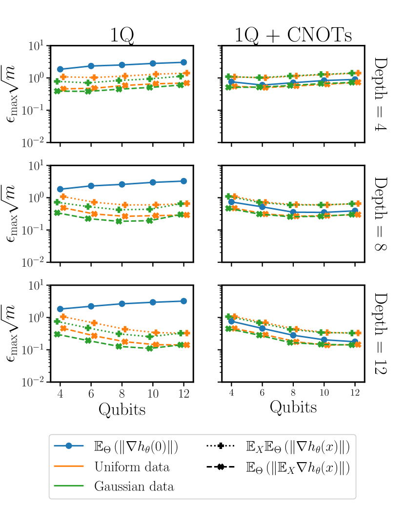
Figure 2: Results for $\epsilon_{\rm MAX}\sqrt{m}\approx\mathbb{E}_{X}\left(\mathbb{E}_{{\bm{\Theta}}}\left(\norm{\nabla h_{\bm{\theta}}(x)}\right)\right)$ (see Equation 44) for QRU models with alternating layered ansatzes. Data is introduced through controlled-rotation gates. Parameterized gates are single-qubit arbitrary operations. Each row has an increasing depth in the circuit. The right column includes CNOT gates for the base PQC. In the left column, gradients follow different trends for the cases with and without data, implying data can not be re-absorbed into a reparametrization, in the sense of Theorem III.1. In the right column, similar trends indicate large absorption capabilities.

In this section, we present our numerical results, focusing on the average gradient magnitudes of hypothesis functions generated by QRU models in comparison to base PQCs. This analysis serves to validate the findings presented in  Theorem III.1 regarding gradient variances and can be considered as a proxy for evaluating the absorption witnesses defined in  Definition III.1. We explore various ansatzes and use different data distributions for the experiments. Our code for these experiments is available in Barthe and Pérez-Salinas (2023), and the data can be provided upon request.

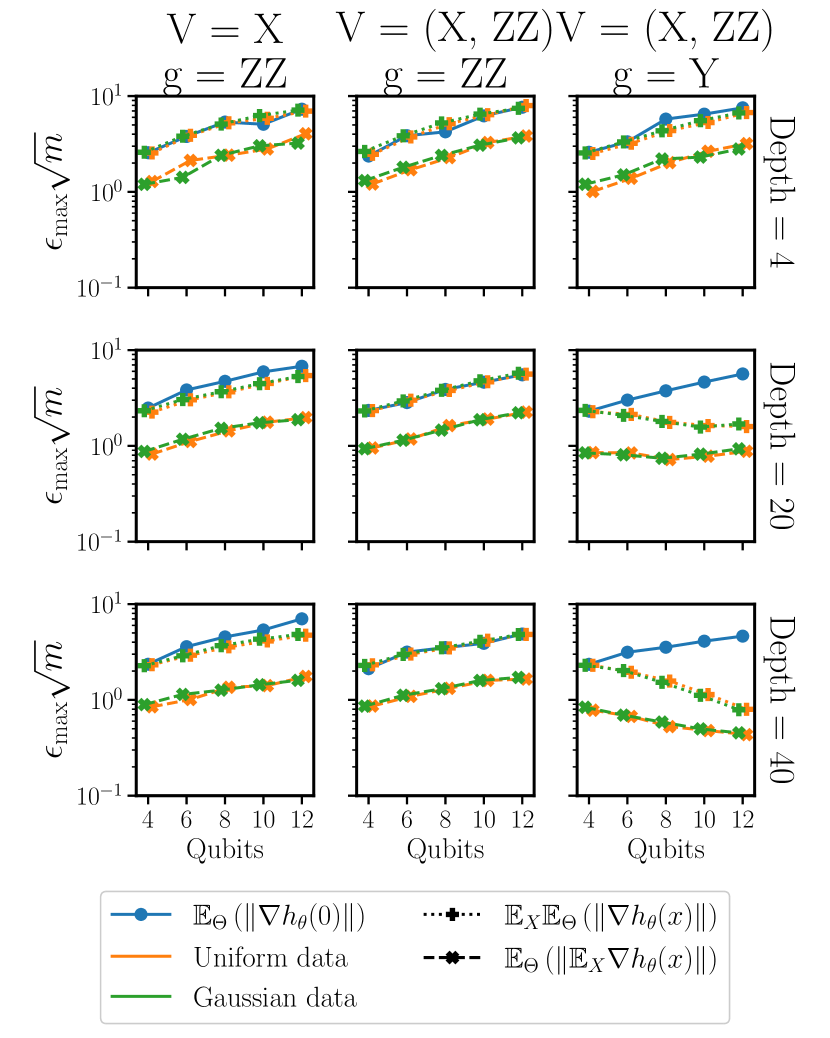
Figure 3: Results for $\epsilon_{\rm MAX}\sqrt{m}\approx\mathbb{E}_{X}\left(\mathbb{E}_{{\bm{\Theta}}}\left(\norm{\nabla h_{\bm{\theta}}(x)}\right)\right)$ (see Equation 44) for QRU models with translation-invariant layered ansatzes. Data is introduced through the generators $g$, and data through the generators $V$, indicated at the top for every column. Each row has an increasing depth in the circuit. In the left column, gradients follow approximately the same trends with and without data, implying high absorption capabilities in the sense of Theorem III.1. For the middle column, the absorption is total since it can be done by a simple shift of parameters. The right column reveals different trends for the cases with and without data, implying low absorption.

As a first example, we compare a re-uploading ansatz, consisting of single-qubit rotations and data-encoding entangling gates, with two different PQCs (see Figure 1). In both cases, we construct the hypothesis function measuring sums of single-qubit $X$ Pauli measurements. The addition of entangling gates in PQC2 with respect to PQC1 is essential to exploring entangled states, and it plays a role in addressing the issue of vanishing gradients Cerezo et al. (2021b). The data-encoding layer is a controlled operation $C-(XR_{z}(x))$, which can be absorbed into single-qubit and controlled rotations Barenco et al. (1995).

The results are shown in Figure 2. The columns correspond to the respective models (1-2), and the rows correspond to different depths of the ansatz. In the left column, corresponding to a PQC with only single-qubit gates, we observe a qualitative difference in the average gradients of the PQC and re-uploading circuits. The PQC is relatively insensitive to the number of qubits, as a consequence of the redundancy of multiple consecutive single-qubit gates. Adding data modifies this behavior. In the case of the entangling PQC (right column), the results without data align with previous works Cerezo et al. (2021b); Pérez-Salinas et al. (2023). The addition of data drawn from different distributions (Gaussian and uniform) introduces negligible differences in the results.

We turn our attention to translation-invariant ansatzes. These circuits are not capable of freely exploring the Hilbert space, but only its invariant subspace. This restriction reduces the freedom in these circuits, leading to an increase in the average gradients of the cost function for PQCs Larocca et al. (2021). We choose three layered models, based on the generators $X=\sum_{q}X_{q}$, $Y=\sum_{q}Y_{q}$, $ZZ=\sum_{q}Z_{q}Z_{q+1}$, where $q$ cyclically iterates over all qubits. In the first model, the generator associated with parameters is $V_{i}=X$, and data-encoding is conducted through $g=ZZ$. The second model is given by $\{V\}=\{X,ZZ\}$, $g=ZZ$. The third model is defined by $\{V\}=\{X,ZZ\}$, $g=Y$. In all cases, the observable considered is $X$. Among these models, only the second one can automatically absorb data into parameters through shifts. Gaussian-distributed data is used in all cases.

Results are detailed in Figure 3. The columns correspond to the respective models, and the rows correspond to different circuit depths. For each model, the average norm of the gradient scales differently with the number of qubits, with and without data. Models 1 and 2 present similar behavior when including data. In particular, for model 2 results show no difference between the re-uploading model and PQC since the data can be perfectly re-absorbed through a simple shift. A significant difference is noticeable in the third model. In this case, the absence of BPs in all instances makes the QRU models trainable by construction.

V.2 Expressivity

In  Section IV we prove a series of asymptotic results given some strong conditions related to the Haar randomness of the parametrized gates in between data uploading gates. In this section, we show the results of a series of numerical experiments in which such conditions are relaxed and show that the theoretical results still apply. We use three models to test different situations. The first two models are constructed with permutation-invariant generators, which correspond to PQC that have been proven to be trainable Schatzki et al. (2022). Those models express only the symmetric subspace in the available Hilbert space. In the first model (A), $g=X,V=ZZ$, and the second model (B) $g=X,V=\{Y,X,ZZ\}$. For the third model, $g=X$, and the parameterized pieces are sampled from the Haar measure, that is the set $V$ is free. We choose these models to have full control of the spectrum of the generator $\mathcal{K}_{g=X}$, which allows us to informatively compare to the theorems. All experiments were conducted with systems of $4$ qubits unless explicitly stated, without affecting the scaling of the obtained results.

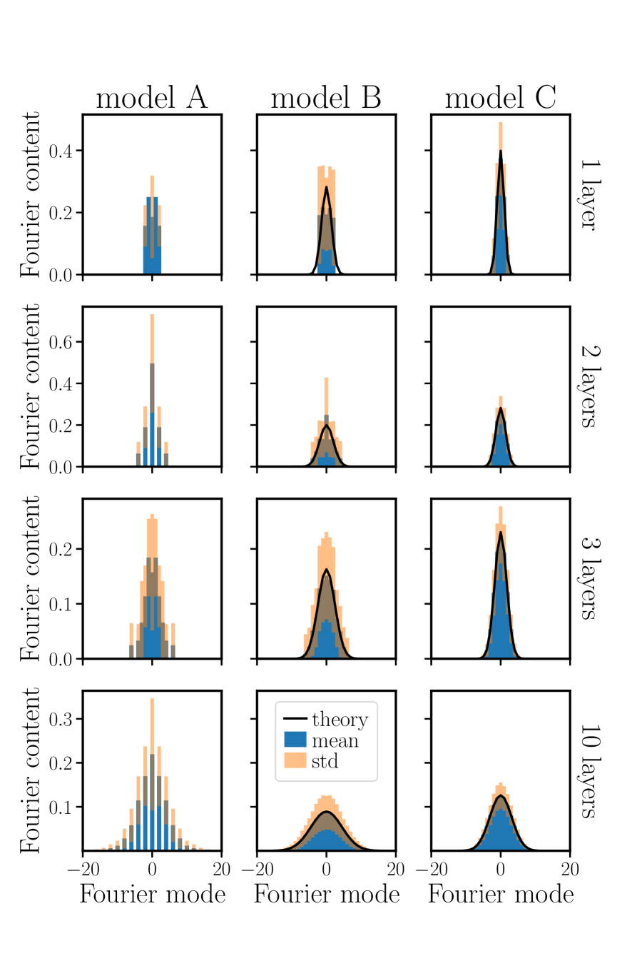
Figure 4: Evolution of frequency spectrum with the number of layers, for models (A, B, C) detailed in the first paragraph of the section. The Fourier content refers to (average and standard deviation of) $|c_{k}|^{2}$. Model (A) is not general enough to follow Theorem IV.1, but still, a spread in frequencies is observed. Model (B) is permutation-invariant and almost fully general in the symmetric space, and model (C) is general with no restrictions in the Hilbert space. As $L$ increases, the Fourier spectrum approximates a Gaussian profile with increasing variance according Equation 29. The values $\sigma_{g}$ for models (B) and (C) change due to the constraint in the available space.

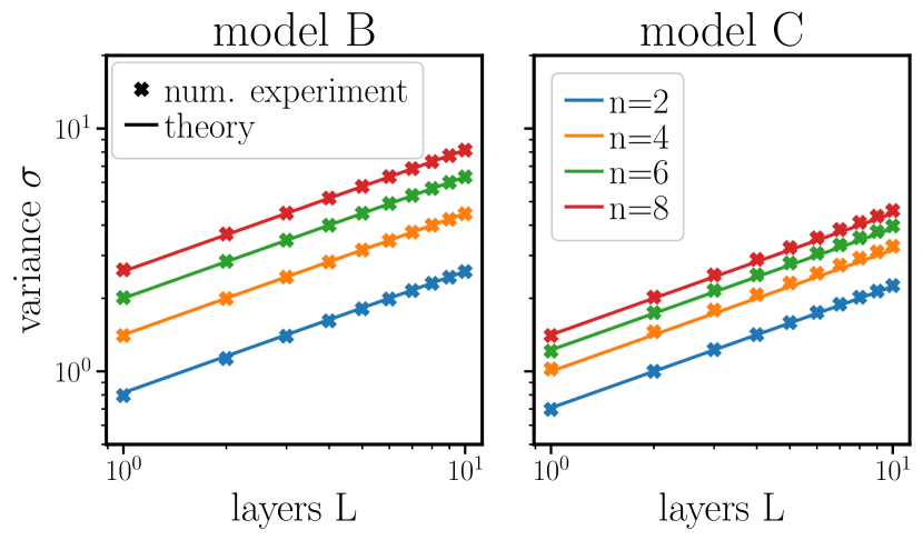
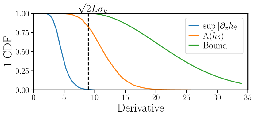
Figure 5: Variances for the tending-to-Gaussian profiles from Figure 4, for different numbers of qubits, in the y-axis, while the x-axis corresponds to the number of layers. The left figure corresponds to model (B), with $\sigma_{g}^{2}=n(n+2)/12$. The right figure corresponds to model (C), with $\sigma_{g}^{2}=n/4$. The scaling in $\sqrt{L}$ is in agreement with Equation 29.

Figure 6: Inverse CDFs for the optimal Lipschitz constants and $\Lambda(h_{\bm{\theta}})$, as compared to the bounds from Theorem IV.3. The x-axis indicate the value for each CDF, respectively $\sup_{x}|\partial_{x}h_{\bm{\theta}}(x)|$, $\Lambda(h_{\bm{\theta}})$ and $t$ for each line.

The first experiment tests Theorem IV.1 and Corollary IV.1, and the results can be seen in Figure 4. In model (A), the spectrum spreads towards large frequencies with the number of data re-uploadings. The parameterized gates are not general enough to support the theoretical results. For models (B) and (C), the Gaussian limit is matched even for a moderately small number of layers. This means that even though the theorem is proven for Haar random unitaries, the vanishing high-frequencies behavior still holds for model (B), even though the Haar condition is not guaranteed. Notice the difference in spreads for models (B) and (C). This is a consequence of the space explored by the ansatz. Model (B) is composed of a permutation invariant ansatz, and it is as general as possible only in the symmetric subspace, of dimension $n+1$. In this scenario, the spectrum of the corresponding $g$ is flat (see the results for 1 layer in figure 4), and the spread depends on the number of qubits $n$ as $\sigma_{g}=\mathcal{O}\left(n\right)$. For the model (C), the spectrum of $g$ with no restriction follows a binomial distribution, centered in $k=0$, with $\sigma_{g}\in\mathcal{O}\left(\sqrt{n}\right)$. A comparison between the theoretical and observed variances can be found in Figure 6, showing high agreement with the theoretical results.

We numerically check Theorem IV.3 in Figure 6. We depict in this figure the observed cumulative distribution functions (CDF) of both the numerically found LB, and $\Lambda(h_{\bm{\theta}})$ defined in Equation 32. These CDFs are compared to the upper bound from Theorem IV.3. Results show agreement with Theorem IV.3, and even indicate the possibility of finding tighter bounds, at least in terms of prefactors.

V.3 Training

All the LB results describe an average behavior for ${\bm{\Theta}}$. In this subsection, we briefly explore the effect of previous results in the training. We task model (B) to learn functions whose Fourier coefficients follow a step function of increasing width. This approximately corresponds to a cardinal sinus of decreasing width.

We display results of trained QRU models in Figure 7. In the top figure, we show the Fourier components of different functions to be fitted (in dashed lines), and the hypothesis functions after training (solid lines). The target function is learned by the model for $K\leq 20$ but the hypothesis function fails to capture high frequencies from $k>25$. Notice that the obtained hypothesis functions for $K=\{30,40\}$ seem to saturate the expressivity capabilities of the model. The bottom figure represents the functions in the data domain for $K=\{4,40\}$.

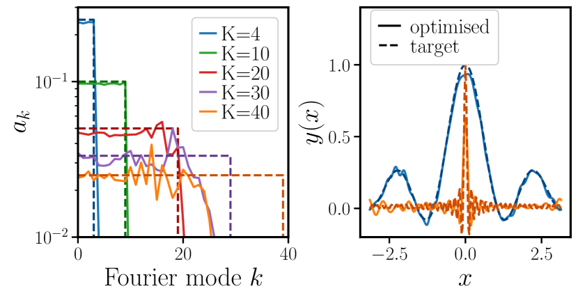
Figure 7: Results in both in time and frequency domains of circuits trained to match increasingly precise cardinal sinus, implying increasing high-frequency content. The circuit used is model (B). Starting from frequency 20 the model is not able to lift the amplitude.

VI Discussion

We turn our attention first to gradients. From our results, we can infer that vanishing gradients are avoided in QRU models if the base PQC is BP-free, and data can be absorbed into the parameterized gates. We can refer to existing literature on avoiding BPs for PQCs by restricting the dimensionality of the search space, by means of the dynamical Lie algebra Larocca et al. (2021); Schatzki et al. (2022). In a nutshell, the Lie algebra depends on the generators of the quantum model. Absorption witnesses can only be maintained close to $0$ if the base PQC and the derived QRU model share their Lie algebra. This observation allows one to choose data-encoding generators avoiding the emergence of BPs.

The average of $\Lambda(h_{\bm{\theta}})$ is a consequence of the vanishing high frequencies behavior that grows as $\sim\sigma_{g}\sqrt{L}$, as imposed by the central limit theorem. Deviating from this average is exponentially unlikely, as proven in theorem IV.3. As discussed later, it is in principle possible to amplify high-frequency components, at the expense of losing all degrees of freedom in the process. Therefore, for practical purposes, we need to adjust the number of re-uploading layers according to the scaling $\sim\sqrt{L}$, and not $\sim L$, as suggested by other theoretical works on expressivity via generalization bounds Caro et al. (2021).

In this work we derived the the scaling of the Fourier spectrum of hypothesis functions with the number of layers, but not with the number of qubits $n$. Our numerical simulations focus on frequency spaces increasing polynomially with $n$. However, it is possible to construct data-generators with exponentially many equally probable different accessible frequencies Shin et al. (2023). In this scenario, Theorem IV.1 still holds, leading to a Gaussian profile of frequencies with variance $\sigma\in\Theta(2^{n}\sqrt{L})$. Note that exponentially many frequencies require exponentially many tunable parameters to match the number of degrees of freedom. Therefore, data-encoding generators with $\sim e^{n}$ different frequencies can only aim to efficiently learn functions with sparse Fourier representations, i.e. with only $\mathcal{O}({\rm poly}(n))$ non-zero Fourier coefficients in a $\mathcal{O}(e^{n})$ frequency space.

The expressivity results from Section IV imply direct limitations in the attainable hypothesis functions, but also give an intuition on how to amplify high-frequency Fourier components, or in other words how to maximize the Lipschitz constant. The only recipe to obtain a high-frequency Fourier profile is by repeatedly amplifying the eigenvectors corresponding to extreme eigenvalues of the data-encoding generator. Without loss of generality, we may choose the ground state. The first step of the circuit would have to transform the initial state into the ground state of the data-encoding generator. For $k$-local Hamiltonians with $k\geq 2$, this problem is QMA-complete Kempe et al. (2005). An example is choosing the data generator to be the Hamiltonian of a transverse-field Ising model, constructed on an arbitrary graph. Such PQC does not suffer from BPs if the parameters respect the permutation invariance of the graph Larocca et al. (2021). Therefore, reaching the hypothesis function with maximized high-frequency content is in general hard. Finding the hypothesis function with maximum high-frequency content implies solving a QMA-complete problem several times. A notable exception appears in layered circuits with one $g$, and $W_{i}=I$, where setting all parameters $\theta=0$ suffices to maintain the quantum state aligned with the ground state of $g$. Notably, maximizing the Lipschitz constant in the experiments from Section V is feasible.

We have seen that hypothesis functions produced by layered QRU models have naturally vanishing high-frequency components, therefore limiting their Lipschitz constant. Regularization of the Lipschitz constant yields increased generalization and robustness of classical Neural Networks Gouk et al. (2021); Bartlett et al. (2017). As a consequence, this could hint toward a better generalization capacity of QRU models, in agreement with existing literature Peters and Schuld (2022).

VII Conclusions

We have explored the features of QRU models to understand the implications of injecting data into the better-studied PQCs models. Two main features are studied, first the magnitude of the gradients of the loss function, and second the frequency profile of the hypothesis function output by QRU models. Results were proven analytically and extended to more practical scenarios numerically.

We give analytical bounds for the connection between the variance of gradients in the hypothesis functions of QRU models and the cost functions on corresponding PQCs. Vanishing gradients of hypothesis functions imply vanishing gradients for any cost function to train ML models with, thus preventing trainability. The difference between QRU models and PQCs can be quantified by measuring the effect of adding data to the circuit, averaging over the parameter space. This is quantified by the coined concept of absorption witness. If data can be re-absorbed in a shift of parameters, then the gradients for PQCs and QRU models take similar value ranges. Results can be further simplified for the case of layered ansatzes. These results provide insights into the construction of QRU models protected against the phenomenon of BP, by using existing knowledge on PQC that do not exhibit BPs.

We prove also that QRU models suffer from vanishing high frequencies. Each additional data encoding operation corresponds to an additional convolution of the current spectrum with the data generator spectrum. As the number of layers, denoted as $L$, becomes large the span of attainable frequencies grows as $\mathcal{O}\left(L\right)$. However, the central limit theorem dictates that the frequency profile follows a Gaussian distribution, spreading out proportionally to $\sqrt{L}$. Therefore, in practice, only frequencies (approximately) bounded by $\sqrt{L}$ are available, with the contribution of higher frequencies exponentially vanishing. The vanishing high frequencies have direct consequences on the class of functions attainable by the QRU models. The average of the optimal Lipschitz constant scales with $\sqrt{L}$, exhibiting an exponentially decaying probability of exceeding this value. These findings offer insights into the inherent limitations of expressivity in QRU models and provide tools for estimating the computational resources required to represent specific datasets effectively.

The results derived in this work broaden our understanding of the properties of QRU models and provide guidelines for the design of re-uploading schemes. As an example, the concept of absorption witness can be employed to select generators ensuring an ansatz with the necessary characteristics to be trainable. For expressivity, adjusting the depth of the model can strike a balance between capturing intricate details in the data and avoiding overfitting. Consequently, we anticipate that these tools and insights will contribute to enhancing the applicability and performance of QRU models.

Appendix A Proofs

A.1 Proof of Theorem III.1

We begin by explicitly writing the derivatives of the hypothesis function

$$\partial_{j}h_{{\bm{\theta}}}(x)=\Tr{U_{R,j}({\bm{\theta}}_{R,j},x)\ \rho_{0}U^{\dagger}_{R,j}({\bm{\theta}}_{R,j},x)\left[V_{j},U^{\dagger}_{L,j}({\bm{\theta}}_{L,j},x)HU_{L,j}({\bm{\theta}}_{L,j},x)\right]}.$$ (45)

In this equation, the indices $R,L$ indicate all operations before and after the $j-$th operation. We redefine the quantities for readability

$$\rho_{j}({\bm{\theta}}_{R,j},x) =U_{R,j}({\bm{\theta}}_{R,j},x)\ \rho_{0}\ U^{\dagger}_{R,j}({\bm{\theta}}_{R,j},x)$$ (46)

$$H_{j}({\bm{\theta}}_{L,j},x) =U^{\dagger}_{L,j}({\bm{\theta}}_{L,j},x)\ H\ U_{L,j}({\bm{\theta}}_{L,j},x)$$ (47)

The variance of these derivatives over ${\bm{\Theta}}$ is given by

$$\mathbb{E}_{X}\left(\operatorname{Var}_{{\bm{\Theta}}}\left(\partial_{j}h_{{\bm{\theta}}}(x)\right)\right)=\mathbb{E}_{{\bm{\Theta}}}\left(\operatorname{Var}_{X}\left(\partial_{j}h_{{\bm{\theta}}}(x)\right)\right)=\mathbb{E}_{{\bm{\Theta}}_{R,j}}\left(\mathbb{E}_{{\bm{\Theta}}_{L,j}}\left(\mathbb{E}_{X}\left(\left(\partial_{j}h_{{\bm{\theta}}}(x)\right)^{2}\right)\right)\right),$$ (48)

where we assume no correlation between the parameters in the left and right parts of the circuit. By calling the property $\Tr{A\otimes B}=\Tr A\Tr B$, we can plug Equation 45 into Equation 48 to obtain

$$\operatorname{Var}_{{\bm{\Theta}},X}\left(\partial_{j}h_{{\bm{\theta}}}(x)\right)=\mathbb{E}_{{\bm{\Theta}}_{R,j}}\left(\mathbb{E}_{{\bm{\Theta}}_{L,j}}\left(\mathbb{E}_{X}\left(\Tr{\rho_{j}({\bm{\theta}}_{R,j},x)^{\otimes 2}\left[V_{j},H_{j}({\bm{\theta}}_{L,j},x)\right]^{\otimes 2}}\right)\right)\right)$$ (49)

We aim to describe this quantity in terms of the difference between the QML models, partially described by data $x$, and their corresponding PQC models, where $x=0$. We define the corresponding difference operators

$$B_{R,j}^{(t)}({\bm{\theta}}_{R,j},x;\rho_{0}) =\rho_{j}^{\otimes t}({\bm{\theta}}_{R,j},x)-\rho_{j}^{\otimes t}({\bm{\theta}}_{R,j},0)$$ (50)

$$B_{L,j}^{(t)}({\bm{\theta}}_{L,j},x;H) =H_{j}^{\otimes t}({\bm{\theta}}_{L,j},x)-H_{j}^{\otimes t}({\bm{\theta}}_{L,j},0).$$ (51)

We rearrange the terms in the integrand of Equation 49 as

$$\Tr{\rho_{j}({\bm{\theta}}_{R,j},x)^{\otimes 2}\left[V_{j},H_{j}({\bm{\theta}}_{L,j},x)\right]^{\otimes 2}} =$$ (52)

$$\Tr{\rho_{j}({\bm{\theta}}_{R,j},0)^{\otimes 2}[V_{j},H_{j}({\bm{\theta}}_{R,j},x)]^{\otimes 2}} +\Tr{B_{R,j}^{(2)}({\bm{\theta}}_{R,j},x;\rho_{0})[V_{j},H_{j}({\bm{\theta}}_{L,j},x)]^{\otimes 2}}=$$ (53)

$$\Tr{H_{j}({\bm{\theta}}_{R,j},x)^{\otimes 2}[\rho_{j}({\bm{\theta}}_{R,j},0),V_{j}]^{\otimes 2}} +\Tr{B_{R,j}^{(2)}({\bm{\theta}}_{R,j},x;\rho_{0})[V_{j},H_{j}({\bm{\theta}}_{L,j},x)]^{\otimes 2}}=$$ (54)

$$\Tr{\rho_{j}({\bm{\theta}}_{R,j},0)^{\otimes 2}[V_{j},H_{j}({\bm{\theta}}_{R,j},0)]^{\otimes 2}}+$$ (55)

$$\Tr{B_{R,j}^{(2)}({\bm{\theta}}_{R,j},x;\rho_{0})[V_{j},H_{j}({\bm{\theta}}_{L,j},x)]^{\otimes 2}}+$$ (56)

$$\Tr{B_{L,j}^{(2)}({\bm{\theta}}_{L,j},x;H)[\rho_{j}({\bm{\theta}}_{R,j},0),V_{j}]^{\otimes 2}}$$ (57)

by recalling the identities $\Tr{A^{\otimes 2}}=\Tr{A}^{2}$ and $\Tr{A[B,C]}=\Tr{B[C,A]}=\Tr{C[A,B]}$. The term in Equation 55 corresponds to the standard variance in PQC. We denote it simply as $\operatorname{Var}_{{\bm{\Theta}}}\left(\partial_{j}h_{\bm{\theta}}(0)\right).$

We move our attention now Equation 56. This term measures the difference between QRU models and PQC in the right part of the quantum circuit. Assuming that the right and left parameters are uncorrelated, we can rewrite

$$\mathbb{E}_{{\bm{\Theta}}_{R,j}}\left(\mathbb{E}_{{\bm{\Theta}}_{L,j}}\left(\mathbb{E}_{X}\left(\Tr{B_{R,j}^{(2)}({\bm{\theta}}_{R,j},x;\rho_{0})\left[V_{j},H({\bm{\theta}}_{L,j},x)\right]^{\otimes 2}}\right)\right)\right)=\\ \Tr{\left(\mathbb{E}_{X}\left(\mathbb{E}_{{\bm{\Theta}}_{R,j}}\left(B_{R,j}^{(2)}({\bm{\theta}}_{R,j},x;\rho_{0})\right)\right)\right)\left[V_{j},\mathbb{E}_{{\bm{\Theta}}_{L,j}}\left(H({\bm{\theta}}_{L,j},x)\right)\right]^{\otimes 2}}$$ (58)

Using Hölder inequality

$$|\Tr{AB}|\leq\norm{A}_{2}\norm{B}_{2},$$ (59)

in Equation 58 together with the triangular and Cauchy-Schwarz inequality we obtain

$$\left|\mathbb{E}_{X}\left(\Tr{\mathbb{E}_{{\bm{\Theta}}_{R,j}}\left(B_{R,j}^{(2)}({\bm{\theta}}_{R,j},x;\rho_{0})\right)}\left[V_{j},\mathbb{E}_{{\bm{\Theta}}_{L,j}}\left(H({\bm{\theta}}_{L,j},x)\right)\right]^{\otimes 2}\right)\right|\leq\\ \mathbb{E}_{X}\left(\left|\Tr{\mathbb{E}_{{\bm{\Theta}}_{R,j}}\left(B_{R,j}^{(2)}({\bm{\theta}}_{R,j},x;\rho_{0})\right)}\left[V_{j},\mathbb{E}_{{\bm{\Theta}}_{L,j}}\left(H({\bm{\theta}}_{L,j},x)\right)\right]^{\otimes 2}\right|\right)\leq\\ \mathbb{E}_{X}\left(\norm{\mathbb{E}_{{\bm{\Theta}}_{L,j}}\left(\left[V_{j},H({\bm{\theta}}_{L,j},x)\right]^{\otimes 2}\right)}_{2}\ \norm{\mathbb{E}_{{\bm{\Theta}}_{R,j}}\left(B_{R,j}({\bm{\theta}}_{R,j},x;\rho_{0})\right)}_{2}\right).$$ (60)

Substituting in the previous equation the property Holmes et al. (2022)

$$\norm{\left[V_{j},H({\bm{\theta}}_{L,j},x)\right]^{\otimes 2}}_{2}\leq 4\norm{V_{j}}_{2}^{2}\norm{H}_{2}^{2},$$ (61)

and defining

$$\mathcal{B}^{(2)}_{R,j}(\rho_{0})=\mathbb{E}_{X}\left(\norm{\mathbb{E}_{{\bm{\Theta}}_{R,j}}\left(B\right)^{(2)}_{R,j}({\bm{\theta}}_{R,j},x;\rho_{0})}_{2}\right),$$ (62)

we obtain

$$\mathbb{E}_{{\bm{\Theta}}_{R,j}}\left(\mathbb{E}_{{\bm{\Theta}}_{L,j}}\left(\mathbb{E}_{X}\left(\Tr{B_{R,j}^{(2)}({\bm{\theta}}_{R,j},x;\rho_{0})\left[V_{j},H({\bm{\theta}}_{L,j},x)\right]^{\otimes 2}}\right)\right)\right)\leq 4\norm{V_{j}}_{2}^{2}\norm{H}_{2}^{2}\ \mathcal{B}^{(2)}_{R,j}(\rho_{0}).$$ (63)

Following the same steps for Equation 57, we can bound this quantity as

$$\mathbb{E}_{{\bm{\Theta}}_{R,j}}\left(\mathbb{E}_{{\bm{\Theta}}_{L,j}}\left(\mathbb{E}_{X}\left(\Tr{B_{L,j}^{(2)}({\bm{\theta}}_{L,j},x;H)[V_{j},\rho_{R}({\bm{\theta}}_{R,j},0)]^{\otimes 2}}\right)\right)\right)\leq 4\norm{V_{j}}_{2}^{2}\norm{\rho_{0}}_{2}^{2}\ \mathcal{B}^{(2)}_{L,j}(H),$$ (64)

where we defined analogously

$$\mathcal{B}^{(2)}_{L,j}(H)=\mathbb{E}_{X}\left(\norm{\mathbb{E}_{{\bm{\Theta}}_{L,j}}\left(B^{(2)}_{L,j}({\bm{\theta}}_{L,j},x;H)\right)}_{2}\right).$$ (65)

Notice that we could interchange the $x$-dependency in Equation 57 and Equation 56 with no effect in the final bounds. The reason is that Equation 61 eliminates the $x$-dependency in the term where it is applied.

We can compact the results from Equations (63) and (64) using the triangular inequality in

$$\left|\operatorname{Var}_{{\bm{\Theta}}}\left(\partial_{j}h_{\bm{\theta}}(0)\right)-\operatorname{Var}_{{\bm{\Theta}}}\left(\mathbb{E}_{X}\left(\partial_{j}h_{{\bm{\theta}}}(x)\right)\right)\right|\leq 4\norm{V_{j}}_{2}^{2}\left(\norm{H}_{2}^{2}\ \mathcal{B}^{(2)}_{R,j}(\rho_{0})+\ \norm{\rho_{0}}_{2}^{2}\ \mathcal{B}^{(2)}_{L,j}(h)\right)$$ (66)

∎

A.2 Proof of Lemma III.1

We start by bounding the right absorption witness of the $(l+1)$-th layer with the triangular and Hölder’s inequality as

$$\mathcal{B}^{(2)}_{R,l+1}(\rho_{0})=\mathbb{E}_{X}\left(\norm{\mathbb{E}_{{\bm{\Theta}}_{l+1}}\left(u({\bm{\theta}}_{l+1})^{\otimes 2}V(x)^{\otimes 2}\ \mathbb{E}_{{\bm{\Theta}}_{R,l}}\left(\rho_{l}({\bm{\theta}}_{R,l},x)\right)V^{\dagger}(x)^{\otimes 2}u^{\dagger}({\bm{\theta}}_{l+1})^{\otimes 2}\right)}_{2}\right)\leq\\ \mathbb{E}_{X}\left(\norm{\mathbb{E}_{{\bm{\Theta}}_{l+1}}\left(u({\bm{\theta}}_{l+1})^{\otimes 2}V(x)^{\otimes 2}\ \mathbb{E}_{{\bm{\Theta}}_{R,l}}\left(B^{(2)}_{R,l}({\bm{\theta}}_{R,l},x;\rho_{0})\right)V^{\dagger}(x)^{\otimes 2}u^{\dagger}({\bm{\theta}}_{l+1})^{\otimes 2}\right)}_{2}\right)+\\ \mathbb{E}_{X}\left(\norm{\mathbb{E}_{{\bm{\Theta}}_{l+1}}\left(u({\bm{\theta}}_{l+1})^{\otimes 2}V(x)^{\otimes 2}-u({\bm{\theta}}_{l+1})^{\otimes 2}\right)}_{2}\norm{\mathbb{E}_{{\bm{\Theta}}_{R,l}}\left(\rho_{l}({\bm{\theta}}_{R,l},0)\right)}_{2}\right)$$ (67)

The second term can be identified as the layerwise absorption witness from Definition III.2. The first term of the equation above can be bounded as

$$\mathbb{E}_{X}\left(\norm{\mathbb{E}_{{\bm{\Theta}}_{l+1}}\left(u({\bm{\theta}}_{l+1})^{\otimes 2}V(x)^{\otimes 2}\ \mathbb{E}_{{\bm{\Theta}}_{R,l}}\left(B^{(2)}_{R,l}({\bm{\theta}}_{R,l},x;\rho_{0})\right)V^{\dagger}(x)^{\otimes 2}u^{\dagger}({\bm{\theta}}_{l+1})^{\otimes 2}\right)}_{2}\right)\leq\\ \mathbb{E}_{X}\left(\mathbb{E}_{{\bm{\Theta}}_{l+1}}\left(\norm{u({\bm{\theta}}_{l+1})^{\otimes 2}V(x)^{\otimes 2}\ \mathbb{E}_{{\bm{\Theta}}_{R,l}}\left(B^{(2)}_{R,l}({\bm{\theta}}_{R,l},x;\rho_{0})\right)V^{\dagger}(x)^{\otimes 2}u^{\dagger}({\bm{\theta}}_{l+1})^{\otimes 2}}_{2}\right)\right)=\mathcal{B}^{(2)}_{R,l}(\rho_{0}).$$ (68)

Arranging both results together we can find

$$\mathcal{B}^{(2)}_{R,l+1}(\rho_{0})\leq\mathcal{B}^{(2)}_{R,l}(\rho_{0})+\norm{\rho_{0}}_{2}^{2}\mathcal{A}_{l+1}^{(2)}.$$ (69)

Equivalently for the left part of the circuit, and counting layers backward we find

$$\mathcal{B}^{(2)}_{L,l}(H)\leq\mathcal{B}^{(2)}_{L,l+1}(\rho_{0})+\norm{H}_{2}^{2}\mathcal{A}_{l}^{(2)}.$$ (70)

∎

A.3 Details on harmonic representation of QRU models

As stated in Equation 24, the wavefunction after a re-uploading circuit and before measurement can be expressed as

$$\ket{\psi(x)}=\sum_{j=1}^{2^{n}}\sum_{k=-K}^{K}c_{k,j}e^{ikx}\ket{j}.$$ (71)

The coefficients $c_{k,j}$ form the matrix $\bm{C}\in\mathbb{C}^{2^{n}\times(2K+1)}$. Each column (indexed with $k$) represents the corresponding term $e^{ikx}$. The states $\ket{j}$ are elements of any basis of choice. Each row (indexed with $j$) corresponds to the $x$-dependent amplitude attached $\ket{j}$. The quantity $p_{j}(x)=\innerproduct{j}{\psi(x)}$ is a trigonometric polynomial, $p_{j}(x)=\sum_{k=-K}^{K}c_{k,j}e^{ikx}$. Such polynomial can be represented as a vector $p_{j}=\left\{c_{k,j}\right\}_{-K\leq k\leq+K}$. In this vector representation, the multiplication of polynomials corresponds to convolution as

$$p(x)q(x)=\sum_{k=-K_{p}}^{K_{p}}p_{k}e^{ikx}\sum_{k=-K_{q}}^{K_{q}}q_{k}e^{ikx}=(p*q)(x),$$ (72)

We consider the three operations that can be applied to the harmonic representation.

Parametrized gates

Applying a parameterized gate on the quantum state maps into applying the unitary representation of that gate to each column individually, the same way it would be done in state vector simulation for each (fixed) $k$.

Data-encoding gates

Adding a data-encoding gate involves convolution, when $\bm{C}$ is expressed in the eigenbasis of the data generator. Each row $j$ corresponds to the $j$-th (integer) eigenvalue $\lambda_{j}$ from the spectrum of the data-encoding generator, $\mathcal{K}_{g}$. The vector representation of polynomials $p_{j}$ is convoluted with the vector $e_{\lambda_{j}}=[\delta_{k=\lambda_{j}}]_{-K\leq k\leq+K}$.

Measurement

For the measurement, we express $\bm{C}$ the basis of the observable. Secondly the representation the transpose conjugate of the wavefunction is computed from $\bm{C}$, by taking its conjugate and reverting the rows indexing $c_{j,k}=c_{j,-k}$. Finally the hypothesis function $h_{{\bm{\theta}}}(x)$ can be obtained as a linear combination of the rows of the result of the convolution weighted by the corresponding eigenvalue of the measurement operator.

A.4 Proof of Theorem IV.1

We assume now that the parameterized gates between two consecutive encoding steps are random unitaries sampled from the Haar measure of the group $\mathcal{SU}(N)$. Notice that data-independent operations leave the norm of coefficients associated with the same frequency invariant. Random unitaries output random states for any input. Random states give rise to a probability distribution sampled from a uniform Dirichlet Dirichlet (2008), also known as Porter-Thomas Boixo et al. (2018) distribution. Under this assumption, no basis has any preference over any other, and the application of the data encoding layer transports as many coefficients as dictated by the spectrum $\mathcal{K}_{g_{j}}$ to the corresponding new frequencies. Notice that it is irrelevant which coefficients are transported, and also they are randomly chosen. The weights for the elements of each frequency are then described by a Dirichlet distribution with parameters given by the convoluted spectrum. Formally,

$$\sum_{j}\left|c_{k,j}\right|^{2}\sim\operatorname{Dir}\left(\left(\mathcal{K}_{g_{1}}\ast\ldots\ast\mathcal{K}_{g_{j}}\ast\ldots\ast\mathcal{K}_{g_{L}}\right)(k)\right),$$ (73)

where $*$ denotes the convolution operator. Notice that the index $k$ runs over all non-zero entries of the convoluted spectra. ∎

A.5 Proof of Corollary IV.2

Let us express the wavefunction as the $\bm{C}$ matrix, such that the wavefunction is reconstructed from its elements as

$$\ket{\psi(x)}=\sum_{j=1}^{2^{n}}\sum_{k=-K}^{K}c_{k,j}e^{ik\mu x}\ket{j},$$ (74)

where $\ket{j}$ is expressed in this case the eigenbasis of the observable of interest $H$. We are interested in the function

$$h(x)=\bra{\psi(x)}H\ket{\psi(x)},$$ (75)

which in the eigenbasis of $H$ is

$$h(x)=\sum_{j}\sum_{k}\sum_{l}\lambda_{j}c_{k,j}c^{*}_{l,j}e^{i\mu(k-l)\ x}.$$ (76)

We give a bound now on the terms sharing the same frequencies

$$\left|\sum_{j}\sum_{k-l=\omega}\lambda_{j}c_{k,j}c^{*}_{l,j}\right|^{2}\leq\norm{H}_{\lambda}^{2}\left|\sum_{j}\sum_{k-l=\omega}c_{k,j}c^{*}_{l,j}\right|^{2}\leq\norm{H}_{\lambda}^{2}\sum_{k-l=\omega}\left(\sum_{j}\left|c_{k,j}\right|^{2}\right)\left(\sum_{j}\left|c_{l,j}\right|^{2}\right),$$ (77)

where we used the triangular inequality and the Cauchy-Schwarz inequality. The last term is related to Theorem IV.1. Each of these elements is drawn from the Dirichlet distribution imposed by the spectrum $\mathcal{K}_{g}^{*L}$. The aggregation property of Dirichlet distributions allows us to directly work with the spectrums. The spectrum of interest is a modified convolution of $\mathcal{K}_{g}^{*L}$ with itself under an inversion of the variable, namely

$$\sum_{k-l=\omega}\mathcal{K}_{g}^{*L}(k)\mathcal{K}_{g}^{*L}(l)=\sum_{k}\mathcal{K}_{g}^{*L}(k)\mathcal{K}_{g}^{*L}(k-\omega)=\sum_{k}\mathcal{K}_{g}^{*L}(k)\mathcal{K}_{g}^{*L}(-(k-\omega))=\left(\mathcal{K}_{g}^{*L}*\mathcal{K}_{g}^{\prime\ *L}\right)(\omega),$$ (78)

with $\mathcal{K}_{g}^{*L}(x)=\mathcal{K}_{g}^{\prime\ *L}(-x)$. In the case of symmetric spectra, both functions are equivalent. Recalling the properties of Dirichlet distributions, we can bound

$$\norm{H}_{\lambda}^{-2}\left|a_{\omega}({\bm{\theta}})\right|^{2}\leq p_{\omega}\sim\operatorname{Dir}(\mathcal{K}_{g}^{*2L}(\omega)),$$ (79)

with

$$a_{\omega}({\bm{\theta}})=\sum_{j}\sum_{k-l=\omega}\lambda_{j}c_{k,j}c^{*}_{l,j}$$ (80)

∎

A.6 Proof of Theorem IV.2

We use tools from statistics to compute upper and lower bounds to the Lipschitz constant of a hypothesis function $\Lambda(h_{\bm{\theta}})$. We first recall the definition

$$\Lambda(h_{\bm{\theta}}):=\sum_{k=-K}^{K}\mu|k||a_{k}|,$$ (81)

and we recall the result from Corollary IV.2 in the limit of many re-uploadings. We know that

$$\mathbb{E}_{{\bm{\Theta}}}\left(\Lambda(h_{\bm{\theta}})\right)=\sum_{k=-K}^{K}\mu|k|\mathbb{E}_{{\bm{\Theta}}}\left(|a_{k}|\right).$$ (82)

We can use the known bound for the probability distribution underlying $|a_{k}|$, $|a_{k}|^{2}\leq p_{k}\sim\operatorname{Dir}(\mathcal{K}_{g}^{*L})$. In particular, the marginals of the Dirichlet distribution are beta distributions Bailey (1992). The beta probability distribution with parameters $\alpha$ and $\beta$ is defined as

$$\operatorname{Beta}_{\alpha,\beta}(x)=\frac{\Gamma(\alpha+\beta)}{\Gamma(\alpha)\Gamma(\beta)}x^{(\alpha-1)}(1-x)^{(\beta-1)}.$$ (83)

In our case, see Equation 31, $\alpha$ is given by the Gaussian spectrum and $\beta=1$. The expectation value of each element is given by

$$\mathbb{E}_{{\bm{\Theta}}}\left(|a_{k}|\right)\leq\int_{0}^{1}dx\frac{\Gamma(\alpha_{k}+1)}{\Gamma(\alpha_{k})}x^{(\alpha_{k}-1/2)}=\frac{\alpha_{k}}{\alpha_{k}+1/2}\leq 2\alpha_{k},$$ (84)

using the property of the gamma function $\Gamma(1+x)=x\Gamma(x)$. The last inequality allows us to compute an upper bound in the limit of many re-uploadings by just computing

$$\sum_{k=-K}^{K}\mu k\mathbb{E}_{{\bm{\Theta}}}\left(|a_{k}|\right)\leq 2\norm{H}_{\lambda}\sum_{k=-K}^{K}\mu k\mathcal{K}_{g}^{*2L}(k)\approx 4\norm{H}_{\lambda}\int_{0}^{\infty}\frac{\mu k}{\sqrt{4\pi L}\sigma_{g}}\exp\left(-\frac{k^{2}}{4\sigma^{2}_{g}L}\right)=\norm{H}_{\lambda}\frac{4}{\sqrt{\pi}}\sigma_{g}\mu\sqrt{L},$$ (85)

leading to the first result of the theorem.

The lower bound is easy to obtain by recalling the property $\norm{a}_{1}\geq\norm{a}_{2}$. In our context, and in the limit of Gaussian processes

$$\mathbb{E}_{{\bm{\Theta}}}\left(\Lambda(h_{\bm{\theta}})\right)^{2}\geq\norm{H}_{\lambda}^{2}\sum_{k=-K}^{K}\mu^{2}k^{2}\mathbb{E}_{{\bm{\Theta}}}\left(|a_{k}|^{2}\right)\approx\norm{H}_{\lambda}^{2}2L\mu^{2}\sigma_{g}^{2},$$ (86)

leading to the second result of the theorem: $\mathbb{E}_{{\bm{\Theta}}}\left(\Lambda(h_{\bm{\theta}})\right)\geq\norm{H}_{\lambda}\sigma_{g}\mu\sqrt{2L}$.∎

A.7 Proof of Theorem IV.3

We are interested in knowing the probability of $\Lambda(h_{\bm{\theta}})$ to be larger than a certain reference value by some distance. We take this reference value to be the average $\mathbb{E}_{{\bm{\Theta}}}\left(\Lambda(h_{\bm{\theta}})\right)$, as in many statistics results. Consider now the lower-bound on the expectation value from Theorem IV.2. Since

$$\Lambda(h_{\bm{\theta}})-\mathbb{E}_{{\bm{\Theta}}}\left(\Lambda(h_{\bm{\theta}})\right)\geq t\implies\Lambda(h_{\bm{\theta}})-\norm{H}_{\lambda}\mu\sqrt{2L}\sigma_{g}\geq t,$$ (87)

but not in the opposite direction, then

$$\operatorname{Prob}_{\bm{\Theta}}\left(\Lambda(h_{\bm{\theta}})-\mathbb{E}_{{\bm{\Theta}}}\left(\Lambda(h_{\bm{\theta}})\right)\geq t\right)\leq\operatorname{Prob}_{\bm{\Theta}}\left(\Lambda(h_{\bm{\theta}})-\norm{H}_{\lambda}\mu\sqrt{2L}\sigma_{g}\geq t\right).$$ (88)

We can bound the right hand by considering Hoeffding’s inequality Hoeffding (1963). Let ${X_{i}}$ be a set of independent random variables, and let $X_{i}\in[a_{i},b_{i}]$ almost surely, then

$$\operatorname{Prob}\left(\sum_{i}X_{i}-\mathbb{E}\left(\sum_{i}X_{i}\right)\geq t\right)\leq\frac{1}{2}\exp\left(\frac{-t^{2}}{\sum_{i}(a_{i}-b_{i})^{2}}\right).$$ (89)

Hoeffding’s inequality cannot be directly applied to a Dirichlet distribution since the variables are not independent. However, this problem can be overcome for this particular case by recalling the following property. If ${X_{i}}\sim\operatorname{Dir}(\alpha_{i})$, then

$$X_{i}\sim\frac{Y_{i}}{V},$$ (90)

with

$$Y_{i} \sim\operatorname{Gamma}(\alpha_{i},\theta)$$ (91)

$$V=\sum_{i}Y_{i} \sim\operatorname{Gamma}\left(\sum_{i}\alpha_{i},\theta\right)$$ (92)

By changing the description of the Dirichlet distribution to the quotient of gamma distributions we can now apply Hoeffding’s inequality. Without loss of generality, we can assume that all probabilities are bounded between $0$ and $1$, thus we can find a first bound by recalling

$$\sum_{n}n^{2}\in\mathcal{O}((\norm{g}_{\lambda}L)^{3}),$$ (93)

and thus

$$\operatorname{Prob}_{\bm{\Theta}}\left(\Lambda(h_{\bm{\theta}})-\mathbb{E}_{{\bm{\Theta}}}\left(\Lambda(h_{\bm{\theta}})\right)\geq t\right)\leq\operatorname{Prob}_{\bm{\Theta}}\left(\Lambda(h_{\bm{\theta}})-\norm{H}_{\lambda}\sqrt{2L}\mu\sigma_{g}\geq t\right)\in\mathcal{O}\left(\exp\left(\frac{-t^{2}}{(\norm{g}_{\lambda}L)^{3}}\right)\right)$$ (94)

∎

A.7.1 A tighter numerical bound

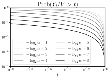
(a)  Numerical calculations for Equation 96 for decreasing values of $\alpha$. The values of the random variable concentrate in small values for $t$ as $\alpha$ decays.

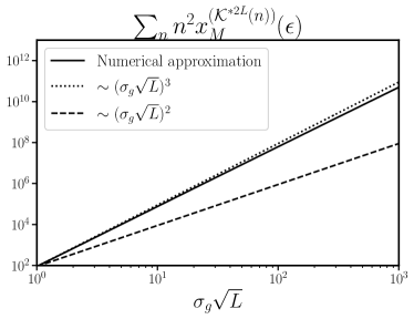
(b)  Numerical approximation to Equation 98 for increasing $\sigma_{g}\sqrt{L}$. The value $\epsilon$ is set in this calculations to $10^{-10}$

Figure 8: Numerical auxiliary calculations for Equation 96 and Equation 98. These results substitute the non-accessible analytical treatment of the probability distributions of interest to obtain the bound given in Equation 37

This bound can be however easily improved by recalling subgaussianity properties of the Gamma distribution. A random variable $X$ is subgaussian if its cumulative distribution function decays faster than exponentially

$$\operatorname{Prob}\left(|X|\geq t\right)\in\mathcal{O}\left(\exp\left(-t^{2}\right)\right),$$ (95)

for some positive constant $K$. We can compute this cumulative probability for the quotient of Gamma distributions as

$$\operatorname{Prob}\left(\frac{Y_{i}}{V}\geq t\right)=\int_{0}^{\infty}dx\int_{x}^{x/t}dy\frac{x^{\alpha-1}e^{-x}e^{-y}}{\Gamma(\alpha)}=\frac{1}{2^{\alpha}}-\frac{1}{(1+t^{-1})^{\alpha}}\in\mathcal{O}\left(\exp\left(-t^{2}\right)\right).$$ (96)

These functions take the value $1$ for $t=0$ and decay until vanishing for $t=1$. The decay is faster as $\alpha\rightarrow 0$, as it can be seen in Figure 8(a). We can thus recover Hoeffding’s inequality with the observation that each $X_{i}$ is bounded by the function in Equation 96. In particular, the variable $X_{i}$ is, with probability $1-\epsilon$, smaller than

$$x^{(\alpha_{i})}_{M}(\epsilon)=\left(\left(\frac{1}{2^{\alpha_{i}}}-\epsilon\right)^{-1/\alpha_{i}}-1\right)^{-1}.$$ (97)

For a sufficiently small $\epsilon$, the denominator of the exponent of Hoeffding’s inequality becomes

$$\sum_{n}(a_{n}-b_{n})^{2}=2\sum_{n=1}^{\norm{g}_{2}L}n^{2}x^{(\mathcal{K}_{g}^{*2L}(n))}_{M}(\epsilon),$$ (98)

with $\mathcal{K}_{g}^{*2L}$ a Gaussian spectrum in the limit of large $R$. The Gaussian limit forces the intuition that only a small number of elements will contribute effectively, while for large values of $n$ the corresponding Dirichlet variable is always so small that it has negligible influence in the Lipschitz constant. The description of the variable bounds in Equation 97 and the sum in Equation 98 prevent a straightforward analysis in terms of the relevant quantity $\sigma_{g}\sqrt{R}$. We can however make a numerical analysis, depicted in Figure 8(b). This calculation shows that the sum in Equation 98 follows a polynomial trend in $\sigma_{g}\sqrt{R}$, which is the variance of the resulting Gaussian spectrum. Therefore, we can update our previous version of Hoeffding’s inequality to

$$\operatorname{Prob}_{\bm{\Theta}}\left(\Lambda(h_{\bm{\theta}})-\norm{H}_{\lambda}\sqrt{2L}\sigma_{g}\geq t\right)\in\mathcal{O}\left(\exp\left(\frac{-t^{2}}{(\sigma_{g}\sqrt{L})^{3}}\right)\right).$$ (99)

A.8 Extension to non-harmonic spectrum

The non-harmonic extension leads to an average of the elements in the trigonometric polynomial given by

$$\mathbb{E}_{{\bm{\Theta}}}\left(|a_{\vec{k}}|^{2}\right)=\frac{1}{\sqrt{(4\pi L)^{D}|\Sigma|}}\exp\left(-\frac{\vec{k}^{T}\Sigma^{-1}\vec{k}}{4L}\right),$$ (100)

where $|\Sigma|$ is the determinant of $\Sigma$. We compute now $\Lambda(h_{\bm{\theta}})$ following the steps from Section A.6, given by

$$\mathbb{E}_{{\bm{\Theta}}}\left(\Lambda(h_{\bm{\theta}})\right)=\sum_{\vec{k}}|\vec{\mu}\cdot\vec{k}|\mathbb{E}_{{\bm{\Theta}}}\left(|a_{\vec{k}}|\right)\leq\frac{2}{\sqrt{(4\pi L)^{D}|\Sigma|}}\int_{\mathbb{R}^{D}}{d\vec{k}}|\vec{\mu}\cdot\vec{k}|\exp\left(-\frac{\vec{k}^{T}\Sigma^{-1}\vec{k}}{4L}\right).$$ (101)

Notice that $d\vec{k}$ integrates over $D$-dimensional space. We perform now a change the variables to diagonalize $\Sigma=U^{\dagger}SU$, and consequently choose $\vec{l}=U\vec{k}$. The diagonal elements of $S$ are denoted $\{s_{j}^{2}\}_{j}$ The quantity of interest is now $\vec{\mu}\cdot(U^{\dagger}\vec{l})=(U\vec{\mu})\cdot\vec{l}$. Since $U$ is unitary ${d\vec{l}}={d\vec{k}}$

$$\mathbb{E}_{{\bm{\Theta}}}\left(\Lambda(h_{\bm{\theta}})\right) \leq\frac{2}{\sqrt{(4\pi L)^{D}|\Sigma|}}\int_{\mathbb{R}^{D}}d\vec{l}|(U\vec{\mu})\cdot\vec{l}|\exp\left(-\frac{\vec{l}^{T}S^{-1}\vec{l}}{4L}\right)\leq$$ (102)

$$\frac{2}{\sqrt{(4\pi L)^{D}|\Sigma|}}\sum_{j=1}^{D}|(U\vec{\mu})_{j}|\int_{\mathbb{R}^{D}}d\vec{l}|l_{j}|\exp\left(-\frac{\vec{l}^{T}S^{-1}\vec{l}}{4L}\right)$$ (103)

We focus now on the integral.

$$\int_{\mathbb{R}^{D}}d\vec{l}|l_{j}|\exp\left(-\frac{\vec{l}^{T}S^{-1}\vec{l}}{4L}\right)= \int_{\mathbb{R}}dl_{j}|l_{j}|\exp\left(-\frac{\vec{l}_{j}^{2}}{4Ls_{j}^{2}}\right)\prod_{i\neq j}\int_{\mathbb{R}}dl_{i}\exp\left(-\frac{\vec{l}_{i}^{2}}{4Ls_{i}^{2}}\right)$$ (104)

$$=4Ls_{j}^{2}\prod_{i\neq j}\sqrt{4\pi Ls_{i}^{2}}=\frac{1}{\pi}\sqrt{(4\pi L)^{D+1}}\sqrt{|\Sigma|}s_{j}$$ (105)

Plugging this result into Equation 103 we obtain

$$\mathbb{E}_{{\bm{\Theta}}}\left(\Lambda(h_{\bm{\theta}})\right)\leq\frac{(2\sqrt{L\pi})^{D+1}}{\pi}\frac{\sqrt{|\Sigma|}|\vec{\mu}U^{\dagger}|\cdot\sqrt{\vec{S}}}{\sqrt{(4\pi L)^{D}|\Sigma|}}=\frac{4\sqrt{L}}{\sqrt{\pi}}\sum_{j=1}^{D}|U\vec{\mu}|_{j}s_{j}$$ (106)

By means of Cauchy-Schwarz inequality, we can give a looser yet more comprehensive bound as

$$\mathbb{E}_{{\bm{\Theta}}}\left(\Lambda(h_{\bm{\theta}})\right)\leq\frac{4}{\sqrt{\pi}}\norm{\vec{\mu}}_{2}\sqrt{\Tr(\Sigma)}\sqrt{L}.$$ (107)

For the lower bound we follow Section A.6 to obtain

$$\mathbb{E}_{{\bm{\Theta}}}\left(\Lambda(h_{\bm{\theta}})\right)^{2}\geq\norm{H}_{\lambda}^{2}\sum_{k=-K}^{K}(\vec{\mu}\cdot\vec{k})^{2}\mathbb{E}_{{\bm{\Theta}}}\left(|a_{k}|^{2}\right).$$ (108)

We recall the property Zee (2010); user26872 (2012)

$$\int d^{D}\vec{k}f(\vec{k})\exp\left(-\frac{\vec{k}^{T}\Sigma^{-1}k}{2}\right)=\sqrt{(2\pi)^{D}|\Sigma|}\left.\exp\left(\frac{\vec{\nabla}^{T}\Sigma^{-1}\vec{\nabla}}{2}\right)f(\vec{k})\right|_{\vec{k}=0},$$ (109)

where $\vec{\nabla}_{j}=\partial/\partial\vec{k}_{j}$. Since $f(\vec{k})=(\vec{\mu}\cdot\vec{k})^{2}$, we can reduce

$$\left.\exp\left(\frac{\vec{\nabla}^{T}\Sigma^{-1}\vec{\nabla}}{2}\right)f(\vec{k})\right|_{\vec{k}=0}=\vec{\mu}^{T}\Sigma\vec{\mu}\geq\norm{\vec{\mu}}_{2}^{2}{\rm min}_{\Lambda}(\Sigma),$$ (110)

yielding a result

$$\Lambda^{2}(h_{\bm{\theta}})\geq\norm{H}_{\lambda}^{2}2L\norm{\mu}_{2}^{2}{\rm min}_{\lambda}(\Sigma).$$ (111)

∎

A.8.1 A simple example

We illustrate the spectral convolution with an example. Consider a data generator whose spectrum and multiplicities are

$$\lambda =\{-\sqrt{2}-1,-\sqrt{2},-1,0,+1,+\sqrt{2},+\sqrt{2}+1\}$$ (112)

$$m(\lambda) =\{1,1,1,2,1,1,1\}$$ (113)

Any frequency resulting from the $L$-fold application of such data generator can be written as $\lambda_{k,l}=k\sqrt{2}+l$ where $-L\leq k,l\leq L$ are integers. The corresponding frequency content can therefore be represented as a two-dimensional tensor $A$. The elements of $A$ follow a 2-dimensional Dirichlet distribution, in the sense of Theorem IV.1, given by the convoluted kernel

$$\mathcal{K}_{g}^{*L}=\frac{1}{8}\begin{bmatrix}1&1&0\\ 1&2&1\\ 0&1&1\end{bmatrix}^{*L}$$ (114)

In the limit of large $L$, the central limit theorem applies exactly in the same way as in the harmonic case, and the $L$-fold convolution tends towards a multivariate Gaussian kernel with $[0,0]$ mean and covariance matrix

$$\Sigma=\frac{L}{2}\begin{pmatrix}1&0.5\\ 0.5&1\end{pmatrix}.$$ (115)