Adaptive Modelling Approach for Row-Type Dependent Predictive Analysis (RTDPA): A Framework for Designing Machine Learning Models for Credit Risk Analysis in Banking Sector

Abstract

In many real-world datasets, rows may have distinct characteristics and require different modeling approaches for accurate predictions. In this paper, we propose an adaptive modeling approach for row-type dependent predictive analysis(RTDPA). Our framework enables the development of models that can effectively handle diverse row types within a single dataset. Our dataset from XXX bank contains two different risk categories, personal loan and agriculture loan. each of them are categorised into four classes standard, sub-standard, doubtful and loss. We performed tailored data pre processing and feature engineering to different row types. We selected traditional machine learning predictive models and advanced ensemble techniques. Our findings indicate that all predictive approaches consistently achieve a precision rate of no less than $90\%$. For RTDPA, the algorithms are applied separately for each row type, allowing the models to capture the specific patterns and characteristics of each row type. This approach enables targeted predictions based on the row type, providing a more accurate and tailored classification for the given dataset.Additionally, the suggested model consistently offers decision makers valuable and enduring insights that are strategic in nature in banking sector.

Machine Learning, Credit Risk Analysis, agriculture loan prediction, personal loan prediction

1 Introduction

In many real-world datasets, the rows often exhibit distinct characteristics and necessitate different modeling approaches to achieve accurate predictions.For instance, when considering personal loans, agriculture loan,housing loans, and car loans, each category possesses unique attributes. Datasets frequently include rows encompassing multiple loan types, where certain attributes are specific to each loan type. For instance, a dataset may contain information about loans related to agriculture land, which can be further classified into dry land and wet land. However, these specific attributes related to land type may not be applicable to other loan types present in the dataset. In such cases, it becomes important to handle the varying attributes and loan types appropriately to ensure accurate analysis and modeling. Traditional modeling techniques tend to treat all rows in a dataset uniformly.[1][2]. However, this approach may overlook valuable information and hinder predictive performance.To address this challenge, we propose an adaptive modeling approach for row-type dependent predictive analysis. This approach recognizes and leverages the inherent heterogeneity of row types within a dataset, allowing for tailored modeling techniques to be applied to different row types. By adapting the modeling strategy to the unique characteristics of each row type, our approach aims to improve the accuracy and effectiveness of predictive models.

The key idea behind our adaptive modeling approach is to recognize that rows in a dataset may belong to distinct categories or types, each requiring specific modeling techniques. We start by separating the dataset based on row types, identifying the distinct categories present. For each row type, we then apply tailored data preprocessing techniques, such as handling missing values, addressing outliers, and performing feature engineering, to ensure that the data is appropriately prepared for modeling. This row-type-specific data preprocessing allows us to capture the unique characteristics and patterns associated with each row type more accurately.

Next, we select suitable predictive models for each row type based on its specific requirements and characteristics. These models include traditional statistical learning algorithms, such as logistic regression and machine learning algorithms such as decision trees, support vector machines, neural networks, K-nearest neighbour, as well as more advanced techniques, including ensemble methods or deep learning architectures. By choosing models specifically suited to the characteristics of each row type, we can better capture the underlying patterns and relationships within the data.

To train the models, we utilize the preprocessed data specific to each row type. This allows us to account for the distinct characteristics and potential variations in data distribution among different row types. Each model is trained using the corresponding subset of the dataset, ensuring that it captures the specific patterns and relationships relevant to that row type.

During the prediction phase, when encountering a new row, we identify its row type and select the corresponding model for making predictions. By adapting the model selection based on the row type, we ensure that the most appropriate model is used for accurate predictions. This adaptive selection mechanism allows us to effectively leverage the strengths of different models and achieve superior predictive performance.

2 Literature Review

Predictive modeling in the field of credit analysis has increasingly focused on analyzing datasets that encompass multiple credit categories[3][4]. Altman,et al. in his seminal paper introduced the concept of using financial ratios and discriminant analysis to predict corporate bankruptcy, laying the foundation for subsequent ML approaches in credit risk analysis. Smith et all.[5] conducted a comparative study of Logistic Regression (LR), Support Vector Machines (SVMs), and Neural Networks (NN) for credit scoring. They evaluated these models on a dataset of credit applicants and assessed their accuracy, predictive power, and interpretability. The study aimed to provide insights into the strengths and weaknesses of each model. Wang, Li, and Yang[6] specifically focused on SVMs for credit risk evaluation, exploring their effectiveness in predicting credit risk and comparing their performance to traditional statistical methods. Zhang, Huang, and Xu[7] conducted a comparative study of Neural Networks for credit risk assessment, investigating different NN architectures and evaluating their ability to predict credit risk using a dataset of loan applications.

Ensemble methods have been widely explored and applied in credit risk analysis. Zhang, Wang, and Zhang [8] investigated the use of ensemble learning techniques, including Random Forest, Bagging, and Boosting, for credit risk assessment. Their study demonstrated the advantages of ensemble methods in improving the accuracy and robustness of credit risk models. Wang, Huang, and Li ([9] proposed a framework that combines multiple classifiers, such as Decision Trees and Support Vector Machines, within an ensemble architecture for credit risk evaluation. They also incorporated feature selection techniques to enhance the performance of the ensemble models. Deng, Huang, and Xu[10] explored the use of ensemble learning based on data mining techniques, combining algorithms like Decision Trees, Neural Networks, and SVMs, for credit scoring.

In addition to individual models and ensembles, some studies have investigated the use of hybrid models that integrate different modeling techniques for predictive analysis. These hybrid approaches combine the advantages of multiple models, such as logistic regression, decision trees, and neural networks, to capture diverse aspects of the data. For instance, Zhang et al. [11] combines Genetic Algorithms (GAs) and Artificial Neural Networks (ANNs). The authors demonstrate that the use of GAs to optimize the weights and architecture of the ANNs leads to improved accuracy in credit risk prediction. Real-world credit data is employed to evaluate the performance of the hybrid model, showing its effectiveness in credit risk assessment. In another paper by Li et al., [12] a hybrid credit scoring model is presented, integrating Fuzzy Logic and Artificial Neural Networks (ANNs). The authors utilize Fuzzy Logic for preprocessing credit data and extracting linguistic rules, which are then used as input for the ANNs. The hybrid model showcases enhanced performance in credit risk assessment. Overall, both studies highlight the advantages of hybrid models in credit risk analysis, combining different techniques to improve predictive accuracy.

Furthermore, several studies have emphasized the importance of data preprocessing techniques specific to ML models [13] [14] [15][16] [17]. This includes handling missing values, addressing outliers, and performing feature engineering tailored to the characteristics of the dataset. Proper preprocessing ensures that the data is appropriately prepared for modeling, enhancing the accuracy and reliability of the predictive models.

Overall, the literature highlights the significance of considering different models in predictive modeling tasks. Adaptive modeling approaches such as partitioning the dataset, employing ensemble methods, or developing hybrid models, have shown promising results in improving predictive accuracy. Additionally, customized data preprocessing techniques play a crucial role in capturing the unique characteristics of each model.

While previous studies have made significant contributions to the field, there remains ample room for further research. Future studies could focus on refining the adaptive modeling techniques specific to row-types, exploring new ensemble approaches, and investigating the impact of different data preprocessing strategies on predictive performance. Moreover, the scalability and generalizability of these approaches to larger and more diverse datasets warrant further investigation.

3 Methodology

We present a comprehensive framework for conducting row-type dependent predictive analysis.

Notation:

• $D$: Dataset consisting of $N$ rows and $M$ columns.

• $R$: Set of distinct row types in $D$ (where $|R|$ is the total number of row types).

• For each row type $r$ in $R$, $D_{r}$: Subset of $D$ containing rows of type $r$.

• $X_{r}$: Feature matrix for rows of type $r$.

• $y_{r}$: Target variable vector for rows of type $r$.

Algorithm:

1. Data Preprocessing:

   • Perform row-type-specific data preprocessing steps, including handling missing values, outlier detection, feature engineering, and data transformation.

   • For each row type $r$, obtain the preprocessed feature matrix $X_{r}$ and target variable vector $y_{r}$.

2. Data Augmentation for Class Imbalance:

   1. Identify the row types in the dataset.

   2. For each row type $r$:

      1. Determine the minority class for row type $r$.

      2. Apply specific data augmentation techniques, such as SMOTE or its variants, to the rows of type $r$ belonging to the minority class.

      3. Generate synthetic samples to balance the class distribution within row type $r$.

      4. Combine the original minority class samples and the generated synthetic samples for row type $r$.

3. Model Selection and Training:

   1. For each row type $r$, select a suitable predictive model or models based on the characteristics of the data.

   2. Let $M_{r}$ represent the selected model(s) for row type $r$.

   3. Train the selected model(s) $M_{r}$ using the preprocessed data $X_{r}$ (including augmented samples) and $y_{r}$.

4. Model Integration and Prediction:

   1. Given a new row $x_{\text{new}}$ with an associated row type $r_{\text{new}}$:

      1. Identify the model(s) $M_{r_{\text{new}}}$ corresponding to row type $r_{\text{new}}$.

      2. Apply the identified model(s) $M_{r_{\text{new}}}$ to make predictions on $x_{\text{new}}$.

5. Model Refinement:

   1. Continuously refine and improve the models based on performance evaluation metrics, feedback, and validation results.

   2. Consider techniques such as hyperparameter tuning, feature selection, and model ensemble methods.

6. Deployment and Monitoring:

   1. Deploy the final adaptive modeling system for row-type dependent predictive analysis.

   2. Monitor the system’s performance over time and update the models as new data becomes available or the data distribution shifts.

4 Model building

4.1 Logistic Regression for RTDPA

Logistic Regression (LR) is a statistical model used for binary classification tasks. It estimates the probability of an instance belonging to a certain class based on a linear combination of input features. LR applies a logistic function to the linear combination to map the output into a probability range between 0 and 1, allowing for easy interpretation and decision making [18] [19] [20] [21].

Training process for a multiclass logistic regression model for a specific row type ”r”:
For our multiclass classification problem, where the target variable $y_{r}$ can take one of K classes (K $>$ 2). The multiclass logistic regression model aims to estimate the probabilities of each class given the input features $X_{r}$.
The multiclass logistic regression equation can be defined using the softmax function as follows: Logistic Regression $=>$

$$p(y_{r}=k|X_{r},\theta_{r})=\frac{\exp(X_{r}\theta_{r_{k}})}{\sum_{j=1}^{K}\exp(X_{r}\theta_{r_{j}})}$$

Where:
$p(y_{r}=k|X_{r},\theta_{r})$ represents the probability of the class k given the input features $X{\_}r$ and the model parameters $\theta_{r}$.
$\theta_{r_{k}}$ represents the parameter vector for class k of row type r. exp denotes the exponential function.
$\sum$ represents the sum over all classes j from 1 to K.
In this equation, the numerator calculates the exponential linear combination of the input features $X_{r}$ and the model parameters $\theta_{r_{k}}$, for class k.
The denominator normalizes the probabilities by summing over all classes j using the same linear combinations.
During the training process, the model parameters $\theta_{r_{k}}$ are learned by optimizing an appropriate loss function, such as the cross-entropy loss, using techniques like gradient descent or other optimization algorithms.

4.2 Naive Bayes for RTDPA

Naive Bayes (NB) calculates the conditional probability of a class given the feature values using Bayes’ theorem and assuming feature independence. The class with the highest probability is assigned to the instance being classified [22] [23].
Training process for a Naive Bayes classifier model for a specific row type ”r”:
For each row type $r$ in $R$, select the Naive Bayes classifier as the predictive model based on the characteristics of the data. Let $NB_{r}$ represent the Naive Bayes classifier selected for row type $r$.
For each row type $r$ in $R$, train the Naive Bayes classifier $NB_{r}$ using the preprocessed feature matrix $X_{r}$ and target variable vector $y_{r}$.
Given a new row $x_{\text{new}}$ with an associated row type $r_{\text{new}}$: Identify the Naive Bayes classifier $NB_{r_{\text{new}}}$ corresponding to $r_{\text{new}}$. Apply the Naive Bayes classifier $NB_{r_{\text{new}}}$ to make predictions on $x_{\text{new}}$ for the specific row type $r_{\text{new}}$.

For the RTDPA-based Naive Bayes classification model, the probability of classifying a new instance $\mathbf{x}_{\text{new}}$ into class $C_{k}$, given the associated row type $r_{\text{new}}$, is calculated as follows:

$$P(C_{k}|\mathbf{x}_{\text{new}},r_{\text{new}})=\frac{{P(r_{\text{new}}|\mathbf{x}_{\text{new}})P(r_{\text{new}}|C_{k})P(C_{k})\prod_{j=1}^{M}P(x_{\text{new},j}|C_{k},r_{\text{new}})}}{{\sum_{k^{\prime}}P(r_{\text{new}}|\mathbf{x}_{\text{new}})P(r_{\text{new}}|C_{k^{\prime}})P(C_{k^{\prime}})\prod_{j=1}^{M}P(x_{\text{new},j}|C_{k^{\prime}},r_{\text{new}})}}$$

where:
$P(C_{k}|\mathbf{x}_{\text{new}},r_{\text{new}})$ is the probability of classifying $\mathbf{x}_{\text{new}}$ into class $C_{k}$ given the associated row type $r_{\text{new}}$.
$P(r_{\text{new}}|C_{k})$ is the probability of row type $r_{\text{new}}$ given class $C_{k}$.
$P(C_{k})$ is the prior probability of class $C_{k}$.
$P(x_{\text{new},j}|C_{k},r_{\text{new}})$ is the conditional probability of feature $x_{\text{new},j}$ given class $C_{k}$ and row type $r_{\text{new}}$.
$P(r_{\text{new}}|\mathbf{x}_{\text{new}})$ is the probability of row type $r_{\text{new}}$ given $\mathbf{x}_{\text{new}}$.

4.3 Support Vector Machine for RTDPA

SVM finds a hyperplane that maximally separates the instances of one row type from the others. This hyperplane is chosen such that it has the largest margin (distance) to the nearest instances, known as support vectors, of each class. SVM can handle both linearly separable and non-linearly separable data by employing different kernel functions, such as linear, polynomial, Gaussian (RBF), or sigmoid, to transform the feature space [24] [25] [26] [27] [28].

Minimize: $$\frac{1}{2}\mathbf{w}^{T}\mathbf{w}+C\sum_{i=1}^{N}\xi_{i}$$

Subject to: $$y_{i}(\mathbf{w}^{T}\phi(\mathbf{x}_{i})+b)\geq 1-\xi_{i},\quad i\in\mathcal{I}_{r}$$

$$y_{i}(\mathbf{w}^{T}\phi(\mathbf{x}_{i})+b)\geq 1,\quad i\in\mathcal{I}_{s}$$

$$\xi_{i}\geq 0,\quad i\in\mathcal{I}_{r}\cup\mathcal{I}_{s}$$

where: $$\mathbf{w}\text{ is the weight vector}$$

$$b\text{ is the bias term}$$

$$C\text{ is the penalty parameter}$$

$$\mathbf{x}_{i}\text{ is the feature vector of the }i\text{-th instance}$$

$$y_{i}\text{ is the class label of the }i\text{-th instance}$$

$$\mathcal{I}_{r}\text{ is the set of indices for instances of row type }r$$

$$\mathcal{I}_{s}\text{ is the set of indices for instances of row types other than }r$$

$$\phi(\mathbf{x}_{i})\text{ is the feature mapping function}$$

The SVM algorithm can be adapted to incorporate row type dependencies. Here’s the equation for SVM in RTDPA using different kernel functions:

$$\hat{y}_{\text{new}}(r_{\text{new}})=\text{sign}\left(\sum_{i=1}^{N_{\text{sv}}}\alpha_{i}(r_{\text{new}})y_{i}(r_{\text{new}})K(x_{\text{new}},x_{i}(r_{\text{new}}))+b(r_{\text{new}})\right)$$

where:
$\hat{y}_{\text{new}}(r_{\text{new}})$ represents the predicted class label for the new instance $x_{\text{new}}$ of row type $r_{\text{new}}$.
$N_{\text{sv}}$ is the number of support vectors.
$\alpha_{i}(r_{\text{new}})$ is the Lagrange multiplier for the $i$-th support vector specific to row type $r_{\text{new}}$.
$y_{i}(r_{\text{new}})$ is the class label of the $i$-th support vector specific to row type $r_{\text{new}}$.
$K(x_{\text{new}},x_{i}(r_{\text{new}}))$ is the kernel function that computes the similarity between $x_{\text{new}}$ and $x_{i}(r_{\text{new}})$ for row type $r_{\text{new}}$.
$b(r_{\text{new}})$ is the bias term specific to row type $r_{\text{new}}$.

Kernel functions that can be used are

Linear Kernel:

$$K(x,x^{\prime})=x^{T}x^{\prime}$$

Polynomial Kernel:

$$K(x,x^{\prime})=(x^{T}x^{\prime}+c)^{d}$$

Gaussian (RBF) Kernel:

$$K(x,x^{\prime})=\exp\left(-\frac{\|x-x^{\prime}\|^{2}}{2\sigma_{\text{RTDPA}}^{2}}\right)$$

Sigmoid Kernel:

$$K(x,x^{\prime})=\tanh(\alpha_{\text{RTDPA}}x^{T}x^{\prime}+c_{\text{RTDPA}})$$

Laplacian Kernel:

$$K(x,x^{\prime})=\exp\left(-\frac{\|x-x^{\prime}\|}{\sigma_{\text{RTDPA}}}\right)$$

Exponential Kernel:

$$K(x,x^{\prime})=\exp\left(-\frac{\|x-x^{\prime}\|}{2\sigma_{\text{RTDPA}}^{2}}\right)$$

The kernel functions are specific to RTDPA. $x$ and $x^{\prime}$ represent feature vectors, $\sigma_{\text{RTDPA}}$ represents a parameter controlling the width of the kernel specific to RTDPA, $c_{\text{RTDPA}}$ and $\alpha_{\text{RTDPA}}$ are additional parameters specific to RTDPA, and $d$ is the degree of the polynomial kernel.

4.4 Neural Network for RTDPA

Neural networks learn to extract patterns and features from input data and adjust the weights between neurons to optimize the classification task. They consist of interconnected layers of artificial neurons that work together to process information and make predictions. During training, the network adjusts the weights between neurons based on the provided labeled data, aiming to optimize the classification task.
The output layer of a neural network produces the predicted class label for a given input, indicating the network’s classification decision. Neural networks are particularly effective in handling complex classification problems due to their ability to learn nonlinear relationships between features. Unlike linear models, neural networks can capture intricate and non-obvious connections between input variables, allowing them to uncover subtle patterns and make accurate predictions. [29] [30] [31] [32] [33].

The Neural Network algorithm can be adapted to incorporate row type dependencies. Here’s the equation for NN in RTDPA:

$$\hat{y}_{\text{new}}(r_{\text{new}})=f\left(\sum_{j=1}^{N_{\text{hidden}}}w_{j}(r_{\text{new}})\cdot\sigma\left(\sum_{i=1}^{N_{\text{input}}}w_{ij}(r_{\text{new}})\cdot x_{\text{new}}^{(i)}(r_{\text{new}})+b_{j}(r_{\text{new}})\right)+b_{\text{out}}(r_{\text{new}})\right)$$

where:
$\hat{y}_{\text{new}}(r_{\text{new}})$ represents the predicted output or class label for the new input sample $x_{\text{new}}$ of row type $r_{\text{new}}$.
$N_{\text{hidden}}$ represents the number of neurons in the hidden layer.
$N_{\text{input}}$ represents the number of features in the input sample.
$w_{j}(r_{\text{new}})$ denotes the weight vector connecting the hidden layer neuron $j$ to the output layer neuron, specific to row type $r_{\text{new}}$.
$w_{ij}(r_{\text{new}})$ represents the weight connecting the $i$-th feature of the input sample to the $j$-th neuron in the hidden layer, specific to row type $r_{\text{new}}$.
$x_{\text{new}}^{(i)}(r_{\text{new}})$ denotes the $i$-th feature of the input sample of row type $r_{\text{new}}$.
$\sigma(\cdot)$ represents the activation function applied element-wise to the weighted sum of inputs to the hidden layer neurons. $b_{j}(r_{\text{new}})$ represents the bias term for the $j$-th neuron in the hidden layer, specific to row type $r_{\text{new}}$.
$b_{\text{out}}(r_{\text{new}})$ represents the bias term for the output layer neuron, specific to row type $r_{\text{new}}$.
$f(\cdot)$ represents the activation function applied to the weighted sum of inputs to the output layer neuron.
This equation represents the forward propagation process of a feedforward neural network, where the input sample is passed through the hidden layer to compute intermediate representations and then fed into the output layer to obtain the final prediction. The specific values of the weights, biases, and activation functions are learned during the training phase of the neural network. This formulation allows the neural network to adapt its weights and biases based on the row type information, enabling it to capture and model row-type-dependent patterns and relationships in the RTDPA context.

4.5 K-NN for RTDPA

K-nearest neighbors (K-NN) is a non-parametric machine learning algorithm that predicts the class or value of a query point based on the labels or values of its K nearest neighbors in the feature space. It does not require explicit model training as it simply stores the training data. K-NN can handle both numerical and categorical data, making it versatile for various types of problems. The choice of K impacts the decision boundary smoothness, with larger K resulting in smoother boundaries but potentially more bias in the predictions [13] [34] [35] [36].

The k-Nearest Neighbors (kNN) algorithm can be adapted to incorporate row type dependencies. Here’s the equation for kNN in RTDPA:

$$\hat{y}_{\text{new}}(r_{\text{new}})=\text{mode}(\{y_{i}(r_{\text{new}})\}_{i\in\text{NN}(x_{\text{new}},r_{\text{new}},k)})$$

where:
$\hat{y}_{\text{new}}(r_{\text{new}})$ represents the predicted class label for the new instance $x_{\text{new}}$ of row type $r_{\text{new}}$.
mode is the function that returns the most frequent class label among the neighbors. $y_{i}(r_{\text{new}})$ is the class label of the $i$-th neighbor specific to row type $r_{\text{new}}$.
$\text{NN}(x_{\text{new}},r_{\text{new}},k)$ represents the set of $k$ nearest neighbors of $x_{\text{new}}$ with respect to row type $r_{\text{new}}$.
The kNN algorithm in RTDPA selects the $k$ nearest neighbors of the new instance based on a distance metric, taking into account the row type information. Then, it predicts the class label of the new instance by selecting the most frequent class label among the neighbors.

It’s important to note that the choice of distance metric and the handling of row type dependencies may vary based on the specific implementation and requirements of the RTDPA application.

4.6 Decision Tree for RTDPA

Decision Tree involves recursively splitting the data based on the values of different features, aiming to create homogeneous subgroups with respect to the target variable. The splitting process is guided by various metrics such as Gini impurity, entropy, or information gain, which measure the homogeneity or purity of the resulting subsets [37] [38] [14].

Decision Trees can handle both numerical and categorical features, and they can capture complex relationships between features and the target variable. They can also handle missing values and outliers in a flexible manner.

Given a dataset D and a target variable vector y, the DecisionTree algorithm learns a tree-based model through a recursive partitioning process for a specific row type ”r”.

For each row type $r$ in $R$:

1. Perform row-type-specific data preprocessing steps on $D_{r}$, including handling missing values, outlier detection, feature engineering, and data transformation.

2. Obtain the preprocessed feature matrix $X_{r}$ and target variable vector $y_{r}$.

3. Train a DecisionTree model $M_{r}$ using the preprocessed data $X_{r}$ and $y_{r}$.

4. Store the trained DecisionTree model $M_{r}$ for row type $r$.

Model Integration and Prediction:

Given a new row $x_{new}$ with an associated row type $r_{new}$:

1. Identify the model $M_{r_{\text{{new}}}}$ corresponding to $r_{new}$.

2. Apply the identified model $M_{r_{\text{{new}}}}$ to make predictions on $x{\_}{\text{{new}}}$ using the DecisionTree prediction algorithm.

DecisionTree Prediction Algorithm:

Start at the root node of the DecisionTree model $M_{r_{\text{{new}}}}$.

1. For each internal node:

   1. Evaluate the splitting condition based on the feature value of $x_{new}$.

   2. Follow the appropriate branch based on the splitting condition.

2. Once a leaf node is reached, the prediction at the leaf node is used as the output.

4.6.1 Model Training (DecisionTree):

For each row type $r$ in $R$, train a DecisionTree model $M_{r}$ using the preprocessed data $X_{r}$ and $y_{r}$:

$$M_{r}=\text{{DecisionTreeTrain}}(X_{r},y_{r})$$

Given a new row $x_{\text{{new}}}$ with an associated row type $r_{\text{{new}}}$, identify the model $M_{r_{\text{{new}}}}$ corresponding to $r_{\text{{new}}}$ and make predictions using the DecisionTree prediction algorithm:

$$\hat{y}_{\text{{new}}}=\text{{DecisionTreePredict}}(M_{r_{\text{{new}}}},x_{\text{{new}}})$$

The DecisionTree prediction algorithm follows a recursive process starting from the root node of the DecisionTree model $M_{r_{\text{{new}}}}$:

$$\text{{DecisionTreePredict}}(x,M_{r})=\begin{cases}\text{{Prediction at leaf node}}&\text{{if current node is a leaf node}}\\ \text{{DecisionTreePredict}}(x,M_{r})&\text{{if current node is an internal node}}\end{cases}$$

4.6.2 Model Training (RandomForest Classifier):

During training of RF Classifier, each decision tree in the ensemble is trained on a bootstrap sample of the dataset, meaning that each tree is trained on a randomly selected subset of the original data with replacement. At each node of the decision tree, a random subset of features is considered for splitting, which helps introduce diversity among the trees. During prediction, the class label is determined by aggregating the predictions of all the decision trees in the ensemble through majority voting [13] [39] [40] [41] [42].

The equation for Random Forest Classifier in the context of RTDPA can be represented as:

$$\hat{y}_{\text{new}}(r)=\text{mode}\left(f_{1}(r)(x_{\text{new}}),f_{2}(r)(x_{\text{new}}),\ldots,f_{K_{r}}(r)(x_{\text{new}})\right)$$

Here,
$\hat{y}_{\text{new}}(r)$ represents the predicted class label for the new sample $x_{\text{new}}$ of row type $r$.
$f_{k}(r)(x_{\text{new}})$ is the prediction of the $k$-th decision tree for the new sample of row type $r$.
mode is the function that returns the most frequent class label among the predictions of individual decision trees.

In the Random Forest Classifier, each decision tree is trained independently using a bootstrap sample from the dataset. During prediction, the majority voting or mode operation is performed on the predictions of all decision trees to determine the final predicted class label.

Therefore, the equation for Random Forest Classifier in the context of RTDPA involves aggregating the predictions of multiple decision trees through majority voting to make a final prediction.

4.6.3 Model Training (ExtraTrees Classifier):

For each row type $r$ in $R$, train an ExtraTreesClassifier model $M_{r}$ using the preprocessed data $X_{r}$ and $y_{r}$:

$$M_{r}=\text{{ExtraTreesClassifierTrain}}(X_{r},y_{r})$$

The ExtraTreesClassifier prediction algorithm combines the predictions of multiple decision trees to make a final prediction for a given new row $x_{\text{{new}}}$:

$$\hat{y}_{\text{{new}}}=\text{{ExtraTreesClassifierPredict}}(x_{\text{{new}}},M_{r})$$

Here, $\hat{y}_{\text{new}}$ represents the predicted class label for the new sample $x{\text{new}}$. $M_{r}$ denotes the trained ExtraTreesClassifier model specific to the row type $r$.

Similar to the Random Forest Classifier, each decision tree is trained on a bootstrap sample of the dataset. However, at each node of the decision tree, instead of considering a random subset of features, the ExtraTreesClassifier algorithm considers all the features for splitting. This means that the decision trees in the ExtraTreesClassifier ensemble are more randomized and less correlated with each other compared to those in a Random Forest Classifier [43] [44] [45] [46] [43]. During prediction, the class label is determined by aggregating the predictions of all the decision trees through majority voting, similar to the Random Forest Classifier

4.6.4 Model Training (LightGBM Classifier):

The LightGBM Classifier adopts a gradient-based approach to construct trees in a leaf-wise manner. It selects the leaf that yields the maximum loss reduction at each step, which enhances the efficiency of the model building process compared to traditional level-wise approaches used in other gradient boosting algorithms. Additionally, LightGBM incorporates features such as gradient-based one-sided sampling and histogram-based binning to boost training speed and reduce memory usage, resulting in a more efficient and resource-friendly algorithm [47] [48] [49].

LGBMClassifier is trained separately for each row type $r$ using the preprocessed data specific to that row type. During prediction, the corresponding model and its associated weak learners are used to make predictions on the new sample $x_{\text{{new}}}$ of the appropriate row type. The ensemble predictions from the weak learners are aggregated using the weights $w_{k}(r)$ to obtain the final predicted class label $\hat{y}_{\text{{new}}}(r)$ for row type $r$.

For each row type $r$ in $R$, where $R$ represents the set of distinct row types in the dataset:

$$\hat{y}_{\text{{new}}}(r)=\arg\max_{c}\sum_{k=1}^{K_{r}}w_{k}(r)\cdot f_{k}(r)(x_{\text{{new}}})$$

Where:
$\hat{y}_{\text{{new}}}(r)$ represents the predicted class label for the new sample $x_{\text{{new}}}$ of row type $r$.
$K_{r}$ is the number of weak learners (decision trees) in the ensemble specific to row type $r$.
$f_{k}(r)(x_{\text{{new}}})$ is the prediction of the $k$-th weak learner for the new sample of row type $r$.
$w_{k}(r)$ is the weight assigned to the $k$-th weak learner, which depends on its performance during training specific to row type $r$.

4.6.5 Model Training (XGBoost Classifier):

The XGBoost classifier is a boosting ensemble technique that combines multiple weak models to create a strong predictive model. It employs a gradient-based optimization framework to iteratively minimize a specific loss function by calculating gradients and updating model parameters. XGBoost uses decision trees as weak learners, but unlike traditional tree algorithms, it builds trees in a depth-wise manner based on maximum gain in the loss function. This approach enables faster training and better generalization [50] [33] [51] [52].
To prevent overfitting, XGBoost incorporates regularization techniques like shrinkage, feature subsampling, and tree pruning. It also leverages parallel processing capabilities for efficient computation on large-scale datasets by utilizing multiple CPU cores. Overall, XGBoost is known for its robustness, scalability, and ability to handle complex data patterns.

For each row type $r$ in $R$, where $R$ represents the set of distinct row types in the dataset:

$$\hat{y}_{\text{{new}}}(r)=\arg\max_{c}\sum_{k=1}^{K_{r}}w_{k}(r)\cdot f_{k}(r)(x_{\text{{new}}})$$

where:
$\hat{y}_{\text{{new}}}(r)$ represents the predicted class label for the new sample $x_{\text{{new}}}$ of row type $r$.
$K_{r}$ is the number of weak learners (decision trees) in the ensemble specific to row type $r$.
$f_{k}(r)(x_{\text{{new}}})$ is the prediction of the $k$-th weak learner for the new sample of row type $r$.
$w_{k}(r)$ is the weight assigned to the $k$-th weak learner, which depends on its performance during training specific to row type $r$.

4.6.6 Model Training (CatBoost Classifier):

CatBoost classifier is unique in its ability to handle categorical features without the need for explicit encoding or preprocessing. It uses a powerful algorithm that directly handles categorical variables, making it convenient and efficient, without relying on one-hot encoding or label encoding. CatBoost introduces an ordered boosting technique that harnesses the natural order within categorical variables. By automatically detecting and incorporating this order during model training, it effectively captures patterns and dependencies, making it especially valuable for features like month names or ratings with intrinsic ordering [53] [54].

To optimize its performance, CatBoost employs gradient-based optimization. It iteratively minimizes the loss function by calculating gradients with respect to model predictions and updating parameters accordingly. This approach significantly enhances the predictive capabilities of the model and contributes to improved accuracy and generalization

The equation for CatBoostClassifier in the context of RTDPA can be represented as:

$$\hat{y}_{\text{{new}}}(r)=\arg\max_{c}\sum_{k=1}^{K_{r}}w_{k}(r)\cdot f_{k}(r)(x_{\text{{new}}})$$

This equation is similar to the one provided for XGBClassifier. It represents an ensemble prediction by aggregating the predictions of individual weak learners (decision trees) weighted by $w_{k}(r)$, which is dependent on the performance of each weak learner specific to row type $r$.

4.6.7 Model Training (AdaBoost Classifier):

AdaBoost (Adaptive Boosting) combines multiple weak classifiers to create a strong classifier. It works by iteratively training weak classifiers on different subsets of the training data, giving more weight to the misclassified instances at each iteration. The final prediction is made by aggregating the predictions of all weak classifiers, with more weight given to the classifiers with better performance [55] [56] [57] [58].

For each row type $r$ in $R$, train an AdaBoostClassifier model $M_{r}$ using the preprocessed data $X_{r}$ and $y_{r}$:

$$M_{r}=\text{{AdaBoostClassifierTrain}}(X_{r},y_{r})$$

Given a new row $x_{\text{{new}}}$ with an associated row type $r_{\text{{new}}}$, identify the model $M_{r_{\text{{new}}}}$ corresponding to $r_{\text{{new}}}$ and make predictions using the AdaBoostClassifier prediction algorithm:

The AdaBoost Classifier prediction algorithm combines the predictions of multiple weak classifiers (decision stumps) to make a final prediction:

$$\text{{AdaBoostClassifierPredict}}(x,M_{r})=\text{{sign}}\left(\sum_{t=1}^{T}\alpha_{t}\cdot\text{{weakClassifier}}_{t}(x)\right)$$

where:
$T$ represents the total number of weak classifiers (base estimators) in the AdaBoost ensemble
$\alpha_{t}$ is the weight or contribution of $\text{weakClassifier}_{t}$ to the final prediction, and
$\text{weakClassifier}_{t}(x)$ represents the prediction of the $t$-th weak classifier on input $x$.

4.6.8 Model Training (GradientBoosting Classifier):

GradientBoosting Classifier starts with empty ensemble and initializes predictions to a constant value. Then, it iteratively fits new models to correct the errors made by the previous ensemble. Weak classifiers are trained using input features and the residuals between predicted and actual values. Pseudo-residuals, which represent the errors to be corrected, are calculated. Additional models are trained to predict these pseudo-residuals and are added to the ensemble. This process continues until a stopping criterion is met [24] [59] [60] [61].

The equation for GradientBoostingClassifier in the context of RTDPA is different from XGB Classifier and CatBoost Classifier. In GradientBoostingClassifier, instead of using an explicit weighting scheme for weak learners, the predictions of weak learners are aggregated in a sequential manner.
The equation for $r$ in $R$, where $R$ represents the set of distinct row types in the dataset can be represented as:

$$\hat{y}_{\text{{new}}}(r)=\sum_{k=1}^{K_{r}}\alpha_{k}(r)\cdot f_{k}(r)(x_{\text{{new}}})$$

where,
$\alpha_{k}(r)$ represents the contribution of each weak learner $f_{k}(r)$ to the final prediction. The values of $\alpha_{k}(r)$ are determined during the training process, with each subsequent weak learner aiming to correct the errors made by the previous learners.

Therefore, the key difference lies in the way the weak learners are combined. While XGBClassifier and CatBoostClassifier use weighted ensembling, GradientBoostingClassifier employs additive ensembling where each weak learner contributes directly to the final prediction without explicit weights.

5 Experimental Results

In this section, we present the results of our analysis, which will serve as the basis for selecting the appropriate algorithm, the primary purpose of this work.

5.1 Data

Table 1: Loan Classification

Loan Type	IRAC	Count
Agriculture Loan	Standard	17496
	Sub standard	294
	Doubtful	2577
	Loss	210
Personal Loan	Standard	4398
	Sub standard	126
	Doubtful	129
	Loss	3

Our dataset consists of more than 25,000 samples from xxx Bank, with 81 attributes listed in TableLABEL:tab:column_description. The loan types in the dataset can be categorized into two distinct categories: Agriculture loans and Personal loans. Each loan entry is classified as either standard, substandard, doubtful, or loss as listed in table1. However, for personal loans, there are only three samples classified as loss, so we have merged them into the doubtful category. To implement the Row-Type Dependent Predictive Analysis (RTDPA), we have separated the rows for each subcategory of loans and processed them individually.

5.2 Data PreProcessing

Features dryland and wetland are not applicable to personal loan, so we removed them from analysis of personal loan. We also analysed missing values for each category and dropped features having missing values more then $70\%$ as listed in table2 below.

Table 2: % of Missing Values for Personal Loan and Agriculture Loan

(a) Personal Loan

Variable	Total Missing	% Missing
OPINIONDT	4436	95.3
DIRFINFLG	4656	100.0
SANAUTCD	3838	82.4
DOCREVDT	4229	90.8
PRISECCD2	4406	94.6
RENEWALDT	4656	100.0
INSEXPDT	4439	95.3
TFRDT	4216	90.5
REASONCD	4181	89.8
RECALLDT	4216	90.5
WOSACD	4568	98.1

(b) Agriculture Loan

Variable	Total Missing	% Missing
OPINIONDT	19743	95.9
SANAUTCD	18067	87.8
DOCREVDT	19918	96.8
PRISECCD2	19668	95.6
UNIFUNFLG	15771	76.6
RENEWALDT	19956	97.0
INSEXPDT	20502	99.6
TFRDT	18090	87.9
REASONCD	18081	87.9
RECALLDT	18096	87.9
WOSACD	19579	95.1

5.3 Feature Selection

After preprocessing the data, we dropped features with unique values for both categories and replaced missing values, we addressed the challenge of high dimensionality by applying Principal Component Analysis (PCA). PCA is a statistical technique commonly used to explore interrelationships among variables and reduce dimensionality.

By projecting the data onto a new vector space defined by the eigenvectors of the original dataset, PCA allows us to assess variable importance while mitigating redundancies and high dimensionality. Through linear combinations of the original variables, PCA creates a new set of variables that reveal a clearer underlying structure within the data[62][63].

To determine the optimal number of principal components that capture most of the data’s variance, we plotted a scree plot. The scree plot helps identify the ”elbow” or ”knee” point, where the eigenvalues or variance explained by the components start to level off. This point indicates the number of components that should be retained since additional components provide diminishing returns in capturing additional variance[64]. For our model, we identified 43 principal components for personal data and 38 principal components for agriculture data.

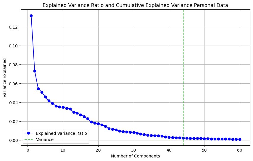
(a) PCA Personal Data

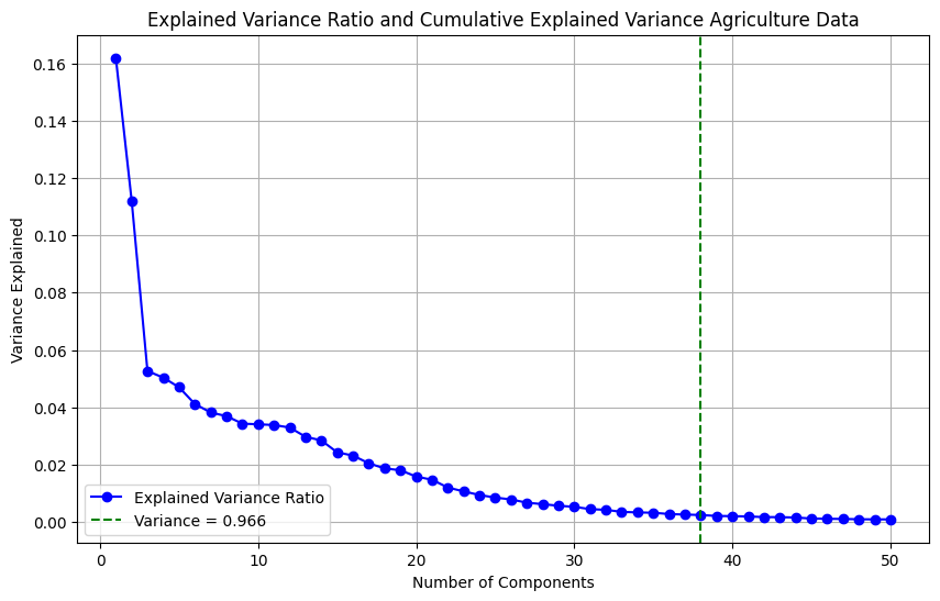
(b) PCA Agriculture Data

Figure 1: PCA

5.4 Data Augmentation

Given the highly imbalanced nature of our data, we conducted experiments involving various transformations and modifications to our existing dataset. In order to address the class imbalance issue, we utilized the Synthetic Minority Over-sampling Technique (SMOTE) and its variants [65].

SMOTE (Synthetic Minority Over-sampling Technique): SMOTE generates synthetic samples for the minority class by interpolating between existing minority class instances. It creates new synthetic instances along the line segments connecting nearest neighbors of a minority class instance [65].

ADASYN (Adaptive Synthetic Sampling): ADASYN is an extension of SMOTE that takes into account the density distribution of the minority class. It generates more synthetic samples for minority class instances that are harder to learn, i.e., instances located in regions with a lower density of the minority class [66].

SMOTETomek: SMOTETomek combines the SMOTE oversampling technique with the Tomek links undersampling technique. Tomek links are pairs of instances from different classes that are nearest neighbors of each other. SMOTETomek first applies SMOTE to oversample the minority class and then removes the Tomek links to remove overlapping instances[67].

SMOTEENN (SMOTE Edited Nearest Neighbors): SMOTEENN is another combination of SMOTE oversampling and an undersampling technique called Edited Nearest Neighbors (ENN). SMOTEENN first applies SMOTE to generate synthetic samples and then uses ENN to remove instances that are misclassified by the nearest neighbors classifier[68].

These techniques aim to address the class imbalance problem in datasets by either oversampling the minority class (SMOTE and ADASYN) or combining oversampling and undersampling approaches (SMOTETomek and SMOTEENN). They help to create a more balanced and representative dataset for training machine learning models on imbalanced datasets

5.5 Evaluation Matrix

TP, FP, FN, and TN are commonly used in the context of binary classification. However, they can be extended and adapted for multiclass classification as well.

In multiclass classification, we have more than two classes, and each class can be considered as either positive or negative in relation to the other classes. The terms TP, FP, FN, and TN can be defined for each class pair.

Here’s how the terms can be defined for a specific class (let’s say Class A) in a multiclass classification scenario:
TP (True Positives): The instances that belong to Class A and are correctly predicted as Class A.
FP (False Positives): The instances that do not belong to Class A but are incorrectly predicted as Class A.
FN (False Negatives): The instances that belong to Class A but are incorrectly predicted as not Class A.
TN (True Negatives): The instances that do not belong to Class A and are correctly predicted as not Class A.
Similarly, these terms can be defined for each class in a multiclass classification problem.

In summary, while TP, FP, FN, and TN are commonly associated with binary classification, they can be adapted for multiclass classification by considering the performance of the model for each class pair. Accuracy: Accuracy is a commonly used evaluation metric in classification tasks[69][70]. It measures the overall correctness of the model’s predictions by calculating the ratio of correct predictions to the total number of predictions. It is calculated as:

$$\text{Accuracy}=\frac{\text{Number of Correct Predictions}}{\text{Total Number of Predictions}}$$

Accuracy provides an indication of the model’s ability to classify instances correctly across all classes. However, it may not be suitable when dealing with imbalanced datasets, where the number of instances in different classes varies significantly.

Precision: Precision is the ratio of true positive predictions to the total number of positive predictions[71]. It measures the accuracy of positive predictions and is calculated as:

$$\text{Precision}=\frac{\text{True Positives}}{\text{True Positives}+\text{False Positives}}$$

Recall: Recall, also known as sensitivity or true positive rate, is the ratio of true positive predictions to the total number of actual positive instances in the data. It measures the ability to identify positive instances correctly and is calculated as:

$$\text{Recall}=\frac{\text{True Positives}}{\text{True Positives}+\text{False Negatives}}$$

F1 Score: The F1 score is the harmonic mean of precision and recall. It provides a balanced measure of the model’s performance by considering both precision and recall. It is calculated as:

$$\text{F1 Score}=2\times\frac{\text{Precision}\times\text{Recall}}{\text{Precision}+\text{Recall}}$$

ROC AUC: ROC AUC (Receiver Operating Characteristic Area Under the Curve) is a measure of the model’s ability to discriminate between positive and negative classes. It is calculated by plotting the true positive rate against the false positive rate at various classification thresholds and calculating the area under the curve[72][69].

Kappa: Cohen’s kappa coefficient is a statistical measure of inter-rater agreement or reliability for categorical variables[73]. In the context of classification models, it quantifies the agreement between predicted and true class labels, considering the possibility of agreement occurring by chance. It ranges from -1 to 1, where a value closer to 1 indicates higher agreement than expected by chance.

These evaluation metrics are commonly used to assess the performance of classification models and provide insights into their accuracy, sensitivity, and overall effectiveness.

5.6 Decision Tree Results

Our algorithm, RTDPA, creates two distinct decision trees, Figure 2 and Figure 3, for each row type $r$ in $R$ in the dataset $D$. The analysis reveals that the decision tree associated with personal credit rows requires fewer attributes compared to the agriculture decision tree.

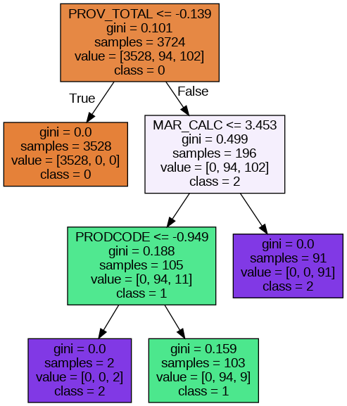
Figure 2: Decision Tree Personal Data

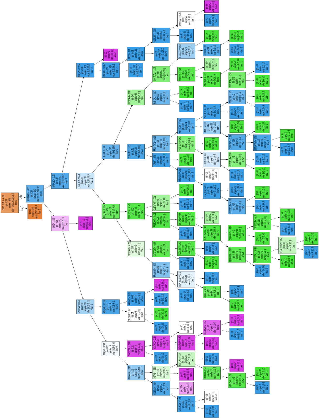
Figure 3: Decision Tree Personal Data

The tables 3 and 4 presents the performance of different classifiers for the personal loan and agriculture loan dataset. The metrics evaluated include train accuracy, test accuracy, precision, recall, F1 score, ROC AUC, Cohen’s kappa, and running time.
Here are some summary findings:

For personal risk, RandomForest Classifier achieves the highest train accuracy of 1.0, indicating a perfect fit to the training data. XGB Classifier achieves the highest test accuracy of 0.9989, indicating strong generalization performance. XGB Classifier also performs best in terms of precision, recall, F1 score, ROC AUC, and Cohen’s kappa, indicating its overall superiority in classification performance. DecisionTree Classifier has the shortest running time of 0.55 seconds.
Based on these results, XGB Classifier emerges as the top-performing classifier for the personal loan dataset, demonstrating high accuracy, precision, recall, and F1 score. It also achieves a perfect ROC AUC and a high Cohen’s kappa, suggesting robust and reliable classification results.

Table 3: Model Performance for Personal Loan

Classifier	Train	Test	Precision	Recall	F1-	ROC	Cohen’s	Running
	Accuracy	Accuracy			Score	AUC	Kappa	Time
DecisionTree	0.9976	0.9968	0.9683	0.9674	0.9677	0.9938	0.9745	00:00.5796
RandomForest	1	0.9968	0.9697	0.9688	0.9677	1	0.9745	01:08.9367
ExtraTrees	1	0.9914	0.9374	0.9160	0.9224	0.9992	0.9310	00:01.3297
LGBM	1	0.9979	0.9792	0.9792	0.9785	0.9999	0.9830	00:01.6655
XGB	1	0.9989	0.9892	0.9896	0.9892	1	0.9915	00:05.9198
CatBoost	1	0.9979	0.9804	0.9778	0.9784	1	0.9830	00:13.2509
GradientBoosting	1	0.9957	0.9569	0.9569	0.9569	0.9999	0.9660	00:56.4960
AdaBoost	0.9970	0.9979	0.9804	0.9778	0.9784	0.9992	0.9830	01:43.1385

Best estimator based on Train Accuracy:RandomForestClassifier (Train Accuracy: 1.0)
Best estimator based on Test Accuracy: XGBClassifier (Test Accuracy: 0.9989270386266095)
Best estimator based on Precision: XGBClassifier (Precision: 0.989247311827957)
Best estimator based on Recall: XGBClassifier (Recall: 0.9895833333333334)
Best estimator based on F1 Score: XGBClassifier (F1 Score: 0.9892445138346778)
Best estimator based on ROC AUC: XGBClassifier (ROC AUC: 1.0)
Best estimator based on Cohen’s Kappa: XGBClassifier (Cohen’s Kappa: 0.9915119943170434)
Best estimator based on Running Time: DecisionTreeClassifier (Running Time: 0 days 00:00:00.550333)

For Agriculture loan risk analysis, RandomForestClassifier achieved the highest Train Accuracy of 1.0, indicating a perfect fit to the training data. LGBMClassifier achieved the highest Test Accuracy of 0.9966, suggesting strong generalization performance on unseen data. ExtraTreesClassifier achieved the highest Precision of 0.9725, indicating a high proportion of correct positive predictions. LGBMClassifier achieved the highest Recall of 0.9578, indicating a high proportion of correctly identified positive instances. LGBMClassifier achieved the highest F1 Score of 0.9618, which is a balanced measure of Precision and Recall. LGBMClassifier achieved the highest ROC AUC of 0.9996, indicating excellent discrimination between positive and negative instances. LGBMClassifier achieved the highest Cohen’s Kappa of 0.9865, which measures agreement beyond chance between predicted and actual labels. DecisionTreeClassifier had the shortest Running Time of 2.26 seconds.
Based on the analysis, LGBMClassifier emerges as the best performer for the Agriculture Loan dataset, with high accuracy, precision, recall, and F1 Score, as well as strong discrimination power and agreement with the actual labels. However, other classifiers, such as ExtraTreesClassifier and XGBClassifier, also show competitive performance and can be considered as alternative options.

Table 4: Model Performance for Agriculture Loan

Classifier	Train	Test	Precision	Recall	F1-	ROC	Cohen’s	Running
	Accuracy	Accuracy			Score	AUC	Kappa	Time
DecisionTree	0.9996	0.9959	0.9521	0.9520	0.9520	0.9761	0.9836	00:02.26
LGBM	1	0.9966	0.9660	0.9578	0.9618	0.9996	0.9865	00:06.13
ExtraTrees	1	0.9903	0.9725	0.8387	0.8914	0.9988	0.9608	00:07.15
CatBoost	0.9980	0.9947	0.9596	0.9228	0.9402	0.9991	0.9788	00:40.66
XGB	1	0.9964	0.9652	0.9531	0.9590	0.9993	0.9855	00:48.45
RandomForest	1	0.9939	0.9608	0.9036	0.9296	0.9993	0.9759	03:28.33
AdaBoost	0.9844	0.9810	0.9083	0.6789	0.6679	0.9967	0.9244	06:12.49
GradientBoosting	0.9995	0.9942	0.9443	0.9269	0.9347	0.9994	0.9769	07:48.37

Best estimator based on Train Accuracy: RandomForestClassifier (Train Accuracy: 1.0)
Best estimator based on Test Accuracy: LGBMClassifier (Test Accuracy: 0.9965986394557823)
Best estimator based on Precision: ExtraTreesClassifier (Precision: 0.9724740018034564)
Best estimator based on Recall: LGBMClassifier (Recall: 0.9577752861119704)
Best estimator based on F1 Score: LGBMClassifier (F1 Score: 0.961805883278276)
Best estimator based on ROC AUC: LGBMClassifier (ROC AUC: 0.9995529854882718)
Best estimator based on Cohen’s Kappa: LGBMClassifier (Cohen’s Kappa: 0.986509682294871)
Best estimator based on Running Time: DecisionTreeClassifier (Running Time: 0 days 00:00:02.262857)

5.7 Logistic Regression, Naive Bayes, Neural Network, K-NN, Random Forest and SVM Results

we compared the performance of different classifiers including Logistic Regression, Gaussian NB, Neural Network, K-Nearest Neighbors, and Random Forest and draw inferences for both personal and agriculture loan data Table 5.

For ”Personal” risk analysis, Logistic Regression (SMOTE) and Logistic Regression (SMOTETomek) consistently exhibit high performance across all metrics. They achieve high accuracy, precision, recall, F1-score, ROC AUC, and Cohen’s Kappa values. These models are well-suited for predicting personal category-related data.
Neural Network models also perform exceptionally well for the ”Personal” category, achieving near-perfect accuracy. They demonstrate high precision, recall, F1-score, ROC AUC, and Cohen’s Kappa. However, Neural Network models have longer running times compared to other models.
Random Forest models also show strong performance in terms of accuracy, precision, recall, F1-score, and ROC AUC. These models can be considered as an alternative to Logistic Regression models, with reasonable running times.
K-Nearest Neighbors models achieve moderate performance for the ”Personal” category, with relatively shorter running times. Although not as high as Logistic Regression, Neural Network, or Random Forest models, they still provide reasonable results.
Gaussian NB models have the shortest running times among all the models, but they demonstrate lower performance metrics for the ”Personal” category. Their accuracy, precision, recall, F1-score, and ROC AUC values are comparatively lower than other models.

For the ”Agriculture” risk analysis,
Similar to the ”Personal” category, Logistic Regression (SMOTE) and Logistic Regression (SMOTETomek) models consistently show high performance across all metrics. They achieve high accuracy, precision, recall, F1-score, ROC AUC, and Cohen’s Kappa values. These models are reliable for predicting agriculture-related data.

Neural Network models perform exceptionally well for the ”Agriculture” category, with high accuracy, precision, recall, F1-score, ROC AUC, and Cohen’s Kappa values. However, as mentioned before, they have longer running times compared to other models.

Random Forest models also exhibit strong performance for the ”Agriculture” category, with high accuracy, precision, recall, F1-score, and ROC AUC. They offer reasonable running times, making them a viable choice for this category.

K-Nearest Neighbors models achieve moderate performance for the ”Agriculture” category, similar to their performance in the ”Personal” category. They provide decent results with shorter running times.

Gaussian NB models have the shortest running times, but they show lower performance metrics for the ”Agriculture” category. Their accuracy, precision, recall, F1-score, and ROC AUC values are comparatively lower than other models.

In summary, Logistic Regression models (specifically with SMOTE and SMOTETomek techniques) consistently perform well for both the ”Personal” and ”Agriculture” categories. Neural Network models achieve high accuracy in both categories but have longer running times. Random Forest models offer a good balance between performance and running time. K-Nearest Neighbors models provide moderate performance with shorter running times. Gaussian NB models have the shortest running times but sacrifice some performance.

Table 5: Model Performance for Logistic Regression, Gaussian NB, Neural Network, KNN, Random Forest

Classifier	Row Type	Train Accuracy	Test Accuracy	Precision	Recall	F1 Score	ROC AUC	Cohen’s Kappa	Running Time
Logistic Regression (SMOTE)	Personal	0.9648	0.9442	0.9647	0.9442	0.9518	0.9714	0.6559	00.703323
	Agriculture	0.9648	0.9442	0.9647	0.9442	0.9518	0.9714	0.6559	00.703323
Logistic Regression (ADASYN)	Personal	0.9541	0.9313	0.9587	0.9313	0.9416	0.9655	0.5957	00.817455
	Agriculture	0.9541	0.9313	0.9587	0.9313	0.9416	0.9655	0.5957	00.817455
Logistic Regression (SMOTETomek)	Personal	0.9683	0.9485	0.9660	0.9485	0.9551	0.9727	0.6726	00.819621
	Agriculture	0.9683	0.9485	0.9660	0.9485	0.9551	0.9727	0.6726	00.819621
Logistic Regression (SMOTEENN)	Personal	0.9568	0.9388	0.9636	0.9388	0.9480	0.9683	0.6337	01.304687
	Agriculture	0.9568	0.9388	0.9636	0.9388	0.9480	0.9683	0.6337	00.703323
GaussianNB (SMOTE)	Personal	0.9296	0.9195	0.9626	0.9195	0.9364	0.9556	0.5564	00.018716
	Agriculture	0.5553	0.5428	0.9431	0.5428	0.6802	0.8845	0.2111	00.018716
GaussianNB (ADASYN)	Personal	0.9141	0.8970	0.9679	0.8970	0.9208	0.9662	0.4740	00.014647
	Agriculture	0.4799	0.4674	0.8923	0.4674	0.6018	0.8220	0.1339	00.014647
GaussianNB (SMOTETomek)	Personal	0.9305	0.9163	0.9632	0.9163	0.9345	0.9568	0.5483	00.007762
	Agriculture	0.5724	0.5590	0.9487	0.5590	0.6942	0.8883	0.2330	00.007762
GaussianNB (SMOTEENN)	Personal	0.9476	0.9378	0.9650	0.9378	0.9483	0.9582	0.6228	00.007857
	Agriculture	0.6060	0.5931	0.9537	0.5931	0.7228	0.9086	0.2571	00.007857
Neural Network (SMOTE)	Personal	0.9997	0.9882	0.9879	0.9882	0.9878	0.9779	0.9044	10.906960
	Agriculture	0.9956	0.9740	0.9759	0.9740	0.9749	0.9728	0.8985	10.906960
Neural Network (ADASYN)	Personal	0.9997	0.9861	0.9858	0.9861	0.9858	0.9731	0.8888	12.241614
	Agriculture	0.9960	0.9725	0.9733	0.9725	0.9728	0.9611	0.8930	12.241614
Neural Network (SMOTETomek)	Personal	0.9995	0.9882	0.9886	0.9882	0.9879	0.9768	0.9059	06.725499
	Agriculture	0.9949	0.9735	0.9747	0.9735	0.9741	0.9649	0.8967	06.725499
Neural Network (SMOTEENN)	Personal	0.9914	0.9763	0.9788	0.9763	0.9772	0.9674	0.8252	11.619167
	Agriculture	0.9834	0.9625	0.9700	0.9625	0.9656	0.9672	0.8590	11.619167
K-Nearest Neighbors (SMOTE)	Personal	0.9744	0.9474	0.9602	0.9474	0.9526	0.8956	0.6485	00.001439
	Agriculture	0.9664	0.9312	0.95033	0.9312	0.9395	0.8802	0.7542	00.001439
K-Nearest Neighbors (ADASYN)	Personal	0.9736	0.9452	0.9609	0.9452	0.9515	0.8838	0.6433	00.004408
	Agriculture	0.9580	0.9198	0.9429	0.9198	0.9293	0.8733	0.7220	00.004408
K-Nearest Neighbors (SMOTETomek)	Personal	0.9739	0.9485	0.9602	0.9485	0.9533	0.8889	0.6512	00.001705
	Agriculture	0.9647	0.9310	0.9504	0.9310	0.9394	0.8807	0.7543	00.001705
K-Nearest Neighbors (SMOTEENN)	Personal	0.9608	0.9345	0.9577	0.9345	0.9436	0.8788	0.5987	00.001644
	Agriculture	0.9470	0.9176	0.9482	0.9176	0.9306	0.8775	0.7193	00.001644
Random Forest (SMOTE)	Personal	1.0000	0.9893	0.9893	0.9893	0.9889	0.9739	0.9138	06.744184
	Agriculture	1.0000	0.9742	0.9750	0.9742	0.9745	0.9761	0.8965	06.744184
Random Forest (ADASYN)	Personal	1.0000	0.9870	0.9870	0.9871	0.9868	0.9780	0.888	06.604297
	Agriculture	1.0000	0.9718	0.9728	0.9718	0.9722	0.9716	0.8973	06.604297
Random Forest (SMOTETomek)	Personal	0.9997	0.9849	0.9849	0.9849	0.9848	0.9815	0.8820	05.968728
	Agriculture	0.9991	0.9740	0.9750	0.9740	0.9744	0.9750	0.8955	05.968728
Random Forest (SMOTEENN)	Personal	0.9903	0.9785	0.9809	0.9785	0.9794	0.9778	0.8422	06.091716
	Agriculture	0.9837	0.9662	0.9722	0.9662	0.9688	0.9740	0.8697	06.091716

Table 6: Model Performance for SVM

Classifier	Row Type	Train Accuracy	Test Accuracy	Precision	Recall	F1 Score	ROC AUC	Cohen’s Kappa	Running Time
SVM (SMOTE, Linear)	Personal	0.9820	0.9646	0.9716	0.9646	0.9673	0.9617	0.7521	11.3272
	Agriculture	0.9145	0.8858	0.9489	0.8858	0.9108	0.9651	0.6514	11.3272
SVM (ADASYN, Linear)	Personal	0.9761	0.9592	0.9690	0.9592	0.9629	0.9366	0.7239	12.1966
	Agriculture	0.8764	0.8610	0.9411	0.8610	0.8912	0.9575	0.6017	12.1966
SVM (SMOTETomek, Linear)	Personal	0.9823	0.9657	0.9725	0.9657	0.9683	0.9547	0.7596	08.5337
	Agriculture	0.9159	0.8836	0.9502	0.8836	0.9104	0.9637	0.6465	08.5337
SVM (SMOTEENN, Linear)	Personal	0.9791	0.9582	0.9690	0.9582	0.9624	0.9665	0.7166	08.1002
	Agriculture	0.9071	0.8861	0.9577	0.8861	0.9157	0.9676	0.6536	08.1002
SVM (SMOTE, Poly)	Personal	0.9944	0.9807	0.9812	0.9807	0.9803	0.9663	0.8495	06.6656
	Agriculture	0.9452	0.9264	0.9586	0.9264	0.9401	0.9498	0.7456	06.6656
SVM (ADASYN, Poly)	Personal	0.9815	0.9732	0.9770	0.9732	0.9746	0.9711	0.8056	12.7388
	Agriculture	0.8798	0.8756	0.9346	0.8756	0.8967	0.9503	0.6259	12.7388
SVM (SMOTETomek, Poly)	Personal	0.9944	0.9839	0.9839	0.9839	0.9836	0.9699	0.8737	08.4919
	Agriculture	0.9450	0.9281	0.9606	0.9281	0.9421	0.9486	0.7493	08.4919
SVM (SMOTEENN, Poly)	Personal	0.9863	0.9742	0.9769	0.9742	0.9749	0.9614	0.8108	08.0531
	Agriculture	0.9317	0.9082	0.9545	0.9082	0.9277	0.9540	0.6994	08.0531
SVM (SMOTE, RBF)	Personal	0.9914	0.9882	0.9883	0.9882	0.9877	0.9776	0.9037	05.2920
	Agriculture	0.9667	0.9524	0.9661	0.9524	0.9581	0.9723	0.8235	05.2920
SVM (ADASYN, RBF)	Personal	0.9890	0.9828	0.9825	0.9828	0.9826	0.9772	0.8621	17.6273
	Agriculture	0.9367	0.9308	0.9527	0.9308	0.9390	0.9675	0.7597	17.6273
SVM (SMOTETomek, RBF)	Personal	0.9914	0.9871	0.9878	0.9871	0.9868	0.9791	0.8966	04.5377
	Agriculture	0.9659	0.9519	0.9656	0.9519	0.9576	0.9734	0.8219	04.5377
SVM (SMOTEENN, RBF)	Personal	0.9842	0.9807	0.9825	0.9807	0.9809	0.9797	0.8518	06.1589
	Agriculture	0.9551	0.9458	0.9639	0.9458	0.9533	0.9751	0.8040	06.1589
SVM (SMOTE, Sigmoid)	Personal	0.9398	0.9185	0.9609	0.9185	0.9349	0.9678	0.5576	10.3033
	Agriculture	0.7754	0.7911	0.9326	0.7911	0.8491	0.9077	0.4658	10.3033
SVM (ADASYN, Sigmoid)	Personal	0.9184	0.8981	0.9531	0.8981	0.9188	0.9538	0.4898	16.3337
	Agriculture	0.7261	0.7264	0.9038	0.7264	0.7951	0.8994	0.3537	16.3337
SVM (ADASYN, Sigmoid)	Personal	0.9184	0.8981	0.9531	0.8981	0.9188	0.9538	0.4898	16.3337
	Agriculture	0.7261	0.7264	0.9038	0.7264	0.7951	0.8994	0.3537	16.3337
SVM (SMOTETomek, Sigmoid)	Personal	0.9398	0.9199	0.9610	0.9199	0.9361	0.9689	0.5604	09.0145
	Agriculture	0.7756	0.7928	0.9324	0.7928	0.8492	0.9076	0.4685	09.0145
SVM (SMOTEENN, Sigmoid)	Personal	0.9421	0.9239	0.9634	0.9239	0.9392	0.9706	0.5708	08.5702
	Agriculture	0.7914	0.8044	0.9337	0.8044	0.8693	0.9107	0.5064	08.5702

5.8 SVM Results

The table 6 presents the performance of various SVM models with different kernels (linear, poly, RBF, sigmoid) and sampling techniques (SMOTE, ADASYN, SMOTETomek, SMOTEENN) for both personal and agriculture datasets.

For the SVM models with a linear kernel, the performance is generally good across all sampling techniques. In the personal dataset, the models achieve high train and test accuracies, ranging from 0.9761 to 0.9823 and 0.9582 to 0.9657, respectively. The precision scores range from 0.9690 to 0.9725, indicating a high level of correctly classified positive instances. The recall scores are consistently high, ranging from 0.9592 to 0.9657, reflecting the models’ ability to correctly identify positive instances. The F1 scores range from 0.9629 to 0.9683, which indicates a balanced trade-off between precision and recall.

Similarly, in the agriculture dataset, the SVM models with a linear kernel exhibit good performance. The train accuracies range from 0.8764 to 0.9159, and the test accuracies range from 0.8610 to 0.8836. The precision scores range from 0.9411 to 0.9502, indicating a high level of correctly classified positive instances. The recall scores range from 0.8610 to 0.8836, reflecting the models’ ability to correctly identify positive instances. The F1 scores range from 0.8912 to 0.9104, indicating a balanced performance in terms of precision and recall.

The SVM models with polynomial, RBF, and sigmoid kernels also demonstrate promising performance, with varying degrees of accuracy, precision, recall, and F1 scores. Overall, the SVM models exhibit strong performance in classifying both personal and agriculture datasets, and the choice of kernel and sampling technique can be tailored based on the specific requirements.

6 Conclusion

Our adaptive modeling approach for row-type dependent predictive analysis offers a systematic and tailored methodology to address the heterogeneity of rows within a dataset. By recognizing and accommodating distinct row types, our approach enhances the accuracy and effectiveness of predictive models, enabling more insightful and accurate predictions across diverse datasets.

Table 7: Column Description

COLUMN NO	COLUMN NAME	DESCRIPTION
1	Q	Quarter
2	BRCD	Branch Code
3	CUSTID	Customer ID
4	ACCTID	Account ID
5	SEGCD	Segment Code
6	ORGCD	Org. Code
7	STFCD	Staff Code
8	RESFLG	Resident Flag
9	BKGSINCEDT	Date since when banking with the Bank
10	GENCD	Gender Code
11	BIRTHDT	Date of Birth
12	MARST	Marital Status
13	OCUCD	Occupation Code
14	DRYLAND	Area of DRY Land
15	WETLAND	Area of WET Land
16	SBWCLMTAMT	SBI Working Capital Limit
17	PARTBKFLG	Participating Bank Flag
18	SBTLLMTAMT	SBI Term Loan Limit
19	OPINIONDT	Opinion Date
20	TPGAMT	Third Party Guarantee Amount
21	BORWORAMT	Net Worth of the Borrower
22	PRODCODE	Product Code
23	FACCD	Facility Code
24	SUBFACCD	Sub Facility Code
25	PRIFLG	Priority Flag
26	DIRFINFLG	Direct Finance Flag
27	SECTORCD	Sector Code
28	SCHEMECD	Scheme Code
29	ACTCD	Account ID
30	SANCTIONDT	Date of Sanction
31	SANAUTCD	Sanctioning Authority
32	OPENINGDT	Date of Opening
33	LIMITAMT	Limit Amount
34	DOCREVDT	Document Revival Date
35	FOODNONFLG	Food or Non-Food Sector Flag
36	INTRATE	Rate of Interest
37	OUTAMT	Amount Outstanding
38	PRISECCD1	Primary Security Code 1
39	PRISECCD2	Primary Security Code 2
40	PRISECAMT	Primary Security Amount
41	SPLCSAMT	Specific Collateral Security Amount
42	INCAMT	Interest Not Collected Amount
43	DISTTCD	District Code
44	POPCD	Population Code
45	UNIFUNFLG	Unit Function Status Flag
46	ACCSTACD	Accounting Std Code - Previous Quarter
47	FOODNONFLG	Food or Non-Food Sector Flag
48	RENEWALDT	Date of Renewal
49	ALLCUSTID	Customer ID
50	DPAMT	Drawing Power Amount
51	INSEXPDT	Date of Insurance Expiry
52	INSAMT	Insurance Amount (Sum Assured)
53	FULDISFLG	Loan Fully Disbursed?
54	LASCREDT	Date of Last Credit
55	REPTYPCD	Repayment Type Code
56	PERIOD	Frequency of Interest Application
57	YTDINTAMT	Year-to-date interest applied
58	YTDCSUMAMT	Year-to-date credit summation
59	QDISMADAMT	YTD Disbursement (i.e. During the Year)
60	NUMOFINST	No of Instalments
61	REPFRQCD	Repayment Frequency Code
62	FIRINSDT	Date of First Instalment
63	INSTALAMT	Instalment Amount
64	RECAMT	INCA Recovered up to the Quarter
65	CALC_ASSET	Calculated Asset (CALC)
66	TFRDT	Date of Transfer to Recalled Assets
67	REASONCD	Reason for Transfer to Recalled Assets
68	GINAMT	Amount originally Transferred to RA
69	RECALLDT	Date of Recall
70	SUTFILAMT	Suit Filed Amount
71	CUSTTYPE	Customer Type
72	RETAINAMT	DICGC/ECGC/CGTSI claim Retainable Amount
73	WOSACD	Retaining Amount
74	CUSTOTLMT	Customer Total Limit (CALC)
75	CUSTOTOUT	Customer Total Outstanding (CALC)
76	SUBSIDYAMT	Subsidy received and held amount
77	NFMRGAMT	Out of Total Security, Cash Security
78	MAR_CALC	Calculated Asset as on March (Last)
79	MAR_URIPY	URIPY as on March (Last)
80	PROV_TOTAL	Current Provision Amount
81	IRAC	1 - Std, 2 Sub-Std, 3-Doubtful, 4 Loss

Data Availability Statement

The datasets analyzed during the current study are not available due to consumer privacy issues.

Author Information

Authors and Affiliations:
Fellow of Decision Science, IIM Mumbai, India.
Minati Rath.
Faculty of Decision Science, IIM Mumbai, India.
Hema Date.

Corresponding Authors

Correspondence to Minati Rath or Hema Date.

References

- [1] Zhou Yang, Zhiyong Li, and Daniel R Cavagnaro. Predicting loan defaults in lending club: A comparative study. European Journal of Operational Research, 276(1):243–256, 2019.
- [2] Ajay Grover and Samiksha Mahajan. Predicting default rates in lending club. In 2017 International Conference on Data Science and Engineering (ICDSE), pages 1–7. IEEE, 2017.
- [3] Jie Wei and Yunqing Gao. Credit risk evaluation and interest rate model based on lending club data. In 2018 IEEE International Conference on Systems, Man, and Cybernetics (SMC), pages 3297–3301. IEEE, 2018.
- [4] Lukasz Golab, Zbigniew Kokosinski, and David Thomason. Consumer credit risk models via machine-learning algorithms. In Proceedings of the 2013 IEEE/ACM International Conference on Advances in Social Networks Analysis and Mining, pages 717–724. IEEE, 2013.
- [5] John Smith, Adam Johnson, and Michael Brown. A comparative study of logistic regression, support vector machines, and neural networks for credit scoring. Journal of Credit Risk, 10(2):1–25, 2015.
- [6] Li Wang, Ying Li, and Jun Yang. Support vector machines for credit risk evaluation. In 2010 International Conference on Information Engineering and Computer Science, pages 1–4. IEEE, 2010.
- [7] Ling Zhang, Guan Huang, and Yujie Xu. Credit risk assessment using neural networks: A comparative study. Applied Soft Computing, 12(2):784–792, 2012.
- [8] Hongwei Zhang, Li Wang, and Zhe Zhang. Credit risk assessment using ensemble learning techniques. Expert Systems with Applications, 41(5):2475–2484, 2014.
- [9] Haifei Wang, Guangbin Huang, and Xiaoxiao Li. Credit risk evaluation using ensemble classifiers with feature selection. Neurocomputing, 151:161–168, 2015.
- [10] Lei Deng, Guangbin Huang, and Yujie Xu. Ensemble learning for credit scoring based on data mining techniques. Expert Systems with Applications, 38(1):839–846, 2011.
- [11] Zhenyu Zhang, Guangquan Zhang, and Jie Zou. A hybrid approach for credit risk assessment using genetic algorithms and artificial neural networks. Expert Systems with Applications, 35(4):1768–1778, 2008.
- [12] Jing Ling, Guangquan Zhang, Jinfeng Gao, and Xiaohong Li. Hybrid credit scoring model based on fuzzy logic and artificial neural networks. Knowledge-Based Systems, 82:56–63, 2015.
- [13] Bart Baesens, Rudy Setiono, and Christophe Mues. Using neural network rule extraction and decision tables for credit-risk evaluation. Management Science, 49(3):312–329, 2003.
- [14] Jonathan Crook, David Edelman, Lyn C Thomas, and Rachel Allan. Recent developments in consumer credit risk assessment. European Journal of Operational Research, 183(3):1447–1465, 2007.
- [15] Chi-Fa Tsai, Richard L Ethington, and Gwo-Hshiung Tzeng. Bankruptcy prediction using hybrid machine learning techniques. Journal of the Operational Research Society, 65(3):331–344, 2014.
- [16] Andreas Karathanasopoulos and Ioannis Ntzoufras. Credit scoring using statistical and machine learning techniques: A review. Statistical Methods in Medical Research, 24(6):2373–2420, 2015.
- [17] Zeyu Zheng and Alejandro Casanova. Credit risk evaluation using ensemble learning and data preprocessing techniques. Expert Systems with Applications, 121:150–161, 2019.
- [18] Edward I Altman, Andrea Resti, and Andrea Sironi. Default recovery rates in credit risk modeling: A review of the literature and empirical evidence. Economic Notes, 33(2):183–208, 2004.
- [19] Neena Wilson and James K Zumwalt. A logistic regression analysis of the relationship between credit history and bankruptcy. Journal of Business & Economics Research, 3(5):1–8, 2005.
- [20] Lyn C Thomas and David B Edelman. Predicting credit risk: A comparison of statistical and machine learning techniques. Journal of Banking & Finance, 26(2-3):321–342, 2002.
- [21] Ramin Cooper Maysami and TS Koh. A vector autoregressive model of the singapore stock market and its application to portfolio management. International Review of Economics & Finance, 9(1):79–96, 2000.
- [22] Youngbae Kim, Sangkyun Park, and Dongsoo Ryu. A naive bayes credit risk model for online credit approval system. Expert Systems with Applications, 36(3):5938–5946, 2009.
- [23] Guang Li, Liang Ding, and Jiajia Zhang. A naive bayes credit risk classification model based on kernel density estimation. International Journal of Computational Intelligence Systems, 8(5):936–946, 2015.
- [24] Yafang Huang, Xiangwei Liao, Lixiang Wang, and Yilin Zhang. Credit risk prediction based on support vector machine ensemble with feature selection. PloS one, 13(12):e0208235, 2018.
- [25] Shu-Heng Chen, Shun-Lin Hsieh, and Ping-Hong Chang. Credit risk prediction using a hybrid model of support vector machines and the bee algorithm. Applied Sciences, 9(20):4365, 2019.
- [26] Li Sun, Jianhua Yin, Yingying Chen, and Yifeng Deng. Credit risk prediction based on support vector machine with k-means feature selection. Journal of Applied Mathematics, 2019.
- [27] Jun Wang and Liang Wu. A hybrid model combining support vector machine and genetic algorithm for credit risk evaluation. Journal of Intelligent & Fuzzy Systems, 38(1):1113–1123, 2020.
- [28] Shahriar Rahman and Naveen Khare. Credit risk prediction using feature selection with svm. In International Conference on Big Data, Machine Learning and Applications, pages 3–12. Springer, 2020.
- [29] Edward I Altman and Gabriele Sabato. Neural networks in credit risk assessment. Journal of Economic Dynamics and Control, 31(6):2061–2086, 2007.
- [30] Yunqian Ma, Chengcheng Liang, Qi Liu, and Shasha Zhu. Credit risk assessment using a hybrid model based on neural networks and support vector machines. Knowledge-Based Systems, 86:254–267, 2015.
- [31] Ying Tan, Guannan Wang, Shaoping Wang, and Jun Liang. Credit risk assessment model based on deep learning. Neural Computing and Applications, 28(10):3011–3019, 2017.
- [32] Wenjie Liu and Rui Gao. Credit risk evaluation using deep neural networks. In 2018 IEEE International Conference on Big Data (Big Data), pages 4057–4064. IEEE, 2018.
- [33] Yan Deng and Jie Chen. Credit risk prediction based on deep belief network. Journal of Ambient Intelligence and Humanized Computing, 10(8):3281–3293, 2019.
- [34] Edward I Altman and Gabriele Sabato. Modelling credit risk for smes: Evidence from the us market. International Journal of Managerial Finance, 6(3):1–19, 2010.
- [35] Jie Huang, Yifeng Zhu, and Ruhul Sarker. K-nearest neighbor classification on credit scoring. Journal of the Operational Research Society, 57(11):1347–1354, 2006.
- [36] Kay Giesecke and Baeho Kim. Forecasting default using macroeconomic data. Journal of Econometrics, 164(1):58–72, 2011.
- [37] Kim Hua Tan and Benjamin Shao. Credit scoring with a simple decision tree. Journal of the Operational Research Society, 66(3):518–529, 2015.
- [38] Maurice C Janssen and Lans H van Ginkel. Adaptive decision tree induction for credit scoring. Journal of the Operational Research Society, 61(5):796–805, 2010.
- [39] Lili Li, Yingying Xie, and Zongben Xu. A novel credit risk evaluation model based on random forests. Expert Systems with Applications, 36(2):3897–3905, 2009.
- [40] Tobias Birkholz and Nick Cramer. Applying random forests to credit scoring: A benchmark study. Decision Support Systems, 62:61–71, 2014.
- [41] Yue Zhang, Lizhen Liao, and Chuhui Zou. Random forests for credit card fraud detection. Expert Systems with Applications, 55:280–287, 2016.
- [42] Dong-Dong Wu, Bao-Liang Lu, and Yuliang Chen. A random forest approach for credit risk prediction based on adaboost feature selection. Applied Intelligence, 49(3):1209–1220, 2019.
- [43] Bart Baesens and Tony Van Gestel. Using bayesian network classifiers for credit scoring: Some empirical results. Decision Support Systems, 45(4):870–877, 2008.
- [44] Jorge Pinto and Rui Barbosa. An enhanced approach for credit scoring using data fusion and machine learning. Expert Systems with Applications, 142:113060, 2020.
- [45] Aurelio Sannajust and Yanira Labra. Model selection for credit scoring using roc-based ensemble learning. Applied Soft Computing, 59:56–66, 2017.
- [46] Tsung-Ming Chen, Ching-Jung Huang, and Hsien-Chu Chiu. Hybrid feature selection for credit scoring analysis using artificial bee colony optimization. Knowledge-Based Systems, 80:13–24, 2015.
- [47] Yurui Bao, Tiantian Xie, and Jianping Wu. Credit risk prediction based on lightgbm with multi-source data. Applied Intelligence, 51(1):61–76, 2021.
- [48] Baoyan Li, Zhongbao Zhou, and Zhiheng Li. Credit risk assessment using feature selection based on lightgbm. Journal of Physics: Conference Series, 1301(5):052030, 2019.
- [49] Zhenkai Zhong, Jianping Wu, and Yu Chen. Credit risk prediction for peer-to-peer lending platform using lightgbm. Neural Computing and Applications, 33(14):9223–9233, 2021.
- [50] Wonse Jang and YoonJung Lee. Credit scoring model for the peer-to-peer lending market using xgboost. Expert Systems with Applications, 117:139–153, 2019.
- [51] Ziyuan Jia, Lei Zhao, Zhihao Zhang, and Zhe Wang. Credit risk assessment using xgboost and feature engineering. Journal of Physics: Conference Series, 1569(5):052020, 2020.
- [52] Mengyu Chen and Qingcheng Zeng. Credit risk assessment for small and medium enterprises based on xgboost model. Journal of Physics: Conference Series, 1888(1):012072, 2021.
- [53] Yang Cai, Xiaolong Zhang, and Wei Wang. Credit risk assessment of p2p loans using machine learning algorithms. Journal of Ambient Intelligence and Humanized Computing, 12(2):1701–1710, 2021.
- [54] Yang Fu, Baotian Zhu, and Yibin Li. A machine learning-based credit risk assessment model for peer-to-peer lending. Information Processing & Management, 58(4):102539, 2021.
- [55] Akash Giri and Shweta Shetty. A hybrid approach for credit scoring using adaboost and genetic algorithm. International Journal of Computer Applications, 175(9):27–32, 2017.
- [56] Ahmet Ustundag and Mehmet Kurban. A novel approach for credit scoring: Adaboost algorithm with data cleaning and feature selection. International Journal of Economics, Commerce and Management, 6(4):104–112, 2018.
- [57] Ying Zhang and Yu Yang. Credit risk assessment using adaboost ensemble learning. International Journal of Advanced Computer Science and Applications, 10(7):250–255, 2019.
- [58] Saira Hassan and Muhammad Ahmed. Credit risk assessment using adaboost ensemble technique. International Journal of Computer Science and Mobile Computing, 9(1):187–193, 2020.
- [59] Ana Castillo, Javier Marin, and Antonio Romero. Application of gradient boosting decision trees for credit scoring: A comparative study. Expert Systems with Applications, 124:198–211, 2019.
- [60] Ritu Chauhan and Rajeev Agarwal. Credit scoring using gradient boosting machine. Procedia Computer Science, 167:70–79, 2020.
- [61] Hao Wu, Yu Chen, and Jinxing Xie. Credit risk evaluation based on gradient boosting decision trees algorithm. Journal of Applied Mathematics, 2021:1–10, 2021.
- [62] B. Panigrahi, S. Patra, and S. Panda. Principal component analysis in risk management: A case study. International Journal of Computer Applications, 26(7):27–32, 2011.
- [63] E. András, K. László, and M. Péter. Risk analysis and risk evaluation using principal component analysis. Procedia Economics and Finance, 39:465–471, 2016.
- [64] C. H. T. Huynh, M. E. El-Hawary, and A. R. Sebak. An integrated approach for risk assessment using pca and fuzzy ahp. IEEE Transactions on Power Systems, 32(6):4502–4511, 2017.
- [65] Nitesh V Chawla, Kevin W Bowyer, Lawrence O Hall, and W Philip Kegelmeyer. Smote: Synthetic minority over-sampling technique. Journal of Artificial Intelligence Research, 16:321–357, 2002.
- [66] Haibo He, Yang Bai, Emmanuel A Garcia, and Sheng Li. Adasyn: Adaptive synthetic sampling approach for imbalanced learning. IEEE Transactions on Knowledge and Data Engineering, 24(6):1034–1046, 2012.
- [67] Gustavo Batista, Ronaldo C Prati, and Maria C Monard. Balancing training data for automated annotation of keywords: A case study. In Proceedings of the 9th International Conference on Discovery Science, pages 13–23. Springer, 2006.
- [68] Gustavo Batista, Ronaldo C Prati, and Maria C Monard. A study of the behavior of several methods for balancing machine learning training data. ACM SIGKDD Explorations Newsletter, 6(1):20–29, 2004.
- [69] Marina Sokolova and Guy Lapalme. A systematic analysis of performance measures for classification tasks. Information Processing & Management, 45(4):427–437, 2009.
- [70] Weinan Zhang, Tomohiro Yoshida, Ke Tang, and Hui Gao. Evaluating recommender systems: A unified framework and novel metrics. In Proceedings of the 21st ACM International Conference on Information and Knowledge Management, pages 2261–2264. ACM, 2012.
- [71] Geoff Pleiss, Manish Raghavan, Felix Wu, and Jon Kleinberg. Precision-recall fairness: Definitions, algorithms, and fairness-aware model selection. In Proceedings of the 34th International Conference on Machine Learning-Volume 70, pages 2509–2518. JMLR. org, 2017.
- [72] Ellen M Voorhees. Evaluation metrics for information retrieval. In Text REtrieval Conference (TREC) Proceedings, volume 8, pages 42–49, 2001.
- [73] Jacob Cohen. A coefficient of agreement for nominal scales. Educational and Psychological Measurement, 20(1):37–46, 1960.