Extending Neural Network Verification to a Larger Family of Piece-wise Linear Activation Functions

Abstract

In this paper, we extend an available neural network verification technique to support a wider class of piece-wise linear activation functions. Furthermore, we extend the algorithms, which provide in their original form exact respectively over-approximative results for bounded input sets represented as star sets, to allow also unbounded input sets. We implemented our algorithms and demonstrated their effectiveness in some case studies.

1 Introduction

In the area of artificial intelligence, feed-forward neural networks (FNNs) [33] enjoy increasing popularity. FNNs can be trained to learn a function $f:\mathbb{R}^{n}\rightarrow\mathbb{R}^{m}$ from a set of input-output samples, and predict outputs also for previously unseen inputs. This way, FNNs can tackle problems that would otherwise require very complex solutions [46].

Nowadays, a wide range of applications use FNNs, such as autonomous vehicles [32], speech- and object-recognition systems [23, 14] or robot vision [34], just to mention a few. While FNNs are impressively effective, their reliability in safety-critical situations is still questionable [10, 17, 25]. Hence, verification methods play an important role in providing guarantees about their behavior. In this work, we focus on the reachability problem for FNNs, which is the problem of determining which output values (reachable set) an FNN computes for inputs from a given set.

Related work.

The application of formal methods [62, 8, 21, 61] to verify the safety of neural networks began with [42]. Since then, the verification of neural networks has gained significant attention from the formal methods research community [56, 65, 13, 7, 60, 35, 15, 57, 5, 20, 29, 51].

Some of the available approaches encode the verification problems as logical formulae and use SMT-solvers for their solution [28, 64, 29, 13, 60]. Another common technique is reachable set calculation [24, 45, 37, 56, 65, 57] using an abstract representation like star sets [58] or symbolic intervals [30].

This paper builds on previous work [4, 55, 58], which solves the reachability problem using star sets to represent subsets of $\mathbb{R}^{k}$ for any $k\in\mathbb{N}$ with $k>0$, like sets of input and output values. The authors present two methods, one with exact computations and one which over-approximates the reachable set.

Contributions.

Our contributions in this paper are the following:

1. We extend the set of activation functions supported by [58, 55] to cover the piece-wise linear functions leaky ReLU, hard tanh, hard sigmoid and the unit step; while some of these functions have already been included in the respective algorithms, no complete formalizations were available, which we provide in this paper. Furthermore, we support more general, parameterized versions of the aforementioned activation functions. For each of the above, we present the reachability analysis algorithm using both the exact and the over-approximative methods.

2. While previous work was restricted to bounded input sets, we provide extensions to allow also unbounded input sets.

3. Using the open-source library HyPro [48] for the star-set representation, we developed a C++ implementation of both the exact and the over-approximative analysis methods, covering all the above activation functions. This includes also an extension of HyPro with an NNET parser to input FNN models in NNET file format.

4. We propose some novel benchmarks (thermostat and sonar classifier) with the aim of supporting the formal methods community. Using our implementation, we provide experimental evaluation on the two proposed benchmarks and two other existing benchmarks discussing the results.

Outline.

The rest of this paper is structured as follows. We present in Section 2 the fundamentals of this work, including feedforward neural networks (FNN), star sets, and reachability analysis of FNN with the rectified linear unit (ReLU) activation function. Then, in Section 3, we propose an exact and over-approximate analysis method for several other activation functions, considering both bounded and unbounded input sets. Afterwards, in Section 4, we present and evaluate experimental results on four different benchmarks. Finally, in Section 5 we conclude the paper and discuss future work.

2 Preliminaries

We use $\mathbb{N}$ to denote the set of all natural numbers including 0 and $\mathbb{R}$ for the reals, and consider elements from $\mathbb{R}^{n}$ (for any $n\in\mathbb{N}$) to be column vectors.

2.1 Feedforward Neural Networks

[capbesideposition=right,center,capbesidewidth=4.5cm]figure[]

Figure 1: Illustration of a feed-forward fully-connected neural network, consisting of one input layer (green), one hidden layer (blue), and one output layer (red).

A feedforward neural network (FNN) [31, 52] is a directed weighted graph annotated with some data. It has a finite set of nodes called neurons, which are grouped into $k\in\mathbb{N}_{\geq 2}$ disjoint non-empty ordered sets $l_{1},\ldots,l_{k}$ called layers. We call $l_{1}$ the input layer, $l_{k}$ the output layer, while the others are hidden layers. Let $\langle i\rangle$ denote the size $|l_{i}|$ of layer $i=1,\ldots,k$. There is a directed edge from each neuron $n$ in each non-output layer $l_{i-1}$ to each neuron $n^{\prime}$ in the next layer $l_{i}$, weighted by $w_{n^{\prime},n}\in\mathbb{R}$; let $\mathbf{W}_{i}\in\mathbb{R}^{\langle i\rangle\times\langle i-1\rangle}$ be the matrix whose entry in row $r$ and column $c$ is the weight of the edge from the $c$th neuron in layer $i-1$ to the $r$th neuron in layer $i$. In addition, each neuron $n$ in each non-input layer is annotated with a bias $b_{n}\in\mathbb{R}$ and an activation function $\textit{act}_{n}:\mathbb{R}\rightarrow\mathbb{R}$; for layer $i$ with neurons $l_{i}=\{n_{1},\ldots,n_{\langle i\rangle}\}$, let $\mathbf{b}_{i}=(b_{n_{1}},\ldots,b_{n_{\langle i\rangle}})^{T}$ and $\mathbf{act}_{i}:\mathbb{R}^{\langle i\rangle}\rightarrow\mathbb{R}^{\langle i\rangle}$ with $\mathbf{act}_{i}(\mathbf{y})=(\textit{act}_{n_{1}}(y_{1}),\ldots,\textit{act}_{n_{\langle i\rangle}}(y_{\langle i\rangle}))^{T}$ for any input $\mathbf{y}=(y_{1},\ldots,y_{\langle i\rangle})^{T}\in\mathbb{R}^{\langle i\rangle}$. A frequently used activation function is the Rectified Linear Unit (ReLU), defined as $ReLU(x)=max(0,x)$ for $x\in\mathbb{R}$. An example FNN is shown in Figure 1.

For an input $\mathbf{x}_{1}=(x_{1},\ldots,x_{\langle 1\rangle})\in\mathbb{R}^{\langle 1\rangle}$, the state $\mathbf{x}_{i}$ of each non-input layer $l_{i}$ is defined recursively as

$$\mathbf{x}_{i}=\mathbf{act}_{i}(\mathbf{W}_{i}\,\mathbf{x}_{i-1}+\mathbf{b}_{i})\ .$$ (1)

Thus an FNN can be seen as a function $f:\mathbb{R}^{\langle 1\rangle}\to\mathbb{R}^{\langle k\rangle}$, assigning to each input the output layer’s state, which we call the output. For a given FNN and a set $\mathcal{R}_{1}$ of possible inputs, the FNN reachability problem is the problem to compute all possible states for each of the layers $1<i\leq k$ [55]:

$$\mathcal{R}_{i} = \{\,\mathbf{act}_{i}(\mathbf{W}_{i}\mathbf{x}_{i-1}+\mathbf{b}_{i})\mid\mathbf{x}_{i-1}\in\mathcal{R}_{i-1}\,\}\ .$$ (2)

Solving the FNN reachability problem allows us to check properties of interest, e.g. safety properties (whether the output set is disjoint from a set of unsafe outputs) or stability (whether the distance between possible outputs is below a threshold for a given input set).

In this work, as input set we consider convex polyhedra $\mathcal{R}_{1}=\{\mathbf{x}\in\mathbb{R}^{\langle 1\rangle}\mid\mathbf{A}\mathbf{x}\leq\mathbf{c}\,\}$ for some $m\in\mathbb{N}_{\geq 1}$, $\mathbf{A}\in\mathbb{R}^{m\times\langle 1\rangle}$ and column vector $\mathbf{c}\in\mathbb{R}^{m}$.

2.2 Stars

To compute $\mathcal{R}_{i}$ via Equation 2, the two main operations that need to be applied on state sets are the activation function $\mathbf{act}_{i}$ and affine transformations using the weights $\mathbf{W}_{i}$ and biases $\mathbf{b}_{i}$ of the layer $i$. For implementing these calculations efficiently, different state set representations have been proposed [49]. Under these, star sets (or short stars) turned out to be exceptionally good candidates, for their efficient handling of affine transformations and half-space intersections (see Propositions 2.2, 2.3 and 2.4).

For any $n,m\in\mathbb{N}$, an $(n,m)$-dimensional star is a tuple $\theta=\langle{\mathbf{c},\mathbf{V},P{}}\rangle$ of (i) a center $\mathbf{c}\in\mathbb{R}^{n}$, (ii) a generator matrix $\mathbf{V}\in\mathbb{R}^{n\times m}$ whose columns $\mathbf{v}^{(1)},\ldots,\mathbf{v}^{(m)}\in\mathbb{R}^{n}$ are called the basis vectors or generators and (iii) a predicate $P\subseteq\mathbb{R}^{m}$. The star $\theta$ represents the set $[\theta]=\{\,\mathbf{c}+\sum_{j=1}^{m}{(\mathbf{\alpha}_{j}\mathbf{v}^{(j)})}\mid(\mathbf{\alpha}_{1},\ldots,\mathbf{\alpha}_{m})^{T}\in P\,\}$.

As in [55], we restrict $P$ to be a convex polyhedron $P=\{\mathbf{\alpha}\in\mathbb{R}^{m}\mid\mathbf{C}\mathbf{\alpha}\leq\mathbf{d}\,\}$ for some $p\in\mathbb{N}$, $\mathbf{C}\in\mathbb{R}^{p\times m}$ and $\mathbf{d}\in\mathbb{R}^{p}$. The following star properties, whose proofs are included in Appendix A.1, will be used to solve the FNN reachability problem.

Proposition 2.1 (Convex polyhedra).

For any $m,p\in\mathbb{N}$, $\mathbf{C}\in\mathbb{R}^{p\times m}$ and $\mathbf{d}\in\mathbb{R}^{p}$, the convex polyhedron $\mathcal{P}=\{\mathbf{x}\in\mathbb{R}^{m}\mid\mathbf{C}\mathbf{x}\leq\mathbf{d}\}$ can be represented by a star.

Proposition 2.2 (Affine transformation).

Assume an $(n,m)$-dimensional star $\theta=\langle{\mathbf{c},\mathbf{V},P}\rangle$ and let $\mathbf{W}\in\mathbb{R}^{k\times n}$ and $\mathbf{b}\in\mathbb{R}^{k}$. Then the affine transformation $\{\mathbf{W}\mathbf{x}+\mathbf{b}\mid\mathbf{x}\in[\theta]\}$ of $[\theta]$ is represented by $\bar{\theta}=\langle{\bar{\mathbf{c}},\bar{\mathbf{V}},P}\rangle$ with $\bar{\mathbf{c}}=\mathbf{W}\mathbf{c}+\mathbf{b}$ and $\bar{\mathbf{V}}\in\mathbb{R}^{k\times m}$ with columns $\mathbf{W}\mathbf{v}^{(1)},\ldots,\mathbf{W}\mathbf{v}^{(m)}$.

Proposition 2.3 (Intersection with halfspace).

Assume an $(n,m)$-dimensional star $\theta=\langle{\mathbf{c},\mathbf{V},P}\rangle$ and a half-space $\mathcal{H}=\{\mathbf{x}\in\mathbb{R}^{n}\mid\mathbf{h}^{T}\mathbf{x}\leq g\}$ with some $\mathbf{h}\in\mathbb{R}^{n}$ and $g\in\mathbb{R}$. Then the intersection $[\theta]\cap\mathcal{H}$ is represented by the star $\bar{\theta}=\langle{\mathbf{c},\mathbf{V},P\cap{P}^{\prime}}\rangle$ with ${P}^{\prime}=\{\mathbf{\alpha}\in\mathbb{R}^{m}\,|\,(\mathbf{h}^{T}\mathbf{V})\mathbf{\alpha}\leq g-\mathbf{h}^{T}\mathbf{c}\}$.

Proposition 2.4 (Emptiness check).

A star $\theta=\langle{\mathbf{c},\mathbf{V},P}\rangle$ is empty if and only if $P$ is empty.

Proposition 2.5 (Bounding box).

Assume an $(n,m)$-dimensional star $\theta=\langle{\mathbf{c},\mathbf{V},P}\rangle$ with $\mathbf{c}=(\mathbf{c}_{1},\ldots,\mathbf{c}_{n})^{T}$, and let $\mathbf{V}_{(i)}$ be the $i^{th}$ row of $\mathbf{V}$. Let furthermore $B=\{(x_{1},\ldots,x_{n})^{T}\in\mathbb{R}^{n}\,|\,\bigwedge_{i=1}^{n}\textit{lb}_{i}\leq x_{i}\leq\textit{ub}_{i}\}$ with $\textit{lb}_{i}=\mathbf{c}_{i}+\underset{\mathbf{\alpha}\in P}{\text{min}}\;\mathbf{V}_{(i)}\mathbf{\alpha}$ and $\textit{ub}_{i}=\mathbf{c}_{i}+\underset{\mathbf{\alpha}\in P}{\text{max}}\;\mathbf{V}_{(i)}\mathbf{\alpha}$ for $i=1,\ldots,n$. Then $[\theta]\subseteq B$.

2.3 Reachability Analysis for FNNs with ReLUs

Next, we present two algorithms proposed in [55] to solve the reachability problem for FNNs with the ReLU activation function for bounded polyhedral input sets. The first algorithm is exact and thus complete, whereas the second algorithm over-approximates reachability. We note that alongside ReLU, [58] includes some other activation functions but no complete formalizations were available. In Section 3, we will extend these algorithms to support further and more general piece-wise linear activation functions and unbounded input sets.

Exact Analysis

The exact algorithm first constructs a star from the input set which is required to be a polyhedron (see Proposition 2.1). Then, correspondingly to Equation 2 it propagates the star through the network, layer-by-layer, until we get the output set $\mathcal{R}_{k}$. This propagation involves two main operations.

(1) For each non-input layer $i$ and each star representing possible states of the previous layer, to compute the reachable states of layer $i$, we first apply an affine transformation on the star, using the weight matrix $\mathbf{W}_{i}$ and the bias vector $\mathbf{b}_{i}$. Thus, from a star $\theta=\langle{\mathbf{c},\mathbf{V},P}\rangle$ we obtain a new star $\theta^{\prime}=\langle{\mathbf{c}^{\prime},\mathbf{V}^{\prime},P}\rangle$ with $\mathbf{c}^{\prime}=\mathbf{W}_{i}\mathbf{c}+\mathbf{b}_{i}$ and $\mathbf{V}^{\prime}=\mathbf{W}_{i}\mathbf{V}$ (see Proposition 2.2). Note that during the affine transformation the predicate does not change.

(2) Then the non-linear activation function is applied on the intermediate star $\theta^{\prime}$ dimension-wise to represent $\mathcal{R}_{i}=\mathbf{act}_{n_{\langle i\rangle}}(\ldots\,\mathbf{act}_{n_{1}}([\theta^{\prime}])\,\ldots)$, where, $n_{1},\ldots,n_{\langle i\rangle}$ are the neurons in layer $i$. Since we consider the ReLU activation function, the $\mathbf{act}_{n_{j}}(\cdot)$ operation at neuron $n_{j}$ is defined as $ReLU(x_{j})=max(0,x_{j})$; instead of $\mathbf{act}_{n_{j}}(\cdot)$ we also write $\mathbf{act}_{j}^{\text{R}}(\cdot)$ to denote that the ReLU function is applied in dimension $j$ (i.e. at the $j$th neuron of a layer). To compute $\mathbf{act}_{j}^{\text{R}}(\theta)$ for a star $\theta=\langle{\mathbf{c},\mathbf{V},P}\rangle$, the star $\theta$ is decomposed into two stars $\theta_{1}=\langle{\mathbf{c},\mathbf{V},P_{1}}\rangle$ and $\theta_{2}=\langle{\mathbf{c},\mathbf{V},P_{2}}\rangle$ such that $[\theta_{1}]=[\theta]\cap\{(x_{1},\ldots,x_{n})\in\mathbb{R}^{n}\,|\,x_{j}<0\}$ and $[\theta_{2}]=[\theta]\cap\{(x_{1},\ldots,x_{n})\in\mathbb{R}^{n}\,|\,x_{j}\geq 0\}$ (see Proposition 2.3). On the negative branch, i.e., when $x_{j}<0$, the ReLU function sets the corresponding values to zero. Thus all the resulting elements of the star $\theta_{1}$ should have the value zero in dimension $j$. It affects the star as a projection to $0$ in dimension $j$. We can obtain this result by applying the mapping matrix $\mathbf{M}=[\mathbf{e}_{1},\mathbf{e}_{2},\ldots,\mathbf{e}_{j-1},\mathbf{0},\mathbf{e}_{j+1},\ldots\mathbf{e}_{n}]$ on $\theta_{1}$, where $\mathbf{e}_{i}\in\mathbb{R}^{n}$ is the $i$th $n$-dimensional unit vector (with $1$ at position $i$ and $0$s otherwise). On the positive branch $x_{j}\geq 0$, the ReLU function does not change the set elements of $\theta_{2}$. Thus, the application of ReLU results in the union of two stars $\mathbf{act}_{j}^{\text{R}}(\theta)=\langle{\mathbf{M}\mathbf{c},\mathbf{M}\mathbf{V},P_{1}}\rangle\cup\langle{\mathbf{c},\mathbf{V},P_{2}}\rangle$. Note that if the values in $[\theta]$ in the given dimension $j$ are purely positive or purely negative, then the result of $\mathbf{act}_{j}^{\text{R}}(\theta)$ is just a single star.

Over-approximate Analysis

While the exact algorithm is complete, it suffers from scalability issues since the number of stars grows during the analysis exponentially with the number of neurons. To tackle this problem, one solution is to side-step to over-approximative computations, which makes the analysis more scalable, however, it sacrifices the completeness of the method.

The over-approximate method from [55] also builds on Equation 2, but the application of the activation functions is different: the original $\mathbf{act}_{j}^{\text{R}}(\cdot)$ operation is replaced by an over-approximating $\mathit{\overline{\mathbf{act}}}_{j}^{\text{R}}(\cdot)$ which produces only a single star as output as follows. A new variable $\alpha_{m+1}$ and three more constraints are added to the predicate $P$ of the star, with the purpose of capturing the over-approximation of the ReLU function at neuron $n_{j}$ (see Figure 2).

Figure 2: Relaxation of the ReLU function with $\lambda=\frac{u}{u-l}$ and $\mu=-\frac{lu}{u-l}$ [50]. Dark lines represent the exact set, the light area shows the approximate set.

The three new constraints are: $\alpha_{m+1}\geq 0$, $\alpha_{m+1}\geq x_{j}$, and $\alpha_{m+1}\leq\frac{u(x_{j}-l)}{u-l}$, where $l$ and $u$ are the lower and upper bounds, respectively, for variable $x_{j}$ in $[\theta]$ (see Proposition 2.5). Finally, since we want the variable $\alpha_{m+1}$ to hold the over-approximation of $x_{j}$, after introducing the new variable and constraints to the predicate, we need to update the center $\mathbf{c}$ and basis $\mathbf{V}$ of the star $\theta$ correspondingly. First, the old values of $x_{j}$ are projected out using the mapping matrix $\mathbf{M}=[\mathbf{e}_{1},\mathbf{e}_{2},\ldots,\mathbf{e}_{j-1},\mathbf{0},\mathbf{e}_{j+1},\ldots\mathbf{e}_{n}]$. Then, a new generator vector $\mathbf{e}_{j}$ is added to the basis, to link $x_{j}$ to $\alpha_{m+1}$.

Formally, for an $(n,m)$-dimensional star $\theta=\langle{\mathbf{c},\mathbf{V},P}\rangle$ we define $\mathit{\overline{\mathbf{act}}}_{j}^{\text{R}}(\theta)=\langle{\bar{\mathbf{c}},\bar{\mathbf{V}},\bar{P}}\rangle$, where $\bar{\mathbf{c}}=\mathbf{M}\mathbf{c}$, $\bar{\mathbf{V}}=[\mathbf{M}\mathbf{v}^{(1)},\mathbf{M}\mathbf{v}^{(2)},\ldots,\mathbf{M}\mathbf{v}^{(m)},\mathbf{e}_{j}]$ and $\bar{P}=\{(\alpha_{1},\ldots,\alpha_{m+1})\in\mathbb{R}^{m+1}\,|\,(\alpha_{1},\ldots,\alpha_{m})\in P\wedge\alpha_{m+1}\geq 0\wedge\alpha_{m+1}\geq x_{j}\wedge\alpha_{m+1}\leq\frac{u(x_{j}-l)}{u-l}\}$.

In case $l\geq 0$ or $u\leq 0$, the introduction of a new variable is not necessary and we can proceed in a similar way as in the exact case, i.e., for positive domain we keep the set as it is, for negative domain we project out the variable $x_{j}$. Note that this over-approximation method is the least conservative that we can achieve using convex, linear constraints.

3 FNN Reachability Analysis for Piece-wise Linear Activation Functions

Neural networks offer flexibility in choosing different activation functions. In this work, we present the extension of the reachability analysis algorithm to implement the leaky rectified linear unit (leaky ReLU), hard hyperbolic tangent (HardTanh), hard sigmoid (HardSigmoid), and unit step activation functions. Below we define each of these functions and their application to a given star $\theta=\langle{\mathbf{c},\mathbf{V},P}\rangle$.

3.1 Unbounded Input Sets

During the analysis of an FNN, it may happen that one or more variables $x_{j}$ of a star $\theta$ become unbounded. That is, it has no lower bound (i.e., $l=-\infty$) or it has no upper bound (i.e., $u=\infty$). In the following, we present how to handle unbounded input sets as well.

Essentially, the exact reachability analysis of any piece-wise linear activation function presented in this paper does not change in case of unbounded input sets. The same steps are applied as per the exact analysis of bounded sets, i.e., (1) splitting the input set into multiple subsets based on the cases of the activation function, and (2) applying the corresponding transformations for each subset.

Conversely, in case of unbounded input, the over-approximate analysis does work differently, since the convex relaxations presented for bounded input need to be changed. In the rest of this paper, for each activation function, we show how the convex relaxations can be adjusted to achieve the tightest possible relaxation in case of unbounded inputs. Note that we distinguish for each function three cases of unboundedness of a variable $x_{j}$, either it has no lower bound ($l=-\infty$ and $u\in\mathbb{R}$), it has no upper bound ($l\in\mathbb{R}$ and $u=\infty$), or it has neither of the bounds ($l=-\infty$ and $u=\infty$).

Our implementation currently does not support unbounded input sets, so the presented methods for unbounded inputs are only theoretical results. Furthermore, the evaluated benchmarks also do not utilize unbounded sets.

3.2 Leaky ReLU Layer

Due to the dead neuron problem [11, 43] caused by the ReLU function, its alternative, the leaky ReLU function proposed by Mass et al.[38], is used in many applications.

Definition 3.1 (Leaky ReLU [66]).

The leaky ReLU activation function with scaling parameter $\gamma\in(0,1)\subset\mathbb{R}$ is defined for each $x\in\mathbb{R}$ as

$$LeakyReLU(x)=max(\gamma\cdot x,x)=\begin{cases}x&\textit{if }x>0\\ \gamma\cdot x&\textit{otherwise}\ .\end{cases}$$ (3)

Exact Analysis

The application of the leaky ReLU activation function is similar to the previously presented algorithm for the ReLU activation function, but they handle the negative inputs differently: While the ReLU function completely projects the input to zero, the leaky ReLU just scales the input down by $\gamma\in(0,1)$. Thus, the application $\mathbf{act}_{j}^{\text{L}}(\theta)$ of leaky ReLU on a star $\theta$ can be computed as follows. First we split the star $\theta=\langle{\mathbf{c},\mathbf{V},P}\rangle$ into two subsets $\theta_{1}=\langle{\mathbf{c},\mathbf{V},P_{1}}\rangle$ and $\theta_{2}=\langle{\mathbf{c},\mathbf{V},P_{2}}\rangle$ with negative resp. non-negative $x_{j}$-values. Then we apply the corresponding transformations for both subsets. As previously, in the case of the positive subset $\theta_{2}$, no transformation is needed, since the leaky ReLU acts as an identity function for positive inputs. However, in case of the negative subset $\theta_{1}$, we apply the scaling matrix $\mathbf{M}=[\mathbf{e}_{1},\mathbf{e}_{2},\ldots,\gamma\mathbf{e}_{j},\ldots\mathbf{e}_{n-1},\mathbf{e}_{n}]$. Thus, the final result of the $\mathbf{act}_{j}^{\text{L}}(\cdot)$ operation at neuron $n_{j}$ is the union of two stars: $\mathbf{act}_{j}^{\text{L}}(\theta)=\langle{\mathbf{M}\mathbf{c},\mathbf{M}\mathbf{V},P_{1}}\rangle\cup\langle{\mathbf{c},\mathbf{V},P_{2}}\rangle$. The same observations apply here, that if the domain of a variable $x_{j}$ is only negative (i.e., $u\leq 0$) or only positive (i.e., $l\geq 0$), the final result of the $\mathbf{act}_{j}^{\text{L}}(\cdot)$ operation is a single star: either $\theta_{1}=\langle{\mathbf{M}\mathbf{c},\mathbf{M}\mathbf{V},P_{1}}\rangle$ or $\theta_{2}=\langle{\mathbf{c},\mathbf{V},P_{2}}\rangle$.

Over-approximate Analysis

Figure 3: Relaxation for the leaky ReLU function. The dark line shows the exact set and the light area the approximate set. In the figure, $\lambda=\frac{u-\gamma\cdot l}{u-l}$ and $\mu=\frac{u\cdot l\cdot(\gamma-1)}{u-l}$.

The over-approximate analysis of the leaky ReLU is also similar to the one for ReLU. For bounded inputs, correspondingly to the Planet relaxation [50], we also try to find an enclosing triangle, which is the tightest convex, linear relaxation that we can achieve for leaky ReLUs (see Figure 3). The three constraints on the freshly introduced variable $\mathbf{\alpha}_{m+1}$ are the following: (1) $\alpha_{m+1}\geq\gamma\cdot x_{j}$, (2) $\alpha_{m+1}\geq x_{j}$, and (3) $\alpha_{m+1}\leq\frac{u-\gamma\cdot l}{u-l}x_{j}+\frac{u\cdot l\cdot(\gamma-1)}{u-l}$. At this point, the result of the $\mathit{\overline{\mathbf{act}}}_{j}^{\text{L}}(\cdot)$ operation is a single star set with one more variable and three more constraints than the original input star. It is important to note: if the domain of variable $x_{j}$ is fully positive (i.e., $l\geq 0$) or fully negative (i.e., $u\leq 0$), then the resulting star is the same as described for the exact approach. On the other hand, when there is an unbounded input set $\theta$, three cases are distinguished: (1) $x_{j}\in(-\infty,u)$, (2) $x_{j}\in(l,\infty)$, and (3) $x_{j}\in(-\infty,\infty)$. The analysis for unbounded input is similar to the bounded case but the introduced constraints change, as visualized in Figure 4. Note that these are the tightest linear, convex relaxations that can be achieved.

(a) $x_{j}\in(l,\infty)$

(b) $x_{j}\in(-\infty,u)$

(c) $x_{j}\in(-\infty,\infty)$

Figure 4: Convex relaxations of the leaky ReLU function with three cases of an unbounded input set.

3.3 Hard Tanh Layer

The hard hyperbolic tangent function, commonly known as the hard tanh function, is a linearized variant of the hyperbolic tangent activation function. In our work, we have generalized this function by introducing the parameters $V_{\text{min}}$ and $V_{\text{max}}$, which replace the original values of $-1$ and $1$, respectively [9]. This modification allows us to flexibly adapt the function according to our specific needs and requirements.

Definition 3.2 (Hard Hyperbolic Tangent).

The hard hyperbolic tangent (HardTanh) activation function with parameters $V_{\text{min}}\in\mathbb{R}$ and $V_{\text{max}}\in\mathbb{R}_{\geq V_{\text{min}}}$ is defined for each $x\in\mathbb{R}$ by

$$HardTanh(x)=\begin{cases}V_{\text{min}}&\textit{if }x<V_{\text{min}}\\ x&\textit{if }V_{\text{min}}\leq x\leq V_{\text{max}}\\ V_{\text{max}}&\textit{if }x>V_{\text{max}}\ .\end{cases}$$ (4)

Exact Analysis

For the analysis of FNNs with the hard tanh activation function at neuron $n_{j}$, which we denote as $\mathbf{act}_{j}^{\text{H}}(\cdot)$, we split the result of the affine transformation $\theta=\langle{\mathbf{c},\mathbf{V},P}\rangle$ into three subsets: $\theta_{1}=\langle{\mathbf{c},\mathbf{V},P_{1}}\rangle$ is the intersection of $\theta$ with the hyperplanes $V_{\text{min}}\leq x_{j}\leq V_{\text{max}}$, $\theta_{2}=\langle{\mathbf{c},\mathbf{V},P_{2}}\rangle$ with $x_{j}<V_{\text{min}}$ and $\theta_{3}=\langle{\mathbf{c},\mathbf{V},P_{3}}\rangle$ with $x_{j}>V_{\text{max}}$ (see Proposition 2.3).

According to Equation 4, $\mathbf{act}_{j}^{\text{H}}(\cdot)$ leaves the elements of $\theta_{1}$ unchanged since $x_{j}$ is in the range between $V_{\text{min}}$ and $V_{\text{max}}$. For $\theta_{2}$, all of its elements get the value $V_{\text{min}}$ in dimension $j$ since $x_{j}<V_{\text{min}}$, hence, we project the star onto $V_{\text{min}}$ in the dimension $j$. To achieve this result, we apply the mapping matrix $\mathbf{M}=[\mathbf{e}_{1},\mathbf{e}_{2},\ldots,\mathbf{e}_{j-1},\mathbf{0},\mathbf{e}_{j+1},\ldots\mathbf{e}_{n}]$. Additionally, we set the $j^{\text{th}}$ dimension of the center to $V_{\text{min}}$ by adding the shifting vector $\mathbf{s}_{\text{min}}=[0,\ldots,V_{\text{min}},\ldots,0]^{\intercal}$ to the center. For $\theta_{3}$, we do the same by mapping the set with the mapping matrix, but instead, we set the center to $V_{\text{max}}$ by adding the shifting vector $\mathbf{s}_{\text{max}}=[0,\ldots,V_{\text{max}},\ldots,0]^{\intercal}$ to it. Thus, we project the star onto $V_{\text{max}}$ in the dimension $j$. Accordingly, the $\mathbf{act}_{j}^{\text{H}}(\theta)$ operation at neuron $j$ results in the union of three star sets: $\mathbf{act}_{j}^{\text{H}}(\cdot)=\langle{\mathbf{c},\mathbf{V},P_{1}}\rangle\cup\langle{\mathbf{M}\mathbf{c}+\mathbf{s}_{\text{min}},\mathbf{M}\mathbf{V},P_{2}}\rangle\cup\langle{\mathbf{M}\mathbf{c}+\mathbf{s}_{\text{max}},\mathbf{M}\mathbf{V},P_{3}}\rangle$.

Note that some of the intersections of the input star $\theta$ with the halfspaces $V_{\text{min}}\leq x_{j}\leq V_{\text{max}}$, $x_{j}<V_{\text{min}}$, and $x_{j}>V_{\text{max}}$ may be empty (see Proposition 2.4). In that case, we can spare the computation for the empty subsets, and continue the reachability analysis only with the non-empty resulting stars.

Over-approximate Analysis

In the over-approximate analysis, the $\mathit{\overline{\mathbf{act}}}_{j}^{\text{H}}(\theta)$ operation should yield a single star set. Thus we aim to find an enclosing triangle or trapezoid, which is the tightest convex, linear relaxation that we can achieve for hard tanh. For bounded inputs, we make a case distinction.

(a) $l<V_{\text{min}}\wedge u\in[V_{\text{min}},V_{\text{max}}]$

(b) $l\in[V_{\text{min}},V_{\text{max}}]\wedge u>V_{\text{max}}$

(c) $l<V_{\text{min}}\wedge u>V_{\text{max}}$

Figure 5: Relaxation for the hard tanh function. The dark line shows the exact set (non-convex) and the light area the approximate set (convex and linear).

If the lower bound (in the bounding box of $\theta$ in dimension $j$, see Proposition 2.5) is less than $V_{\text{min}}$, and the upper bound is between $V_{\text{min}}$ and $V_{\text{max}}$, the three constraints on the newly introduced variable $\mathbf{\alpha}_{m+1}$ are the following: (1) $\alpha_{m+1}\geq x_{j}$, (2) $\alpha_{m+1}\geq V_{\text{min}}$ and (3) $\alpha_{m+1}\leq\frac{u_{j}-V_{\text{min}}}{u_{j}-l_{j}}\cdot x_{j}-\frac{u_{j}\cdot(l_{j}-V_{\text{min}})}{u_{j}-l_{j}}$. For the opposite case, we introduce the new variable $\mathbf{\alpha}_{m+1}$ and three constraints: (1) $\alpha_{m+1}\leq V_{\text{max}}$, (2) $\alpha_{m+1}\leq x_{j}$ and (3) $\alpha_{m+1}\geq-\frac{l_{j}-V_{\text{max}}}{u_{j}-l_{j}}\cdot x_{j}-\frac{l_{j}\cdot(V_{\text{max}}-u_{j})}{u_{j}-l_{j}}$. When the star is over $V_{\text{min}}$ and $V_{\text{max}}$ (i.e., $l<V_{\text{min}}\land u>V_{\text{max}}$), we introduce the new variable $\mathbf{\alpha}_{m+1}$ and four additional constraints: (1) $\alpha_{m+1}\geq V_{\text{min}}$, (2) $\alpha_{m+1}\leq V_{\text{max}}$, (3) $\alpha_{m+1}\leq\frac{V_{\text{max}}-V_{\text{min}}}{V_{\text{max}}-l_{j}}\cdot x_{j}-\frac{V_{\text{max}}\cdot(l_{j}-V_{\text{min}})}{V_{\text{max}}-l_{j}}$ and (4) $\alpha_{m+1}\geq\frac{V_{\text{min}}-V_{\text{max}}}{V_{\text{min}}-u_{j}}\cdot x_{j}-\frac{V_{\text{min}}\cdot(V_{\text{max}}-u_{j})}{V_{\text{min}}-u_{j}}$.

It is important to highlight that when the domain of variable $x_{j}$ is between $V_{\text{min}}$ and $V_{\text{max}}$, less than $V_{\text{min}}$ (i.e., $u<V_{\text{min}}$) or greater than $V_{\text{max}}$ (i.e., $l>V_{\text{max}}$), the result is again a single star and is computed the same way as described in the exact approach.

Furthermore, when dealing with an unbounded input set $\theta$ we distinguish three cases, as mentioned earlier. These cases are as follows: (1) $x_{j}\in(-\infty,u)$, (2) $x_{j}\in(l,\infty)$, and (3) $x_{j}\in(-\infty,\infty)$. The cases (1) and (2) are again divided into two sub-cases, hence we obtain five different cases, each one presented in Table 1, coupled with the corresponding constraints and illustrations.

Domain of $x_{j}$	Introduced constraints	Graphical illustration
$l=-\infty\wedge u\in[V_{\text{min}},V_{\text{max}}]$	$\alpha_{m+1}\geq V_{\text{min}}$ $\alpha_{m+1}\geq x_{j}$ $\alpha_{m+1}\leq u_{j}$
$l=-\infty\wedge u>V_{\text{max}}$	$\alpha_{m+1}\geq V_{\text{min}}$ $\alpha_{m+1}\leq V_{\text{max}}$ $\alpha_{m+1}\geq\frac{V_{\text{min}}-V_{\text{max}}}{V_{\text{min}}-u_{j}}\cdot x_{j}-\frac{V_{\text{min}}\cdot(V_{\text{max}}-u_{j})}{V_{\text{min}}-u_{j}}$
$l\in[V_{\text{min}},V_{\text{max}}]\wedge u=\infty$	$\alpha_{m+1}\leq V_{\text{max}}$ $\alpha_{m+1}\leq x_{j}$ $\alpha_{m+1}\geq l_{j}$
$l<V_{\text{min}}\wedge u=\infty$	$\alpha_{m+1}\leq V_{\text{max}}$ $\alpha_{m+1}\geq V_{\text{min}}$ $\alpha_{m+1}\leq\frac{V_{\text{max}}-V_{\text{min}}}{V_{\text{max}}-l_{j}}\cdot x_{j}-\frac{V_{\text{max}}\cdot(l_{j}-V_{\text{min}})}{V_{\text{max}}-l_{j}}$
$l=-\infty\wedge u=\infty$	$\alpha_{m+1}\geq V_{\text{min}}$ $\alpha_{m+1}\leq V_{\text{max}}$

Table 1: Approximation rules for the hard tanh function, when the input is unbounded. We distinguish five cases in total, for each we show the case itself, the introduced constraints and a graphical illustration.

3.4 Hard Sigmoid Layer

The hard sigmoid activation function is a linearized variant of the sigmoid function. Since the hard sigmoid function has different variants in use [53, 3, 41], we generalize it by adding parameters.

Definition 3.3 (Hard Sigmoid Function).

The hard sigmoid (HardSigmoid) function with parameters $V_{\text{min}}\in\mathbb{R}$ and $V_{\text{max}}\in\mathbb{R}_{\geq V_{\text{min}}}$ is defined for each $x\in\mathbb{R}$ by

$$HardSigmoid(x)=\begin{cases}0&\textit{if }x\leq V_{\text{min}}\\ \frac{1}{V_{\text{max}}-V_{\text{min}}}\cdot x+\frac{V_{\text{min}}}{V_{\text{min}}-V_{\text{max}}}&\textit{if }V_{\text{min}}<x<V_{\text{max}}\\ 1&\textit{if }x\geq V_{\text{max}}\ .\end{cases}$$ (5)

Exact Analysis

The analysis of the hard sigmoid works similarly to the one of the hard tanh function. The difference is that instead of the star remaining the same in the range between $V_{\text{min}}$ and $V_{\text{max}}$, we scale the star according to Equation 5. To compute $\mathbf{act}_{j}^{\text{S}}(\theta)$, the star $\theta=\langle{\mathbf{c},\mathbf{V},P}\rangle$ is partitioned into three subsets $\theta_{1}$, $\theta_{2}$ and $\theta_{3}$, covering the partitions with $V_{\text{min}}<x_{j}<V_{\text{max}}$, $x_{j}\leq V_{\text{min}}$ respectively $x_{j}\geq V_{\text{max}}$. We scale $\theta_{1}$ by applying the scaling matrix $\mathbf{M}_{sc}=[\mathbf{e}_{1},\mathbf{e}_{2},\ldots,\frac{1}{V_{\text{max}}-V_{\text{min}}}\mathbf{e}_{j},\ldots\mathbf{e}_{n-1},\mathbf{e}_{n}]$ and shift the center with the translation vector $\mathbf{s}_{sc}=[0,\ldots,\frac{V_{\text{min}}}{V_{\text{min}}-V_{\text{max}}},\ldots,0]^{\intercal}$. Furthermore, the elements of $\theta_{2}$ are set to zero in dimension $j$ by applying the mapping matrix $\mathbf{M}=[\mathbf{e}_{1},\mathbf{e}_{2},\ldots,\mathbf{e}_{j-1},\mathbf{0},\mathbf{e}_{j+1},\ldots\mathbf{e}_{n}]$. Finally, the elements of $\theta_{3}$ are set to one by using the same projection $\mathbf{M}$, plus setting the center to one by the shifting vector $\mathbf{s}_{one}=[0,\ldots,1,\ldots,0]^{\intercal}$. Consequently, the result is the union of three stars: $\mathbf{act}_{j}^{\text{S}}(\theta)=\langle{\mathbf{M}_{sc}\mathbf{c}+\mathbf{s}_{sc},\,\mathbf{M}_{sc}\mathbf{V},\,P_{1}}\rangle\cup\langle{\mathbf{M}\mathbf{c},\,\mathbf{M}\mathbf{V},\,P_{2}}\rangle\cup\langle{\mathbf{M}\mathbf{c}+\mathbf{s}_{one},\,\mathbf{M}\mathbf{V},\,P_{3}}\rangle$.

Again, when intersecting the star $\theta$ with $V_{\text{min}}<x_{j}<V_{\text{max}}$, $x_{j}\leq V_{\text{min}}$ respectively $x_{j}\geq V_{\text{max}}$, certain resulting subsets may become empty (see 2.4) and thus their further processing can be omitted.

Over-approximate Analysis

Using the over-approximate analysis of hard sigmoid, we consider cases where a convex triangle or trapezoid is applicable based on the input. The $\mathit{\overline{\mathbf{act}}}_{j}^{\text{S}}(\theta)$ operation introduces a new variable $\mathbf{\alpha}_{m+1}$ regardless of which case occurs.

(a) $l\leq V_{\text{min}}\wedge u\in(V_{\text{min}},V_{\text{max}})$

(b) $l\in(V_{\text{min}},V_{\text{max}})\wedge u\geq V_{\text{max}}$

(c) $l\leq V_{\text{min}}\wedge u\geq V_{\text{max}}$

Figure 6: Relaxation for the hard tanh function. The dark line shows the exact set (non-convex) and the light area the approximate set (convex and linear).

If the lower bound is less than $V_{\text{min}}$ and the upper bound is between $V_{\text{min}}$ and $V_{\text{max}}$, then three new constraints are introduced: (1) $\alpha_{m+1}\geq 0$, (2) $\alpha_{m+1}\geq\frac{1}{V_{\text{max}}-V_{\text{min}}}\cdot x_{j}+\frac{V_{\text{min}}}{V_{\text{max}}-V_{\text{min}}}$, and (3) $\alpha_{m+1}\leq\frac{u\cdot(x_{j}-l)}{u-l}$. In the dual scenario when the lower bound is between $V_{\text{min}}$ and $V_{\text{max}}$ while the upper bound exceeds $V_{\text{max}}$, we encounter the constraints: (1) $\alpha_{m+1}\leq 1$, (2) $\alpha_{m+1}\leq\frac{1}{V_{\text{max}}-V_{\text{min}}}\cdot x_{i}-\frac{V_{\text{min}}}{V_{\text{max}}-V_{\text{min}}}$, and (3) $\alpha_{m+1}\geq\frac{l-1}{l-u}\cdot x_{j}+\frac{l\cdot(1-u)}{l-u}$. Lastly, when in dimension $j$ the star is between $V_{\text{min}}$ and $V_{\text{max}}$, then we introduce four constraints: (1) $\alpha_{m+1}\leq 1$, (2) $\alpha_{m+1}\geq 0$, (3) $\alpha_{m+1}\leq\frac{1}{V_{\text{max}}-l}\cdot x_{j}-\frac{l}{V_{\text{max}}-l}$, and (4) $\alpha_{m+1}\geq\frac{1}{V_{\text{min}}-u}\cdot x_{j}-\frac{V_{\text{min}}}{u-V_{\text{min}}}$. It is important to highlight that when the domain of variable $x_{j}$ is between $V_{\text{min}}$ and $V_{\text{max}}$, less than $V_{\text{min}}$ (i.e., $u\leq V_{\text{min}}$) or greater than $V_{\text{max}}$ (i.e., $l\geq V_{\text{max}}$), the resulting stars remain the same as described in the exact approach.

Furthermore, when dealing with an unbounded input set $\theta$ we distinguish three cases, as mentioned earlier. These cases are as follows: (1) $x_{j}\in(-\infty,u)$, (2) $x_{j}\in(l,\infty)$, and (3) $x_{j}\in(-\infty,\infty)$. The cases (1) and (2) are again divided into two sub-cases, hence we obtain five different cases, each one presented in Table 2, coupled with the corresponding constraints and illustrations.

Domain of $x_{j}$	Introduced constraints	Graphical illustration
$l=-\infty\wedge u\in[V_{\text{min}},V_{\text{max}}]$	$\alpha_{m+1}\geq V_{\text{min}}$ $\alpha_{m+1}\geq x_{j}$ $\alpha_{m+1}\leq u_{j}$
$l=-\infty\wedge u>V_{\text{max}}$	$\alpha_{m+1}\geq V_{\text{min}}$ $\alpha_{m+1}\leq V_{\text{max}}$ $\alpha_{m+1}\geq\frac{V_{\text{min}}-V_{\text{max}}}{V_{\text{min}}-u_{j}}\cdot x_{j}-\frac{V_{\text{min}}\cdot(V_{\text{max}}-u_{j})}{V_{\text{min}}-u_{j}}$
$l\in[V_{\text{min}},V_{\text{max}}]\wedge u=\infty$	$\alpha_{m+1}\leq V_{\text{max}}$ $\alpha_{m+1}\leq x_{j}$ $\alpha_{m+1}\geq l_{j}$
$l<V_{\text{min}}\wedge u=\infty$	$\alpha_{m+1}\leq V_{\text{max}}$ $\alpha_{m+1}\geq V_{\text{min}}$ $\alpha_{m+1}\leq\frac{V_{\text{max}}-V_{\text{min}}}{V_{\text{max}}-l_{j}}\cdot x_{j}-\frac{V_{\text{max}}\cdot(l_{j}-V_{\text{min}})}{V_{\text{max}}-l_{j}}$
$l=-\infty\wedge u=\infty$	$\alpha_{m+1}\geq V_{\text{min}}$ $\alpha_{m+1}\leq V_{\text{max}}$

Table 2: Approximation rules for hard sigmoid, when the input is unbounded. In total, we distinguish five cases, for each we show the case itself, the introduced constraints and a graphical illustration.

3.5 Unit Step Function Layer

The unit step activation function (also called the heaviside function) is widely used in neural networks. In this work, we generalize the unit step function, by introducing three parameters with commonly used values $val=0$, $R_{\text{min}}=0$, and $R_{\text{max}}=1$.

Definition 3.4 (Unit Step [16]).

The unit step function with separator $val\in\mathbb{R}$, lower limit $R_{\text{min}}\in\mathbb{R}$ and upper limit $R_{\text{max}}\in\mathbb{R}_{\geq R_{\text{min}}}$ is defined for each $x\in\mathbb{R}$ by

$$\mathit{UnitStep}(x)=\begin{cases}R_{\text{min}}&\textit{if }x<val\\ R_{\text{max}}&\textit{if }x\geq val\ .\end{cases}$$ (6)

Exact Analysis

The result $\mathbf{act}_{j}^{\text{U}}(\theta)$ of applying unit step on a star $\theta=\langle{\mathbf{c},\mathbf{V},P}\rangle$ in dimension $j$ is obtained as follows. First, $\theta$ is decomposed into two parts $\theta_{1}$ and $\theta_{2}$ that result from the intersection of $\theta$ with $x_{j}<\mathit{val}$ resp. $x_{j}\geq\mathit{val}$. Then, the values in the $j$th dimension are set to $R_{\text{min}}$ and $R_{\text{max}}$, respectively in the stars $\theta_{1}$ and $\theta_{2}$. We achieve this by using the projection matrix $\mathbf{M}=[\mathbf{e}_{1},\mathbf{e}_{2},\ldots,\mathbf{e}_{j-1},\mathbf{0},\mathbf{e}_{j+1},\ldots\mathbf{e}_{n}]$ and translation vectors $\mathbf{s}_{\text{min}}=[0,\ldots,R_{\text{min}},\ldots,0]^{\intercal}$ and $\mathbf{s}_{\text{max}}=[0,\ldots,R_{\text{min}},\ldots,0]^{\intercal}$. The resulting stars are $\langle{\mathbf{M}\mathbf{c}+\mathbf{s}_{\text{min}},\,\mathbf{M}\mathbf{V},\,P_{1}}\rangle$ and $\langle{\mathbf{M}\mathbf{c}+\mathbf{s}_{\text{max}},\,\mathbf{M}\mathbf{V},\,P_{2}}\rangle$. Note that if the domain $(l,u)$ of $x_{j}$ does not contain the value $val$, then the case splitting is not necessary and only one of the stars is the final result, correspondingly to the non-empty intersection with one of the halfspaces.

Over-approximate Analysis

Figure 7: Relaxation for the unit step function. The dark line shows the exact set and the light area the approximate set. The constraints $y_{j}\leq g_{1}(x_{j})$ and $y_{j}\geq g_{2}(x_{j})$ correspond to relaxations (3) and (4).

The over-approximate computation of the unit step function uses a linear, convex trapezoid as shown in Figure 7, which is again the tightest over-approximation that we can achieve. The $\mathit{\overline{\mathbf{act}}}_{j}^{\text{U}}(\theta)$ operation also introduces a new variable $\mathbf{\alpha}_{m+1}$ and, in this case, four new constraints, which define the trapezoid. The four constraints are as follows: (1) $\mathbf{\alpha}_{m+1}\geq R_{\text{min}}$, (2) $\mathbf{\alpha}_{m+1}\leq R_{\text{max}}$, (3) $\mathbf{\alpha}_{m+1}\leq\frac{R_{\text{max}}-R_{\text{min}}}{val-l}\cdot x_{j}+\frac{val\cdot R_{\text{min}}-l\cdot R_{\text{max}}}{val-l}$, and (4) $\mathbf{\alpha}_{m+1}\geq\frac{R_{\text{max}}-R_{\text{min}}}{u-val}\cdot x_{j}+\frac{u\cdot R_{\text{min}}-val\cdot R_{\text{max}}}{u-val}$. As previously, the result of $\mathit{\overline{\mathbf{act}}}_{j}^{\text{U}}(\theta)$ is a single star which over-approximates the exact resulting star(s). In case the domain of $\theta$ in dimension $j$ lies completely in either $(-\infty,val]$ or $[val,\infty)$, then the resulting star is either $\theta_{1}=\langle{\mathbf{s}_{\text{min}}+\mathbf{M}\mathbf{c},\mathbf{M}\mathbf{V},P}\rangle$ or $\theta_{2}=\langle{\mathbf{s}_{\text{max}}+\mathbf{M}\mathbf{c},\mathbf{M}\mathbf{V},P}\rangle$, respectively.

(a) $x_{j}\in(l,\infty)$

(b) $x_{j}\in(-\infty,u)$

(c) $x_{j}\in(-\infty,\infty)$

Figure 8: Convex relaxations of the unit stepfunction with three cases of an unbounded input set.

Finally, in case there is an unbounded input star $\theta$, again three cases are distinguished, as in case of LeakyReLU. The three cases are as follows: (1) $x_{j}\in(-\infty,u)$, (2) $x_{j}\in(l,\infty)$, and (3) $x_{j}\in(-\infty,\infty)$. The analysis for unbounded input is the same; the only aspect that changes is the introduced constraints. See the corresponding constraints for each case visualized in Figure 8.

4 Experimental Evaluation

We implemented our proposed algorithms using the open-source C++ tool HyPro [47] and evaluated them on four different benchmark families. The ACAS Xu and drone hovering benchmarks contain only ReLU activations while the thermostat and sonar classifier benchmarks use the unit step and hard sigmoid activation functions besides ReLU. Both the exact and the over-approximation approaches are evaluated. The evaluations were performed on RWTH Aachen University’s HPC Cluster [59] using Rocky Linux 8 as the operating system. Each execution ran on an individual node equipped with 16GB RAM and two Intel Xeon Platinum 8160 ”SkyLake” processors with a total of 16 cores. A 48-hour timeout was set for each experiment.

4.1 ACAS Xu

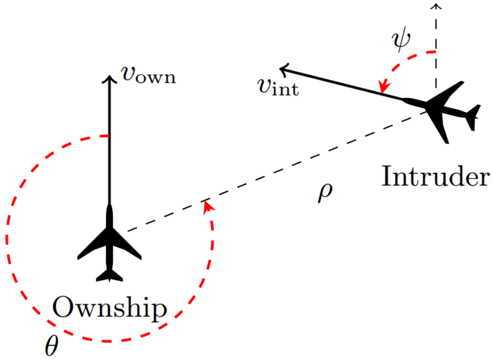
Figure 9: Vertical view of the inputs of ACAS Xu networks. [28]

The Airborne Collision Avoidance System Xu (ACAS Xu) is a mid-air collision avoidance system focusing on unmanned aircrafts. The ACAS Xu networks (ACAS Xu DNNs) provide advisories for horizontal maneuvers to avoid collisions while minimizing unnecessary alerts. The ACAS Xu benchmark consists of a set of 45 feedforward neural networks, each with seven fully connected layers, comprising a combined count of 300 neurons. Each network possesses five inputs (see Figure 9) and five outputs. For further information about the ACAS Xu benchmark see [27, 28].

For our evaluation, we first compute the reachable set of the networks. Afterward, we check whether the reachable set is fully included in the safe zone. If yes then the FNN is safe, otherwise we can conclude unsafety only for the exact analysis. We check the safety verification time (VT) in seconds, using the ten safety properties $\phi_{1},\phi_{2},\ldots,\phi_{10}$ from [28].

prop.	Exact	Overapprox.
	AVG VT(s)	AVG VT(s)
$\phi_{1}$	$\mathbf{35244.9}$	$2293.4$
$\phi_{2}$	$44\,715.5$	$2316.2$
$\phi_{3}$	$\mathbf{279.4}$	$12.4$
$\phi_{4}$	$\mathbf{98.0}$	$11.4$

Table 3: Average Verification results for properties $\phi_{1},\phi_{2},\phi_{3},\phi_{4}$ in seconds.

According to the condensed results, which are shown in Table 3, we can conclude that the star set approach is able to correctly verify the safety properties. We marked with boldface numbers, where the given property could be verified on all the relevant networks. In case of exact analysis of $\phi_{2}$, the verification results were correct, but in case of 3 networks, timeout occurred. The over-approximate analysis could verify correctly only a subset of the networks. We refer to the Appendix A.2 of this paper for the detailed results, where we show the reachability result and safety verification times of each property and network combinations. Regarding the running time of the reachability analysis: a meaningful comparison could have been made with the implementation provided in [58]; however, it is in Matlab and currently, we do not own a Matlab license.

4.2 Drone Hovering

[capbesideposition=right,center,capbesidewidth=5.425cm]table[] $ACx_{y}$ Exact Overapprox. RT(s) RES CT(s) RT(s) RES CT(s) $AC1_{1}$ $61.4$ True $4.9$ $0.2$ False $0.0$ $AC1_{2}$ $0.5$ True $0.0$ $0.1$ False $0.0$ $AC2_{1}$ $462.4$ True $17.7$ $0.5$ False $0.0$ $AC2_{2}$ $0.1$ True $0.0$ $0.1$ False $0.0$ $AC3_{1}$ - - - $2.9$ False $0.4$ $AC3_{2}$ $5.1$ True $0.1$ $0.2$ False $0.0$ $AC4_{1}$ - - - $8.7$ False $1.5$ $AC4_{2}$ $103.0$ True $5.5$ $0.7$ False $0.0$ $AC5_{1}$ $304.8$ True $26.1$ $0.4$ False $0.1$ $AC5_{2}$ $0.1$ False $0.0$ $0.1$ False $0.0$ $AC6_{1}$ $2631.7$ True $84.4$ $0.7$ False $0.1$ $AC6_{2}$ $0.1$ False $0.0$ $0.1$ False $0.0$ $AC7_{1}$ - - - $2.5$ False $0.1$ $AC7_{2}$ $4.1$ True $0.1$ $0.3$ False $0.0$ $AC8_{1}$ - - - $65.9$ False $19.8$ $AC8_{2}$ $0.8$ False $0.0$ $0.6$ False $0.0$

Table 4: Evaluation results of the drones benchmark. The network is identified as $ACx$, the lower-right index $y$ shows the tested property. RT is the reachable set computation time, and CT is the safety checking time, both in seconds. RES is the safety verification result. True indicates that the given neural network was verified to be safe, with respect to the property. Conversely, False means that the network could not be verified as safe (either because of over-approximation error or due to the network being inherently unsafe). Cells with (-) indicate cases where timeout occurs.

Autonomous drone control revolves around launching a drone into the air and enabling it to hover at a desired altitude [19, 18]. This benchmark consists of eight neural networks. The first four consist of two, and the other four networks consist of three hidden layers, each followed by a ReLU activation function. For further info about the benchmark we refer to [39]. We compute the reachability set of the networks as well as the safety verification using our algorithm and measure the reachable set computation time and safety checking time in seconds. The networks are verified both with the exact and the over-approximation method. For each neural network we test two properties. The presented results in Table 4 show, as we would expect, that the over-approximative method is much faster compared to the exact algorithm. However, the exact method verifies almost every property while the over-approximate approach fails in all cases (though some were inherently unsafe). This confirms that the over-approximate analysis is more scalable and has a smaller computational cost; however, it sacrifices the completeness of the method.

4.3 Thermostat Controller

This benchmark mentioned in the Master’s thesis [26] maintains the room temperature $x$ between $17\degree C$ and $23\degree C$ using a thermostat. It achieves this by activating (mode on) and deactivating (mode off) the heater based on the sensed temperature. The neural network representing the thermostat’s controller is a feedforward neural network with four layers. The input consists of two neurons that express the temperature $x\in\mathbb{R}$ and the current mode (on or off) as $m\in\{0,1\}$. Furthermore, two hidden layers follow, each with ten neurons. Lastly, using the unit step activation function, the output layer predicts whether the heater should turn on or off, producing the control input $Kh=15$ or $Kh=0$, respectively. We compute the reachable sets to verify the safety of the described NN using our reachability method.

We tested one safety property of the thermostat controller, the input temperature being between $22\degree$ and $23\degree$, and the thermostat being turned on, i.e., $m=1$, the expected control output should be the turn off signal. However, the reachability analysis shows two resulting star sets representing the value 15, meaning that the neural network violates its safety specification. Therefore, we take those star sets and construct the complete counter input set to falsify the neural network, i.e., prove that it is unsafe. The construction of the complete counter input set works as explained in Theorem 2 of [55].

4.4 Sonar Binary Classifier

	$\delta=0.01$		$\delta=0.001$		$\delta=0.0001$		$\delta=0.00001$
	RT	RES	RT	RES	RT	RES	RT	RES
Set 1	4359	False	783	True	263	True	102	True
Set 2	206243	False	1284	True	245	True	100	True
Set 3	33945	True	3768	True	401	True	308	True
Set 4	7974	True	359	True	103	True	102	True

Table 5: Local adversarial robustness tests of the exact approach. RT is the reachable set computation time in milliseconds. RES is the safety verification result. True indicates that the neural network correctly classifies the input set, while False means that the network was unable to correctly classify the input set.

In this section, we evaluate the robustness of a neural network used for binary classification of a sonar dataset. This dataset describes sonar chirp returns bouncing off from different objects [6]. It contains $60$ input variables representing the returned beams’ strength at different angles. The verified neural network should be capable of robust binary classification, distinguishing between rocks and metal cylinders. The neural network consists of one hidden layer with 60 neurons, followed by a ReLU activation and an output layer with a single neuron, followed by the composition of a hard sigmoid and a unit step activation function. The property we want to verify is the local robustness of the neural network. A neural network is $\delta$-locally-robust at input $x$, if for every $x^{\prime}$ such that $\left\lVert x-x^{\prime}\right\rVert_{\infty}\leq\delta$, the network assigns the same output label to $x$ and $x^{\prime}$. Our focus lies in determining the robustness threshold that our verification method can provide for the network (i.e., finding the largest $\delta$ for which the robustness property still holds).

	$\delta=0.01$		$\delta=0.001$		$\delta=0.0001$		$\delta=0.00001$
	RT	RES	RT	RES	RT	RES	RT	RES
Set 1	234	Inconclusive	205	True	163	True	103	True
Set 2	396	Inconclusive	279	True	157	True	103	True
Set 3	407	Inconclusive	367	True	177	True	174	True
Set 4	339	True	167	True	104	True	101	True

Table 6: Local adversarial robustness tests of the over-approximate approach. RT is the reachable set computation time in milliseconds. RES is the safety verification result. True indicates that the neural network correctly classifies the input set, while False means that the network was unable to correctly classify the input set. Additionally, Inconclusive is assigned when the reachability analysis algorithm cannot provide a conclusive answer due to the over-approximation errors.

We examine this problem on four inputs of the dataset and four $\delta$ values. The first two inputs should output 1, which means a rock, and the next two 0, which means a metal cylinder. The True results indicate correct classifications within the robustness threshold ($\forall x^{\prime}$ being correctly classified), False denotes incorrect predictions. Moreover, in the case of over-approximate analysis, Inconclusive means that the verification result is ambiguous due to over-approximation error. A comparison between the exact and over-approximative algorithms reveals that the exact algorithm proves network robustness in more cases. Furthermore, different input sets (meaning a single input and its $\delta$ neighborhood) exhibit varying local robustness. For example, in Table 5, for Set 2, the optimal $\delta$ value is between 0.01 and 0.001. Tables 5 and 6 are condensed versions of our experiments, to see the complete results, please check the Appendix A.3 of this paper.

5 Conclusion

In this paper, we proposed algorithms for star-based reachability analysis of various activation functions used in feed-forward neural networks. To ensure generality, we implemented the activation functions with flexibility for adaptation to specific use cases. We implemented an NNET parser in Hypro to simplify the incorporation of additional benchmarks. The presented evaluation results offer valuable insights into network behavior and safety.

As future work, we plan to integrate further layer types. Consequently, we are planning to integrate a more widely-used standard such as ONNX, for storing and parsing neural network inputs. Moreover, comprehensive experiments and evaluations will offer deeper insights into the performance, accuracy, and limitations of this analysis method when applied to neural networks with other activation functions and layer types, hence, exploring its effectiveness on a more realistic and diverse scale of benchmarks.

We also plan to integrate backpropagation methods using star-sets. Backpropagation is a widely used algorithm for training artificial neural networks, offering numerous advantages in efficient training, scalability, flexibility, and generalization capabilities [63]. Investigating the compatibility and benefits of incorporating backpropagation with star sets can significantly contribute to the advancement of safe and reliable neural networks.

Finally, we are planning to adapt abstraction refinement techniques (such as CEGAR), to reduce the over-approximation error during the reachable set analysis.

Acknowledgements. We are grateful to Dario Guidotti, Stefano Demarchi, and Armando Tacchella for generously sharing with us their drone hovering benchmark. This project has received funding from the European Union’s Horizon 2020 programme under the Skłodowska-Curie grant agreement No. 956200.

Appendix A Supplementary Material

A.1 Formal proofs

Proposition A.1 (Convex polytopes as stars).

For any $m,p\in\mathbb{N}$, $\mathbf{C}\in\mathbb{R}^{p\times m}$ and $\mathbf{d}\in\mathbb{R}^{p}$, the convex polyhedron $\mathcal{P}=\{\mathbf{x}\in\mathbb{R}^{m}\mid\mathbf{C}\mathbf{x}\leq\mathbf{d}\}$ can be represented by a star.

Proof.

It is straightforward to obtain an equivalent starset $\theta$ of the polytope $\mathcal{P}$, using the null vector as center, i.e., $\mathbf{c}=[0,0,\ldots,0]^{\intercal}$, the set of $n$ unit vectors $\mathbf{e}_{i}$ for the basis, i.e. $\mathbf{V}=\{\mathbf{e}_{1},\ldots,\mathbf{e}_{n}\}$ (i.e., the generator matrix $\mathbf{V}=\mathbb{I}_{n}$), and the predicate $P$ in the form of $\mathbf{\alpha}\in P\equiv\mathbf{C}\mathbf{\alpha}\leq\mathbf{d}$. ∎

Proposition A.2 (Affine transformation).

Assume an $(n,m)$-dimensional star $\theta=\langle{\mathbf{c},\mathbf{V},P}\rangle$ and let $\mathbf{W}\in\mathbb{R}^{k\times n}$ and $\mathbf{b}\in\mathbb{R}^{k}$. Then the affine transformation $\{\mathbf{W}\mathbf{x}+\mathbf{b}\mid\mathbf{x}\in[\theta]\}$ of $[\theta]$ is represented by $\bar{\theta}=\langle{\bar{\mathbf{c}},\bar{\mathbf{V}},P}\rangle$ with $\bar{\mathbf{c}}=\mathbf{W}\mathbf{c}+\mathbf{b}$ and $\bar{\mathbf{V}}\in\mathbb{R}^{k\times m}$ with columns $\mathbf{W}\mathbf{v}^{(1)},\ldots,\mathbf{W}\mathbf{v}^{(m)}$.

Proof.

Using the definition of the resulting star set after applying the affine transformation, we have $\bar{\theta}=\{\mathbf{y}\mid\mathbf{y}=\mathbf{W}(\mathbf{c}+\sum_{j=1}^{m}{(\mathbf{\alpha}_{j}\mathbf{v}^{(j)})})+\mathbf{b}\;\text{such}\;\text{that}\;\mathbf{\alpha}\in P\}$. That means, $\bar{\theta}$ is another star, having the center $\bar{\mathbf{c}}=\mathbf{W}\mathbf{c}+\mathbf{b}$ and generator vectors $\mathbf{V}=\{\mathbf{W}\mathbf{v}^{(1)},\mathbf{W}\mathbf{v}^{(2)},\ldots,\mathbf{W}\mathbf{v}^{(2)}\}$. Note that the predicate does not change during the computation of the affine mapping of a star. ∎

Proposition A.3 (Intersection with halfspace).

Assume an $(n,m)$-dimensional star $\theta=\langle{\mathbf{c},\mathbf{V},P}\rangle$ and a half-space $\mathcal{H}=\{\mathbf{x}\in\mathbb{R}^{n}\mid\mathbf{h}^{T}\mathbf{x}\leq g\}$ with some $\mathbf{h}\in\mathbb{R}^{n}$ and $g\in\mathbb{R}$. Then the intersetion $[\theta]\cap\mathcal{H}$ is represented by the star $\bar{\theta}=\langle{\mathbf{c},\mathbf{V},P\cap{P}^{\prime}}\rangle$ with ${P}^{\prime}=\{\mathbf{\alpha}\in\mathbb{R}^{m}\,|\,(\mathbf{h}^{T}\mathbf{V})\mathbf{\alpha}\leq g-\mathbf{h}^{T}\mathbf{c}\}$.

Proof.

The resulting star is $\bar{\theta}=\{\mathbf{x}\mid\mathbf{x}=\mathbf{c}+\sum_{j=1}^{m}{(\mathbf{\alpha}_{j}\mathbf{v}^{(j)})}\;\text{s.}\;\text{t.}\;(\mathbf{\alpha}_{1},\ldots,\mathbf{\alpha}_{m})^{T}\in P\wedge\mathbf{h}^{T}\mathbf{x}\leq g\}$. Since $\mathbf{x}=\mathbf{c}+\sum_{j=1}^{m}{(\mathbf{\alpha}_{j}\mathbf{v}^{(j)})}$, the new constraint can be written as $\mathbf{h}^{T}(\mathbf{c}+\mathbf{V}\mathbf{\alpha})\leq g$, where $\mathbf{\alpha}=[\mathbf{\alpha}_{1},\ldots,\mathbf{\alpha}_{m}]^{\intercal}$. Consequently, the new predicate is $P\cap{P}^{\prime},\;{P}^{\prime}(\mathbf{\alpha})=(\mathbf{h}^{T}\mathbf{V})\mathbf{\alpha}\leq g-\mathbf{h}^{T}\mathbf{c}$. ∎

Proposition A.4 (Emptiness checking).

A star $\theta=\langle{\mathbf{c},\mathbf{V},P}\rangle$ is empty if and only if $P$ is empty.

Proof.

It is straightforward to see that only the predicate restricts the elements of a star. In other words, if the predicte does not allow any solution (i.e., it’s empty), then the star set is empty as well. ∎

Proposition A.5 (Bounding box).

Assume an $(n,m)$-dimensional star $\theta=\langle{\mathbf{c},\mathbf{V},P}\rangle$ with $\mathbf{c}=(\mathbf{c}_{1},\ldots,\mathbf{c}_{n})^{T}$, and let $\mathbf{V}_{(i)}$ be the $i^{th}$ row of $\mathbf{V}$. Let furthermore $B=\{(x_{1},\ldots,x_{n})^{T}\in\mathbb{R}^{n}\,|\,\bigwedge_{i=1}^{n}\textit{lb}_{i}\leq x_{i}\leq\textit{ub}_{i}\}$ with $\textit{lb}_{i}=\mathbf{c}_{i}+\underset{\mathbf{\alpha}\in P}{\text{min}}\;\mathbf{V}_{(i)}\mathbf{\alpha}$ and $\textit{ub}_{i}=\mathbf{c}_{i}+\underset{\mathbf{\alpha}\in P}{\text{max}}\;\mathbf{V}_{(i)}\mathbf{\alpha}$ for $i=1,\ldots,n$. Then $[\theta]\subseteq B$.

Proof.

According to the star set’s definition $\mathbf{x}_{i}=\mathbf{c}_{i}+\sum_{j=1}^{m}{\mathbf{\alpha}_{j}\mathbf{v}^{(j)}_{i}}$. That is, if we want to find the lower (or upper) bound of $\mathbf{x}_{i}$, we have to find the solution of $\mathit{minimize}_{x\in\theta}\;\mathbf{x}_{i}$ (or $\mathit{maximize}_{x\in\theta}\;\mathbf{x}_{i}$, respecitvely). Using the definition of the star set, we get $\mathbf{c}_{i}+\mathit{minimize}_{\mathbf{\alpha}\in P=\top}\;\mathbf{V}^{(i)}\mathbf{\alpha}$ (or $\mathbf{c}_{i}+\mathit{maximize}_{\mathbf{\alpha}\in P=\top}\;\mathbf{V}^{(i)}\mathbf{\alpha}$). ∎

A.2 ACAS Xu Detailed Results

$N_{x,y}$	Exact				Overapproximation
	RT(s)	RES	CT(s)	OSS	RT(s)	RES	CT(s)	OSS
$N_{2,1}$	15837.45	False	325.53	193197	1338.12	False	43.21	1
$N_{2,2}$	36112.55	False	1174.41	472257	1005.57	False	68.81	1
$N_{2,3}$	18532.01	False	303.91	194275	962.63	False	74.02	1
$N_{2,4}$	8254.17	False	299.08	114155	1391.11	False	73.80	1
$N_{2,5}$	56241.64	False	2275.48	677510	1790.96	False	111.03	1
$N_{2,6}$	25991.47	False	650.43	309631	2044.11	False	45.39	1
$N_{2,7}$	65508.57	False	1544.92	679523	3366.64	False	161.01	1
$N_{2,8}$	53195.81	False	1260.82	585647	3677.42	False	135.44	1
$N_{2,9}$	-	-	-	-	1855.61	False	64.66	1
$N_{3,1}$	15559.97	False	727.35	252793	939.06	False	54.55	1
$N_{3,2}$	12911.84	False	295.19	181433	2362.05	False	72.16	1
$N_{3,3}$	24675.76	True	508.77	341669	900.05	False	33.53	1
$N_{3,4}$	7393.05	False	205.80	133782	1500.14	False	95.91	1
$N_{3,5}$	23852.32	False	795.67	365066	1723.58	False	67.01	1
$N_{3,6}$	70608.24	False	2823.21	1003886	2694.87	False	120.82	1
$N_{3,7}$	41256.50	False	1233.86	475299	4753.87	False	150.12	1
$N_{3,8}$	37253.31	False	754.01	472562	1304.76	False	38.45	1
$N_{3,9}$	48309.81	False	1152.44	379221	2498.83	False	54.83	1
$N_{4,1}$	66720.59	False	854.57	402853	973.59	False	74.23	1
$N_{4,2}$	85507.29	True	1130.23	484555	1139.11	False	74.50	1
$N_{4,3}$	10627.68	False	303.07	138170	1096.26	False	38.32	1
$N_{4,4}$	12923.14	False	357.63	143424	1257.89	False	77.31	1
$N_{4,5}$	75982.74	False	1223.96	457447	3312.96	False	93.14	1
$N_{4,6}$	-	-	-	-	1802.32	False	68.50	1
$N_{4,7}$	107331.18	False	2132.42	652417	781.43	False	32.85	1
$N_{4,8}$	67596.46	False	1893.68	515113	2661.60	False	186.54	1
$N_{4,9}$	-	-	-	-	13969.59	False	29.64	1
$N_{5,1}$	30332.56	False	407.09	201773	1291.09	False	60.81	1
$N_{5,2}$	43636.56	False	486.83	261011	1173.13	False	36.83	1
$N_{5,3}$	10740.98	False	191.73	125860	1072.01	False	56.17	1
$N_{5,4}$	6221.00	False	138.55	81364	1415.43	False	109.63	1
$N_{5,5}$	31217.25	False	386.70	213059	1275.20	False	61.52	1
$N_{5,6}$	97829.27	False	1149.06	622084	2196.38	False	94.40	1
$N_{5,7}$	57210.41	False	918.01	355919	2347.15	False	92.50	1
$N_{5,8}$	101123.47	False	1521.47	544813	3443.00	False	106.33	1
$N_{5,9}$	78557.70	False	1164.09	619284	3216.64	False	92.62	1

Table 7: Verification results for property $P_{2}$ on $36$ ACAS Xu networks. (RT) is the reachable set computation time, and (CT) is the safety checking time, both in seconds. (RES) is the safety verification result. (OSS) describes the number of the output star sets. The cells with (-) correspond to networks in which our algorithm was not able to compute the reachability set successfully in less than 48 hours.

$N_{x,y}$	Exact				Overapproximation
	RT(s)	RES	CT(s)	OSS	RT(s)	RES	CT(s)	OSS
$N_{1,1}$	3013.64	True	45.71	39835	823.72	False	7.97	1
$N_{1,2}$	3575.72	True	53.74	45648	2214.74	False	15.48	1
$N_{1,3}$	11037.81	True	200.90	114287	3211.44	False	16.37	1
$N_{1,4}$	13111.44	True	267.78	154529	2915.33	False	21.64	1
$N_{1,5}$	9756.54	True	196.13	122297	1618.80	False	9.97	1
$N_{1,6}$	35718.94	True	823.34	376647	1385.90	False	13.06	1
$N_{1,7}$	4712.34	True	85.86	66416	1228.45	False	13.30	1
$N_{1,8}$	8279.50	True	174.76	110139	2226.28	False	38.84	1
$N_{1,9}$	9136.22	True	189.03	135645	2999.83	False	24.42	1
$N_{2,1}$	15355.00	True	325.53	193197	1538.98	False	11.57	1
$N_{2,2}$	34071.21	True	617.56	472257	1147.34	False	19.50	1
$N_{2,3}$	13319.28	True	253.42	194275	956.66	False	18.24	1
$N_{2,4}$	8124.85	True	167.98	114155	1141.23	False	21.41	1
$N_{2,5}$	53191.97	True	1103.15	677510	1489.67	False	22.42	1
$N_{2,6}$	23772.93	True	417.89	309631	1972.41	False	10.89	1
$N_{2,7}$	53504.01	True	1016.92	679523	3330.97	False	39.63	1
$N_{2,8}$	48084.68	True	777.85	585647	4132.09	False	38.59	1
$N_{2,9}$	86837.06	True	1395.51	910575	2225.92	False	19.55	1
$N_{3,1}$	14553.80	True	497.52	252793	1130.78	False	22.86	1
$N_{3,2}$	16570.78	True	359.74	181433	2678.57	False	19.91	1
$N_{3,3}$	28386.63	True	649.15	341669	994.11	False	8.74	1
$N_{3,4}$	8765.59	True	154.49	133782	1662.63	False	23.46	1
$N_{3,5}$	28583.49	True	641.96	365066	1884.56	False	15.86	1
$N_{3,6}$	65843.71	True	1595.55	1003886	2494.56	False	28.20	1
$N_{3,7}$	47664.54	True	1094.01	475299	4453.61	False	36.35	1
$N_{3,8}$	38414.57	True	652.14	472562	1501.02	False	11.65	1
$N_{3,9}$	33949.16	True	746.01	379221	3221.20	False	17.70	1
$N_{4,1}$	35166.18	True	603.51	402853	1007.71	False	19.63	1
$N_{4,2}$	41913.56	True	748.73	484555	1322.22	False	21.65	1
$N_{4,3}$	9966.29	True	164.86	138170	1256.42	False	10.84	1
$N_{4,4}$	12343.79	True	213.54	143424	1295.82	False	20.12	1
$N_{4,5}$	39853.04	True	861.19	457447	3795.18	False	28.86	1
$N_{4,6}$	134265.70	True	2703.07	1296311	1816.04	False	18.24	1
$N_{4,7}$	61325.43	True	942.40	652417	999.71	False	10.53	1
$N_{4,8}$	32988.07	True	775.16	515113	2781.59	False	49.10	1
$N_{4,9}$	87048.69	True	1456.81	984701	14379.08	False	7.58	1
$N_{5,1}$	13215.58	True	262.90	201773	1284.01	False	14.30	1
$N_{5,2}$	17025.91	True	347.06	261011	1025.24	False	7.94	1
$N_{5,3}$	10237.07	True	219.97	125860	1089.35	False	13.62	1
$N_{5,4}$	5989.44	True	106.26	81364	1228.81	False	22.77	1
$N_{5,5}$	14346.32	True	239.07	213059	1361.83	False	17.98	1
$N_{5,6}$	102872.82	True	1120.75	622084	2093.55	False	22.16	1
$N_{5,7}$	31414.81	True	595.66	355919	2211.67	False	21.59	1
$N_{5,8}$	95265.60	True	886.15	544813	3226.16	False	24.57	1
$N_{5,9}$	95694.38	True	1002.30	619284	3546.82	False	24.30	1

Table 8: Verification results for property $P_{1}$ on $45$ ACAS Xu networks. RT is the reachable set computation time, and CT is the safety checking time, both in seconds. RES is the safety verification result. OSS describes the number of the output star sets.

$N_{x,y}$	Exact				Overapproximation
	RT(s)	RES	CT(s)	OSS	RT(s)	RES	CT(s)	OSS
$N_{1,1}$	1768.51	True	206.94	71930	33.88	False	1.45	1
$N_{1,2}$	1647.32	True	115.58	40273	34.65	False	4.28	1
$N_{1,3}$	442.65	True	29.13	12444	28.54	False	1.87	1
$N_{1,4}$	224.24	True	3.64	4346	12.95	True	0.09	1
$N_{1,5}$	246.37	True	4.09	4820	12.65	True	0.11	1
$N_{1,6}$	65.95	True	0.91	1281	3.79	True	0.03	1
$N_{2,1}$	485.40	True	17.82	16382	23.79	False	1.84	1
$N_{2,2}$	178.63	True	6.48	6924	10.60	False	1.04	1
$N_{2,3}$	316.67	True	10.55	10694	22.85	False	1.21	1
$N_{2,4}$	20.16	True	0.21	351	1.84	True	0.07	1
$N_{2,5}$	111.27	True	2.09	2466	8.17	True	0.11	1
$N_{2,6}$	13.62	True	0.12	255	3.79	True	0.03	1
$N_{2,7}$	60.04	True	0.91	1229	5.07	True	0.15	1
$N_{2,8}$	17.78	True	0.17	329	3.84	True	0.01	1
$N_{2,9}$	9.46	True	0.09	189	0.81	True	0.00	1
$N_{3,1}$	153.28	True	8.77	5999	5.19	True	0.73	1
$N_{3,2}$	2018.12	True	88.51	37541	27.15	False	1.97	1
$N_{3,3}$	390.10	True	12.46	7935	23.19	True	1.89	1
$N_{3,4}$	76.08	True	1.53	2100	29.34	False	2.27	1
$N_{3,5}$	44.62	True	1.19	1042	6.18	True	0.30	1
$N_{3,6}$	99.32	True	1.46	1868	15.38	False	1.73	1
$N_{3,7}$	4.20	True	0.04	107	1.39	True	0.01	1
$N_{3,8}$	33.03	True	0.55	669	5.84	True	0.28	1
$N_{3,9}$	42.36	True	0.82	1223	3.04	True	0.12	1
$N_{4,1}$	50.28	True	1.66	2298	4.80	False	0.90	1
$N_{4,2}$	627.65	True	19.89	18088	16.52	False	1.07	1
$N_{4,3}$	976.11	True	25.53	21237	19.26	False	1.15	1
$N_{4,4}$	34.30	True	0.39	560	2.86	True	0.06	1
$N_{4,5}$	9.23	True	0.23	361	2.41	True	0.03	1
$N_{4,6}$	107.72	True	1.86	2533	39.84	True	0.64	1
$N_{4,7}$	51.25	True	0.61	948	4.47	True	0.08	1
$N_{4,8}$	35.98	True	0.38	576	3.01	True	0.02	1
$N_{4,9}$	36.69	True	0.38	616	7.89	True	0.14	1
$N_{5,1}$	328.52	True	11.35	9556	12.10	False	0.66	1
$N_{5,2}$	61.58	True	2.10	2126	5.45	True	0.88	1
$N_{5,3}$	72.33	True	4.63	2906	10.64	True	3.13	1
$N_{5,4}$	33.32	True	0.86	765	4.98	True	0.09	1
$N_{5,5}$	44.61	True	1.02	1310	7.65	True	0.54	1
$N_{5,6}$	63.87	True	0.71	1166	10.97	True	0.56	1
$N_{5,7}$	4.93	True	0.04	88	0.81	True	0.01	1
$N_{5,8}$	134.31	True	2.11	2406	9.51	True	0.15	1
$N_{5,9}$	4.04	True	0.05	111	1.86	True	0.01	1

Table 9: Verification results for property $P_{3}$ on $45$ ACAS Xu networks. RT is the reachable set computation time, and CT is the safety checking time, both in seconds. RES is the safety verification result. OSS describes the number of the output star sets.

$N_{x,y}$	Exact				Overapproximation
	RT(s)	RES	CT(s)	OSS	RT(s)	RES	CT(s)	OSS
$N_{1,1}$	424.83	True	29.77	19142	12.57	False	4.78	1
$N_{1,2}$	366.72	True	23.35	13143	18.92	False	4.37	1
$N_{1,3}$	277.95	True	13.40	9837	22.69	False	1.40	1
$N_{1,4}$	24.99	True	1.42	1184	5.78	False	0.67	1
$N_{1,5}$	208.17	True	6.32	6608	6.67	False	0.39	1
$N_{1,6}$	117.16	True	3.32	4443	9.87	True	0.92	1
$N_{2,1}$	123.79	True	5.38	5066	12.60	False	2.10	1
$N_{2,2}$	149.75	True	6.18	4500	14.89	False	2.42	1
$N_{2,3}$	27.12	True	0.99	1087	3.62	True	0.72	1
$N_{2,4}$	22.95	True	0.51	913	8.44	True	0.06	1
$N_{2,5}$	88.98	True	2.45	3419	11.61	True	0.45	1
$N_{2,6}$	46.37	True	0.97	1462	15.22	True	0.46	1
$N_{2,7}$	18.88	True	0.29	555	5.68	True	0.08	1
$N_{2,8}$	126.04	True	1.03	1805	51.33	False	1.45	1
$N_{2,9}$	8.05	True	0.06	157	1.85	True	0.01	1
$N_{3,1}$	160.56	True	5.17	4281	9.46	True	1.15	1
$N_{3,2}$	231.23	True	14.38	8708	4.15	True	1.19	1
$N_{3,3}$	25.16	True	1.25	1201	2.44	True	0.16	1
$N_{3,4}$	31.60	True	1.22	1214	4.10	True	0.27	1
$N_{3,5}$	122.59	True	5.01	3630	26.23	True	1.13	1
$N_{3,6}$	62.39	True	1.21	1495	14.23	True	0.85	1
$N_{3,7}$	55.24	True	0.48	862	5.02	True	0.12	1
$N_{3,8}$	20.56	True	0.56	542	8.46	False	0.35	1
$N_{3,9}$	148.09	True	1.57	2684	15.36	True	0.95	1
$N_{4,1}$	19.95	True	0.87	848	1.34	True	0.35	1
$N_{4,2}$	38.94	True	1.41	1348	9.42	True	2.55	1
$N_{4,3}$	78.86	True	3.72	3725	12.85	True	4.57	1
$N_{4,4}$	58.67	True	0.82	1253	19.74	False	1.14	1
$N_{4,5}$	45.51	True	0.71	1255	8.60	True	0.23	1
$N_{4,6}$	87.67	True	1.65	2366	11.26	True	0.56	1
$N_{4,7}$	6.78	True	0.10	216	3.65	True	0.08	1
$N_{4,8}$	79.35	True	1.01	1591	9.29	True	0.09	1
$N_{4,9}$	139.12	True	1.75	2566	9.37	True	0.20	1
$N_{5,1}$	166.59	True	9.26	6932	9.45	True	0.63	1
$N_{5,2}$	117.59	True	6.30	4361	4.22	True	0.56	1
$N_{5,3}$	42.58	True	2.18	1662	7.46	True	0.71	1
$N_{5,4}$	40.08	True	1.24	1088	5.68	True	0.16	1
$N_{5,5}$	52.80	True	0.89	1549	7.65	True	0.24	1
$N_{5,6}$	27.96	True	0.50	677	6.74	True	0.47	1
$N_{5,7}$	6.08	True	0.06	157	2.63	True	0.04	1
$N_{5,8}$	24.29	True	0.28	502	12.76	True	0.73	1
$N_{5,9}$	34.99	True	0.55	992	5.26	True	0.15	1

Table 10: Verification results for property $P_{4}$ on $42$ ACAS Xu networks. RT is the reachable set computation time, and CT is the safety checking time, both in seconds. RES is the safety verification result. OSS describes the number of the output star sets.

$N_{x,y}$	Exact				Overapproximation
	RT(s)	RES	CT(s)	OSS	RT(s)	RES	CT(s)	OSS
$N_{1,1}$	2933.99	True	352.76	59734	461.70	False	8.63	1

Table 11: Verification results for property $P_{5}$ on $1$ ACAS Xu network. RT is the reachable set computation time, and CT is the safety checking time, both in seconds. RES is the safety verification result. OSS describes the number of the output star sets.

$N_{x,y}$	Exact				Overapproximation
	RT(s)	RES	CT(s)	OSS	RT(s)	RES	CT(s)	OSS
$N_{1,1}$	44026.93	True	1159.88	187775	1083.38	False	17.91	1

Table 12: Verification results for property $P_{6}$ on $1$ ACAS Xu network. RT is the reachable set computation time, and CT is the safety checking time, both in seconds. RES is the safety verification result. OSS describes the number of the output star sets.

$N_{x,y}$	Exact				Overapproximation
	RT(s)	RES	CT(s)	OSS	RT(s)	RES	CT(s)	OSS
$N_{11}$	-	-	-	-	1520.91	False	147.38	1

Table 13: Verification results for property $P_{7}$ on $1$ ACAS Xu network. RT is the reachable set computation time, and CT is the safety checking time, both in seconds. RES is the safety verification result. OSS describes the number of the output star sets. The cells with (-) correspond to networks in which our algorithm was not able to compute the reachability set successfully in less than 48 hours

$N_{x,y}$	Exact				Overapproximation
	RT(s)	RES	CT(s)	OSS	RT(s)	RES	CT(s)	OSS
$N_{2,9}$	-	-	-	-	1560.52	False	46.37	1

Table 14: Verification results for property $P_{8}$ on $1$ ACAS Xu network. RT is the reachable set computation time, and CT is the safety checking time, both in seconds. RES is the safety verification result. OSS describes the number of the output star sets. The cells with (-) correspond to networks in which our algorithm was not able to compute the reachability set successfully in less than 48 hours.

$N_{x,y}$	Exact				Overapproximation
	RT(s)	RES	CT(s)	OSS	RT(s)	RES	CT(s)	OSS
$N_{3,3}$	33727.84	False	458.09	338600	541.62	False	7.83	1

Table 15: Verification results for property $P_{9}$ on $1$ ACAS Xu network. RT is the reachable set computation time, and CT is the safety checking time, both in seconds. RES is the safety verification result. OSS describes the number of the output star sets.

$N_{x,y}$	Exact				Overapproximation
	RT(s)	RES	CT(s)	OSS	RT(s)	RES	CT(s)	OSS
$N_{4,5}$	3281.44	True	181.59	41088	1087.41	False	17.68	1

Table 16: Verification results for property $P_{10}$ on $1$ ACAS Xu network. RT is the reachable set computation time, and CT is the safety checking time, both in seconds. RES is the safety verification result. OSS describes the number of the output star sets.

A.3 Sonar Binary Classifier Detailed Results

Table 17: Local adversarial robustness tests of the exact approach. RT is the reachable set computation time in milliseconds. RES is the safety verification result. True indicates that the neural network correctly classifies the input set as expected, while False means that the neural network was unable to correctly classify the input set. Cells with (-) indicate cases where timeout occurs.

	$\delta=0.01$		$\delta=0.001$		$\delta=0.0001$		$\delta=0.00001$
	RT	RES	RT	RES	RT	RES	RT	RES
1	4359	False	783	True	263	True	102	True
2	1848	False	100	True	101	True	101	True
3	206243	False	1284	True	245	True	100	True
4	49216	False	220	False	98	True	102	True
5	253978	False	1248	True	99	True	123	True
6	6452	False	622	True	276	True	101	True
7	25640	False	98	False	99	False	103	False
8	646937	False	18313	False	448	True	101	True
9	5149	False	100	False	101	False	103	False
10	6860	False	1757	False	240	True	107	True
11	10646	False	317	True	104	True	102	True
12	2542	False	281	True	100	True	100	True
13	125001	False	418	False	101	True	101	True
14	2022	False	122	False	99	False	101	False
15	14478	False	240	False	99	False	102	False
16	17343	False	263	True	99	True	102	True
17	21727	False	250	False	97	True	101	True
18	289475	False	1066	False	98	True	101	True
19	6654	True	102	True	99	True	100	True
20	-	-	46162	False	99	True	101	True
21	53343	False	99	True	100	True	101	True
22	26779	False	192	True	100	True	104	True
23	14711	False	444	True	98	True	101	True
24	11783	True	309	True	100	True	101	True
25	3145	True	255	True	100	True	102	True
26	3529	False	99	True	104	True	101	True
27	966607	False	16329	False	476	True	194	True
28	6241	False	119	False	100	True	107	True
29	180773	False	103	True	101	True	101	True
30	96317	False	459	True	251	True	102	True
31	6667	False	111	True	100	True	103	True
32	18427	False	253	True	100	True	102	True
33	132122	True	307	True	100	True	101	True
34	478050	False	6562	False	395	True	101	True
35	35769	False	223	True	101	True	101	True
36	34491	False	1266	False	282	True	101	True
37	47224	False	101	True	106	True	102	True
38	1127	False	102	True	101	True	101	True
39	10811	False	103	True	101	True	102	True
40	15289	True	140	True	101	True	102	True
41	3926	False	690	True	103	True	101	True
42	82744	True	444	True	100	True	102	True
43	15145	True	166	True	100	True	103	True
44	2509	True	100	True	105	True	100	True
45	30090	False	117	True	99	True	100	True
46	754722	False	789	False	100	True	104	True
47	105796	False	1501	False	101	True	101	True
48	5791	False	99	False	100	False	104	False
49	19318	False	103	False	100	True	100	True
50	24453	False	217	False	101	True	100	True
51	12330	False	436	True	99	True	101	True
52	337889	True	100	True	101	True	103	True
53	4480	False	112	True	116	True	101	True
54	8742	False	100	True	102	True	101	True
55	2912	False	257	False	100	True	100	True
56	9405	False	104	False	102	True	102	True
57	15708	False	118	False	100	True	101	True
58	8188	False	163	True	100	True	104	True
59	2663	False	102	True	103	True	101	True
60	14901	False	102	True	101	True	101	True
61	1608	False	221	True	100	True	101	True
62	2251	False	179	True	104	True	101	True
63	2915	False	103	True	101	True	102	True
64	177838	True	259	True	267	True	103	True
65	3152	True	114	True	103	True	103	True
66	11178	True	102	True	103	True	102	True
67	54060	True	585	True	161	True	115	True
68	6936	False	276	True	100	True	101	True
69	6557	False	389	True	103	True	101	True
70	16761	False	306	True	183	True	188	True
71	40704	False	275	True	100	True	99	True
72	7142	False	384	True	105	True	100	True
73	97419	False	1020	False	101	True	101	True
74	8259	False	1175	False	101	True	102	True
75	118488	True	100	True	102	True	101	True
76	38638	False	246	True	100	True	100	True
77	24556	False	101	True	100	True	101	True
78	88296	False	399	False	102	True	101	True
79	67012	False	244	True	101	True	116	True
80	35943	False	388	False	161	True	100	True
81	40865	False	103	True	103	True	102	True
82	-	-	401	True	100	True	101	True
83	1435255	False	943	True	100	True	101	True
84	879783	False	2954	False	104	True	101	True
85	-	-	466010	False	286	True	101	True
86	59286	False	210	True	100	True	100	True
87	181884	False	1866	True	100	True	101	True
88	30037	False	573	True	285	True	276	True
89	79237	False	449	True	103	True	101	True
90	15188	False	193	False	100	True	100	True
91	3272	True	131	True	100	True	101	True
92	13264	False	246	False	100	True	102	True
93	30169	False	283	False	103	False	101	False
94	3518	False	1950	False	255	True	251	True
95	2507	False	99	True	100	True	102	True
96	28120	True	174	True	111	True	102	True
97	167384	True	414	True	209	True	125	True
98	33945	True	3768	True	401	True	308	True
99	7974	True	359	True	103	True	102	True
100	12175	True	4981	True	233	True	102	True
101	1486	True	100	True	101	True	102	True
102	254	True	102	True	101	True	101	True
103	1281	True	208	True	115	True	102	True
104	4265	True	167	True	101	True	102	True
105	1894	True	99	True	107	True	101	True
106	18441	True	101	True	100	True	101	True
107	50497	False	341	True	104	True	101	True
108	4747	True	1125	True	101	True	101	True
109	74918	True	101	True	100	True	102	True
110	4394	True	763	True	268	True	101	True
111	11408	True	103	True	101	True	100	True
112	9260	True	163	True	99	True	101	True
113	2292	True	99	True	100	True	99	True
114	15426	True	544	True	101	True	101	True
115	13498	True	99	True	101	True	101	True
116	28109	True	100	True	103	True	101	True
117	9277	False	219	True	102	True	101	True
118	15982	True	148	True	100	True	101	True
119	1954	True	285	True	100	True	101	True
120	1786	True	283	True	102	True	102	True
121	3574	True	505	True	286	True	102	True
122	20352	True	100	True	100	True	101	True
123	4438	True	177	True	121	True	100	True
124	6523	True	101	True	119	True	101	True
125	4662	True	286	True	101	True	100	True
126	1024	True	170	True	171	True	100	True
127	61120	True	139	True	100	True	101	True
128	2719	True	278	True	100	True	100	True
129	11209	True	150	True	101	True	100	True
130	4386	True	100	True	107	True	100	True
131	2130	True	162	True	99	True	101	True
132	10842	True	179	True	100	True	100	True
133	8829	True	100	True	101	True	101	True
134	1257	True	340	True	101	True	101	True
135	13869	True	171	True	103	True	99	True
136	1025	True	131	True	100	True	101	True
137	1991	True	235	True	99	True	101	True
138	1061	True	99	True	102	True	104	True
139	5666	True	99	True	100	True	100	True
140	1339	True	490	True	99	True	103	True
141	1115	True	98	True	99	True	100	True
142	7571	True	159	True	100	True	101	True
143	463	True	99	True	102	True	104	True
144	1871	True	262	True	100	True	100	True
145	21578	True	341	True	100	True	101	True
146	21035	True	475	True	193	True	104	True
147	572	True	98	True	99	True	100	True
148	563	True	98	True	102	True	99	True
149	36945	True	99	True	130	True	101	True
150	6400	True	100	True	109	True	100	True
151	68362	True	102	True	101	True	100	True
152	5669	True	151	True	106	True	140	True
153	17600	True	156	True	100	True	101	True
154	11486	True	103	True	102	True	99	True
155	2891	True	237	True	100	True	101	True
156	68190	True	580	True	101	True	101	True
157	10525	True	99	True	100	True	102	True
158	1928	True	98	True	99	True	101	True
159	2401	True	272	True	102	True	100	True
160	6601	True	99	True	101	True	101	True
161	1920	True	223	True	100	True	100	True
162	1038	True	273	True	115	True	101	True
163	3557	True	99	True	101	True	101	True
164	25147	True	397	True	100	True	100	True
165	11193	True	98	True	100	True	105	True
166	1910	True	99	True	101	True	100	True
167	3131	True	320	True	116	True	114	True
168	1138	True	240	True	101	True	110	True
169	1829	True	164	True	105	True	100	True
170	1653	True	170	True	101	True	100	True
171	1018	True	169	True	163	True	107	True
172	736	True	99	True	106	True	100	True
173	4313	True	99	True	105	True	101	True
174	37584	True	99	True	102	True	102	True
175	538	True	192	True	197	True	101	True
176	10231	True	343	True	157	True	153	True
177	4989	True	111	True	100	True	106	True
178	2044	True	101	True	101	True	108	True
179	649	True	101	True	105	True	101	True
180	592	True	101	True	101	True	101	True
181	332	True	100	True	99	True	101	True
182	166	True	99	True	99	True	100	True
183	382	True	99	True	100	True	101	True
184	368	True	100	True	100	True	100	True
185	515	True	191	True	100	True	100	True
186	461	True	99	True	101	True	101	True
187	808	True	164	True	99	True	100	True
188	2518	True	98	True	109	True	102	True
189	608	True	100	True	100	True	101	True
190	1162	True	99	True	99	True	100	True
191	1297	True	100	True	100	True	101	True
192	2890	True	100	True	100	True	102	True
193	2765	True	99	True	100	True	102	True
194	2336	True	164	True	102	True	102	True
195	624	True	100	True	100	True	102	True
196	1340	True	102	True	99	True	100	True
197	5056	True	258	True	100	True	101	True
198	3146	True	261	True	101	True	102	True
199	1367	True	261	True	102	True	100	True
200	2288	True	235	True	102	True	101	True
201	2449	True	201	True	101	True	102	True
202	3083	True	99	True	100	True	101	True
203	2729	True	100	True	99	True	101	True
204	2680	True	288	True	285	True	101	True
205	864	True	100	True	99	True	100	True
206	1089	True	99	True	101	True	101	True
207	866	True	101	True	99	True	103	True
208	3258	True	168	True	99	True	101	True

Table 18: Local adversarial robustness tests of the over-approximate approach. RT is the reachable set computation time in milliseconds. RES is the safety verification result. True indicates that the neural network correctly classifies the input set as expected, while False means that the neural network was unable to correctly classify the input set. Additionally, Inconclusive is assigned when the reachability analysis algorithm cannot provide a conclusive answer due to the over-approximation errors.

	$\delta=0.01$		$\delta=0.001$		$\delta=0.0001$		$\delta=0.00001$
	RT	RES	RT	RES	RT	RES	RT	RES
1	234	Inconclusive	205	True	163	True	103	True
2	278	True	103	True	102	True	103	True
3	396	Inconclusive	279	True	157	True	103	True
4	480	Inconclusive	128	True	101	True	104	True
5	391	Inconclusive	260	True	101	True	104	True
6	341	True	203	True	157	True	103	True
7	437	Inconclusive	104	False	101	False	104	False
8	403	Inconclusive	371	False	181	True	106	True
9	364	Inconclusive	102	False	101	False	103	False
10	351	Inconclusive	268	False	144	True	107	True
11	352	False	176	True	103	True	145	True
12	320	True	166	True	102	True	102	True
13	394	Inconclusive	137	False	102	True	104	True
14	289	Inconclusive	114	False	101	False	108	False
15	438	Inconclusive	214	False	101	False	102	False
16	362	False	134	True	101	True	103	True
17	321	Inconclusive	140	True	100	True	110	True
18	420	Inconclusive	193	False	100	True	104	True
19	299	True	107	True	100	True	102	True
20	454	Inconclusive	390	True	100	True	106	True
21	459	Inconclusive	105	True	101	True	103	True
22	498	True	143	True	101	True	103	True
23	369	Inconclusive	204	True	101	True	107	True
24	385	True	160	True	101	True	103	True
25	342	True	154	True	103	True	104	True
26	310	Inconclusive	101	True	103	True	105	True
27	554	Inconclusive	384	True	172	True	137	True
28	338	Inconclusive	112	True	102	True	103	True
29	564	Inconclusive	106	True	106	True	106	True
30	494	Inconclusive	167	True	158	True	104	True
31	296	Inconclusive	106	True	101	True	103	True
32	336	Inconclusive	164	True	106	True	107	True
33	512	True	156	True	102	True	104	True
34	474	Inconclusive	292	False	199	True	103	True
35	377	Inconclusive	140	True	102	True	104	True
36	436	Inconclusive	246	True	180	True	103	True
37	380	True	102	True	103	True	107	True
38	211	Inconclusive	104	True	103	True	106	True
39	436	True	101	True	111	True	104	True
40	345	True	105	True	103	True	104	True
41	321	Inconclusive	175	True	102	True	105	True
42	424	True	191	True	106	True	104	True
43	374	True	118	True	102	True	103	True
44	247	True	103	True	102	True	106	True
45	504	Inconclusive	108	True	108	True	113	True
46	574	Inconclusive	186	True	102	True	104	True
47	410	Inconclusive	253	False	102	True	106	True
48	379	Inconclusive	105	False	105	False	102	False
49	411	Inconclusive	105	False	103	True	104	True
50	396	Inconclusive	140	True	101	True	106	True
51	415	True	198	True	104	True	102	True
52	497	True	106	True	103	True	103	True
53	346	Inconclusive	111	True	106	True	111	True
54	339	Inconclusive	107	True	103	True	103	True
55	350	Inconclusive	145	False	102	True	104	True
56	321	Inconclusive	102	False	103	True	107	True
57	361	Inconclusive	105	True	107	True	103	True
58	323	True	120	True	102	True	103	True
59	329	False	102	True	103	True	106	True
60	443	True	102	True	104	True	103	True
61	298	False	143	True	102	True	103	True
62	431	False	128	True	104	True	107	True
63	442	False	103	True	110	True	104	True
64	434	True	153	True	156	True	104	True
65	337	True	107	True	104	True	105	True
66	402	True	103	True	103	True	119	True
67	441	True	207	True	131	True	104	True
68	425	False	157	True	109	True	102	True
69	378	False	181	True	102	True	126	True
70	426	Inconclusive	155	True	133	True	147	True
71	418	Inconclusive	164	True	105	True	103	True
72	416	Inconclusive	180	True	104	True	103	True
73	447	Inconclusive	203	False	104	True	105	True
74	298	Inconclusive	218	False	103	True	104	True
75	507	True	103	True	104	True	103	True
76	479	Inconclusive	145	True	105	True	103	True
77	502	Inconclusive	105	True	104	True	104	True
78	476	Inconclusive	176	True	105	True	102	True
79	505	Inconclusive	144	True	107	True	102	True
80	389	Inconclusive	186	True	128	True	103	True
81	495	Inconclusive	103	True	102	True	103	True
82	569	Inconclusive	176	True	102	True	104	True
83	541	Inconclusive	251	True	104	True	103	True
84	515	Inconclusive	337	True	104	True	104	True
85	578	Inconclusive	413	False	158	True	103	True
86	349	Inconclusive	130	True	103	True	103	True
87	414	False	251	True	104	True	103	True
88	367	Inconclusive	202	True	158	True	171	True
89	427	Inconclusive	161	True	102	True	102	True
90	326	Inconclusive	126	False	102	True	104	True
91	259	True	110	True	105	True	103	True
92	436	Inconclusive	150	True	103	True	104	True
93	410	Inconclusive	152	True	103	False	104	False
94	293	Inconclusive	208	True	147	True	146	True
95	286	Inconclusive	103	True	103	True	102	True
96	411	True	126	True	114	True	105	True
97	586	True	139	True	128	True	112	True
98	407	Inconclusive	367	True	177	True	174	True
99	339	True	167	True	104	True	101	True
100	405	Inconclusive	301	True	145	True	104	True
101	259	True	103	True	110	True	104	True
102	141	Inconclusive	106	True	107	True	103	True
103	359	True	142	True	101	True	103	True
104	317	True	127	True	104	True	105	True
105	313	True	101	True	108	True	103	True
106	329	Inconclusive	101	True	103	True	102	True
107	503	Inconclusive	151	True	101	True	104	True
108	342	Inconclusive	229	True	108	True	103	True
109	401	Inconclusive	102	True	102	True	103	True
110	383	Inconclusive	225	True	156	True	103	True
111	366	Inconclusive	102	True	141	True	102	True
112	299	True	119	True	129	True	102	True
113	305	Inconclusive	102	True	103	True	103	True
114	379	Inconclusive	190	True	104	True	105	True
115	378	Inconclusive	101	True	103	True	103	True
116	413	Inconclusive	102	True	103	True	104	True
117	377	Inconclusive	136	True	107	True	103	True
118	361	True	116	True	103	True	103	True
119	293	Inconclusive	159	True	103	True	105	True
120	260	True	149	True	109	True	103	True
121	320	Inconclusive	218	True	185	True	104	True
122	398	True	101	True	105	True	103	True
123	328	True	127	True	103	True	103	True
124	360	Inconclusive	102	True	102	True	103	True
125	328	True	165	True	103	True	103	True
126	251	Inconclusive	125	True	131	True	103	True
127	354	True	113	True	104	True	103	True
128	331	Inconclusive	150	True	108	True	104	True
129	264	True	120	True	103	True	102	True
130	314	True	102	True	102	True	102	True
131	233	True	126	True	138	True	103	True
132	285	True	123	True	101	True	103	True
133	359	True	103	True	106	True	104	True
134	185	True	157	True	105	True	103	True
135	403	True	126	True	105	True	102	True
136	260	True	112	True	103	True	102	True
137	232	True	144	True	103	True	105	True
138	226	True	102	True	102	True	103	True
139	380	True	101	True	104	True	102	True
140	256	True	232	True	102	True	103	True
141	293	True	101	True	107	True	105	True
142	352	True	118	True	101	True	102	True
143	197	True	101	True	104	True	104	True
144	296	True	158	True	104	True	102	True
145	359	True	149	True	103	True	102	True
146	374	True	182	True	145	True	103	True
147	195	True	100	True	103	True	106	True
148	192	True	101	True	104	True	101	True
149	484	True	102	True	134	True	102	True
150	376	True	102	True	109	True	105	True
151	564	Inconclusive	102	True	103	True	103	True
152	375	Inconclusive	116	True	103	True	138	True
153	407	Inconclusive	120	True	110	True	122	True
154	369	Inconclusive	101	True	104	True	102	True
155	303	Inconclusive	149	True	107	True	111	True
156	528	Inconclusive	196	True	103	True	104	True
157	355	True	100	True	103	True	102	True
158	315	True	102	True	102	True	104	True
159	302	True	141	True	103	True	104	True
160	304	Inconclusive	101	True	105	True	104	True
161	353	True	136	True	103	True	102	True
162	224	True	151	True	104	True	101	True
163	351	True	101	True	137	True	103	True
164	446	Inconclusive	155	True	102	True	103	True
165	401	True	100	True	105	True	103	True
166	276	Inconclusive	101	True	103	True	104	True
167	336	True	175	True	110	True	108	True
168	253	Inconclusive	159	True	104	True	102	True
169	281	Inconclusive	120	True	102	True	110	True
170	282	True	123	True	109	True	102	True
171	227	Inconclusive	125	True	122	True	102	True
172	224	True	101	True	101	True	106	True
173	323	True	101	True	116	True	103	True
174	385	True	102	True	109	True	102	True
175	213	True	138	True	137	True	104	True
176	278	True	156	True	118	True	120	True
177	324	True	105	True	101	True	103	True
178	284	Inconclusive	101	True	104	True	103	True
179	193	Inconclusive	103	True	104	True	105	True
180	227	True	101	True	102	True	103	True
181	189	True	102	True	102	True	104	True
182	124	True	100	True	102	True	102	True
183	171	True	101	True	102	True	102	True
184	170	True	102	True	102	True	103	True
185	190	True	130	True	103	True	102	True
186	194	True	101	True	105	True	102	True
187	248	True	127	True	102	True	105	True
188	348	True	101	True	101	True	104	True
189	221	True	102	True	103	True	103	True
190	240	Inconclusive	102	True	102	True	103	True
191	246	True	102	True	102	True	103	True
192	293	Inconclusive	104	True	105	True	104	True
193	357	True	102	True	103	True	105	True
194	261	Inconclusive	121	True	103	True	103	True
195	208	Inconclusive	101	True	104	True	103	True
196	248	True	103	True	102	True	102	True
197	351	True	175	True	103	True	103	True
198	297	True	142	True	105	True	102	True
199	245	True	149	True	105	True	104	True
200	283	True	154	True	104	True	103	True
201	275	True	144	True	108	True	102	True
202	280	True	102	True	102	True	106	True
203	323	True	102	True	102	True	102	True
204	274	True	165	True	177	True	103	True
205	247	True	101	True	102	True	105	True
206	250	True	102	True	103	True	103	True
207	236	True	101	True	101	True	104	True
208	302	Inconclusive	129	True	101	True	102	True

References

- [1]
- [2] Oludare Isaac Abiodun, Aman Jantan, Abiodun Esther Omolara, Kemi Victoria Dada, Abubakar Malah Umar, Okafor Uchenwa Linus, Humaira Arshad, Abdullahi Aminu Kazaure, Usman Gana & Muhammad Ubale Kiru (2019): Comprehensive review of artificial neural network applications to pattern recognition. IEEE Access 7, pp. 158820–158846, 10.1109/ACCESS.2019.2945545.
- [3] Sushma Priya Anthadupula & Manasi Gyanchandani (2021): A Review and Performance Analysis of Non-Linear Activation Functions in Deep Neural Networks. Int. Res. J. Mod. Eng. Technol. Sci, 10.1109/iscid.2009.214.
- [4] Stanley Bak & Parasara Sridhar Duggirala (2017): Simulation-Equivalent Reachability of Large Linear Systems with Inputs. In Rupak Majumdar & Viktor Kunčak, editors: Computer Aided Verification, pp. 401–420, 10.1007/978-3-319-63387-9_20.
- [5] Akhilan Boopathy, Tsui-Wei Weng, Pin-Yu Chen, Sijia Liu & Luca Daniel (2019): CNN-Cert: An Efficient Framework for Certifying Robustness of Convolutional Neural Networks. Proceedings of the AAAI Conference on Artificial Intelligence 33(01), pp. 3240–3247, 10.1609/aaai.v33i01.33013240. Available at https://ojs.aaai.org/index.php/AAAI/article/view/4193.
- [6] Jason Brownlee (2022): Binary Classification Tutorial with the Keras Deep Learning Library. https://machinelearningmastery.com/binary-classification-tutorial-with-the-keras-deep-learning-library/. [Accessed : June 1, 2023].
- [7] Chih-Hong Cheng, Georg Nührenberg & Harald Ruess (2017): Maximum resilience of artificial neural networks. In: Automated Technology for Verification and Analysis: 15th International Symposium, ATVA 2017, Pune, India, October 3–6, 2017, Proceedings 15, Springer, pp. 251–268, 10.1007/978-3-319-68167-2_18.
- [8] Edmund M Clarke & Jeannette M Wing (1996): Formal methods: State of the art and future directions. ACM Computing Surveys (CSUR) 28(4), pp. 626–643, 10.1145/242223.242257.
- [9] Ronan Collobert (2004): Large scale machine learning. Technical Report, Université de Paris VI.
- [10] Ekin Cubuk, Barret Zoph, Samuel Schoenholz & Quoc Le (2017): Intriguing Properties of Adversarial Examples.
- [11] Leonid Datta (2020): A Survey on Activation Functions and their relation with Xavier and He Normal Initialization.
- [12] Educative (2023): What is the vanishing gradient problem? https://www.educative.io/answers/what-is-the-vanishing-gradient-problem. [Accessed: May 12, 2023].
- [13] Ruediger Ehlers (2017): Formal verification of piece-wise linear feed-forward neural networks. In: Automated Technology for Verification and Analysis: 15th International Symposium, ATVA 2017, Pune, India, October 3–6, 2017, Proceedings 15, Springer, pp. 269–286, 10.1007/978-3-319-68167-2_19.
- [14] Dumitru Erhan, Christian Szegedy, Alexander Toshev & Dragomir Anguelov (2014): Scalable Object Detection Using Deep Neural Networks. In: 2014 IEEE Conference on Computer Vision and Pattern Recognition, pp. 2155–2162, 10.1109/CVPR.2014.276.
- [15] Aymeric Fromherz, Klas Leino, Matt Fredrikson, Bryan Parno & Corina Pasareanu (2021): Fast Geometric Projections for Local Robustness Certification. In: International Conference on Learning Representations. Available at https://openreview.net/forum?id=zWy1uxjDdZJ.
- [16] Osvaldo Gervasi, Beniamino Murgante, Antonio Laganà, David Taniar, Youngsong Mun & Marina L. Gavrilova, editors (2008): Computational Science and Its Applications - ICCSA 2008, International Conference, Perugia, Italy, June 30 - July 3, 2008, Proceedings, Part I. Lecture Notes in Computer Science 5072, Springer, 10.1007/978-3-540-69839-5.
- [17] Ian J. Goodfellow, Jonathon Shlens & Christian Szegedy (2014): Explaining and Harnessing Adversarial Examples. CoRR abs/1412.6572. Available at https://api.semanticscholar.org/CorpusID:6706414.
- [18] Dario Guidotti (2022): Verification of Neural Networks for Safety and Security-critical Domains. ISSN 1613-0073 CEUR Workshop Proceedings. Available at https://ceur-ws.org/Vol-3345/paper10_RiCeRCa3.pdf.
- [19] Dario Guidotti, Stefano Demarchi, Luca Pulina & Armando Tacchella (2022): Evaluating Reachability Algorithms for Neural Networks on NeVer2.
- [20] Patrick Henriksen & Alessio Lomuscio (2021): DEEPSPLIT: An Efficient Splitting Method for Neural Network Verification via Indirect Effect Analysis. In: IJCAI, pp. 2549–2555, 10.24963/ijcai.2021/351.
- [21] Michael Hinchey, Jonathan Bowen & Christopher Rouff (2006): Introduction to Formal Methods. Springer, 10.1007/1-84628-271-3_2.
- [22] Geoffrey Hinton, Li Deng, Dong Yu, George E. Dahl, Abdel-rahman Mohamed, Navdeep Jaitly, Andrew Senior, Vincent Vanhoucke, Patrick Nguyen, Tara N. Sainath & Brian Kingsbury (2012): Deep Neural Networks for Acoustic Modeling in Speech Recognition: The Shared Views of Four Research Groups. IEEE Signal Processing Magazine 29(6), pp. 82–97, 10.1109/MSP.2012.2205597.
- [23] Geoffrey Hinton, Li Deng, Dong Yu, George E Dahl, Abdel-rahman Mohamed, Navdeep Jaitly, Andrew Senior, Vincent Vanhoucke, Patrick Nguyen, Tara N Sainath et al. (2012): Deep neural networks for acoustic modeling in speech recognition: The shared views of four research groups. IEEE Signal processing magazine 29(6), pp. 82–97, 10.1109/MSP.2012.2205597.
- [24] Chao Huang, Jiameng Fan, Wenchao Li, Xin Chen & Qi Zhu (2019): Reachnn: Reachability analysis of neural-network controlled systems. ACM Transactions on Embedded Computing Systems (TECS) 18(5s), pp. 1–22, 10.1145/3358228.
- [25] Xiaowei Huang, Marta Kwiatkowska, Sen Wang & Min Wu (2017): Safety verification of deep neural networks. In: International conference on computer aided verification, Springer, pp. 3–29, 10.1007/978-3-319-63387-9_1.
- [26] Ruoran Gabriela Jiang (2023): Verifying ai-controlled hybrid systems. Master’s thesis, RWTH Aachen University, Aachen, Germany. Available at https://ths.rwth-aachen.de/wp-content/uploads/sites/4/master_thesis_jiang.pdf.
- [27] Kyle D. Julian, Mykel J. Kochenderfer & Michael P. Owen (2019): Deep Neural Network Compression for Aircraft Collision Avoidance Systems. Journal of Guidance, Control, and Dynamics 42(3), pp. 598–608, 10.2514/1.g003724. Available at https://doi.org/10.2514%2F1.g003724.
- [28] Guy Katz, Clark Barrett, David L. Dill, Kyle Julian & Mykel J. Kochenderfer (2017): Reluplex: An Efficient SMT Solver for Verifying Deep Neural Networks. In Rupak Majumdar & Viktor Kunčak, editors: Computer Aided Verification, Springer International Publishing, Cham, pp. 97–117, 10.1007/978-3-319-63387-9_5.
- [29] Guy Katz, Derek A Huang, Duligur Ibeling, Kyle Julian, Christopher Lazarus, Rachel Lim, Parth Shah, Shantanu Thakoor, Haoze Wu, Aleksandar Zeljić et al. (2019): The marabou framework for verification and analysis of deep neural networks. In: International Conference on Computer Aided Verification, Springer, pp. 443–452, 10.1007/978-3-030-25540-4_26.
- [30] Philipp Kern, Marko Kleine Büning & Carsten Sinz (2022): Optimized Symbolic Interval Propagation for Neural Network Verification. In: 1st Workshop on Formal Verification of Machine Learning (WFVML 2022) colocated with ICML 2022: International Conference on Machine Learning.
- [31] Kumar, Niranjan (2019): Deep Learning: Feedforward Neural Networks Explained. https://medium.com/hackernoon/deep-learning-feedforward-neural-networks-explained- c34ae3f084f1. [Accessed: May 03, 2023].
- [32] Sampo Kuutti, Richard Bowden, Yaochu Jin, Phil Barber & Saber Fallah (2021): A Survey of Deep Learning Applications to Autonomous Vehicle Control. IEEE Transactions on Intelligent Transportation Systems 22(2), pp. 712–733, 10.1109/TITS.2019.2962338.
- [33] Yann LeCun, Yoshua Bengio & Geoffrey Hinton (2015): Deep learning. nature 521(7553), pp. 436–444, 10.1038/nature14539.
- [34] Andy Lee (2015): Comparing deep neural networks and traditional vision algorithms in mobile robotics. Swarthmore University. Available at https://api.semanticscholar.org/CorpusID:10011895.
- [35] Changliu Liu, Tomer Arnon, Christopher Lazarus, Christopher Strong, Clark Barrett & Mykel J. Kochenderfer (2021): Algorithms for Verifying Deep Neural Networks. Foundations and Trends in Optimization 4(3-4), pp. 244–404, 10.1561/2400000035. Available at http://theory.stanford.edu/~barrett/pubs/LAL+21.pdf.
- [36] Weibo Liu, Zidong Wang, Xiaohui Liu, Nianyin Zeng, Yurong Liu & Fuad E. Alsaadi (2017): A survey of deep neural network architectures and their applications. Neurocomputing 234, pp. 11–26, 10.1016/j.neucom.2016.12.038. Available at https://www.sciencedirect.com/science/article/pii/S0925231216315533.
- [37] Alessio Lomuscio & Lalit Maganti (2017): An approach to reachability analysis for feed-forward ReLU neural networks.
- [38] Andrew L. Maas (2013): Rectifier Nonlinearities Improve Neural Network Acoustic Models. In: Proceedings of the International Conference on Machine Learning, pp. 1–6. Available at https://www.semanticscholar.org/paper/Rectifier-Nonlinearities-Improve-Neural-Network-Maas/367f2c63a6f6a10b3b64b8729d601e69337ee3cc.
- [39] Hana Masara (2023): Star Set-based Reachability Analysis of Neural Networks with Differing Layers and Activation Functions. Bachelor’s thesis, RWTH Aachen University, Aachen, Germany. Available at https://ths.rwth-aachen.de/wp-content/uploads/sites/4/Thesis-Hana-Masara.pdf.
- [40] ONNX. https://onnx.ai/. [Accessed: May 30, 2023].
- [41] (2021): PyTorch: torch.nn.Hardsigmoid. https://pytorch.org/docs/stable/generated/torch.nn.Hardsigmoid.html. Accessed : May 16, 2023.
- [42] Luca Pulina & Armando Tacchella (2010): An Abstraction-Refinement Approach to Verification of Artificial Neural Networks. In Tayssir Touili, Byron Cook & Paul Jackson, editors: Computer Aided Verification, Springer Berlin Heidelberg, Berlin, Heidelberg, pp. 243–257, 10.1007/978-3-642-14295-6_24.
- [43] Luthfi Ramadhan (2021): Neural Network: The Dead Neuron. https://towardsdatascience.com/neural-network-the-dead-neuron-eaa92e575748. [Accessed: May 14, 2023].
- [44] Waseem Rawat & Zenghui Wang (2017): Deep convolutional neural networks for image classification: A comprehensive review. Neural computation 29(9), pp. 2352–2449, 10.1162/neco_a_00990.
- [45] Wenjie Ruan, Xiaowei Huang & Marta Kwiatkowska (2018): Reachability Analysis of Deep Neural Networks with Provable Guarantees. In: Proceedings of the Twenty-Seventh International Joint Conference on Artificial Intelligence, IJCAI-18, International Joint Conferences on Artificial Intelligence Organization, pp. 2651–2659, 10.24963/ijcai.2018/368. Available at https://doi.org/10.24963/ijcai.2018/368.
- [46] Wojciech Samek, Grégoire Montavon, Sebastian Lapuschkin, Christopher J Anders & Klaus-Robert Müller (2021): Explaining deep neural networks and beyond: A review of methods and applications. Proceedings of the IEEE 109(3), pp. 247–278, 10.1109/JPROC.2021.3060483.
- [47] Stefan Schupp, Erika Ábrahám, Ibtissem Makhlouf & Stefan Kowalewski (2017): HyPro: A C++ Library of State Set Representations for Hybrid Systems Reachability Analysis. In Clark Barrett, Misty Davies & Temesghen Kahsai, editors: NASA Formal Methods, pp. 288–294, 10.1007/978-3-319-57288-8_20.
- [48] Stefan Schupp, Erika Ábrahám, Ibtissem Ben Makhlouf & Stefan Kowalewski (2017): H y P ro: A C++ library of state set representations for hybrid systems reachability analysis. In: NASA Formal Methods Symposium, Springer, pp. 288–294, 10.1007/978-3-319-57288-8_20.
- [49] Stefan Schupp, Goran Frehse & Erika Ábrahám (2019): State set representations and their usage in the reachability analysis of hybrid systems. Ph.D. thesis, RWTH Aachen University, 10.18154/RWTH-2019-08875. Available at https://publications.rwth-aachen.de/record/767529/files/767529.pdf.
- [50] Gagandeep Singh, Timon Gehr, Markus Püschel & Martin T. Vechev (2019): An abstract domain for certifying neural networks. Proc. ACM Program. Lang. 3(POPL), pp. 41:1–41:30, 10.1145/3290354. Available at https://doi.org/10.1145/3290354.
- [51] Bing Sun, Jun Sun, Ting Dai & Lijun Zhang (2021): Probabilistic Verification of Neural Networks Against Group Fairness. In: Formal Methods: 24th International Symposium, FM 2021, Virtual Event, November 20-26, 2021, Proceedings, Springer-Verlag, Berlin, Heidelberg, pp. 83–102, 10.1007/978-3-030-90870-6_5. Available at https://doi.org/10.1007/978-3-030-90870-6_5.
- [52] Daniel Svozil, Vladimir Kvasnicka & Jiri Pospichal (1997): Introduction to multi-layer feed-forward neural networks. Chemometrics and Intelligent Laboratory Systems 39(1), pp. 43–62, 10.1016/S0169-7439(97)00061-0.
- [53] (2023): TensorFlow Documentation. https://www.tensorflow.org/api_docs/python/tf/keras/activations/hard_sigmoid. Accessed : May 16, 2023.
- [54] Dung Tran (2020): Verification of Learning-enabled Cyber-Physical Systems. Ph.D. thesis, Vanderbilt University Graduate School. Available at http://hdl.handle.net/1803/15957.
- [55] Hoang-Dung Tran, Diago Manzanas Lopez, Patrick Musau, Xiaodong Yang, Luan Viet Nguyen, Weiming Xiang & Taylor T. Johnson (2019): Star-Based Reachability Analysis of Deep Neural Networks. In Maurice H. ter Beek, Annabelle McIver & José N. Oliveira, editors: Formal Methods – The Next 30 Years, Springer International Publishing, Cham, pp. 670–686, 10.1007/978-3-030-30942-8_39.
- [56] Hoang-Dung Tran, Patrick Musau, Diego Manzanas Lopez, Xiaodong Yang, Luan Viet Nguyen, Weiming Xiang & Taylor T Johnson (2019): Parallelizable reachability analysis algorithms for feed-forward neural networks. In: 2019 IEEE/ACM 7th International Conference on Formal Methods in Software Engineering (FormaliSE), IEEE, pp. 51–60, 10.1109/FormaliSE.2019.00012.
- [57] Hoang-Dung Tran, Neelanjana Pal, Diego Manzanas Lopez, Patrick Musau, Xiaodong Yang, Luan Viet Nguyen, Weiming Xiang, Stanley Bak & Taylor T Johnson (2021): Verification of piecewise deep neural networks: a star set approach with zonotope pre-filter. Formal Aspects of Computing 33, pp. 519–545, 10.1007/s00165-021-00553-4.
- [58] Hoang-Dung Tran, Neelanjana Pal, Diego Manzanas Lopez, Patrick Musau, Xiaodong Yang, Luan Viet Nguyen, Weiming Xiang, Stanley Bak & Taylor T. Johnson (2021): Verification of piecewise deep neural networks: a star set approach with zonotope pre-filter. Formal Aspects of Computing 33(4), pp. 519–545, 10.1007/s00165-021-00553-4. Available at https://doi.org/10.1007/s00165-021-00553-4.
- [59] RWTH University (2023): RWTH High Performance Computing (Linux). https://help.itc.rwth-aachen.de/service/rhr4fjjutttf/. [Accessed : July 24, 2023].
- [60] Shiqi Wang, Kexin Pei, Justin Whitehouse, Junfeng Yang & Suman Jana (2018): Efficient Formal Safety Analysis of Neural Networks. In: Proceedings of the 32nd International Conference on Neural Information Processing Systems, NIPS’18, Curran Associates Inc., Red Hook, NY, USA, pp. 6369–6379.
- [61] Jeannette M Wing (1990): A specifier’s introduction to formal methods. Computer 23(9), pp. 8–22, 10.1109/2.58215.
- [62] Jim Woodcock, Peter Gorm Larsen, Juan Bicarregui & John Fitzgerald (2009): Formal methods: Practice and experience. ACM computing surveys (CSUR) 41(4), pp. 1–36, 10.1145/1592434.1592436.
- [63] Logan G. Wright, Tatsuhiro Onodera, Martin M. Stein, Tianyu Wang, Darren T. Schachter, Zoey Hu & Peter L. McMahon (2022): Deep physical neural networks trained with backpropagation. Nature 601(7894), pp. 549–555, 10.1038/s41586-021-04223-6. Available at https://doi.org/10.1038/s41586-021-04223-6.
- [64] Haoze Wu, Aleksandar Zeljić, Guy Katz & Clark Barrett (2022): Efficient Neural Network Analysis with Sum-of-Infeasibilities. In Dana Fisman & Grigore Rosu, editors: Tools and Algorithms for the Construction and Analysis of Systems, Springer International Publishing, Cham, pp. 143–163, 10.1007/978-3-030-99524-9_8.
- [65] Weiming Xiang, Hoang-Dung Tran & Taylor T. Johnson (2018): Output Reachable Set Estimation and Verification for Multilayer Neural Networks. IEEE Transactions on Neural Networks and Learning Systems 29(11), pp. 5777–5783, 10.1109/TNNLS.2018.2808470.
- [66] Jin Xu, Zishan Li, Bowen Du, Miaomiao Zhang & Jing Liu (2020): Reluplex made more practical: Leaky ReLU. In: 2020 IEEE Symposium on Computers and Communications (ISCC), pp. 1–7, 10.1109/ISCC50000.2020.9219587.