A Bayesian Inverse Approach to Proton Therapy Dose Delivery Verification

Abstract.

This study presents a proof-of-concept for a novel Bayesian inverse method in a one-dimensional setting, aimed at proton beam therapy treatment verification. Our methodology is predicated on a hypothetical scenario wherein strategically positioned sensors detect prompt-$\gamma$’s emitted from a proton beam when it interacts with defined layers of tissue. Using this data, we employ a Bayesian framework to estimate the proton beam’s energy deposition profile. We validate our Bayesian inverse estimations against a closed-form approximation of the Bragg Peak in a uniform medium and a layered lung tumour.

1. Introduction

Proton Beam Therapy (PBT) is a promising treatment for certain challenging cancers. This includes cases where conventional radiotherapy cannot adequately limit irradiation to surrounding critical tissues. Examples are pediatric cancers, cancers at the base of the skull, and complex head and neck cancers.

A proton deposits energy as it travels through matter. This energy deposition increases as the proton slows down, reaching its maximum at the end of its path, as illustrated in Figure 1.

Figure 1. An illustration of dose profiles of different radiation modalities. Notice that the dose deposition of photons is highest near the source with a decaying profile as depth increases. Protons and carbon ions are very localised with the decay of protons dropping to zero quickly after peak deposition is attained. This enables the construction of a Spread Out Bragg Peak over a target region by forming appropriate linear combinations of different energy and intensity beams. Carbon ions have an even sharper peak and dose profile upon entry but the deposition does not decay to zero after the peak due to secondary interactions.

This energy, or dose, delivers the cancer-killing effect, but can also harm surrounding healthy tissue. The objective of PBT is to administer the intended dose to the tumor, as predetermined by prior clinical evidence, while minimising exposure to the adjacent tissues. PBT’s potential for delivering a superior dose profile compared to traditional photon treatments has long been recognised [1]. A significant number of patients have received PBT treatment ([2] estimates over 275,000 worldwide as of December 2021). Nevertheless, there remains a lack of conclusive evidence regarding PBT’s benefits over conventional photon-based treatments, such as X-rays (see, for instance, [3]). As a relatively new treatment modality, fundamental challenges persist in PBT’s treatment planning and verification, limiting its broader adoption. Day-to-day variations in patient anatomy, such as those caused by water retention, introduce uncertainties. Current strategies address these uncertainties during planning either by expanding the irradiated volume - which diminishes PBT’s potential for sparing healthy tissue - or by compromising tumour coverage to ensure protection of critical surrounding tissues.

In conventional photon radiotherapy, the dose delivery location can be inferred by measuring the X-rays that exit the patient. However, while proton therapy offers superior dose delivery, verifying its precise administration is more challenging since most of the radiation dose, including the proton beam itself, remains inside the patient. This challenge, stemming from clinical need, is the focus of our investigation, and in this work we propose a flexible mathematical methodology which can form the basis for addressing this.

When protons impact tissue, the primary mechanism of energy loss involves inelastic interactions with atomic electrons. As the proton interacts with electrons, it leaves behind a trail of excitations and ionisations. There is a continual energy decrement of the proton within the tissue, which is quantified by the stopping power. Elastic interactions cause the treatment field to scatter within the tissue; interestingly, this scattering increases with depth. Non-elastic nuclear collisions can generate neutrons and other protons as secondary interactions. An additional possible result of a nuclear reaction is the decay of an unstable nucleus, which emits gamma rays, or prompt gammas (prompt-$\gamma$’s). These are termed ’prompt’ because they emerge shortly after the initial proton interaction, as shown in Figure 2.

Figure 2. The three main interactions of a proton with matter. A nonelastic proton-nucleus collision, an inelastic Coulomb interaction with atomic electrons and elastic Coulomb scattering with the nucleus.

The prompt-$\gamma$’s have energies in the range of approximately 2-10MeV. This is significantly higher than the photon energies typically employed in diagnostic imaging. As a result, there are currently no cameras specifically optimised for measuring prompt-$\gamma$’s in a clinical setting.

The aim and novelty of this work lie in introducing a Bayesian approach to explore the potential for dose delivery verification by measuring the prompt-$\gamma$ radiation emitted from the patient. The location of these emitted particles depends on the intricate interplay of the environment they traverse, which often remains not fully understood during treatment, given the limitations of tools like CT scans used for planning. Consequently, determining whether the radiation measured during the treatment aligns with the intended dose delivery poses a complex inverse problem.

Our presentation revolves around the energy dynamics during proton treatment. At the heart of our methodology is the Bortfield model [4, 5], which we use to model forward behaviour of a hypothetical scenario. We employ a Bayesian framework to ascertain the potential success of treatments using observed radiation profiles. In formulating the model we make some fundamental assumptions. We suggest that the depth of energy deposition correlates directly to the likelihood of a $\gamma$ particle’s emission. Moreover, we consider our observational data to be independent, identically distributed, and consistent over time.

A key aspect of our treatment is the data integration step. We adopt a Bayesian approach, incorporating potentially highly uncertain beliefs about the configuration of the patient, and synthesising this information though our forward modelling to determine likely configurations given the observed prompt-$\gamma$ emissions. Our approach takes the form of a Bayesian Inverse Problem, which we propose to solve using a Sequential Monte Carlo approach. This approach is now well established, see for example [6, 7, 8]. Benefits of this approach are that we can control the computational burden of solving the forward problem in a flexible framework which can handle the statistical nature of the observed data.

Our goal is for the techniques proposed in this work to drive advancements in next-generation measurement devices for PBT. The potential of our approach extends beyond providing a sophisticated solution to the intricate inverse problem of dose delivery verification. It also quantifies the amount of information necessary to yield accurate and reliable outcomes. In essence, this novel method could shed light on the precision required in data gathering and interpretation for effective dose delivery verification. This understanding could, in turn, catalyse the development of advanced imaging and detection systems, tailored specifically for the energies and intricacies inherent to proton therapy. If realised, these state-of-the-art devices could expand the current capabilities in PBT, leading to enhanced treatments, better patient outcomes, and broader adoption of this therapeutic technique.

The structure of the remainder of this paper is as follows: In §2, we outline a prototypical forward model for the study. §3 delves into the Bayesian approach to framing the inverse problem. In §4, the Kullback-Leibler divergence is introduced, highlighting its application in differentiating between different patient configurations. §5 presents the Sequential Monte-Carlo methods and their relevance to the Bayesian inverse problem. Lastly, §6 showcases several numerical experiments.

2. Forward Model

Our initial objective is to construct a robust forward model. In essence, we aim to delineate how a given physical setup (termed ’patient configuration’) influences proton transport, culminating in the observed $\gamma$-radiation.

The computation of pristine Bragg curves, which chart the energy loss of protons as they traverse matter, can be undertaken using a spectrum of techniques. These range from lookup tables populated with empirically measured data to Monte-Carlo simulations and analytical models. In this section, we provide an overview of the foundational physics-based models, beginning with the articulation of a general partial differential equation governing the transport of charged particles.

While the mathematical formulation capturing proton transport in its full breadth is seldom explicitly stated, it has recently been addressed comprehensively by Birmpakos et. al. [9]. Broadly speaking, one has to navigate the spatial-velocity-energy phase space. To facilitate this, we define $X\subset\mathbb{R}^{3}$ as a closed, bounded spatial domain, $\mathbb{S}^{2}$ as the unit sphere, and $E=(\mathtt{e}\mathtt{min},\mathtt{e}\mathtt{max})\subset(0,\infty)$. This paves the way to define the spatial-velocity-energy phase space as

(1) $$\Upsilon=X\times\mathbb{S}^{2}\times E.$$

The mechanism by which we will account for sources stems from the spatial boundary. Let us represent it as:

(2) $$\partial X_{-}:=\{x\in\partial X:\Omega\cdot{\boldsymbol{n}_{X}}\leq 0\}$$

where ${\boldsymbol{n}_{X}}$ will serve as the outward-pointing normal to $\partial X$. We postulate that protons are introduced into the system through the inflow boundary $\partial X_{-}$ at an initial flux denoted by $g$.

The transport equation that dictates proton flux, $\psi$, is occasionally termed the Proton Transport Equation (PTE). Alternatively, it’s known as the Boltzmann–Fokker–Planck Equation satisfying

(3) $$\partial_{t}\psi+\overbrace{\Omega\cdot\nabla_{D}\psi}^{\text{transport}}-\overbrace{\nabla_{\varepsilon}\!\left({\varsigma\psi}\right)}^{\text{energy depletion}}-\overbrace{\mu\Delta_{\Omega}\psi}^{\text{elastic scatter}}=\overbrace{\mathscr{S}\psi}^{\text{scattering}}$$

in $(0,T]\times\Upsilon$, with boundary conditions

$$\psi(\boldsymbol{x},0) =\psi_{0}(\boldsymbol{x})\text{ in }\{0\}\times\Upsilon$$

(4) $$\psi =\underbrace{g}_{\text{proton source}}\text{ on }(0,T]\times\partial X_{-}.$$

Here, the scatter operator $\mathscr{S}$, incorporating elastic and inelastic scatter, satisfies

$$\mathscr{S}\psi :=\int_{S^{2}\times E}\kappa(y,\Omega^{\prime},{\mathrm{\epsilon}}^{\prime})\pi(y,\Omega^{\prime},\Omega,{\mathrm{\epsilon}}^{\prime},{\mathrm{\epsilon}})\psi(y,\Omega^{\prime},{\mathrm{\epsilon}}^{\prime}){\mathrm{d}}\Omega^{\prime}{\mathrm{d}}{\mathrm{\epsilon}}^{\prime}-\kappa(y,\Omega,{\mathrm{\epsilon}})\psi(y,\Omega,{\mathrm{\epsilon}}),$$

where $\kappa$ is the scatter cross section and $\pi$ is the distribution of the new direction and energy on a scatter event.

In this general framework, the energy released into the tissues is determined by the energy release from non-elastic scatter events as detailed in (3). However, to date, no such calculations have been documented in the literature. This omission represents just one of the many gaps in the broader mathematical framework, which has yet to be fully developed to facilitate comprehensive dose calculations.

Due to the constraints of brevity and to simplify exposition we will explore the Bayesian framework with an analytical model. This model encapsulates many crucial physical processes and offers a combination of computational simplicity, speed, and practical utility for our context. We are interested in a one dimensional depth-dose representation over the spatial domain $x\in X$ where we suppose that a series of adjacent $\gamma$-detectors positioned above the patient at a distance $h$. We appeal to the work of Bortfeld [5] where the author derives a closed form expression for a dose-depth curve along a single pencil beam under a number of basic physical assumptions. We can use this to calibrate a forward model for a particular energy proton beam in depth, from which we can generate synthetic data of $\gamma$ readings from our hypothetical $\gamma$-detectors, sometimes known as a Compton camera.

Let $D(x)$ denote the dose and suppose $\Phi_{0}$ denotes primary fluence, $R$ the range, $\sigma$ the standard deviation of the Gaussian of depth, $\zeta(x)=\tfrac{R-x}{\sigma}$, $\epsilon$ is the fraction of low-energy proton fluence to total fluence, $\Gamma$ is the standard $\Gamma$ function and $\mathcal{D}_{y}(x)$ is the parabolic cylinder function. Then further, let $\alpha$, $p$ and $\rho$ be material dependent constants from the Bragg-Kleeman rule for stopping power

(5) $$-\frac{1}{\rho}\frac{dE}{dx}\approx\frac{E^{1-p}}{\rho\alpha p}.$$

The Bortfeld model then consists of writing the dose function $D$ as

(6) $$D(x)=K_{1}\!\left[{\frac{1}{\sigma}\mathcal{D}_{-1/p}(-\zeta(x))+K_{2}\mathcal{D}_{-1/p-1}(-\zeta(x))}\right]$$

with

(7) $$\begin{split}K_{1}&:=\Phi_{0}\frac{\exp\!\left({-\zeta(x)^{2}/4}\right)\sigma^{1/p}\Gamma(1/p)}{\sqrt{2\pi}\rho p\alpha^{1/p}(1+\beta R)}\\ K_{2}&:=\!\left({\frac{\beta}{p}+\hat{\gamma}\beta+\frac{\epsilon}{R}}\right).\end{split}$$

Although strictly 1-dimensional, this model exhibits remarkable accuracy when juxtaposed with measured dose values and aligns with the objectives of our study. Indeed, this expression has been employed in treatment planning calculations [10, c.f.].

In our context, the inputs for the Bortfeld model comprise a set of $n$ material-dependent constants. For convenience we highlight the constants physical meaning and typical values in Table 1. We make the assumption that some of these constants, specifically $R,\sigma,\epsilon$ are unknown in the tissue of the patient. We denote $\boldsymbol{d}=\!\left({R,\sigma,\epsilon}\right)$ and where we want to make the dependency of the dose ${D}$ on $\boldsymbol{d}$ explicit, we will write ${D}(x|\boldsymbol{d})$. Furthermore, in later sections we construct a stratified representation of a patient, as depicted in Figure 10 and represent write $\boldsymbol{d}=\{R_{i},\sigma_{i},\epsilon_{i}\}_{i=1}^{n}$. The values of these coefficients are contingent upon the patient’s geometry since they correlate with the medium inherent to each region.

Constant	Meaning	Value
R	Range	TBD
$\sigma$	Width of Gaussian	TBD
$\epsilon$	Fraction of primary fluence contributing to the “tail” of the energy spectrum	TBD
$\alpha$	Proportionality factor	0.0022
p	Exponent of Bragg Kleeman range-energy rule	1.77
$\rho$	Density	1
$\beta$	Slope of fluence reduction relation	0.012
$\hat{\gamma}$	Fraction of locally absorbed energy released in nonelastic nuclear interactions	0.6

Table 1. Summary of constants and parameters used in the theoretical model. These are extracted from [5] for a uniform water phantom.

We then posit the following assumption about the likelihood of an isotropic emission of a prompt-$\gamma$ particle from a given location:

Assumption: The probability of a $\gamma$-particle being emitted from a point at depth $x\in X$ along the pencil beam is proportional to the energy deposition from the Bortfield model.

This assumption is visualised in Figure 4.

An immediate consequence of this assumption is that we can specify the law of $\gamma$-particles emitted in terms of the dose function $D$ given in (6). Specifically, for a given set of constants $\boldsymbol{d}$, the distribution of the emission point of $\gamma$-particles is given by

(8) $$Q(x|\mathrm{d})=\frac{\mathcal{D}(x|\mathrm{d})}{\int\mathcal{D}(y|\mathrm{d})\,dy}$$

Using $Q$, the probability distribution that a $\gamma$-particle lands at a certain location along the detectors can be determined. We first consider the setup of the problem.

The location of the deposited dose ($0\leq x\leq 1$) relative to the series of $\gamma$-detectors ($0\leq x^{\prime}\leq 1$) is illustrated in Figure 3. With the help of this figure, it can be shown that the probability of a $\gamma$-particle landing at the position $[x^{\prime},x^{\prime}+\Delta)$, given that it started at position $x$, at a uniform angle in $[0,2\pi]$, is defined as

(9) $$P(x^{\prime}|x)=\frac{1}{2\pi}\!\left({\tan^{-1}\!\left({\frac{x^{\prime}+\Delta-x}{h}}\right)-\tan^{-1}\!\left({\frac{x^{\prime}-x}{h}}\right)}\right),$$

where $\Delta$ is the ‘width’ of the detector. Therefore, the probability of the $\gamma$-particle landing in $[x^{\prime},x^{\prime}+\Delta)$, for some choice of $\boldsymbol{d}$, is given by

$$P(x^{\prime}|\boldsymbol{d}) =\int P(x^{\prime}|x)Q(x|\boldsymbol{d})dx$$

(10) $$=\int\frac{Q(x|\boldsymbol{d})}{2\pi}\times\left(\tan^{-1}\left(\frac{x^{\prime}+\Delta-x}{h}\right)-\tan^{-1}\left(\frac{x^{\prime}-x}{h}\right)\right)dx,$$

where $Q(x|\boldsymbol{d})$ corresponds to the probability distribution for the origin of the $\gamma$-particles, which is the dose profile generated by the analytical model with input $\boldsymbol{d}$.

Hence, for some given patient geometry that defines $\boldsymbol{d}$, the analytical model is computed to obtain the dose profile, $Q(x|\boldsymbol{d})$, which is used in (10). As a result of the deposited dose, $\gamma$-particles are released, with some landing on the $\gamma$-detectors. To simulate these observations along the detectors, we randomly sample from (10).

Figure 3. Simulating $\gamma$-particles: $\gamma$-particles are released from the $x$-axis due to the deposited dose. Some of these particles land on the series of adjacent $\gamma$-detectors positioned along the $x^{\prime}$-axis. These axes are separated by the distance $h$.

Our forward problem can then be defined as

(11) $$P(\cdot|\boldsymbol{d})=F(\boldsymbol{d}),$$

where $F$ represents the analytical model of the proton beam and $\gamma$-particle emissions with $\boldsymbol{d}$ representing the model inputs. The model output $P(\cdot|\boldsymbol{d})$ is the distribution of the position of $\gamma$-particles detected. We assume in addition that, given the model inputs $\boldsymbol{d}$, each particle detection location is independent.

As an extension to the $\gamma$-particle simulation model, we suppose that the detectors can determine a projection angle range for each detected particle. The projection angle that is estimated by the detectors is labelled $\theta$ in Figure 3. The detectable angle ranges are defined as $[-\pi/2,-\pi/2+\delta\theta),[-\pi/2+\delta\theta,-\pi/2+2\delta\theta),\ldots,[\pi/2-\delta\theta,\pi/2)$, where $\delta\theta=\pi/b$ and the model parameter $b$ specifies the number of bins. The distribution used to simulate $\gamma$-particle observations, (10), is then split into $b$ bins according to these angle ranges, where $P(x^{\prime}|\boldsymbol{d})=\sum_{i=1}^{b}P_{i}(x^{\prime}|\boldsymbol{d})$ and $P_{i}$ are the ‘binned’ probability distributions. To now generate $\gamma$ readings along the detectors, we firstly sample $i\in\{1,2,\ldots,b\}$ with probability $p_{i}=\int_{0}^{1}P_{i}(x|\boldsymbol{d})\,dx$ respectively, and next randomly sample from bin $i$’s probability distribution $P_{i}(x^{\prime}|\boldsymbol{d})$. As an example, the partitioning of the distribution into $2$ and $6$ separate bins is demonstrated in Figure 4.

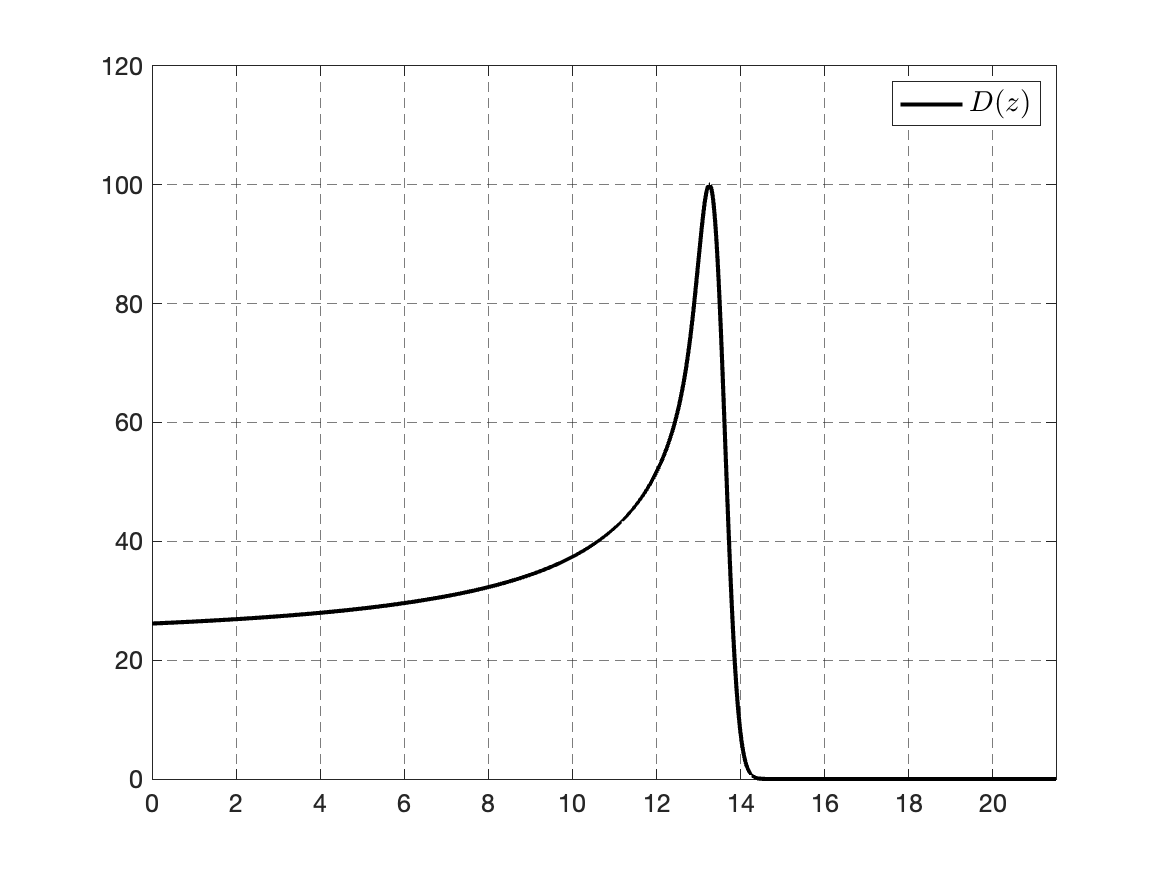
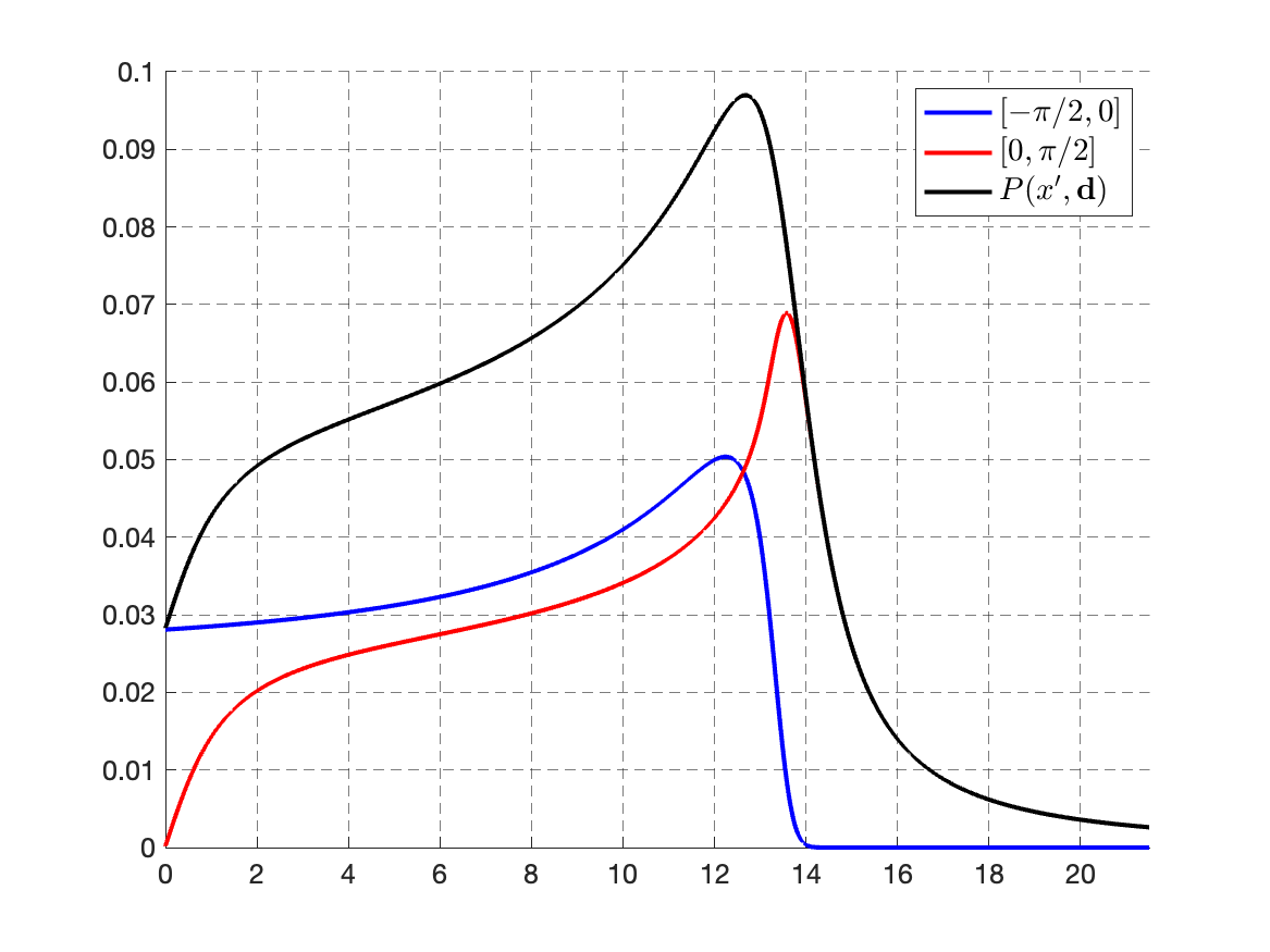
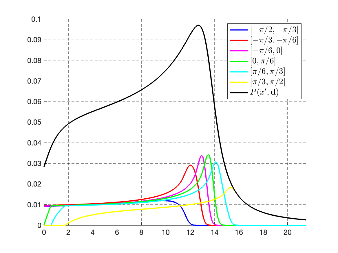
Figure 4. A Bragg Peak (left) and two examples of how the prompt-$\gamma$ distribution $P(x^{\prime}|\boldsymbol{d})$ can be split into two (middle) and six (right) distributions of $\gamma$-detection distributions from coding different emission ranges. In both cases the detectors are positioned at distance $h=1$.

3. Bayesian Inverse Problem

From an operator’s perspective, determining whether the radiation observed by the detectors aligns with a specific patient configuration is crucial. We advocate for a Bayesian modeling approach. Typically, the operator would suggest a prior model for the actual patient configuration during therapy, potentially based on scans taken during the treatment planning phase. After defining this prior, our aim is to utilize the observed radiation profile to assess the likelihood of a successful treatment. As detailed earlier, given a patient configuration, the data distribution can be derived by solving the forward problem. However, we anticipate that solving this forward model with high precision will be numerically demanding. Consequently, we need efficient numerical methods to update our potentially high-dimensional and intricate posterior distribution based on data observations.

We make an assumption that our observations are independent and identically distributed, and the model remains static over time. This challenge falls within the realm of sequential Bayesian learning problems (e.g., [11, Section 3.2]). Our proposal leans towards a model using Sequential Monte Carlo (SMC) methods. Considering the likelihood of configurations being complex and high-dimensional - capturing potential deformations, uncertainties in patient positioning, physical property variations, and more - we aim to design Bayesian methods that explore the prior space effectively while necessitating minimal solutions of the system for specified configurations. In our SMC approach, the posterior measure is represented by a ’cloud’ of potential points, updated based on incoming data. We label these elements in the ’cloud’ as particles; each particle represents a possible patient geometry configuration, requiring a numerical solution of the forward problem.

Broadly, our algorithm, elaborated on further in Section 5 below, adheres to an importance-selection-mutation pattern. In the importance phase, observed data is harnessed to update the posterior probability linked to each particle: particles predicting the data accurately will see a relative boost in their posterior probability, while the others will see a decrease. The selection phase involves rebalancing the particle population-eliminating unlikely particles and duplicating promising ones. The mutation phase introduces particle modifications based on stochastic dynamics. By comparing new and existing particles, an accept-reject step is executed based on prediction accuracy. Without mutation, particles would quickly converge to a few models, hindering the assimilation of extensive data for model refinement. Given the crucial role of mutation, it might be practical to process data in smaller ’chunks’, despite data collection potentially occurring within a brief timeframe. Thus, we suggest a block-sequential data analysis approach, facilitating efficient interplay between selection and mutation.

This method yields a Bayesian posterior probability measure describing the distribution of $\boldsymbol{d}$ given the observed data. Ideally, this could offer insights on treatment outcomes-like posterior estimates of treatment success, potential damage to high-risk zones, or total energy deposition.

For the scope of this paper, we confine ourselves to simpler models with a few input parameters delineated in the preceding section. Our goal is to harness data from the $\gamma$-detectors to estimate values of $\boldsymbol{d}$, subsequently predicting the medium’s properties — possibly tumor position — and dose distribution in the vicinity. By framing this as a sequential Bayesian learning challenge, the posterior probability of a particular configuration $\boldsymbol{d}$ can be articulated when new data points are encountered. Suppose that we observe $k$ $\gamma$-particles at locations $\boldsymbol{x}^{\prime}=(x_{1}^{\prime},\dots,x_{k}^{\prime})$, and want to use this data to infer the likely values of $\boldsymbol{d}$. We can proceed as follows. Using Bayes’ Theorem, the posterior distribution is given as:

(12) $$p(\boldsymbol{d}|\boldsymbol{x}^{\prime})=\frac{p(\boldsymbol{x}^{\prime}|\boldsymbol{d})p(\boldsymbol{d})}{p(\boldsymbol{x}^{\prime})},$$

where $p(\boldsymbol{x}^{\prime}|\boldsymbol{d})$ is the likelihood function, $p(\boldsymbol{d})$ is the prior distribution and $p(\boldsymbol{x^{\prime}})=\int_{\boldsymbol{d}}p(\boldsymbol{d}|\boldsymbol{x^{\prime}})p(\boldsymbol{d})d\boldsymbol{d}$ is the marginal likelihood. In general, $p(\boldsymbol{x^{\prime}})$ is not easily computed, and SMC methods, as described in Section 5 are in large part motivated by the need to avoid the challenge of computing this quantity.

For the prior distribution, we can apply a Gaussian white noise prior on the parameters of $\boldsymbol{d}=\{R_{i},\sigma_{i},\epsilon_{i}\}_{i=1}^{n}$ where the mean and covariances could be chosen to reflect some prior knowledge about $\boldsymbol{d}$ before any observations are made.

The likelihood function is defined using (10) since this equation gives the probability of observing the location $x_{i}^{\prime}$, given a particular choice of the model parameters $\boldsymbol{d}$. Moreover, for $k$ new independent observations, the likelihood is given by

$$p(\boldsymbol{x}^{\prime}=(x_{1}^{\prime},x_{2}^{\prime},\ldots,x_{k}^{\prime})|\boldsymbol{d})=\prod_{j=1}^{k}P(x_{j}^{\prime}|\boldsymbol{d}).$$

Thus, we begin with limited information about the model parameters $\boldsymbol{d}$, represented by the prior. Next, using (12), the posterior is updated by adding $\gamma$-particle readings $\boldsymbol{x}^{\prime}$. This distribution reveals the most likely state of $\boldsymbol{d}$ given $\boldsymbol{x}^{\prime}$ which, at least usually, will become more refined as the number of observations increases, and therefore, giving us a well-informed estimate for $\boldsymbol{d}$. Once these model parameters are established within a certain level of confidence, the physical parameters and the corresponding dose profile can be approximated.

4. KL-based approach to model discrimination

A question of paramount importance to address before practically implementing our methods is the feasibility of distinguishing between two possible patient configurations, especially considering that the data collection will be restricted by the duration of the proton treatment. Further, it’s worth questioning whether enhancing the measurements–by, for instance, increasing the number or sensitivity of gamma detectors or integrating angular sensitivity-would augment our capability to differentiate between successful and unsuccessful treatments. To address this, we employ the Kullback-Leibler (KL) divergence, an information-theoretic perspective on relative entropy, with a focus on its interpretation as discrimination information ([12]).

To simplify our understanding, let us consider wanting to discriminate between just two potential physical configurations. The fundamental query here is: how much data is required to accomplish this? By contemplating two distinct geometries that we might wish to differentiate, we can, in fact, provide estimates on the necessary caliber of the detector setup.

Let us assume we have two closely related probability distributions, $P(x^{\prime}|\boldsymbol{d}_{t})$ and $P(x^{\prime}|\boldsymbol{d}^{*})$, which are the likelihood functions for the true solution and a neighbouring solution respectively. In order to distinguish between the two distributions, the number of observations, $k$, sampled from $P(x^{\prime}|\boldsymbol{d}_{t})$ must satisfy

$$k \geq\left(\log\left(\frac{1-p_{0}}{p_{0}}\right)-\log\left((1-\delta)^{-1}-1\right)\right)$$

(13) $$\quad\quad\quad\quad\quad\quad\times D_{KL}(P(x^{\prime}|\boldsymbol{d}_{t})|P(x^{\prime}|\boldsymbol{d}^{*}))^{-1},$$

where

$$D_{KL}(P(x^{\prime}|\boldsymbol{d}_{t})|P(x^{\prime}|\boldsymbol{d}^{*})) =\int\log\left(\frac{P(x^{\prime}|\boldsymbol{d}_{t})}{P(x^{\prime}|\boldsymbol{d}^{*})}\right)\times P(x^{\prime}|\boldsymbol{d}_{t})dx^{\prime}$$

is the Kullback-Leibler (KL) divergence, $p_{0}$ is the prior probability that $\boldsymbol{d}_{t}$ is true, and $0<\delta\ll 1$ is an acceptable error rate. If the likelihood functions have been split into $b$ bins such that $P(x_{j}^{\prime}|\boldsymbol{d})=\sum_{i=1}^{b}P_{i}(x_{j}^{\prime}|\boldsymbol{d})$, the KL divergence is instead written as

$$D_{KL}(P(x^{\prime}|\boldsymbol{d}_{t})|P(x^{\prime}|\boldsymbol{d}^{*}))=\sum_{j=1}^{b}\int\log\left(\frac{P_{j}(x^{\prime}|\boldsymbol{d}_{t})}{P_{j}(x^{\prime}|\boldsymbol{d}^{*})}\right)\times P_{j}(x^{\prime}|\boldsymbol{d}_{t})dx^{\prime}.$$

If (13) is met, then the posterior probability of the true solution will satisfy

$$p(\boldsymbol{d}=\boldsymbol{d}_{t}|x_{1}^{\prime},x_{2}^{\prime},\ldots,x_{k}^{\prime})\geq 1-\delta,$$

with probability of order 1, which means the truth can be estimated with a high level of confidence.

Suppose we are considering two closely related patient geometries: $\boldsymbol{d}_{t}$ and $\boldsymbol{d}^{*}$. If $\boldsymbol{d}_{t}$ represents the true solution, then to distinguish between these two configurations, the number of observations, $k$, must satisfy the condition given by equation (13). This criterion is influenced by the number of bins, $b$, that the $\gamma$-detectors can discern. Additionally, the sensitivity of the forward model to variations in each of the parameter values plays a crucial role.

Figure 5, with $h=0.2$, illustrates the required number of observations as a function of $b$. From this plot, it’s clear that as $b$ increases, the value of $k$ tends to decrease.

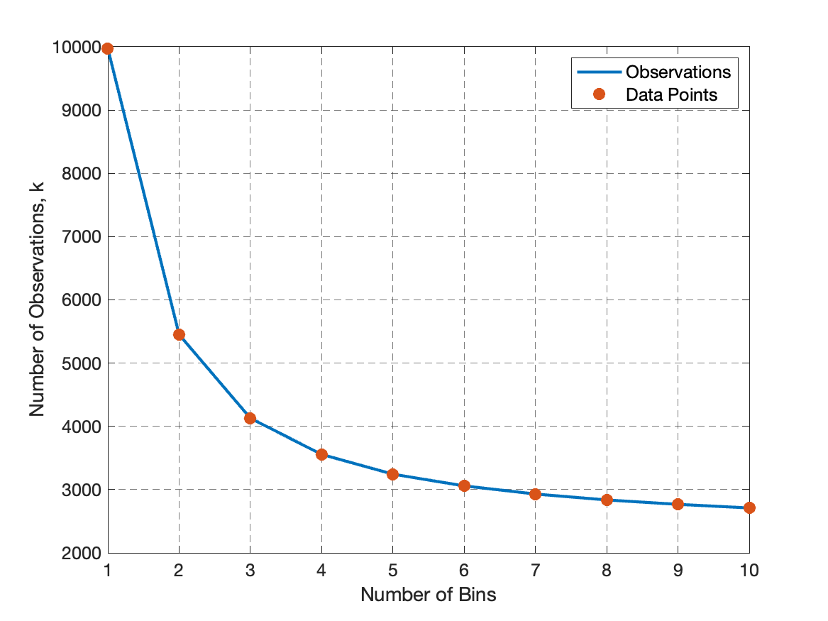
(a) $h=0.5$.

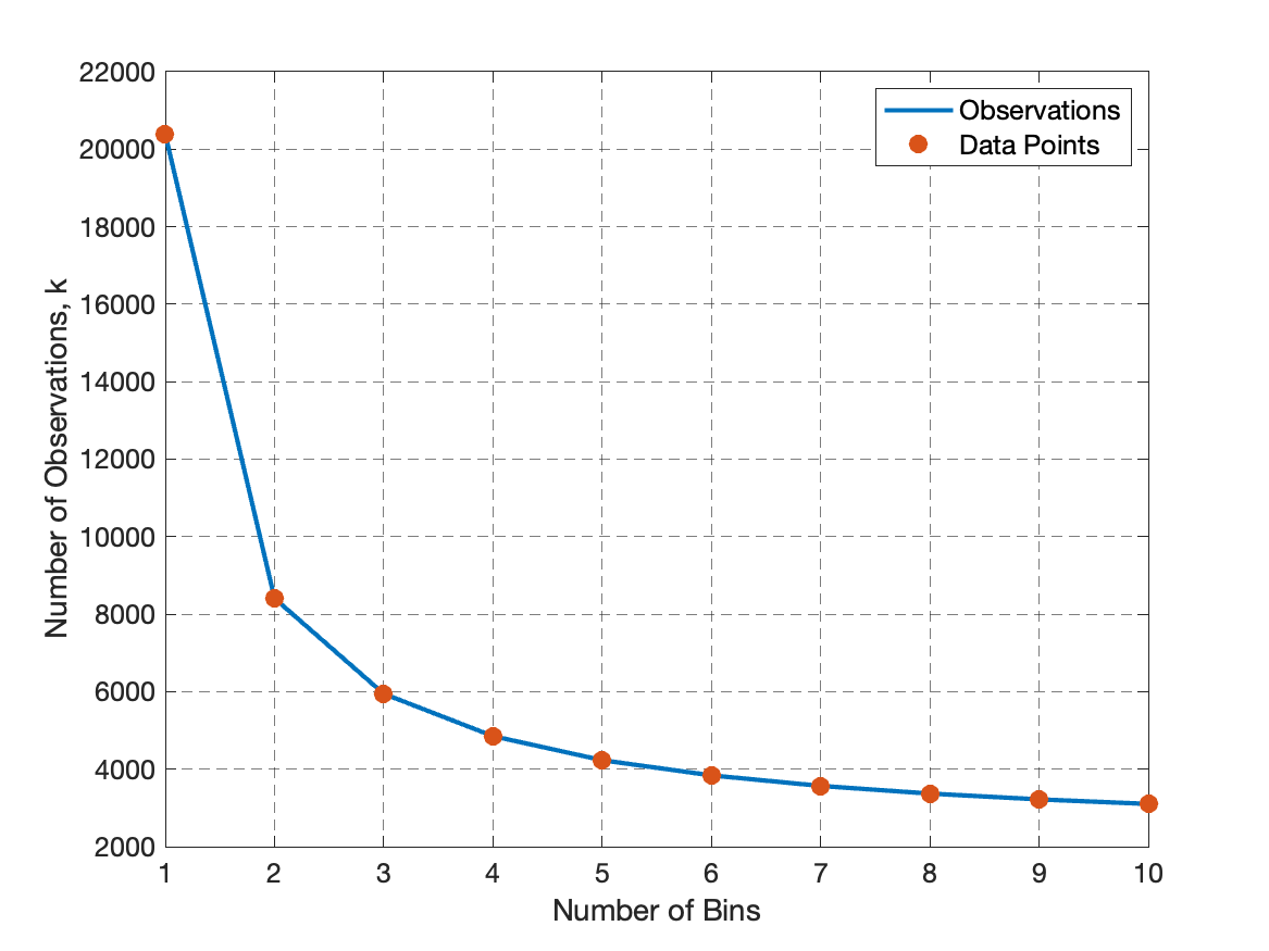
(b) $h=1$.

Figure 5. The number of observations, $k$, needed to discriminate between $\boldsymbol{d}_{t}=(16.2,0.25,0.2)$ and $\boldsymbol{d}^{*}=(16.9,0.3,0.25)$ as a function of the number of bins recognised by the $\gamma$-detectors, for $h=0.5,1$. Here we use the error rate $\delta=0.05$ and prior probability $p_{0}=0.5$.

One can also examine the Kullback-Leibler divergence, $D_{KL}$, for fixed $b$ and as a function of the parameter values, $\boldsymbol{d}$. This enables examination of the sensitivity of the measure to the different parametric values shown in Figure 6.

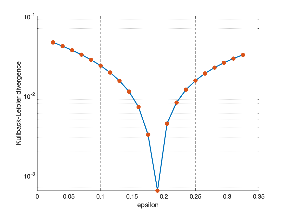
(a) Varying $\epsilon$.

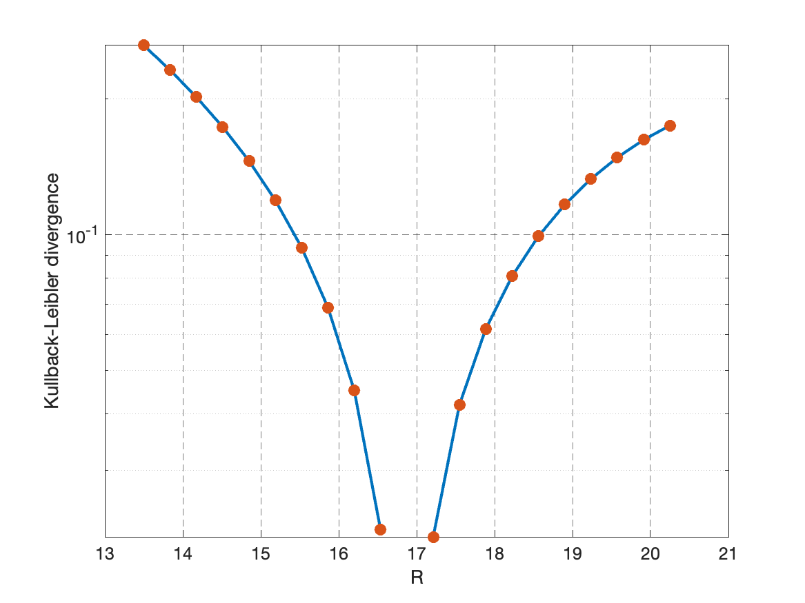
(b) Varying $R$.

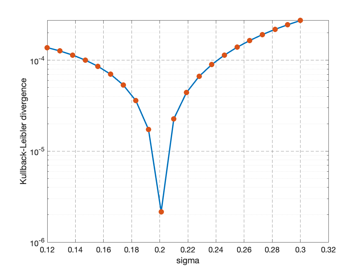
(c) Varying $\sigma$.

Figure 6. Examination of the Kullback-Leibler divergence as a function of individual parameters for a true parameter range $\boldsymbol{d}=(16.9,0.3,0.25)$, a single detector and $h=1$. Notice that the dominant parameter is $R$.

5. Sequential Monte Carlo Approach

Sequential Monte Carlo (SMC) methods have been applied to a wide range of Bayesian problems, and fundamentally rely on simulating a collection of particles whose empirical measure is expected to follow the posterior measure associated with a given data source. Their use was popularised in e.g. [13, 14, 15]. The problem we face can be described as an IBIS (Iterated Batch Importance Sampling) problem ([16], [17, Section 17.2.2]). Our numerical method will be based on using a MCMC (Markov Chain Monte Carlo) step within an SMC algorithm, e.g. [18, Section 3.3.2.3]. To ensure that the proposal distributions from the MCMC step remain viable, we introduce an adaptive MCMC methodology, similar to that proposed in [19].

Since it is difficult to explicitly calculate (12) due to the term $p(\boldsymbol{x}^{\prime})$, which would require integrating over space of possible models, we can instead sample from the posterior distribution using SMC. This involves having $N$ particles that each correspond to some choice of $\boldsymbol{d}=\{R_{i},\sigma_{i},\epsilon_{i}\}_{i=1}^{n}$, sampled from the prior, which are then filtered using importance weights defined by the likelihood function. With additional observations, the particles begin to cluster around the ‘true’ solution, representing a good approximation for $\boldsymbol{d}$. Below we describe the algorithm as we have implemented it, including generating data using a known model (‘truth’). In a genuine implementation, this would be replaced by the actual data observed by the monitoring equipment.

Our SMC approach is detailed below:

1. Truth: Select the ‘true’ values for the model parameters $\boldsymbol{d}^{*}$, and then compute the corresponding ‘true’ probability distribution of (10).

2. Initialisation: For $i=1,2,\ldots,N$, sample $\boldsymbol{d}^{i}\sim p(\boldsymbol{d})$, where $p(\boldsymbol{d})$ is the Gaussian white noise prior.

3. Sample Data: Generate $k$ new observations by randomly sampling from the ‘true’ probability distribution $p(\boldsymbol{x}|\boldsymbol{d}^{*})$.

4. Importance: Given the new observations $x^{\prime}_{j},\;j=1,2,\ldots,k$, for $i=1,2,\ldots,N$, calculate the importance weights

   $$w_{i}=\prod_{j=1}^{k}P(x_{j}^{\prime}|\boldsymbol{d}),$$

   where $P(x_{j}^{\prime}|\boldsymbol{d})$ is given by (10). Then normalise the weights to sum to one by dividing each weight by $\sum_{i=1}^{n}w_{i}$ to obtain $\widehat{w}_{i}=w_{i}/\sum_{i=1}^{n}w_{i}$.

5. Selection: From the set $\{\boldsymbol{d}^{1},\dots,\boldsymbol{d}^{N}\}$, resample with replacement $N$ particles $\{\widehat{\boldsymbol{d}}^{1},\dots,\widehat{\boldsymbol{d}}^{N}\}$ with probabilities $\widehat{w}_{1},\dots,\widehat{w}_{N}$.

6. Mutation: For $i=1,\dots,N$, slightly shift $\widehat{\boldsymbol{d}}^{i}$ in state space. See below for further detail about this step. These perturbed particles are set to $\boldsymbol{d}^{i}$.

7. Repeat: While there is more data, go to step $(iii)$.

To correctly perturb the models in the mutation step, we use a version of a Metropolis-Hastings algorithm, see e.g. [19], detailed below:

1. For $i=1,2,\ldots,N$, sample $\boldsymbol{y}^{i}\sim N(\widehat{\boldsymbol{d}}^{i},C_{i})$, where $C_{i}$ is the covariance matrix for the proposal distribution (a Gaussian distribution has been chosen here).

2. For $i=1,2,\ldots,N$, calculate the acceptance probability

   $$\alpha(\boldsymbol{y}^{i}|\widehat{\boldsymbol{d}}^{i})=\min\left\{1,\frac{p(\boldsymbol{y}^{i})\prod_{j=1}^{k}P(x_{j}^{\prime}|\boldsymbol{y}^{i})}{p(\widehat{\boldsymbol{d}}^{i})\prod_{j=1}^{k}P(x_{j}^{\prime}|\widehat{\boldsymbol{d}}^{i})}\right\}.$$

   This choice of $\alpha$ ensures that the more likely state according to the posterior is selected.

3. For $i=1,2,\ldots,N$, sample $\boldsymbol{d}^{i}$ from $\{\widehat{\boldsymbol{d}}^{i},\boldsymbol{y}^{i}\}$ with probability $\alpha$.

Haario et al. ([20]) proposed a method for computing the covariance matrix such that it varies according to the particle’s path, which they labelled Adaptive Metropolis. Here, to represent the history of the particle, we use the subscript $t$ to correspond to the number of iterations performed. The covariance matrix at iteration $t$ for particle $i$ is defined as

(14) $$C_{i,t}=s_{d}\text{cov}(\widehat{\boldsymbol{d}}_{i,0},\ldots,\widehat{\boldsymbol{d}}_{i,t-1})+s_{d}\delta I_{d},$$

where $s_{d}=(2.38^{2})/m$, $m$ is the dimension of the vector $\widehat{\boldsymbol{d}}_{i}$, $I_{d}$ is the identity matrix and $\delta=0.1$ ensures that $C_{i,t}$ remains positive semi-definite. Note that we only consider the location of the particle after the importance sampling at each iteration. The definition of the covariance matrix for the points $\boldsymbol{X}_{0},\ldots,\boldsymbol{X}_{k}\in\boldsymbol{R}^{d}$ in state space is

$$\text{cov}(\boldsymbol{X}_{0},\ldots,\boldsymbol{X}_{k})=\frac{1}{k}\left(\sum_{j=0}^{k}\boldsymbol{X}_{j}\boldsymbol{X}_{j}^{T}-(k+1)\bar{\boldsymbol{X}}\bar{\boldsymbol{X}}^{T}\right),$$

where $\bar{\boldsymbol{X}}=(1/(k+1))\sum_{j=0}^{k}\boldsymbol{X}_{j}$.

Roberts & Rosenthal ([21]) built upon this work by outlining different extensions to the Adaptive Metropolis technique. One approach involved having two phases for resampling such that

$$\boldsymbol{y}^{i}\sim N\left(\widehat{\boldsymbol{d}}^{i},\frac{0.01I_{d}}{d}\right),\quad\text{for }i\leq 2d,$$

$$\boldsymbol{y}^{i}\sim(1-\beta)N\left(\widehat{\boldsymbol{d}}^{i},C_{i,t}\right)+\beta N\left(\widehat{\boldsymbol{m}}^{i},\frac{0.01I_{d}}{d}\right),\quad\text{for }i>2d,$$

where $\beta=0.05$. The initial phase ensures that mutations do occur during ‘burn-in’. Alternative methods are described in [19], in particular including only implementing the mutation step in an adaptive manner, and may be necessary to reduce computational complexity. Note that we would anticipate that increased dimensionality may also prove challenging (see the discussion in [17, Section 17.2.2]), but could be addressed through the addition of tempering in the algorithm.

6. Numerical results

To highlight the performance and showcase the main ideas behind our methodology, we give a series of numerical examples to test our algorithm. These are designed to investigate the effect of increasing the number of bins, $b$, and the ability to infer tissue density and range verification based on the prompt-$\gamma$ observations.

The accuracy is measured using the mean KL-divergence of the particles,

$$\widehat{KL}=\frac{1}{N}\sum_{j=1}^{N}D_{KL}(P(x^{\prime}|\boldsymbol{d}^{j})|P(x^{\prime}|\boldsymbol{d}^{*}).$$

Here, we always perform twenty iterations of the SMC algorithm, each incorporating additional data, and then assess the prediction accuracy at this point. As a result, all the simulations presented will have roughly consistent computation times.

6.1. Range uncertanties of a pristine Bragg Peak

To begin we consider the case of a pristine Bragg Peak at an energy level of 100MeV through a water phantom. In this case the Bortfeld dose function can be written explicitly with three unknown parametric values, $R,\sigma$ and $\epsilon$. The range of the beam, $R$, is particularly pertinent as it is one of the key uncertainties in proton therapy. We showcase the results of the algorithm presented in Figures 8–9 where the problem is examined with a single detector and six separate detectors respectively. It is worth noting that the algorithm converges significantly quicker when using multiple detectors, although even with a single one the dose is reproduced accurately after twenty SMC iterations.

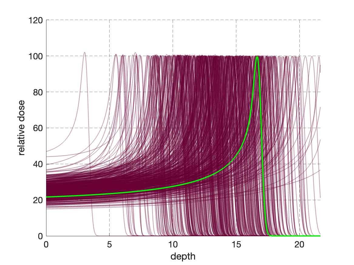
(a) Posterior dose profiles ($Q$) after one SMC iteration.

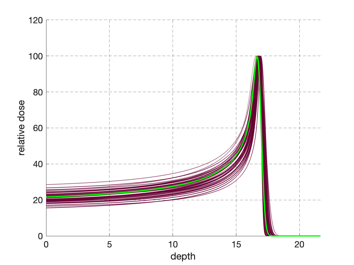
(b) Posterior dose profiles ($Q$) after twenty SMC iterations.

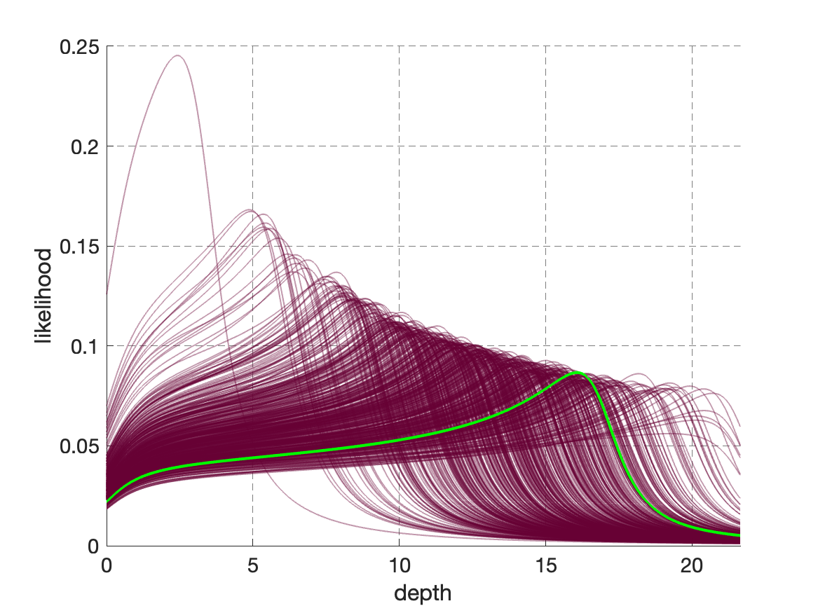
(c) Posterior likelihood functions ($P$) after one SMC iteration.

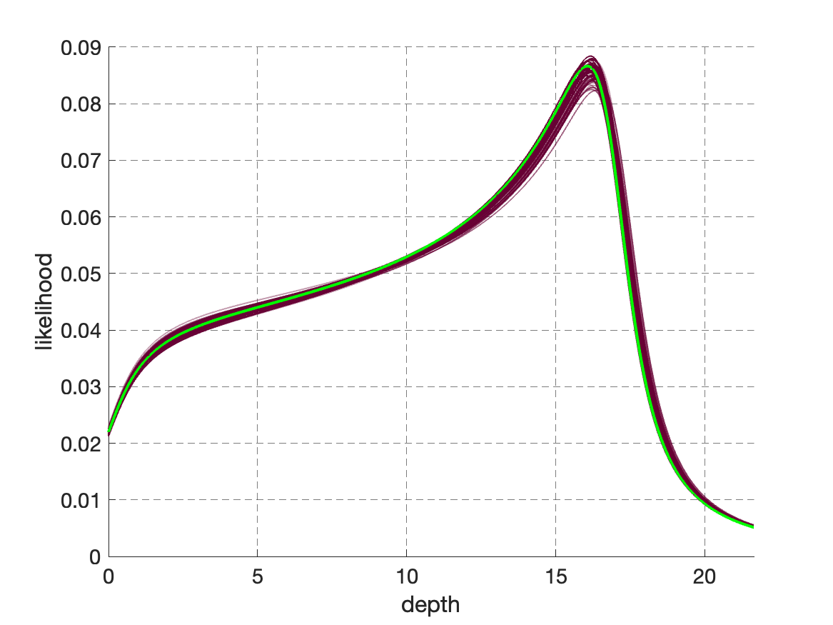
(d) Posterior likelihood functions ($P$) after twenty SMC iterations.

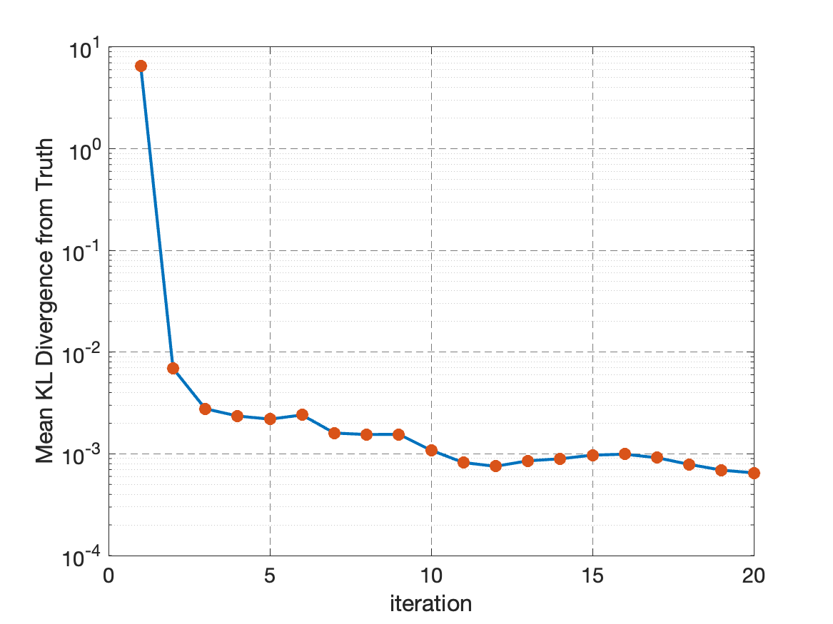
(e) Kullback-Leibler divergence error as a function of SMC iterations.

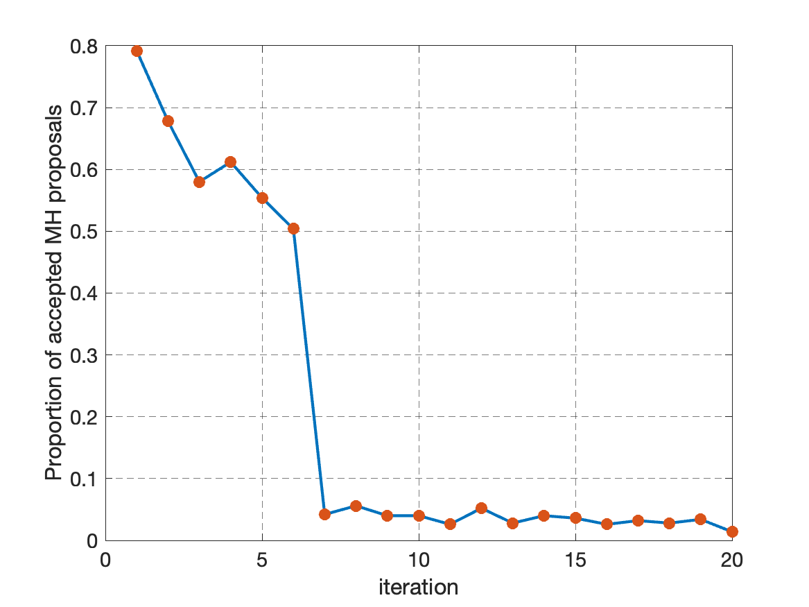
(f) Proportion of accepted Metropolis Hastings proposals as a function of SMC iterations.

Figure 7. The figures above show true and posterior samples of dose profiles (a,b) and observation (c,d) distributions. In (a,b), the green curve denotes the true dose profile, $Q(\cdot|\boldsymbol{d}^{*})$, while the purple curves correspond to $Q(\cdot|\boldsymbol{d}_{i})$ (c.f. (8)) for samples from the posterior distribution. In (c,d), the curves correspond to the true (green) and posterior (purple) observation profiles, $P(\cdot|\boldsymbol{d}^{*})$ and $P(\cdot|\boldsymbol{d}_{i})$ (c.f. (10)) respectively. Plots (a,c) show the posterior distribution after one step of the SMC algorithm, corresponding to $k=1000$ observed $\gamma$-particles. Plots (b,d) correspond to 20 steps of the SMC algorithm, with $10$ times as many observations. Distribution of the particles in $(R,\sigma,\epsilon)$ space is shown in Figure 8.

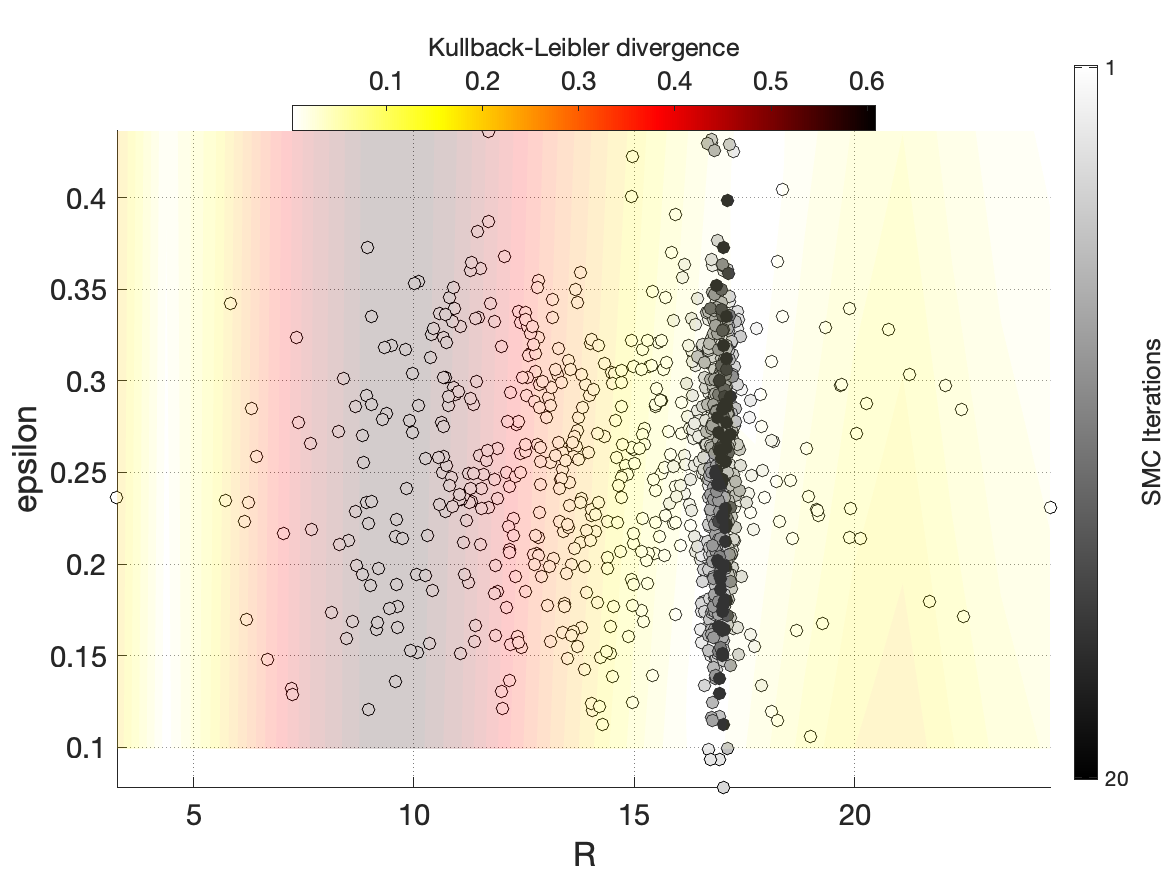
(a) $R$-$\epsilon$ space with a single detector.

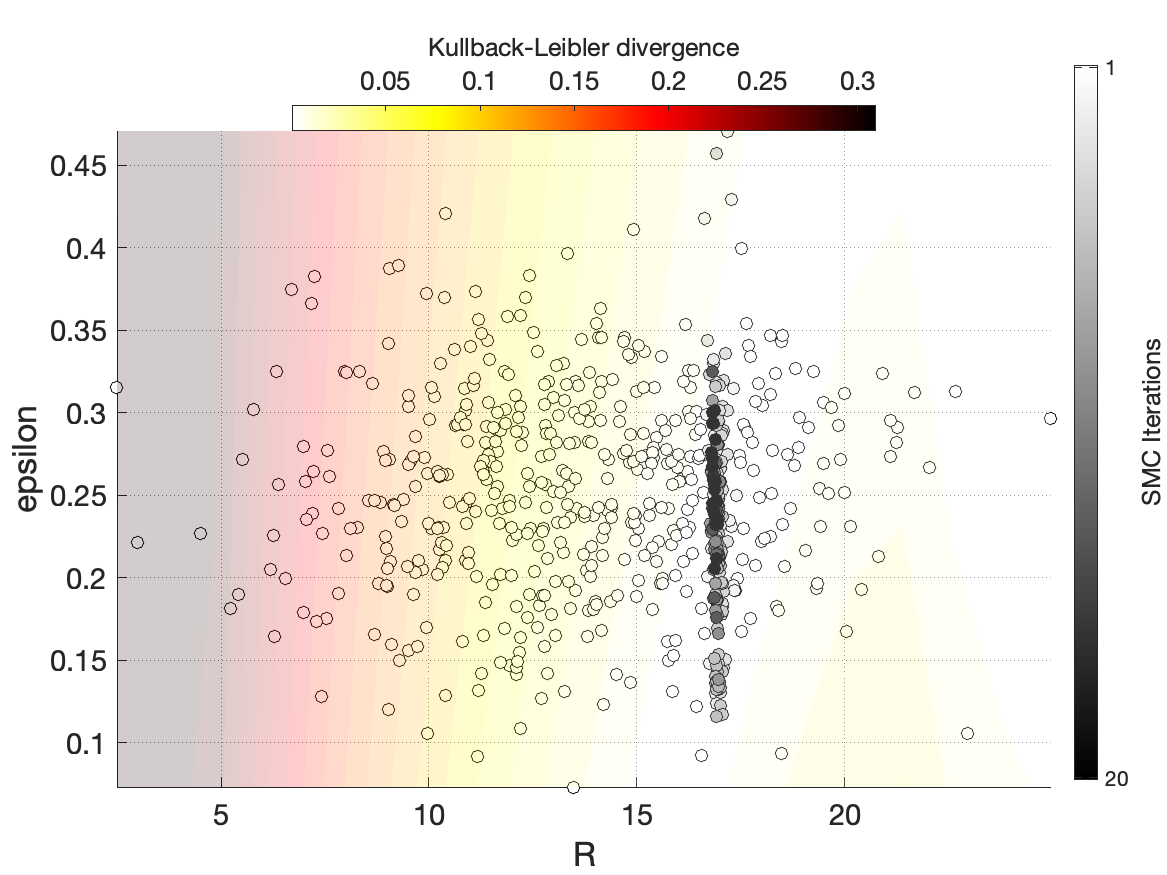
(b) $R$-$\epsilon$ space with six detectors.

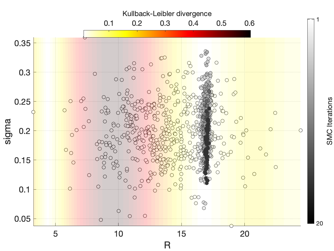
(c) $R$-$\sigma$ space with a single detector.

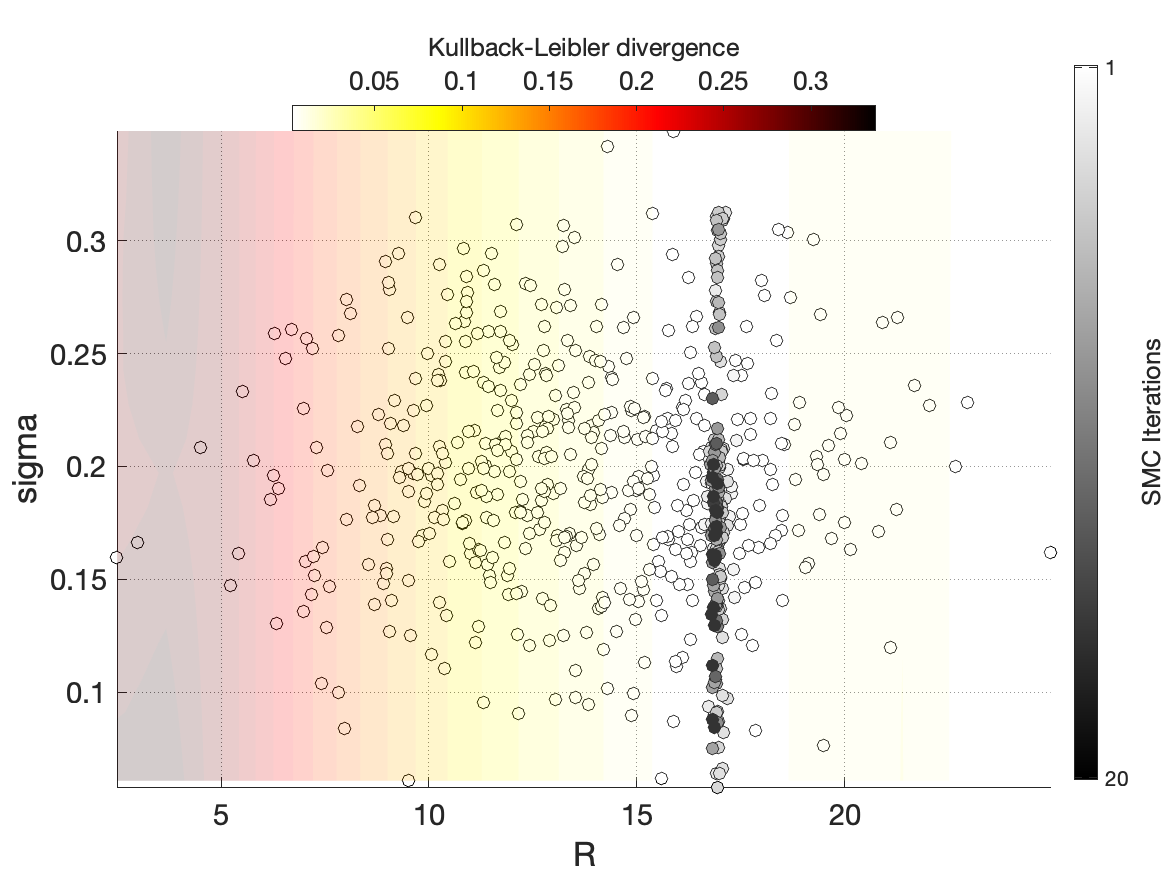
(d) $R$-$\sigma$ space with six detectors.

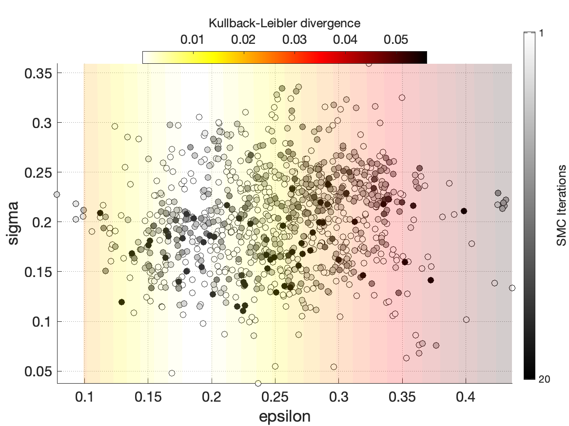
(e) $\epsilon$-$\sigma$ space with a single detector.

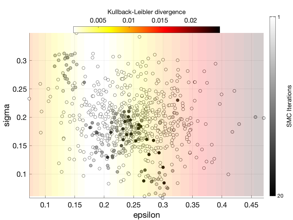
(f) $\epsilon$-$\sigma$ space with six detectors.

Figure 8. Numerical simulation of the SMC algorithm. The points correspond to particles representing parameter values, which concentrate as more data accumulates. Note that the particles are able to clearly identify the range accurately, but are not able to fully resolve uncertainty in the $\sigma,\epsilon$ parameters. The background denotes the KL divergence of the given points relative to the truth. Based on the given scales, it is clear that it is harder for the particles to resolve uncertainty in these parameters against the uncertainty in the range parameter.

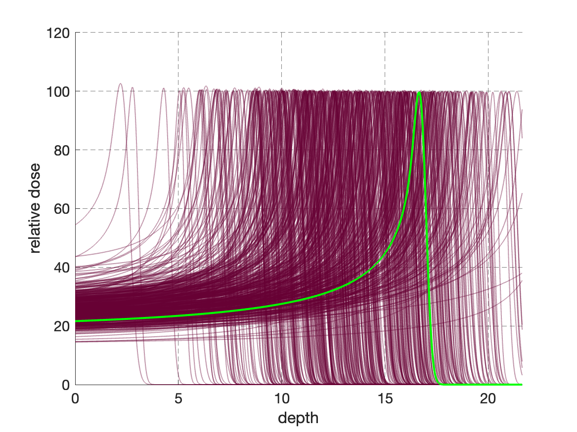
(a) Posterior dose profiles ($Q$) after one SMC iteration.

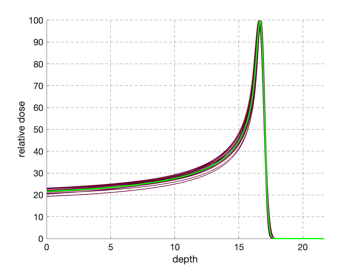
(b) Posterior dose profiles ($Q$) after twenty SMC iterations.

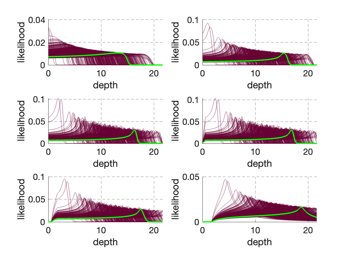
(c) Posterior likelihood functions ($P$) after one SMC iteration.

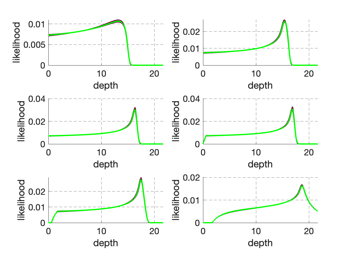
(d) Posterior likelihood functions ($P$) after twenty SMC iterations.

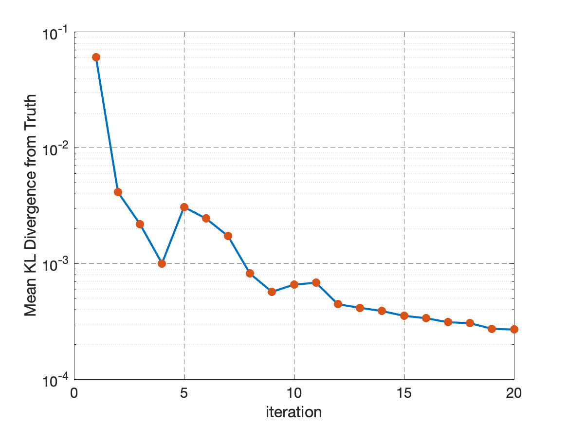
(e) Kullback-Leibler divergence error as a function of SMC iterations.

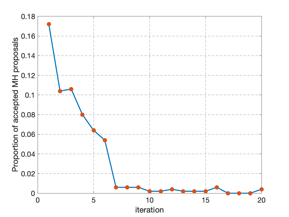
(f) Proportion of accepted Metropolis Hastings proposals as a function of SMC iterations.

Figure 9. This Figure shows the experiment from Figure with the exception that there are six detectors. Notice the algorithm converges significantly quicker and the realisation of dose profile at the twentieth iteration is more accurate than with a single detector.

6.2. Lung tumour

Our second experiment is based on a more challenging setup representing the cross section of a lung tumour. To that end, consider the setup of a one-dimensional cross section given in Figure 10. Notice there are six layers between the proton source, at a $0$cm depth and the tumorous region, between $10-13$cm although there are eleven layers, which is important when considering the impact of range uncertainties. We showcase the results of the algorithm in Figures 11–12 where the problem is examined with a single detector and six separate detectors. Due to the high dimensionality of the parameter space the additional angular resolution with six detectors is important to determine the correct dose deposition.

Figure 10. A one-dimensional lung cross section.

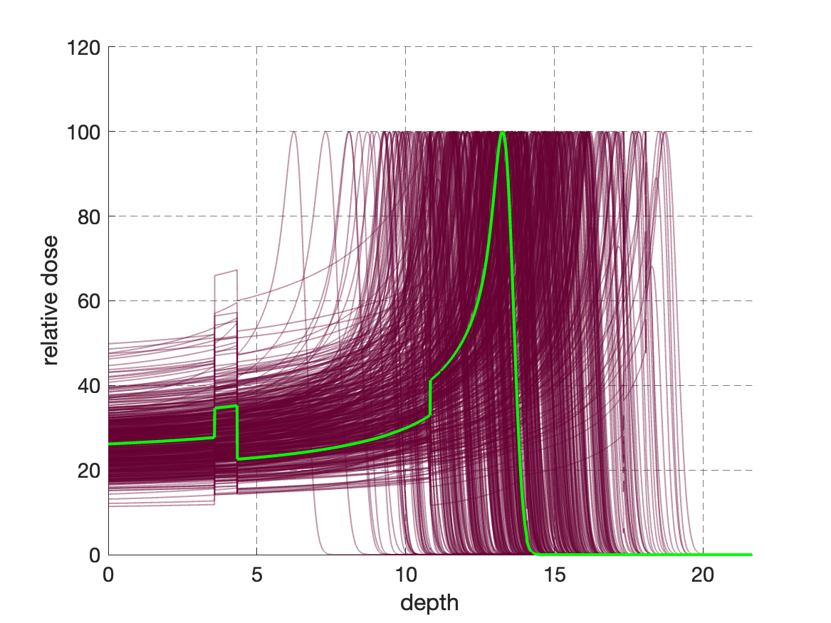
(a) Posterior dose profiles ($Q$) after one SMC iteration.

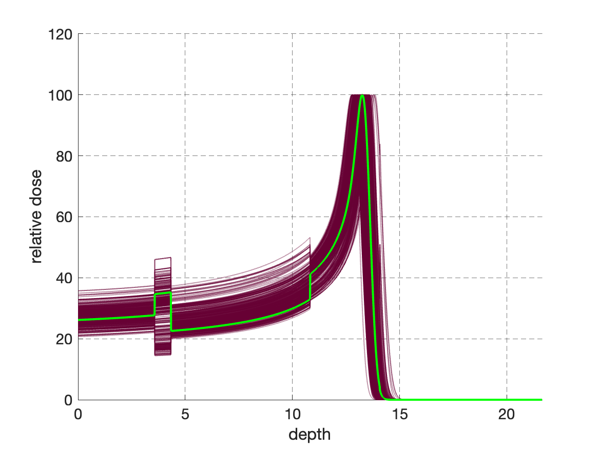
(b) Posterior dose profiles ($Q$) after twenty SMC iterations.

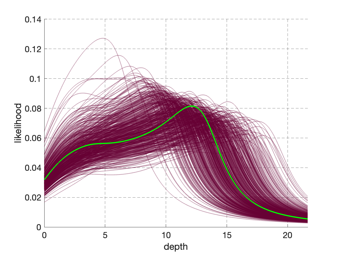
(c) Posterior likelihood functions ($P$) after one SMC iteration.

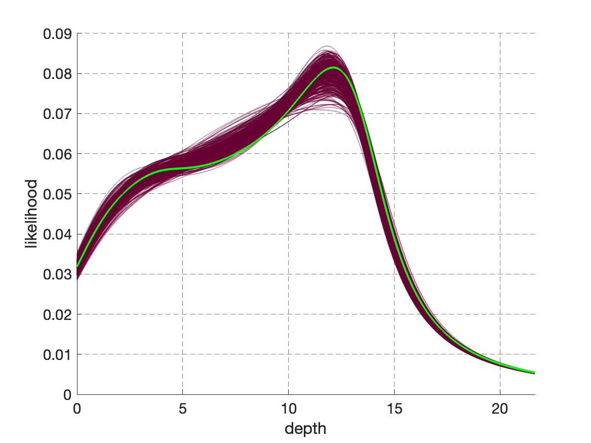
(d) Posterior likelihood functions ($P$) after twenty SMC iterations.

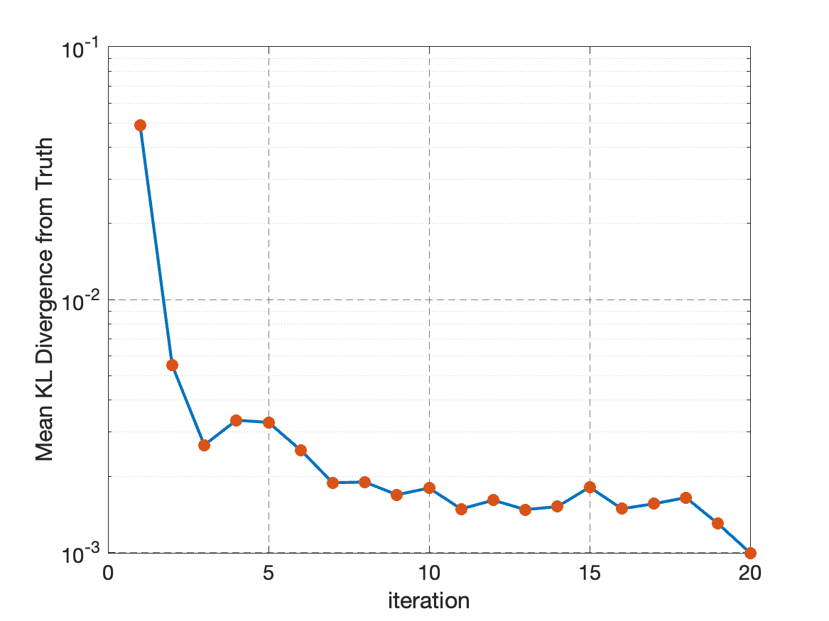
(e) Kullback-Leibler divergence error as a function of SMC iterations.

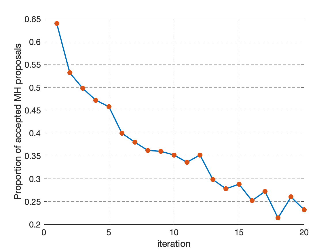
(f) Proportion of accepted Metropolis Hastings proposals as a function of SMC iterations.

Figure 11. The figure shows dose profiles and likelihood functions associated to reconstruction of a Bragg Peak over a lung phantom (§6.2) from observed prompt-$\gamma$ data observed with a single detector. Notice the algorithm does a reasonable job in approximating range however struggles with differentiating between different tissue types.

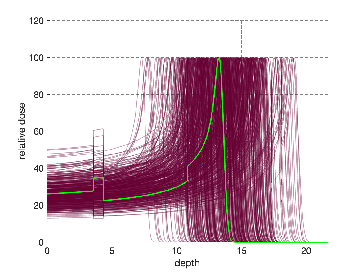
(a) Posterior dose profiles ($Q$) after one SMC iteration.

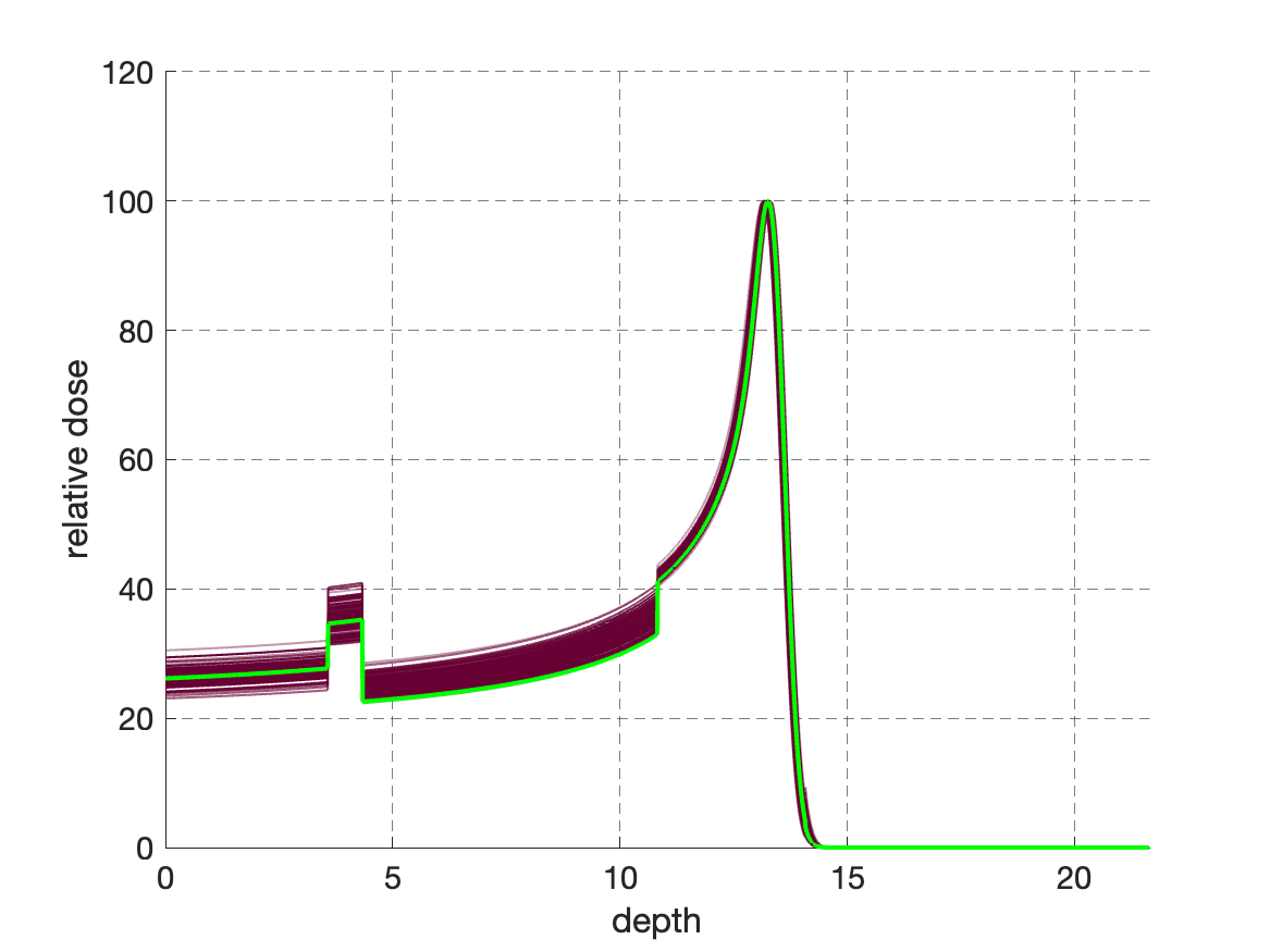
(b) Posterior dose profiles ($Q$) after twenty SMC iterations.

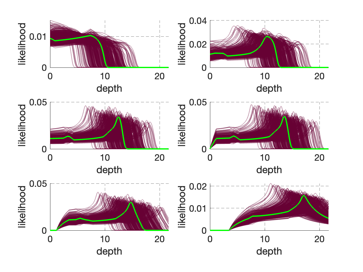
(c) Posterior likelihood functions ($P$) after one SMC iteration.

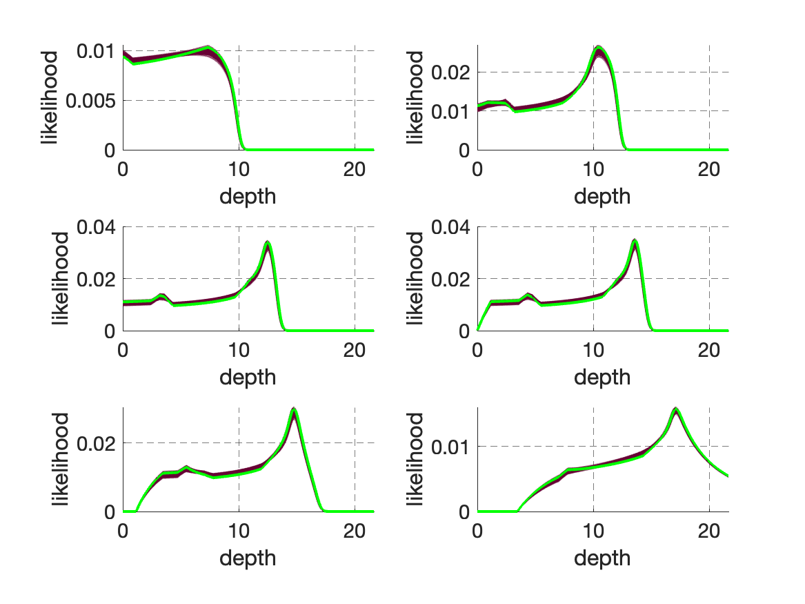
(d) Posterior likelihood functions ($P$) after twenty SMC iterations.

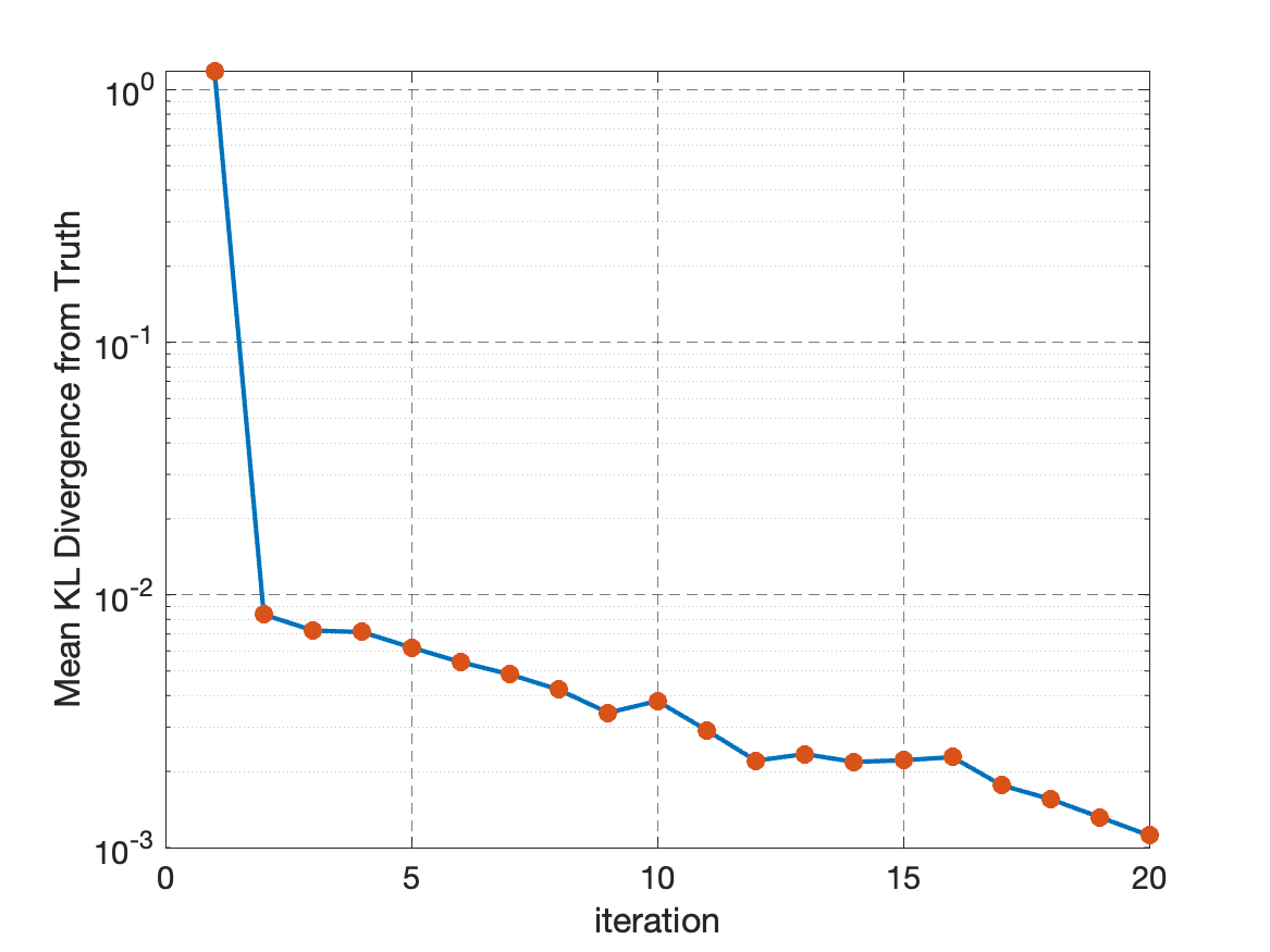
(e) Kullback-Leibler divergence error as a function of SMC iterations.

(f) Proportion of accepted Metropolis Hastings proposals as a function of SMC iterations.

Figure 12. A numerical experiment showing dose profiles and likelihood functions associated to reconstruction of a Bragg Peak over a lung phantom (§6.2) from observed prompt-$\gamma$ data observed with six detectors. Notice the algorithm is well able to approximate the Bragg peak in range and is significantly more accurate in determining tissue profile parameters, however is not able to distinguish sharp transitions between tissue types of high density difference, in this case the transition between bone and lung.

7. Summary and outlook

In this paper we have presented a flexible mathematical framework which could form the basis of future verification methods for PBT. In future work, our framework will enable us to analyse the amount of information required to measure clinically relevant differences, potentially leading to adapted treatment plans, and offers a robust numerical method for providing clinicians with more accurate data on the effectiveness and precision of the delivered treatment.

We anticipate that the methods presented here will play a significant role in the future development of $\gamma$-detectors, and we plan to apply our methods as an integral part of this advancement in future work. Future areas for further work include:

• Recent work ([22]) has developed novel Compton cameras for treatment verification. Compton cameras capture complex information about $\gamma$-radiation, which potentially includes some information about the direction of the observed photon. It should be possible to incorporate this information in a statistically meaningful manner due to the Bayesian elements of our approach. As demonstrated through consideration of different angular decomposition (Figure 5), increased angular resolution should enable more robust discrimination between models. Using the methods presented in this work should make quantifying these benefits straightforward.

• The current approach does not consider noise in the system, due e.g. to background radiation. In practical situations, calibrating these models will be crucial for understanding different noise sources and incorporating them into our updating framework. Similarly, we assume in the setup considered in Figure 10 that the depths of different layers are known. A more realistic scenario might include uncertainty on these depths. The flexible nature of our approach will be important in developing these models.

• An important question for design of future verification systems will be how to optimally place sensors. The work presented in this paper can address this challenge by quantifying various system designs.

• In this paper, we use a relatively simple forward model, which approximates the particle flux using a one-dimensional pencil beam. In practice, more realistic PDE models could be implemented to provide more accurate results. It seems likely that these methods will be significantly more computationally demanding. In the algorithm proposed, each new configuration requires a new numerical solve for the forward model at the given configuration. It seems likely that modified numerical methods, where new particles are introduced at different levels of numerical fidelity, could potentially enhance numerical fidelity in these cases (see, for example, [23]).

Acknowledgements

We would like to thank our friends and colleagues who have generously offered their attention, thoughts and encouragement in the course of this work. We thank Colin Baker and Sarah Osman who kickstarted this work. All authors were supported by the EPSRC programme grant MaThRad EP/W026899/2. Furthermore, AMGC and AEK are grateful for partial support from EP/P009220/1. TP is grateful for partial support from EPSRC (EP/X017206/1, EP/X030067/1) and the Leverhulme Trust (RPG-2021-238).

References

- [1] Lomax AJ, Goitein M, Adams J. 2003 Intensity modulation in radiotherapy: photons versus protons in the paranasal sinus. Radiotherapy and Oncology 66, 11–18. (http://dx.doi.org/10.1016/S0167-8140(02)00308-010.1016/S0167-8140(02)00308-0)
- [2] Particle Therapy Co-Operative Group (PTCOG) Particle Therapy Patient Statistics (per end of 2021). .
- [3] Chen Z, Dominello MM, Joiner MC, Burmeister JW. 2023 Proton versus photon radiation therapy: A clinical review. Frontiers in Oncology 13, 1133909. (http://dx.doi.org/10.3389/fonc.2023.113390910.3389/fonc.2023.1133909)
- [4] Newhauser WD, Zhang R. 2015 The physics of proton therapy. Physics in Medicine & Biology 60, R155.
- [5] Bortfeld T. 1997 An analytical approximation of the Bragg curve for therapeutic proton beams. Medical Physics 24, 2024–2033.
- [6] Stuart AM. 2010 Inverse problems: A Bayesian perspective. Acta Numerica 19, 451–559. Publisher: Cambridge University Press.
- [7] Beskos A, Jasra A, Muzaffer EA, Stuart AM. 2015 Sequential Monte Carlo methods for Bayesian elliptic inverse problems. Statistics and Computing 25, 727–737. (http://dx.doi.org/10.1007/s11222-015-9556-710.1007/s11222-015-9556-7)
- [8] Dunlop MM, Stuart AM. 2016 The Bayesian formulation of EIT: Analysis and algorithms. Inverse Problems and Imaging 10, 1007–1036. (http://dx.doi.org/10.3934/ipi.201603010.3934/ipi.2016030)
- [9] Birmpakos P, Kyprianou A, Pryer T. 2023 A stochastic interpretation of proton bean radiotherapy. Preprint.
- [10] Szymanowski H, Oelfke U. 2003 CT calibration for two-dimensional scaling of proton pencil beams. Physics in Medicine & Biology 48, 861.
- [11] Chopin N, Papaspiliopoulos O. 2020 An Introduction to Sequential Monte Carlo. Springer Series in Statistics. Springer.
- [12] Kullback S, Leibler RA. 1951 On Information and Sufficiency. The Annals of Mathematical Statistics 22, 79–86. Publisher: Institute of Mathematical Statistics (http://dx.doi.org/10.1214/aoms/117772969410.1214/aoms/1177729694)
- [13] Neal RM. 2001 Annealed importance sampling. Statistics and Computing 11, 125–139. (http://dx.doi.org/10.1023/A:100892321502810.1023/A:1008923215028)
- [14] Doucet A, Freitas Nd, Gordon N, editors. 2001 Sequential Monte Carlo Methods in Practice. Information Science and Statistics. New York: Springer-Verlag. (http://dx.doi.org/10.1007/978-1-4757-3437-910.1007/978-1-4757-3437-9)
- [15] Del Moral P. 2004 Feynman-Kac Formulae: Genealogical and Interacting Particle Systems with Applications. Probability and Its Applications. New York: Springer-Verlag.
- [16] Chopin N. 2002 A sequential particle filter method for static models. Biometrika 89, 539–552. (http://dx.doi.org/10.1093/biomet/89.3.53910.1093/biomet/89.3.539)
- [17] Chopin N, Papaspiliopoulos O. 2020 An Introduction to Sequential Monte Carlo. Springer Series in Statistics. Springer.
- [18] Del Moral P, Doucet A, Jasra A. 2006 Sequential Monte Carlo samplers. Journal of the Royal Statistical Society: Series B (Statistical Methodology) 68, 411–436. (http://dx.doi.org/10.1111/j.1467-9868.2006.00553.x10.1111/j.1467-9868.2006.00553.x)
- [19] Fearnhead P, Taylor BM. 2013 An Adaptive Sequential Monte Carlo Sampler. Bayesian Analysis 8, 411–438. Publisher: International Society for Bayesian Analysis (http://dx.doi.org/10.1214/13-BA81410.1214/13-BA814)
- [20] Haario H, Saksman E, Tamminen J. 2001 An Adaptive Metropolis Algorithm. Bernoulli 7, 223–242. (http://dx.doi.org/10.2307/331873710.2307/3318737)
- [21] Roberts GO, Rosenthal JS. 2009 Examples of Adaptive MCMC. Journal of Computational and Graphical Statistics 18, 349–367. (http://dx.doi.org/10.1198/jcgs.2009.0613410.1198/jcgs.2009.06134)
- [22] Perez-Lara ML, Khong JC, Wilson MD, Cline BD, Moss RM. 2023 First Study of a HEXITEC Detector for Secondary Particle Characterisation during Proton Beam Therapy. Applied Sciences 13, 7735. (http://dx.doi.org/10.3390/app1313773510.3390/app13137735)
- [23] Beskos A, Jasra A, Law K, Tempone R, Zhou Y. 2017 Multilevel sequential Monte Carlo samplers. Stochastic Processes and their Applications 127, 1417–1440. (http://dx.doi.org/10.1016/j.spa.2016.08.00410.1016/j.spa.2016.08.004)