Forecast U.S. Covid-19 Numbers by Open SIR Model with Testing

Bo Deng

Abstract: The U.S. Covid-19 data exhibit a high-frequency oscillation along a low-frequency wave for outbreaks. There is no model to account for it. A modified SIR model is proposed to explain this spiking phenomenon. It is also used to best-fit the data and to make forecast. For the simulated duration of 590 days, the model is capable of achieving a 0.5% mean squared relative error (MSRE) fit to the seven-day average of the daily case number. The outright 28-day’s prediction by the model generates a 20% MSRE for the cumulative case total due to a persistent underestimation of the data by the model. With the proposed correction to the abberation, the model is able to keep the 28-day’s cumulative case total forecast within 10% MSRE of the data.

The standard epidemiological model ([3, 20]) for the spread of an infectious disease in a fixed population $N$ is the SIR model:

$$S^{\prime}=-cSI,\ I^{\prime}=cSI-rI,\ R^{\prime}=rI,\ S+I+R=N$$

where $S$ is the number of susceptible at time $t$, $I$ the infected, $R$ the recovered, and $S^{\prime}=S^{\prime}(t)$ is the rate of change (derivative) of variable $S(t)$. Parameter $c$ is the per-infected infection rate and $r$ is the recovery rate. From the onset of Covid-19 pandemic, researchers everywhere shifted into overdrive in search of more realistic models in order to explain the live data and to predict future trend of the pandemic. All models fail by one crucial test. Just a few weeks into the pandemic, it became apparent that the US data exhibit a seven-day oscillation. At first one could dismiss it as an artifact because there are seven days in a week. But after the appearance of the Omicron variant in the summer of 2021, the seven-day oscillation changed to a 3-day oscillation, and the seven-day-a-week explanation dissolved. None of the models I saw in the literature is capable of such oscillations (e.g. [1, 2, 14, 16, 17, 19, 21]). Pandemic forecasting is considered a ‘wicked’ problem by [13] and declared a failure by [10]. The purpose of this article is to present a model and to show how we can fit it to data and then to make reliable forecast on case number and death number.

The SICM Model. There are too many models to list when it comes to Covid-19 modeling. To the SIR model, people can and always do to include many compartments, e.g. exposed, hospitalized, deceased, asymptomatic, young and old, with and without underlying health conditions, etc. Rather than sorting out the pros and cons of such compartments we introduce ours below with minimal comments and leave its justification to how well it can fit and explain the data.

$$\begin{array}[]{l}S^{\prime}=-cSI\\ I^{\prime}=cSI-\frac{pC}{I+aM}I\\ C^{\prime}=\frac{pC}{I+aM}I-mC-dC\\ M^{\prime}=mC-qM\\ R^{\prime}=qM\\ D^{\prime}=dC\\ S+I+C+M+R+D=N_{k}\leq N\end{array}\ \ \begin{array}[]{l}\hbox{ for data fitting:}\\ \quad(k-n_{\rm m})\leq t\leq k\\ \hbox{ for forecasting:}\\ \quad{k}\leq t\leq(k+n_{\rm f})\\ \end{array}$$ (1)

Here, in addition to the susceptible class $S$, the infected class $I$, and the recovered class $R$, we include three more classes: $C$ is for confirmed cases by testing, from which $dC$ many per-day go to the deceased class $D$, and $mC$ many per-day go to the monitored class $M$ for which at least one more test is done in some future days. At a rate of $q$, the monitored comes out from monitoring without further testing and goes into the recovered class $R$. Although we call it the recovered, it is not the conventionally defined recovered class for the basic SIR model. It is rather a subclass but a substantial one. Our $R$ class does not include for example asymptomatic individuals, nor any individual who is tested positive but does not go into monitoring by further testing because of mild symptoms. Notice that a patient who dies from the infection does not receive another test for Covid-19 unlike those in $M$. All assumptions are probabilistic. For example, the last assumption can be stated accurately as that with probability negligible an infected person who died from the infection did not receive another Covid-19 test after their initial diagnosis by testing. Fig.1 gives an illustration of the spiking dynamics of the model (1).

The first date when the Covid-19 case and death numbers was reported for U.S. from CDC’s data is Jan. 22, 2020. The end date for this study is Sept. 1, 2021 ([8]). There is a total of 590 days in between over which our model is fitted to the case and death data. Integer $k$ is between 1 and 590, and is used to denote the $k$th day when forecasting is simulated, also referred to as ‘the forecasting day’, ‘the working day’, the ‘0-day’, or ‘today’ throughout. For the SICM model in the continuous time $t$, we will set the time unit in day so that $t_{k}=k$ automatically.

         

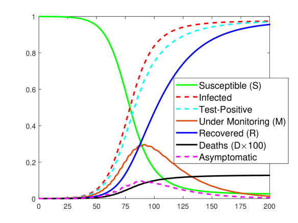
    (a)                                                                        (b)

Figure 1: Model Dynamics: (a) An example of dynamics for the SICM model (1), with parameter values: $c=0.6,\ p=60,\ a=2.2,\ m=7.6,\ d=0.01,\ q=0.05$, and normalized initial values: $S=0.99977,\ I=0.0001,\ C=0.00003,\ M=0.0001$. The ‘infected’ and ‘test-positive’ curves are the cumulative totals for $I$ and $C$ respectively. Their difference is the daily number of asymptomatic. The total deaths is plotted 100 times the actual value $D$ to boost its visibility. (b) Daily numbers ($P$ and $dC$) for the same parameters and initials, with 250 times the daily death number to boost its visibility. Each has its own seven-day average (SDA) curve. All variables are normalized against a total population $S(0)+I(0)+C(0)+M(0)+R(0)+D(0)=N$. The test rate parameter $p=60$ per day per case translates to 24 minutes for test time per case. This sample dynamics is not used to fit any real data.

Our first assumption for the model is that the parameters are not fixed throughout the entire 590-day period because of a variety of reasons: the arises of new variants, behaviour changes as the result of information feedback, changes in mitigation measures, etc. Instead, we assume for each forecasting day, the parameters remain constant only for a duration of $n_{\rm m}$ many days prior to the 0-day. The prior days are referred to as $(-1)$-day for ‘yesterday’, $(-2)$-day for ‘the day before yesterday’, etc. We also assume for each $0$-day, the parameters remain constant for a duration of $n_{\rm f}$ many future days, with $(+1)$-day for ‘tomorrow’ and $(+2)$-day for ‘the day after tomorrow’, etc. We use $n_{\rm m}=21$ days and $n_{\rm f}=28$ days for the study. Thus, for the $k$th-day’s data, there are 22 working days when it is used to fit the model. These are the $(k+0)$th working day for its 0-day’s fit, the $(k+1)$th working day for its $(-1)$-day’s fit, and up to the $(k+n_{\rm m})$th working day for its $(-n_{\rm m})$-day’s fit. In contrast, there are 28 working days when the $k$th-day’s data is a forecasted value. These are the $(k-1)$th working day for its $(+1)$-day’s forecast, the $(k-2)$th working day for its $(+2)$-day’s forecast, and back to the $(k-n_{\rm f})$th working day for its $(+n_{\rm f})$-day’s forecast. Fig.2 gives an illustration on how to organize all data for the study. By definition, a perfect model for a data has the property that for the $k$th-day’s data, all its minus-day’s predicted values and all its plus-day’s fitted values are equal. For every imperfect model, these values are only estimates or approximations of the data. For the illustration of Fig.2 each row of the diary sheet lists things done on a working day, and for the record sheet each row lists things (fitting or forecasting) done to a given day’s data.

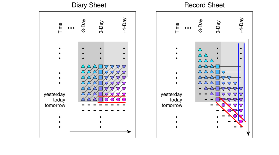
Figure 2: Book Keeping on Forecasting Day: Triangles are for matching, and squares on the 0-Day column are for matching and real data collection on each working day. Upside-down triangles are forecasted numbers, and discs are forecasted numbers done on the working day (‘today’), which then change to upside-down triangles when ‘today’ becomes ‘yesterday’ (or $(-1)$-Day). Entries with a dash are to be filled on future working days. For parameters, each row on the Diary Sheet has one best-fitted value for all ‘$(-)$’ and ‘$(+)$’ days. Each gray line connects all data entries which are either fitted values or forecasted values to a given day’s real data represented by a square on the 0-Day column. For a perfect model, all values connected by a line are identical. The record sheet is a rearrangement of the diary sheet when all values on the slanted lines are rotated clockwise to become horizontal, for which the transformation is referred to as realignment.

The second, and most essential, assumption for our model is that the total population at each given forecasting day is not fixed as the entire U.S. population. This assumption implies that, for example, when the virus first hit New York City, it did not make people from Alaska susceptible instantaneously simply because Alaska is a state of U.S.. In another scenario, if one hunkers down or completely isolates themselves from contacting the virus, then he or she is not part of susceptible, or at best is only a fraction of one susceptible. That is, for each fitting and forecasting period for $(k-n_{\rm m})\leq t\leq(k+n_{\rm f})$, the rolling total population is $N_{k}$, a parameter to be fitted, no greater than the true U.S. population $N$. Because of this assumption, we call our model an open model in contrast to the basic SIR for which $S+I+R=N$, i.e. the sum of $S,I,R$ is closed by the total population. Because the rolling total $N_{k}$ is treated as a parameter for each 0-day, subject to model-to-data fitting like other parameters, the equations for the variables $R$ and $D$ are decoupled from the rest. That is, to fit the model to the data, we only need to compute the first four equations in $S,I,C,M$ in order to find the parameter values and their initial values so that the daily case number and daily death number are best-fitted to the data. For this reason we will refer to our model as the open SICM model or SICM model for short.

The last assumption that is not typically made for extended SIR models is about the daily test-positive rate $P(t)=pCI/(I+aM)$. The justification is based on Holling’s disk function on predation from theoretical ecology ([9, 15, 11, 12]). Holling’s theory, derived for predation, is universal to all processes involving two entities one of which must take time to change the encountering of both into something else. In our setting, Covid-19 testing is an agent or infrastructure which is to find out infected individuals by testing, namely the confirmed class $C$, and to find out if an infected individual under monitoring is free of the virus and thus can be released to the recovered class $R$. For the first class, there is a discovery probability rate $a_{1}$ of the infected class $I$ that will be tested and confirmed. For the second class, there is a repeating test rate $a_{2}$ which is the average number of test an individual will receive over an average period of days under monitoring. For both cases, there is an average time $h$ needed to complete a test. Under these assumptions, the number of daily cases confirmed is the following Holling Type II function

$$\frac{a_{1}I}{1+a_{1}hI+a_{2}hM}C\quad\Rightarrow\quad\frac{(1/h)I}{I+(a_{2}/a_{1})M}C=\frac{pC}{I+aM}I=P$$

where $p=1/h$ is the rate of testing and $h$ is testing time, $a=a_{2}/a_{1}$, the ratio of testing rate for monitored and infected. The number 1 in the denominator is dropped for the reason that the numbers of $I$ and $M$ in the denominator are several orders of magnitude greater. Alternatively, one can start with the assumption that the daily confirmed number is proportional to the product of the infected and the confirmed because one class has a positive feedback on the other class. Because testing takes time, therefore, the daily rate must be constrained by the time allowed and the constraining factor is exactly in the form of the denominator by Holling’s theory. For example, on a day no testing is allocated for the monitored ($a_{2}=0$), and all testing is done for the infected $I$ which is very large. Then as $I\to\infty$, the maximum number of test which the testing infrastructure is capable of completing in a day is $1/h=p$, the daily testing rate unitized by each confirmed case, with the maximal confirmed $pC$ per day. It is the saturation testing rate, implying that when $I$ is large, not every infected can be tested in a fixed time. Letter $p$ for the rate connotes PCR test for the virus.

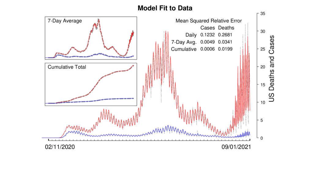
Figure 3: Data-Fitting: The unit for the fitted case number (red) is 1 for $10^{4}$, and the unit for the fitted death number (blue) is 1 for $1.25\times 10^{3}$. For example, the number 4 tick-mark on the scale represents 40,000 for cases and 5,000 for deaths. This false-scale for plot is used to boost the visibility of the death data. All plots use the same case-to-death plot ratio. All dot-dashed curves (gray) are real data.

Data-Fitting. On each working $k$th day, two tasks are performed in sequence. The first task is to solve a nonlinear regression problem to find parameter values and initial conditions so that the model (1) is best-fitted to the data over the past 3 weeks: $(k-n_{\rm m})\leq t\leq k$, with $n_{\rm m}=21$ days. By best-fit it is meant in theory to find the global minimum of an error function. But in practice, there is no practical algorithm to do so. Instead, by best-fit we mean many local minimums with their fitting or regression errors ranked from low to high with the lower the error the better the fit. On each working day, a large number of best-fit searching is carried out and the best 30 results are ranked and archived. All results described below are based on the first 5 best-fits for the 30 saved for each working day, and 541 days in total from Mar. 12, 2020 to Sept. 1, 2021. The reason that the first working day starts on Mar. 12 is because we need to give 21 past days to the first working day to find its best-fits. We could start the first working day earlier but the data from the first couple of weeks were too scattered to be useful.

The searched best-fits are visually represented on the $(-)$-day columns left of the 0-day column on the diary sheet and on the record sheet in Fig.2. Every variable, every parameter, every quantity and number we keep track of such as the daily case number, the daily death number, their seven-day averages (SDAs), cumulative totals, etc., each has one diary sheet as a page to a book. Each book corresponds to one best-fit searching result. Thus, each working day generates a volume of 30 books of diary sheets, and by the same process each working day generates another volume of 30 books of record sheets. All analyses and plots are generated from the record sheet books of the first 5 volumes.

Fig.3 shows the result of how our SICM model is fitted to the U.S. case and death data. Here is how the graph is assembled. All are based on the daily numbers for cases and deaths. Take the main daily-case fitting curve for example. For each point $k$ on the horizontal axis corresponding to the $k$th-day, we first find the average of the entries from the $k$th-day row and left of the 0-day column on the daily-case record sheet for each best-fit volume $1\leq i\leq 5$, and then average the 5 averages to obtain the plot value for the fitted daily-case number. Connect these dots from day 50 to day 590 to obtain the spiking daily-case curve. Once the daily-case sequence is obtained, the SDA is generated by averaging the past 7 days’ daily-case numbers for each $k$th-day. Similarly, the cumulative total is generated by summing all past days’ daily-case numbers to day-$k$ for each $k$th-day. The same operations are applied to obtain these types of curves for deaths. These definitions for daily number time sequences, SDA number time sequences, and cumulative total time sequences will be used throughout for both fit and for forecast analyses and plots.

The definition for the mean squared relative error (MSRE) is defined as follows. Let $\delta=\{\delta_{1},\delta_{2},\dots,\delta_{n}\}$ denote any data sequence, such as the daily-case data, the SDA data, or the cumulative total data, etc. Let $\phi=\{\phi_{1},\phi_{2},\dots,\phi_{n}\}$ denote any fit or forecast sequence of the same type. Then the MSRE between the fit and the data is defined as

$$E(\phi,\delta)={\rm mean}\{|\phi_{i}-\delta_{i}|^{2}/\delta_{i}^{2}:1\leq i\leq n\}=\frac{1}{n}\sum_{i=i}^{n}{|\phi_{i}-\delta_{i}|^{2}}/{\delta_{i}^{2}}$$. (2)

Fig.3 shows, for example, the MSRE for the daily-case is 12.32%, for the SDA is 0.5%, and for the total is 0.06%, over the time period from day 50 to day 590. MSRE measures the squared relative error per datum on average.

The method for best-fit is based on Newton’s gradient search (Methods and [4, 5, 18]). It is to find the parameter and initial values of the SICM model so that the MSRE for the joint daily case and daily death between model’s solution and the data (over the fitting period from $k-n_{\rm m}$ to $k-0$ ) is a minimum. As mentioned before, only 30 best-fits are ranked and archived.

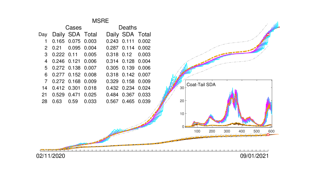
Figure 4: Coat-Tail Plot: Dashed lines are for real data. Thin dash-dot lines outline the $\pm$10% bounds off the real data. The same conventions apply to all plots. All ‘Mean’ errors for the paper are MSRE. The main graph for cumulative totals shows the primary projections four-weeks ahead each working day. But the insert for the SDA coat-tail projection shows only two-weeks ahead each working day. Not all 28 projected curves are plotted for a better visibility. For both total and SDA, the first curve is for the $(+3)$-day projection, and then every 3rd day projection thereafter. For the main plot, the last curve ends wit the $(+27)$th-day’s projection and for the insert it ends with the $(+15)$th-day’s SDA.

Coat-Tail Plot – Forecaster’s Trap. On any given $k$th working day, the second task following best-fitting is to make a forecast on daily case and death numbers $n_{\rm f}=28$ days into the future. By definition, all preparatory analyses are referred to as projections, and only the final projection is called the forecast. All projections are based on the columns right of the 0-column on the record sheets (c.f. Fig.2).

The first type projection is called the primary projection or Type-I projection. It is simply the continuation of solution of the best-fitted SICM model 28 days ahead for each $k$th forecasting day. All types of numbers are functions of of the daily numbers.

Take the daily cases for example. Instead of stopping at the working day $k$, we define

$$\chi_{cs,k,i}(+j)=P_{i}(k+j),\quad 1\leq j\leq n_{\rm f}$$ (3)

to be the Type-I projection, where $P_{i}(t)$ is the model’s daily cases projected into the future on the $k$th forecasting day for the $i$th best-fitted search, and the first subscript $cs$ is for ‘cases’. By extension, we will use $\chi_{ds,k,i}(+j)=d_{i}C_{i}(k+j)$ for the daily deaths with the subscript $ds$ for ‘deaths’, and later $\chi_{x,k,i}(+j)=x_{i}(k+j)$ for any of the variables $x=S,I,C,M$, etc. The plus sign ‘$+$’ is used to emphasize the fact that the quantities are projected future values.

Assume the primary projection is forecasted. The question for everyone, the forecaster and all observers, is how good is the forecast? To this question there lies a forecaster’s trap epitomized by what is referred to as a coat-tail plot as shown in Fig.4. Take the cumulative total plot for cases for example. On a forecasting day $k$, the forecaster uses the known $k$th-day’s data $\delta_{t,cs,k}$, with the first subscript $t$ for ‘cumulative total’, and then add up the projected daily numbers to obtain the total for each best-fit $i$:

$$\psi_{t,cs,k,i}(+z)=\delta_{t,cs,k}+\sum_{j=1}^{z}\chi_{cs,k,i}(j)$$

for $1\leq z\leq n_{\rm f}$ and $1\leq i\leq 30$. Average over $1\leq i\leq 5$ to obtain the forecasted cumulative total

$$\psi_{t,cs,k}(+z)={\rm mean}\{\psi_{t,cs,k,i}(+z):1\leq i\leq 5\}.$$

There are 28 projected curves for the cumulative total. For the $(+1)$-day projection curve, the plotted point for the $k$th-day is $\psi_{t,cs,k-1}(+1)$ because it is projected on the $(k-1)$th working day. In general, For the $(+z)$-day projection curve for $1\leq z\leq 28$, the plotted point for the $k$th-day is $\psi_{t,cs,(k-z)}(+z)$ because it is projected on the $(k-z)$th working day. As for the MSRE, it is calculated as $E(\psi_{t,cs,\cdot-z}(+z),\delta_{t,cs,\cdot})$ where the $\cdot$ denotes the position index for elements of the sequences, $50\leq j\leq 590$. The MSRE does not accumulate because the projected sequence and the data sequence are the same for $j<(k-z)$.

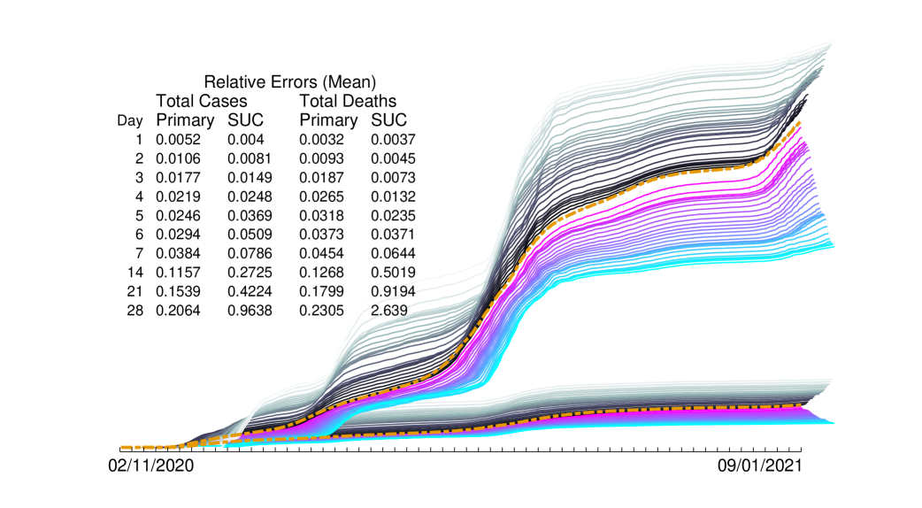
Figure 5: Observer’s Plot and Abberations: Colored curves are from the primary (Type-I) projections, with curves closer to the real data being projections closer to the 0-day. Graded-gray curves (Type-II projection) are generated by the Step-Up Correction to the primary projection, with darker the shade the closer to the 0-day. The primary projection is an underestimate abberation and the SUC is an overestimate abberation.

For the SDA plot in Fig.4, similar coat-tail construction applies. Take the case number for example. We start by considering the solution of the best-fitted model over the time interval spanning both the matching window and the projecting window, followed by computing the SDA

$$\psi_{s,cs,k,i}(+z)={\rm mean}\{P_{i}(k+j):z-6\leq j\leq z\},\ \hbox{ for $1\leq z\leq n_{\rm f}$}$$

where $P_{i}$ is the same daily cases function for the $k$th-day’s best-fit number $i$, $1\leq i\leq 30$. For the plot, the $k$th-day’s SDA point is the averaged value over the first 5 best-fits with projection made on the $(k-z)$th working day:

$$\psi_{s,cs,(k-z)}(+z)={\rm mean}\{\psi_{s,cs,(k-z),i}(+z):1\leq i\leq 5\}.$$

Once the SDA curve is obtained, the mean error can be computed against the SDA real data $\{\delta_{s,cs,j}:50\leq j\leq 590\}$ as we do for the cumulative total.

The coat-tail forecast is a subjective, forecaster-centric way to promote the forecaster’s methodology. It is prevalent in the literature (e.g. [6, 16]). It is easy to see from the illustration Fig.4 that a coat-tail plot can be generated on any day without reaching deep into the past. Its projection is attached to the forecaster’s model-fitting black box – all columns left of the 0-day column, and hence the ‘coat-tail’ moniker. The coat-tail projections on the SDA and cumulative total do not accumulate in errors, which always result in a bias forecasters often fail to recognize.

Observer’s Plot and Abberations. To evaluate the performance of a projection, there is another way other than the coat-tail plot preferred by the forecaster. It is the observer’s plot. To evaluate how good a $(+7)$-day forecast is, for example, an observer only needs to compare all $(+7)$-day forecasts by the forecaster to the actual data. Take the cumulative total for cases as an example again. This is to compare the actual data sequence $\delta_{t,cs,k}$ with the projected data $\phi_{t,cs,(k-z)}(+z)$ with $z=+7$ for all past forecasting days where

$$\phi_{t,cs,(k-z)}(+z)={\rm mean}\{\phi_{t,cs,(k-z),i}(+z):1\leq i\leq 5\}$$

and

$$\phi_{t,cs,(k-z),i}(+z)=\sum_{j=z+1}^{k+z}\chi_{cs,(j-z),i}(+z)$$ (4)

where $\chi_{cs,j,i}(+t)$ is the working $j$th-day’s projected daily cases from definition (3). The curve $\{\phi_{t,cs,(k-z)}(+z):(z+1)\leq k\leq 590\}$ with $z=+7$ by definition is the observer’s plot for forecaster’s $(+7)$-day performance, and the MSRE is computed similarly by

$$E_{t,cs}(+z)={\rm mean}\{(\phi_{t,cs,(j-z)}(+z)-\delta_{t,cs,j})^{2}/\delta_{t,cs,j}^{2}:(z+1)\leq j\leq 590\}$$

for $z=+7$. The observer’s evaluation on any other $(+z)$-day’s forecast for $1\leq z\leq n_{\rm f}$ is done similarly. In particular, the SDA for cases, for example, is given by

$$\phi_{s,cs,k,i}(+z)={\rm mean}\{\chi_{cs,j,i}(+z):k-6\leq j\leq k\},\ k\geq 7$$

for each best-fit $i\leq i\leq 30$. For each $1\leq z\leq n_{\rm f}$ the $\phi$ curves as time series in $k$ are referred to as the observe’s curves for the $(+z)$-day.

Fig.5 contains all 28 primary projections for case total and 28 primary projections for death total, with e.g. $E_{t,cs}(+7)=0.0384$. For the $(+28)$-day projection, the MSRE is $E_{t,cs}(+28)=0.2084$, but from the plot we can see that for many parts of the curve, the error is way greater than 20%, pushing to 40% and 50%. In comparison with its coat-tail counterpart from Fig.4, the $(+28)$-day’s projection error is only 5% on average and rarely exceeds the $\pm 10$% envelope. To summarize, an observer’s curve must be generated deep into the past, without connection to forecaster’s ‘black box’, and without constant resetting by the forecaster to the real data like its coat-tail counterpart does, its error from the real data almost always accumulates.

But the type of error we see from observer’s plots is not random. Instead, it is a rather simple abberation because the $(+)$-day projection for the cumulative totals is a consistent deviation from a norm, namely the data. Specifically, each curve is an under-estimate of the data, apparent from the very beginning, an insight extremely useful for the forecasters, and the further ahead of the projection the greater the deviation for the projection from the data. Like all abberations, it can be corrected to various degrees.

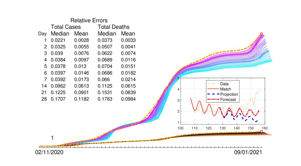
Figure 6: Abberation-Corrected Projection: The AAC projection (Type-III) for most of the working days is an under-abberation. The $b$ value is $b=1$, at the bottom left corner. The median error is defined as the median of the relative errors: ${\rm median}\{|\phi^{1}_{t,y,j-z}(+z)-\delta_{t,y,j}|/\delta_{t,y,j}:50\leq j\leq 590\}$ for $y=cs,\ ds$. Insert is for a sample result for the case numbers from the 128th working day: showing the model-fitted curve to data (solid red), the Type-I projection (dashed blue), and the Type-III forecast (dot-dashed red).

Boosted Abberation Corrections for Forecast. The second type projection (Type-II) is called the step-up-correction (SUC) projection. It is based on the cumulative totals for the data $\delta_{t,y,k}$ and for the primary projection $\phi_{t,y,(k-z)}(+z)$, $y=cs,ds$. We will use the superscript ‘$suc$’ to denote such projections. Take the cumulative total for the cases for example. Because the primary projection for $(+z)$-day, $\phi_{t,cs,(k-z),i}(+z)$ is an underestimate of the real data, $\delta_{t,cs,k}$, c.f. Fig.5, the idea is to correct the abberation by lifting up the projection. As always, we start with the daily case number, $\chi_{cs,k,i}(+z)$, which is scaled up by a compensating factor which is the ratio of data to projection in the case totals:

$$\chi^{suc}_{cs,k,i}(+z)=\frac{\delta_{t,cs,k}}{\phi_{t,cs,(k-z)}(+z)}\chi_{cs,k,i}(+z)$$

on the $k$th forecasting day for all $1\leq z\leq n_{\rm f}$ with $\chi$’s definition from (3). Similarly, we will extend the definition to all variables $x=S,I,C,M$ $\chi^{suc}_{x,k,i}(+z)=[\delta_{t,cs,k}/\phi_{t,cs,(k-z)}(+z)]\chi_{x,k,i}(+z)$, except for the daily death number which is defined as

$$\chi^{suc}_{ds,k,i}(+z)=\frac{\delta_{t,ds,k}}{\phi_{t,ds,(k-z)}(+z)}\chi_{ds,k,i}(+z)$$

We can then define the SUC for $\phi^{suc}_{t,cs,k,i}(+z)$ the same as we do in (4) and

$$\phi^{suc}_{t,cs,(k-z)}(+z)={\rm mean}\{\phi^{suc}_{t,cs,(k-z),i}(+z):1\leq i\leq 5\}$$

and the MSRE $E^{suc}_{t,cs}(+z)$ similarly as for $E_{t,cs}(+z)$ as above. We can also define similarly for SDA related quantities: $\phi^{suc}_{s,cs,(k-z)}(+z)$, $E^{suc}_{s,cs}(+z)$, etc. And similarly for the death numbers and MSREs by substituting the subscript $cs$ by $ds$. Fig.5 also shows the $\phi^{suc}$ curves for the cumulative totals for cases and deaths. It also shows that the MSRE $E^{suc}$ is worse off for $(+)$-days further away from the 0-day. Fortunately, the SUC projection is again an abberation. But this time it is an overestimate abberation, which again is subject to corrective intervention.

Figure 7: Forecasting: Use different boosted AACs to make the daily forecast. From day 50 to day 185, $b=3$ is used, from day 186 to 275, $b=1$ is used, and the subsequent switching takes place on day 325, 550 with the $b$ value equal 2, 3, respectively. The main plot is the cumulative totals for all 28 days. Insert shows the corresponding SDA forecast, plotted every plus-three days for 15 days ahead on each working day. Daily forecast is not shown but their daily variations are comparable with their SDA counterparts as shown in the MSRE table.

The Type-III projection is referred to as averaged-abberation-correction (AAC) or boosted AAC, and we will use a superscript value ‘$b$’ to denote such projections. Again, take the cumulative total for cases as example and start with the daily case number. The AAC projection for the daily number on the $k$th-forecasting day is to apply a weighted-average to the primary under-abberation projection and the SUC over-abberation projection as follows

$$\chi^{1}_{cs,k,i}(+z)=\frac{\tau_{(k-z)}(+z)\chi^{suc}_{cs,k,i}(+z)+\tau^{suc}_{(k-z)}(+z)\chi_{cs,k,i}(+z)}{\tau_{(k-z)}(+z)+\tau^{suc}_{(k-z)}(+z)}$$ where (5)

$$\tau_{(k-z)}(+z)=\phi_{t,cs,(k-z)}(+z) \tau^{suc}_{(k-z)}(+z)=\phi^{suc}_{t,cs,(k-z)}(+z)$$ and . (6)

That is, the daily over-abberation is weighted by the primary under-abberation total and the daily under-abberation is weighted by the SUC over-abberation total. Here $b=1$ for this AAC. We can then use the AAC daily case numbers to define $\phi^{b}_{t,cs,(k-z)}(+z)$ and $E^{b}_{s,cs}(+z)$ for $b=1$, etc. As shown in Fig.6, the AAC is a substantial improvement over the Type-I and the Type-II projections. For example, the (+28)-day projection’s MSRE for the cumulative case total is only 11.8% and that for cumulative death total is below 10.0%.

Because this AAC projection for the case total with $b=1$ is still an under-estimate abberation, the SUC projection for the case total can afford to be an even greater over-abberation. We can do this by scaling up the weight $\tau^{suc}_{(k-z)}(+z)=\phi^{suc}_{t,cs,(k-z)}(+z)$ in (5) by a boosting factor. Specifically, let $b$ be $b\geq 1$ and for any $(+)$-day number $+z$, $1\leq z\leq n_{\rm f}$, define the incremental boosting factor as

$$\beta(+z)=1+\Delta_{b}(z-1),\ \hbox{ where $\Delta_{b}=\frac{b-1}{n_{\rm f}-1}$}$$

so that $\beta(+1)=1$ is for no boost, $\beta(+2)=1+\Delta_{b}$ is for one $\Delta_{b}$ boost, etc, and $\beta(+n_{\rm f})=b$ is for the full $b$ amount boost as $1\leq\beta(+z)\leq b$. The daily case number for the boosted AAC projection with $b\geq 1$ is

$$\chi^{b}_{cs,k,i}(+z)=\frac{\tau_{(k-z)}(+z)\chi^{suc}_{cs,k,i}(+z)+\beta(+z)\tau^{suc}_{(k-z)}(+z)\chi_{cs,k,i}(+z)}{\tau_{(k-z)}(+z)+\beta(+z)\tau^{suc}_{(k-z)}(+z)}$$ (7)

which generalizes the definition (5) to any value $b\geq 1$. From these boosted daily case numbers we can define the corresponding boosted AAC projection for the case total $\phi^{b}_{t,cs,(k-z)}(+z)$ and its MSRE $E^{b}_{s,cs}(+z)$ for $b\geq 1$. The same can be done for the boosted AAC projections on the daily death number

$$\chi^{b}_{ds,k,i}(+z)=\frac{\tau_{(k-z)}(+z)\chi^{suc}_{ds,k,i}(+z)+\beta(+z)\tau^{suc}_{(k-z)}(+z)\chi_{ds,k,i}(+z)}{\tau_{(k-z)}(+z)+\beta(+z)\tau^{suc}_{(k-z)}(+z)}$$

using exactly the same weights, and subsequently the death total, $\phi^{b}_{t,ds,(k-z)}(+z)$, the SDA numbers, $\phi^{b}_{s,y,(k-z)}(+z)$, and their MSREs $E^{b}_{x,y}(+z)$ with $x=d,s,t$ and $y=cs,ds$.

At last on any $k$th forecasting day, here is how the forecast is generated of which the result is shown in Fig.7. After the $k$th-day’s data becomes available, search for best-fits is carried out and the best 30 are ranked and archived. Then the Type-I projection (primary) is made, followed by the Type-II projection (SUC). Then for a few booster values, for example, $b=1,2,3,4,\dots$ or fractions of integers, $1,1.5,2$, etc., the Type-III projections are made. We then exam the performance of these boosted AACs for the past two weeks, and choose one boosted Type-III projection for the day’s forecast because of its overall fit to data and its overall trending. Fig.7 shows that we only need to switch the boosting value 5 times for the simulated period. It shows that we can keep the MSREs for both case and death totals within 10% of the real data, comparable to the biased coat-tail result.

Methods. The Matlab data that support the findings of this study are available in figshare with the identifier doi.org/10.6084/m9.figshare.21968660.v2 ([7]). It requires zero knowledge to verify the results represented by all figures of this paper. All one needs is the model file ‘SICM.m’ for Eq.(1), the initial variable and parameter values from the data file ‘Input_Matched_InitialsAndParameters.mat’ to explore the dynamics of the model, and to analyze its fit to the CDC data ([8]) which is included to the data set. In addition, for the 3-week daily-fit as illustrated in the insert of Fig.6 a 590-day animation is given by Daily_Match_Data_to_Model.mov. For the best-fit from Fig.3 an animation is given by Match_Data_to_Model.mov, and for the simulated forecast Fig.7 an animation is given by SICM_Forecast.mov.

The initial variable and parameter values for the best-fit of the model to the data are found by a global optimization algorithm implemented in Matlab. Such an algorithm can be any program or function mfile contained in the Matlab library, such as the package of GlobalSearch and MultiStart, Genetic Algorithm, Particle Swarm, Multiobjective Optimization. All are variants based on Newton’s gradient search idea. Ours can be categorized as a global line-search algorithm using the ideas of genetic algorithm, multi-start, particle swarm, and multi-objective optimizations. The search is done against the loss function

$$L(ip)=E(\chi_{d,cs},\delta_{d,cs})+wE(\chi_{d,ds},\delta_{d,ds})$$

where $ip$ denotes the initial and parameter values of the SICM model, $E$ is the MSRE defined in (2), and $w>0$ is a weight parameter to adjust the amounts of the case’s MSRE and the death’s MSRE in the loss function. The first subscript ‘$d$’ above is for the daily numbers of both cases ($cs$) and deaths ($ds$). The idea of line-search is explained in [4, 5, 18]. Instead of the true gradient of the loss function, we follow the fastest descent along an initial variable’s coordinate or a parameter’s coordinate at each iteration in an interval twice the coordinate value with a preset search step-size. As we mentioned above this is just one out of many methods to leverage the computational power in speed and memory of computers in order to accomplish the same goals.

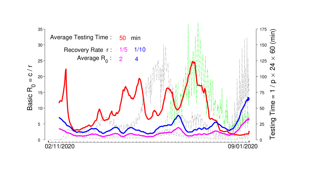
Figure 8: Future Study: A preview to post-mortem analysis on the pandemic. Notice that the basic reproduction number climbed up with the appearance of the omicron variant in the months of July and August, 2021. Background data in green is the daily vaccination numbers in unit of $1.25\times 10^{5}$ in the same plot scale as the data in Fig.3. The $R_{0}$ number is consistent with other’s estimates (e.g. [21]).

Discussion. We can further consolidate the performance of our method to one value for each case total and death total: the median value of their MSRE (Fig.7). That is, we can say the median MSRE error for a 28-day forecasting is 0.0473 (the (+14)-day’s MSRE) for the case total and 0.052 for the death total. By exactly the same definition, the median MSRE error for a 28-day forecasting is 0.395 for the daily cases and 0.3335 for the SDA cases, and, 0.392 for the daily deaths and 0.2481 for the SDA deaths, both are expected to have greater variations than their cumulative totals, which tend to smooth out short-term volatilities. In comparison, a forecaster’s biased coat-tail median MSREs (Fig.4) are smaller than or around half the observer’s values.

There are many ways to make use of the 30 best-fits over the 590-day study period. For example, one can use them as initial guesses to fit their own models to other data, over longer period of time, for real time forecasting, for different states or countries. For another example, one can use them to do post-mortem analyses on the pandemic. Fig.8 shows a preview to such studies. It shows if the average recovery time is 10 days, then on average each infectious person will pass the virus to 4 persons. We intend to publish such a study in the future.

Although the model dynamics of Fig.1 is not meant for the real data, the parameter values are taken from one of the best-fits. It appears to show that the virus can cause an outbreak for 100–200 days. This information on its own may not mean much, but when it is viewed together with the real data over the 590-day study period, it seems to suggest that on average the outbreak caused by each variant does last about 100–200 days. This points to a future modification of our SICM model to include multi-variant dynamics to the model. The insert of Fig.6 is chosen to show such a need. It suggests that one outbreak is ending and another outbreak is starting. Our one-variant SICM model performs poorly during such overlapping periods, in which its projections are trending in the wrong direction. With a two-variant model, such transitions are expected to become smoother, and possibly further reduce the MSREs for the daily and SDA numbers shown in Fig.7.

I did a real-time forecasting for the New York State’s case number from March 20 to April 30, 2020 ([6]). I stopped the experiment when I realized the simple variant of the SIR model I used was not capable to generate the seven-day oscillation. This study is a continuation of that experiment, and our SICM model is an improvement as a result. However, it is meant to be a minimal model capable of the oscillation, and there are room for improvements. For example, because its primary projection consistently under estimate the real data, the model should be further revised to reduce the amount of abberations. One possible modification is to try a Holling Type-II form for the daily infection rate term $cSI$. Another possible improvement is to include the daily test number into the best-fit that includes the number of test-negative individuals from the susceptible group $S$. These modifications may also reduce the MSREs for the daily and SDA numbers.

There is a possible immediate ad hoc addition to our daily forecasting regime that may improve the daily and SDA errors. By comparing the coat-tail daily plot from the insert of Fig.4 and the boosted AAC forecast from the insert of Fig.7, we can see that the latter removes almost all the under-abberations for the SDA numbers but add more over-abberations to the time periods when the cases reach local maximums. Thus, the additional rule is to turn off boosted AAC whenever the SDA exhibits a consecutive overestimate of the data for 3 to 7 days, and then turn on boosted AAC whenever the primary SDA projection becomes an underestimate for a few days in a row.

We note that the testing time $1/p$ shown in Fig.8 by definition is the same as the handling time from mathematical ecology. This time definitely includes the time from the moment when a sample is collected to the moment when the result is entered into the reporting system which generated the data for this study. But it should not include the time taken to inform the patient. It may not include excessive idling time the sample is not processed, which as an assumption may be subject to debate. The last comment before closing is this, the usefulness of the method depends on the data and the model. Bad data or bad model will make the whole exercise pointless.

The methodology we adopted is as traditional as Newtonian mechanics: construct a model for a system, fit the model to real data, and make prediction for the future trajectory of the system. There is not a better example for this Newtonian tradition than the planetary model for the solar system. Obviously, our model for the Covid-19 epidemic is nowhere as good as many models in physics and engineering. Our method for best-fitting follows the same tradition by gradient search, another great idea by Newton. In our case and for all applications of Artificial Intelligence where gradient search is the key, we are simply leveraging the power of computers for an old idea. The similarity between our method and the Newtonian tradition ends here. Because of its accuracy, there is few abberation in the prediction of planetary motion by Newton’s gravitational model, and hence its forecaster’s plot and observer’s plot are the same. In contrast, because of our model’s incompleteness, abberations to projection are bound to happen. This is perhaps the lesson we learn from this paper, and as a result to stimulate others to find better models and to improve the science of epidemiological forecasting so that we can be better prepared for the next pandemic.

Declarations

Ethical approval: Not Applied.

Conflict of interests: None.

Authors’ Contributions: Not Applied.

Funding: None.

Availability of data and materials: All best-fitted data for this article can be downloaded from [7]. Additional materials can be made available from the author on reasonable request.

References

- [1] Anastassopoulou, C., Russo, L., Tsakris, A., & Siettos, C. Data-based analysis, modelling and forecasting of the COVID-19 outbreak. PloS one, 15(3), e0230405 (2020).
- [2] Bertozzi, A.L. et al. The challenges of modeling and forecasting the spread of COVID-19. Proceedings of the National Academy of Sciences, 117(29), 16732–16738 (2020).
- [3] Brauer, F. and Castillo-Chavez, C. Mathematical Models in Population Biology and Epidemiology, Springer Science and Business Media (2013).
- [4] Deng, B. An Inverse Problem: Trappers Drove Hares to Eat Lynx, Acta Biotheor, 66, 213–242 (2018).
- [5] Deng, B. Neuron Model with Conductance-Resistance Symmetry, Physics Letter A, Volume 383, Article 125976 (2019).
- [6] Deng, B. An Empirical Forecasting Method for Epidemic Outbreaks with Application to Covid-19, Mathematics in Applied Sciences and Engineering, 2, 1–71 (2021)
- [7] Deng, B. Data for ‘Forecast U.S. Covid-19 Numbers by Open SIR Model with Testing’. https://doi.org/10.6084/m9.figshare.21968660 (2023)
- [8] CDC. data.cdc.gov/Case-Surveillance/United-States-COVID-19-Cases-and-Deaths-by-State-o/ 9mfq-cb36 (2021).
- [9] Holling, C.S. Some characteristics of simple types of predation and parasitism1. The canadian entomologist, 91(7), 385–398 (1959).
- [10] Ioannidis, J. P., Cripps, S., & Tanner, M. A. Forecasting for COVID-19 has failed. International journal of forecasting, 38(2), 423–438 (2020).
- [11] Lawton, J.H., Beddington, J.R., Bonser, R. Switching in invertebrate predators. In: Usher, M.B., Williamson, M.H. (eds) Ecological stability. Chapman and Hall, London, 141–-158 (1974).
- [12] Logan, J.D., Ledder, G., & Wolesensky, W. Type II functional response for continuous, physiologically structured models. Journal of t heoretical biology, 259(2), 373–381 (2009).
- [13] Luo, J. Forecasting COVID-19 pandemic: Unknown unknowns and predictive monitoring. Technological forecasting and social change, 166, 120602 (2021).
- [14] Moein, S., et al. Inefficiency of SIR models in forecasting COVID-19 epidemic: a case study of Isfahan. Scientific reports, 11(1), 4725 (2021).
- [15] Murdoch, W.W. The functional response of predators. J Appl Ecol. 10, 335-–342 (1973).
- [16] Petropoulos, F., Makridakis, S., & Stylianou, N. COVID-19: Forecasting confirmed cases and deaths with a simple time series model. International journal of forecasting, 38(2), 439–452 (2022).
- [17] Rahimi, I., Chen, F. and Gandomi, A.H. A review on COVID-19 forecasting models. Neural Comput & Applic. https://doi.org/10.1007/s00521-020-05626-8 (2021).
- [18] Ruszczynski, A.P. Nonlinear Optimization, Princeton University Press, Princeton (2006).
- [19] Shinde, G.R., et al. Forecasting models for coronavirus disease (COVID-19): a survey of the state-of-the-art. SN Computer Science, 1, 1–15 (2020).
- [20] Van den Driessche, P. and Watmough, J. Reproduction numbers and sub-threshold endemic equilibria for compartmental models of disease transmission, Mathematical Biosciences, 180, 29–48 (2002).
- [21] Zou, D.,et al. Epidemic model guided machine learning for COVID-19 forecasts in the United States. MedRxiv, doi: https://doi.org/10.1101/2020.05.24.20111989 (2020).