Fuse It or Lose It: Deep Fusion for Multimodal Simulation-Based Inference

Abstract

We present multimodal neural posterior estimation (MultiNPE), a method to integrate heterogeneous data from different sources in simulation-based inference with neural networks. Inspired by advances in attention-based deep fusion learning, it empowers researchers to analyze data from different domains and infer the parameters of complex mathematical models with increased accuracy. We formulate different multimodal fusion approaches for MultiNPE (early, late, and hybrid) and evaluate their performance in three challenging numerical experiments. MultiNPE not only outperforms naïve baselines on a benchmark model, but also achieves superior inference on representative scientific models from neuroscience and cardiology. In addition, we systematically investigate the impact of partially missing data on the different fusion strategies. Across our different experiments, late and hybrid fusion techniques emerge as the methods of choice for practical applications of multimodal simulation-based inference.

1 Introduction

Simulations have become a fundamental tool to model complex phenomena across many domains in science and engineering [33]. High-fidelity simulation programs implement theories by domain experts, and their exact behavior is controlled by parameters $\boldsymbol{\theta}$ and latent program states $\boldsymbol{\xi}$ [13]. Typically, the simulation parameters $\boldsymbol{\theta}$ are unknown and must be inferred from observable data $\mathcal{D}$ to understand the underlying data generating mechanism. The probabilistic (Bayesian) approach to this inverse problem aims to approximate the posterior distribution $p(\boldsymbol{\theta}\,|\,\mathcal{D})\propto p(\boldsymbol{\theta})\,p(\mathcal{D}\,|\,\boldsymbol{\theta})$, given a prior $p(\boldsymbol{\theta})$ and observable data $\mathcal{D}$. While sampling synthetic data from a mechanistic simulator is typically easy, the likelihood $p(\mathcal{D}\,|\,\boldsymbol{\theta})$ is generally only implicitly defined via a high-dimensional integral over all possible execution paths $\boldsymbol{\xi}$ of the simulator, $p(\mathcal{D}\,|\,\boldsymbol{\theta})=\int p(\mathcal{D},\boldsymbol{\xi}\,|\,\boldsymbol{\theta})\mathrm{d}\boldsymbol{\xi}$, which is analytically intractable for complex simulators of practical interest [13]. This intractability disqualifies established Bayesian inference algorithms, such as MCMC [42] or variational inference [7], which rely on the ability to explicitly and repeatedly evaluate the likelihood for any pair $(\boldsymbol{\theta},\mathcal{D})$. In contrast, simulation-based inference (SBI) methods [5, 54] relax this requirement and only require synthetic tuples $(\boldsymbol{\theta},\mathcal{D})$ from the simulation program.

The relatively new family of neural posterior estimation (NPE) algorithms uses a conditional neural density estimator (e.g., normalizing flow; [46]) to learn a surrogate $q_{\boldsymbol{\phi}}(\boldsymbol{\theta}\,|\,\mathcal{D})$ for the posterior $p(\boldsymbol{\theta}\,|\,\mathcal{D})$ in a simulation-based training phase. Subsequently, the upfront training effort is amortized by nearly instant posterior inference: For a new observed data set $\mathcal{D}_{o}$, the neural approximator can instantly sample from the approximate posterior $q_{\boldsymbol{\phi}}(\boldsymbol{\theta}\,|\,\mathcal{D}_{o})$.

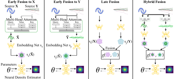
Figure 1: Multimodal neural posterior estimation (MultiNPE) is a family of principled methods to integrate information from multiple heterogeneous data sources $\mathbf{X}$ and $\mathbf{Y}$ in simulation-based inference (SBI). Early fusion to $\mathbf{X}$ uses multi-head attention with $\mathbf{X}$ as query and $\mathbf{Y}$ as both key and value, arriving at the cross-informed $\tilde{\mathbf{X}}$. Equivalently, early fusion to $\mathbf{Y}$ uses $\mathbf{Y}$ as query and yields $\tilde{\mathbf{Y}}$. Both early fusion variants use a neural network $s_{\cdot}({\cdot})$ to learn a representation of the fused data. In contrast, late fusion learns separate embeddings $s_{x}(\mathbf{X})$ and $s_{y}(\mathbf{Y})$, and then fuses the embeddings. Hybrid fusion combines both worlds by using a symmetrical cross-shaped multi-head attention like in early fusion, followed by separate embeddings and a late fusion step. See Section 3 for a more formal specification.

Neural SBI (i.e., NPE and other related algorithms) is still in its infancy, and we extend its repertoire to the practically relevant class of mechanistic multimodal models, where a set of shared parameters influences heterogeneous sources of data via distinct simulators. Relevant examples include computational models in cardiovascular precision medicine [60], or integrative models of decision making and neural activity in the cognitive sciences [24]. SBI currently lacks the tools to properly analyze such multimodal data. Our paper addresses this fundamental limitation of NPE with the following main contributions:

1. We present multimodal neural posterior estimation (MultiNPE), which enables the integration of multimodal data into simulation-based inference methods.

2. We develop variations of MultiNPE, translating advances in attention-based deep fusion learning into probabilistic machine learning with neural networks.

3. We demonstrate that MultiNPE outperforms existing SBI algorithms on a 10-dimensional reference task and two scientific models from neuroscience and cardiology.

2 Preliminaries

This section gives a brief overview of neural posterior estimation, learned summary statistics, and multi-head attention. Acquainted readers can fast-forward to Section 3.

2.1 Neural posterior estimation

The inverse problem of approximating the posterior distribution in SBI can be tackled by targeting the posterior directly with a class of algorithms called neural posterior estimation (NPE; [44, 48, 22, 53, 26]). Other methods approach the problem indirectly by approximating the likelihood [45, 39], the likelihood-to-evidence ratio [29], or the joint distribution [50, 25, 65]. NPE uses a conditional neural density estimator $q_{\boldsymbol{\phi}}(\boldsymbol{\theta}\,|\,\mathcal{D})$ with neural network parameters $\boldsymbol{\phi}$, such as a normalizing flow [46], score-matching networks [22, 53], or flow matching [14]. Here, we focus on normalizing flows due to their fast single-pass inference and simple training, even though our approach for multimodal SBI translates seamlessly to other backbone neural density estimators (see Experiment 3 for flow matching).

A conditional normalizing flow learns a map from a simple base distribution (e.g., a unit Gaussian) to the target posterior $p(\boldsymbol{\theta}\,|\,\mathcal{D})$. The normalizing flow is optimized by minimizing the Kullback-Leibler (KL) divergence between the true posterior $p(\boldsymbol{\theta}\,|\,\mathcal{D})$ and its approximation $q_{\boldsymbol{\phi}}(\boldsymbol{\theta}\,|\,\mathcal{D})$ via the maximum likelihood objective $\mathbb{E}_{p(\boldsymbol{\theta})\,p(\mathcal{D}\,|\,\boldsymbol{\theta})}\big{[}-\log q_{\boldsymbol{\phi}}(\boldsymbol{\theta}\,|\,\mathcal{D})\big{]}$. The normalizing flow can be trained on samples $(\boldsymbol{\theta},\mathcal{D})$ from the joint distribution $p(\boldsymbol{\theta},\mathcal{D})=p(\boldsymbol{\theta})\,p(\mathcal{D}\,|\,\boldsymbol{\theta})$, which is equivalent to generating data by the simulation programs in SBI. Crucially, once the normalizing flow has been trained, it can evaluate and sample from the posterior density $q_{\boldsymbol{\phi}}(\boldsymbol{\theta}\,|\,\mathcal{D}_{o})$ for new observed data $\mathcal{D}_{o}$ with a single pass through the trained neural density estimator. By recasting costly probabilistic inference as a neural network prediction task, normalizing flows achieve amortized inference across the joint distribution $p(\boldsymbol{\theta},\mathcal{D})$.

2.2 Embedding networks for end-to-end learned summary statistics

In Bayesian inference, the data $\mathcal{D}$ can be replaced by sufficient summary statistics $s_{*}(\mathcal{D})$ without altering the posterior: $p(\boldsymbol{\theta}\,|\,\mathcal{D})=p(\boldsymbol{\theta}\,|\,s_{*}(\mathcal{D}))$. Ideally, $s_{*}$ is also low-dimensional, achieving lossless compression with regard to $\boldsymbol{\theta}$ conditional on $\mathcal{D}$. While low-dimensional sufficient summary statistics are notoriously difficult to find for complex problems, the task of constructing approximate summary statistics $s(\mathcal{D})$ with $p(\boldsymbol{\theta}\,|\,\mathcal{D})\approx p(\boldsymbol{\theta}\,|\,s(\mathcal{D}))$ has been extensively studied for approximate Bayesian inference. Within neural SBI, neural networks are employed to learn embeddings of the data $\mathcal{D}$ in tandem with the posterior approximator [66, 48, 49, 12, 64, 10, 31]. These embedding networks $s_{\boldsymbol{\psi}}$ learn a transformation that aims to obtain low-dimensional sufficient statistics of the data $\mathcal{D}$, parameterized by learnable neural network weights $\boldsymbol{\psi}$. The NPE loss with learned embeddings $s_{\boldsymbol{\psi}}(\mathcal{D})$ minimizes the objective

$$\mathcal{L}(\boldsymbol{\phi},\boldsymbol{\psi})=\mathbb{E}_{p(\boldsymbol{\theta})\,p(\mathcal{D}\,|\,\boldsymbol{\theta})}\big{[}-\log q_{\boldsymbol{\phi}}\big{(}\boldsymbol{\theta}\,|\,s_{\boldsymbol{\psi}}(\mathcal{D})\big{)}\big{]},$$ (1)

and we shall omit the embedding network weights $\boldsymbol{\psi}$ for brevity. The concrete architecture of the embedding network $s(\cdot)$ should match the probabilistic symmetries of the data. For example, $i.i.d.$ data sets can be embedded with a permutation-invariant neural network, such as a DeepSet [69] or an attention-based set transformer [34]. Similarly, time series data require a neural architecture which respects their probabilistic structure in time, such as an LSTM [30] or an attention-based temporal fusion transformer [62].

2.3 Multi-head attention

Attention mechanisms play a crucial role in machine learning, and one of the most notable architectures that has revolutionized the field is the Transformer [57]. The Transformer introduces a highly effective mechanism for capturing dependencies and relationships within sequences of data, making it particularly well-suited for tasks such as natural language processing [57] or computer vision [16]. The core of the Transformer’s attention mechanism is the scaled dot-product attention, which is defined as

$$\mathrm{Attention}(Q,V,K)=\mathrm{softmax}\left(\dfrac{QK^{\top}}{\sqrt{d_{k}}}\right)V,$$ (2)

with queries $Q$, values $V$, and keys $K$ of dimension $d_{K}$. To enhance the model’s ability to capture different types of relationships and dependencies in the data, the Transformer employs multi-head attention (MHA). MHA enables the model to jointly attend to information from different subspaces of the data across multiple attention heads. Each attention head is a separate instance of the scaled dot-product attention mechanism (Equation 2), and their outputs are combined using learnable linear transformations to produce the final multi-head attention output,

$$\mathrm{MHA}(Q,V,K) =\big{[}\mathrm{head}_{1},\ldots,\mathrm{head}_{h}\big{]}W^{O}$$ (3)

$$\mathrm{head}_{i} =\mathrm{Attention}(QW_{i}^{Q},KW_{i}^{K},VW_{i}^{V})$$

where $h$ represents the number of attention heads, and $W^{O}$, $W_{i}^{Q}$, $W_{i}^{K},W_{i}^{V}$ are learnable weight matrices for combining the outputs of individual attention heads. The multi-head attention mechanism allows the Transformer model to encode patterns and relationships in the data, making it highly effective for a range of sequence-to-sequence tasks.

3 Method

3.1 Simulation paradigm and notation

In this section, we consider multimodal test data $\mathcal{D}_{o}=\{\mathbf{X}_{o},\mathbf{Y}_{o}\}$ from two sources, as well as a simulation program capable of generating synthetic data $\mathcal{D}=\{\mathbf{X},\mathbf{Y}\}$. An instance of either data source can consist of multiple observations, e.g. patients in a medical trial, or discrete steps in a time series. We use $N$ for the cardinality of the first source, $\mathbf{X}\equiv\{\mathbf{x}_{n}\}_{n=1}^{N}$, and $M$ for the cardinality of the second source $\mathbf{Y}\equiv\{\mathbf{y}_{m}\}_{m=1}^{M}$. Following the standard notation in SBI, the neural networks are trained on a total of $K$ data sets $\{\mathcal{D}^{(k)}\}_{k=1}^{K}\equiv\{\{\mathbf{X}^{(k)},\mathbf{Y}^{(k)}\}\}_{k=1}^{K}$. $K$ is also called the simulation budget. To shorten notation, we drop the data set index $k$ when it is not relevant to the context. The sub-programs generating the individual data modalities are based on common parameters $\boldsymbol{\theta}$ as well as domain-specific parameters $\boldsymbol{\theta}_{x},\boldsymbol{\theta}_{y}$. Using the verbose notation once to avoid ambiguity, the joint forward model $p(\boldsymbol{\theta},\boldsymbol{\theta}_{x},\boldsymbol{\theta}_{y},\mathbf{X},\mathbf{Y})$ for a single data set $\mathcal{D}^{(k)}=\{\mathbf{X}^{(k)},\mathbf{Y}^{(k)}\}$ is defined as:

$$\boldsymbol{\theta}^{(k)},\boldsymbol{\theta}_{x}^{(k)},\boldsymbol{\theta}_{y}^{(k)} \sim p(\boldsymbol{\theta},\boldsymbol{\theta}_{x},\boldsymbol{\theta}_{y})$$ (4)

$$\mathbf{x}_{n}^{(k)} \sim p(\mathbf{x}\,|\,\boldsymbol{\theta}^{(k)},\boldsymbol{\theta}_{x}^{(k)}),\;\;n=1,\ldots,N$$

$$\mathbf{y}_{m}^{(k)} \sim p(\mathbf{y}\,|\,\boldsymbol{\theta}^{(k)},\boldsymbol{\theta}_{y}^{(k)}),\;\;m=1,\ldots,M$$

The result of sampling from this forward model $K$ times is a set of $K$ tuples of parameters and data sets,

$$\Big{\{}\underbrace{\big{\{}\boldsymbol{\theta}^{(k)},\boldsymbol{\theta}_{x}^{(k)},\boldsymbol{\theta}_{y}^{(k)}\big{\}}}_{\text{Parameters}},\underbrace{\big{\{}\mathbf{X}^{(k)},\mathbf{Y}^{(k)}\big{\}}}_{\text{Data}\;\mathcal{D}^{(k)}}\Big{\}}_{k=1}^{K},$$

and the inverse problem consists in inferring all unknown parameters from the data. Because SBI uses a synthetic simulation program, the ground-truth parameter values are available during the training phase. In the inference (test) phase however, the ground truth parameters of the test data $\mathcal{D}_{o}=\{\mathbf{X}_{o},\mathbf{Y}_{o}\}$ are naturally unknown and need to be estimated by the generative network $q_{\boldsymbol{\phi}}(\boldsymbol{\theta},\boldsymbol{\theta}_{x},\boldsymbol{\theta}_{y}\,|\,\mathbf{X},\mathbf{Y})$.

3.2 Necessity of principled deep fusion

Consider the scenario where we estimate a single shared parameter $\boldsymbol{\theta}$ that manifests itself in both an $i.i.d.$ data set $\mathbf{X}\sim p(\mathbf{X}\,|\,\boldsymbol{\theta})$ and a Markovian time series $\mathbf{Y}\sim p(\mathbf{Y}\,|\,\boldsymbol{\theta})$. The fundamentally different probabilistic systems for $\mathbf{X}$ and $\mathbf{Y}$ cannot possibly be efficiently learned with a single neural architecture because (i) a permutation invariant network is suited for $i.i.d.$ data but cannot capture the autoregressive structure of a time series; and (ii) a time series network can fit time series but cannot efficiently learn the permutation-invariant structure of $i.i.d.$ data. As a consequence, we need separate information processing streams to accommodate the specific structure of each data source. Yet, the neural density estimator $q_{\boldsymbol{\phi}}$ demands a fixed-length conditioning vector $s(\mathcal{D})$. We serve both requirements simultaneously: First, we process the heterogeneous streams of information $\mathbf{X}$ and $\mathbf{Y}$ with dedicated architectures. Second, we integrate the information into a fixed-length embedding before it enters the neural density estimator.

When either of the simulators has no individual parameters, we revert to a special case of Equation 4 and our method remains unaltered (see Experiments 1 and 3). However, if there are no shared parameters, a multimodal architecture will clearly not have any advantage over separate NPE algorithms for the two sub-problems.

3.3 Fusion strategies

The integration of information from different data sources is called fusion, and there are multitudes of options for how and when the fusion happens (see Figure 1). Previous work on deep fusion learning differentiates early fusion, late fusion, and hybrid approaches [4, 27, 70].

Early fusion performs the fusion step as early as possible, ideally directly on the raw data (see Figure 1 panel 1 and 2). We implement this via cross-attention [38, 41] between the input modalities $\mathbf{X}$ and $\mathbf{Y}$. Concretely, we use multi-head attention [57] with queries $Q$, values $V$, and keys $K$. The data inputs $\mathbf{X}$ and $\mathbf{Y}$ can differ with respect to their dimensions but the shapes of $V$ and $K$ must align for multi-head attention. Thus, we select one of the data sources ($\mathbf{X}$ or $\mathbf{Y}$) as query $Q$ while the other one acts as both value $V$ and key $K$. In Experiment 1, we illustrate that the choice of data sources for $Q$ and $V,K$ influences the results when the data sources $\mathbf{X}$ and $\mathbf{Y}$ differ with respect to their informativeness. After the attention-based fusion step, we pass the output of the multi-head attention block to a suitable embedding network $s_{\cdot}(\cdot)$ to provide a proper input for the conditional neural density estimator $q_{\boldsymbol{\phi}}$. In summary, the information flow in early fusion is

$$s(\mathcal{D})=\begin{cases}s_{x}\Big{(}\mathrm{MHA}\big{(}Q(\mathbf{X}),V(\mathbf{Y}),K(\mathbf{X})\big{)}\Big{)}\hskip 2.84544pt\leftarrow\text{E.\,F. to}\ \mathbf{X}\\ s_{y}\Big{(}\mathrm{MHA}\big{(}Q(\mathbf{Y}),V(\mathbf{X}),K(\mathbf{X})\big{)}\Big{)}\hskip 2.84544pt\leftarrow\text{E.\,F. to}\ \mathbf{Y}\\ \end{cases}$$ (5)

where $\mathrm{MHA}(Q,V,K)$ denotes multi-head attention (see Section 2.3) and E. F. is an abbreviation for early fusion.

Late fusion is a diametrical approach where the fusion step happens at a later stage (see Figure 1 panel 3). In SBI with learnable embeddings, this translates to fusion immediately before passing the final embedding to the conditional neural density estimator as conditioning variables. At this stage, both data inputs have already been embedded into learned summary statistics $s_{x}(\mathbf{X})$ and $s_{y}(\mathbf{Y})$ with fixed lengths each. Thus, late fusion can be achieved by simply concatenating the embeddings, $s(\mathcal{D})=g\big{(}s_{x}(\mathbf{X}),s_{y}(\mathbf{Y})\big{)}=\big{[}s_{x}(\mathbf{X}),s_{y}(\mathbf{Y})\big{]}$, which is a common choice for the fusion function $g$ [4, 27, 70].

Hybrid fusion combines components from both early and late fusion (see Figure 1 panel 4). Initially, we use cross attention with both $\mathbf{X}$ and $\mathbf{Y}$ as the query $Q$. In particular, we construct a cross-shaped information flow where we embed each data source using cross-attention information from the other source. This leads to a symmetrical information flow and overcomes the drawback of early fusion, where one of the data sources must be chosen as the query $Q$. The outputs of the symmetrical cross-attention step are then each passed an embedding network $s_{x}(\cdot),s_{y}(\cdot)$, and the information streams are fused just before entering the neural density estimator:

$$\tilde{\mathbf{X}} =\mathrm{MHA}\big{(}Q(\mathbf{X}),V(\mathbf{Y}),K(\mathbf{Y})\big{)}$$ (6)

$$\tilde{\mathbf{Y}} =\mathrm{MHA}\big{(}Q(\mathbf{Y}),V(\mathbf{X}),K(\mathbf{X})\big{)}$$

$$s(\mathcal{D}) =g\big{(}s_{x}(\tilde{\mathbf{X}}),s_{y}(\tilde{\mathbf{Y}})\big{)}=\big{[}s_{x}(\tilde{\mathbf{X}}),s_{y}(\tilde{\mathbf{Y}})\big{]}$$

We hypothesize that hybrid fusion enables more flexible resource allocation: Features of an informative source as well as interactions can be captured in the embedding network, which reduces the burden on the generative network $q_{\boldsymbol{\phi}}$.

3.4 More than two data sources

This section will discuss the natural extension of our fusion architectures beyond two sources. In the following, let $L\in\mathbb{N}_{\geq 2}$ be the number of data sources $\mathcal{D}=\{\mathcal{D}_{l}\}_{l=1}^{L}$.

Late fusion naturally translates to an arbitrary number of sources: Each source $\mathcal{D}_{l}$ has a dedicated embedding network $s_{l}(\mathcal{D}_{l})$ to learn sufficient summary statistics for posterior inference. Finally, all embeddings are combined into a joint embedding $s(\mathcal{D})=g\big{(}s_{1}(\mathcal{D}_{1}),\ldots,s_{L}(\mathcal{D}_{L})\big{)}$ with suitable $g$ (e.g., concatenation as above). Thus, the number of networks in late fusion scales linearly in $\mathcal{O}(L)$. Early and hybrid fusion, however, involve pairwise cross-attention blocks, which do not natively generalize to $L\geq 2$ inputs. For early fusion, there are $L!$ options to choose the layout of pairwise cross-attention fusion blocks, but only $1+\ldots+(L-1)$ blocks must be realized in practice to implement a cascade of cross-attention steps for early fusion. In addition, we require one embedding network, leading to a total of $1+2+\ldots+(L-1)+1\in\mathcal{O}(L^{2})$ networks. In hybrid fusion, however, we want a full cross-exchange of information across all sources, which requires a total of $L!$ networks. In addition, each source needs one embedding network. This leads to a total of $L!+L\in\mathcal{O}(L!)$ networks, which clearly raises scaling issues for large $L$. Thus, a central question of this paper is to assess the extent to which the scalable late fusion approach yields similar results to the more computationally complex hybrid fusion method.

3.5 Hardships of neural network training

Introducing multi-head attention blocks (early & hybrid fusion) or multiple embedding networks (late & hybrid fusion) increases the complexity of the neural architecture and thereby increases the risk of undesirable artifacts such as overfitting or vanishing gradients. This necessitates modern training techniques from deep learning (see Empirical evaluation), such as weight regularization [37], learning rate schedules [68], and dropout layers [55], which are seldomly discussed explicitly in the SBI literature.

4 Related work

Multimodal fusion.

Researchers have long been integrating different types of features to improve the performance of machine learning applications [43]. As [28] remark, using deep fusion to learn fused representations of heterogeneous features in multimodal settings is a natural extension of this strategy. Recently, attention-based transformer networks have been employed for multimodal problems across many applications [67], such as image and sentence matching [61], multispectral object detection [47], or integration of image and depth information [21]. We confirm the potential of cross-attention architectures in probabilistic machine learning with conditional neural density estimators. All of our fusion strategies implement a unified embedding for heterogeneous data sources, which is an instantiation of the joint representation archetype in the taxonomy of [28].

Multimodality and missing data.

Multimodal learning algorithms can naturally address the problem of missing data because missing information from one source may be compensated for by another source (see Experiment 2). In the context of multimodal time series, this issue has been addressed by factorized inference on state space models [71] and learned representations via tensor rank regularization [35]. While our multimodal NPE method also learns robust representations from partially missing data, we use fusion techniques that respect the probabilistic symmetry of the data, rather than a certain factorization of the posterior distribution. From a general angle, Bayesian meta-learning [20] has been used to study the efficiency of multimodal learning under missing data, both during training and inference time [40]. Similarly, our approach embodies principles of Bayesian meta-learning by extending the amortization scope of NPE to varying degrees of missingness, which is in turn facilitated by our multimodal fusion schemes.

Hierarchical Bayesian models.

Hierarchical or multilevel Bayesian models [23] are used to model the dependencies in nested data, where observations are organized into clusters or levels. While these models often feature shared parameters across observational units or global parameters describing between-cluster variations [63], they focus on analyzing the variations of a single data modality at different levels. In contrast, multimodal models capitalize on integrating information from different sources or modalities. That being said, a multimodal problem could also be formulated in a hierarchical way, such that the shared parameters of different modalities admit a hierarchical prior. And while the complexity of such models quickly becomes prohibitive, our MultiNPE approach could pave the way for hierarchical multimodal approaches where the latter have been foregone merely out of computational desperation.

Learned summary embeddings.

The task of learning low-dimensional embeddings of data has been extensively studied under different names, such as representations [6], features [52], embeddings [2], or summary statistics [8]. In the context of approximate Bayesian computation [19], using a function to compress potentially high-dimensional data into low-dimensional summary statistics is paramount to the applicability of posterior approximation algorithms. Moreover, many neural approaches to SBI have explicitly focused on learning approximately sufficient statistics end-to-end with neural approximators [66, 48, 49, 12, 64, 10], for integration with downstream samplers [32], or in a fully unsupervised manner [18, 1]. None of these methods have explored learning multimodal representations for SBI.

5 Empirical evaluation

Settings.

We evaluate MultiNPE in a synthetic multimodal model with fully overlapping parameter spaces across the data modalities, a neurocognitive model with partially overlapping parameter spaces and missing data, and a cardiovascular data set with three data sources.

Evaluation metrics.

For all experiments, we evaluate the accuracy of the posterior estimates as well as their uncertainty calibration and Bayesian information gain on $J$ unseen test data sets $\{\mathcal{D}^{(j)}_{o}\}_{j=1}^{J}$ with known ground-truth parameters $\{\boldsymbol{\theta}^{(j)}_{*}\}_{j=1}^{J}$. Let $\{\boldsymbol{\theta}^{(j)}_{s}\}_{s=1}^{S}$ be the set of $S$ posterior draws from the neural approximator $q_{\boldsymbol{\phi}}(\boldsymbol{\theta}\,|\,\mathcal{D}_{o}^{(j)})$ conditioned on the data set $\mathcal{D}_{o}^{(j)}$. For accuracy, we compute the average root mean square error (RMSE) between posterior means and ground truth parameter values over the test set:

$$\mathrm{RMSE}=\frac{1}{J}\sum_{j=1}^{J}\sqrt{\frac{1}{S}\sum_{s=1}^{S}\big{(}\boldsymbol{\theta}^{(j)}_{s}-\boldsymbol{\theta}_{*}^{(j)}\big{)}^{2}}$$ (7)

We quantify uncertainty calibration via simulation-based calibration (SBC; [56]): For the true posterior $p(\boldsymbol{\theta}\,|\,\mathcal{D})$, all uncertainty regions $U_{q}(\boldsymbol{\theta}\,|\,\mathcal{D})$ of the posterior are well calibrated for any quantile $q\in(0,1)$ [9], that is:

$$q=\iint\mathbf{I}[\boldsymbol{\theta}_{*}\in U_{q}(\boldsymbol{\theta}\,|\,\mathcal{D})]\,p(\mathcal{D}\,|\,\boldsymbol{\theta}_{*})\,p(\boldsymbol{\theta}_{*})\mathrm{d}\boldsymbol{\theta}_{*}\mathrm{d}\mathcal{D},$$ (8)

where $\mathbf{I}[\cdot]$ is the indicator function. Discrepancies from this equality indicate insufficient calibration of an approximate posterior. We report the median SBC error of central credible intervals computed for 20 linearly spaced quantiles $q\in[0.5\%,99.5\%]$, averaged across the test data set (aka. expected calibration error; ECE). Finally, we quantify the (Bayesian) information gain via posterior contraction, based on the relation between prior and posterior variance, $1-\operatorname{Var}(\mathrm{Prior})/\operatorname{Var}(\mathrm{Posterior})$, averaged across test data sets. All three metrics are global in the sense that they estimate performance across the entire joint model $p(\boldsymbol{\theta},\mathcal{D})$ instead of singling out particular data sets or true model parameters [9]. The metrics can directly be computed based on simulations from the joint model, which is essentially instantaneous due to amortized inference.

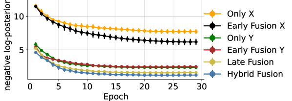
Figure 2: Experiment 1: Two of our multimodal schemes (late fusion and hybrid fusion) outperform single-source architectures (only $\mathbf{X}$/$\mathbf{Y}$), as indexed by better (lower) negative log posterior on held-out validation data across ten training runs.

5.1 Exchangeable data and Brownian time series

This experiment compares MultiNPE and standard NPE on a synthetic task where a common parameter $\boldsymbol{\theta}\in\mathbb{R}^{10}$ is used as (i) the location parameter of Gaussian $i.i.d.$ data $\mathbf{X}$ and (ii) the drift rate of a stochastic trajectory $\mathbf{Y}$,

$$\boldsymbol{\theta}\sim \ \mathrm{Normal}(\boldsymbol{\theta}\,|\,\boldsymbol{0},\boldsymbol{1}),$$ (9)

$$\mathbf{x}_{n}\sim \ \mathrm{Normal}(\mathbf{x}\,|\,\boldsymbol{\theta},\boldsymbol{1}),\;n=1\ldots,N$$

$$\mathrm{d}\mathbf{y}_{m}(t)= \ \boldsymbol{\theta}\,\mathrm{d}t+\sigma\,\mathrm{d}\mathbf{W}(t),\;m=1,\ldots,M$$

$$\ \text{with}\,\mathbf{W}(t)\sim\mathrm{Normal}(\mathbf{W}\,|\,\boldsymbol{0},\boldsymbol{1}),$$

where the $i.i.d.$ data consist of $N=5$ observations $\mathbf{X}=\{\mathbf{x}_{1},\ldots,\mathbf{x}_{5}\}$, the trajectory is discretized into $M=20$ steps $\mathbf{Y}=(\mathbf{y}_{1},\ldots,\mathbf{y}_{20})$ with noise $\sigma=0.5$, an interval of $t=[0,3]$, and the initial condition is $\mathbf{y}_{1}=\boldsymbol{0}$.

We compare the following neural approximators: NPE with input $\mathbf{X}$, NPE with input $\mathbf{Y}$, as well as MultiNPE variants with early fusion to $\mathbf{X}$, early fusion to $\mathbf{Y}$, late fusion, and hybrid fusion. Each neural approximator is trained on the same training set with a simulation budget of $K=5000$ for 30 epochs. All data originating from the $i.i.d.$ source ($\mathbf{X}$ or $\tilde{\mathbf{X}}$) are embedded with a set transformer [34], and data on the time series stream ($\mathbf{Y}$ or $\tilde{\mathbf{Y}}$) are embedded with a temporal fusion transformer [62]. Neural network details (layers, dropout, etc.) are provided in the Appendix.

Architecture	Time${}^{1}\downarrow$	RMSE $\downarrow$	ECE [%] $\downarrow$	Contraction $\uparrow$
Only $\mathbf{X}$	117	0.81	1.43	0.68
	(110, 149)	(0.80, 0.89)	(0.98, 1.84)	(0.61, 0.68)
Only $\mathbf{Y}$	100	0.40	3.44	0.93
	(95, 141)	(0.40, 0.40)	(3.02, 3.63)	(0.93, 0.93)
Early Fusion $\mathbf{X}$	140	0.88	1.35	0.61
	(131, 150)	(0.82, 0.93)	(1.04, 1.80)	(0.57, 0.66)
Early Fusion $\mathbf{Y}$	128	0.45	5.45	0.91
	(118, 152)	(0.45, 0.45)	(5.06, 5.91)	(0.91, 0.91)
Late Fusion	193	0.36	4.73	0.94
	(172, 235)	(0.36, 0.36)	(4.31, 5.21)	(0.94, 0.94)
Hybrid Fusion	227	0.35	4.99	0.95
	(211, 280)	(0.35, 0.35)	(4.44, 5.18)	(0.95, 0.95)

Table 1: Experiment 1: Our multimodal NPE architecture is superior to single-source NPE algorithms on $1\,000$ unseen data sets, as indexed by improved accuracy (RMSE) and information gain (contraction). The subpar calibration under $\mathbf{Y}$ propagates into the fused posteriors. The table shows median (min, max) across ten training runs of each architecture. ¹ Training time [seconds]

Results.

Late fusion and hybrid fusion outperform standard NPE architectures which only have access to a single data source (see Figure 2 and Table 1). It is evident that $\mathbf{X}$ is less informative for the posterior than $\mathbf{Y}$ (“only $\mathbf{X}$” performs much worse than “only $\mathbf{Y}$”). As a consequence, early fusion to $\mathbf{X}$ leads to worse performance than early fusion to $\mathbf{Y}$. We conclude that the efficacy of early fusion depends on the informativeness of the data source used as a query, which is a hyperparameter design choice that we would ideally like to circumvent. In fact, neither late nor hybrid fusion require such a design choice, and both schemes outperform early fusion in this experiment at the cost of longer neural network training. The most expressive neural architecture, hybrid fusion, shows the best performance in this experiment by a small margin. Heuristically, it combines the best of both worlds: Hybrid fusion extracts information from the raw data by the X-shaped cross-attention modules but avoids the necessity of choosing one of the domains to early-fuse into. Yet, the performance advantage over late fusion is small; thus late fusion might be employed in scenarios where practical considerations (e.g., many sources, limited training time) prohibit a hybrid approach.

5.2 Neurocognitive model of decision making and EEG with missing data

This experiment uses a multimodal neurocognitive model that integrates both a cognitive drift-diffusion model for decision making and a representation of the neurological centroparietal positives (CPP) waveforms on an EEG (model 7 from [24]). A drift-diffusion model (DDM; [51]) describes a human’s decision and reaction time as a stochastic evidence accumulation process with explainable parameters [for a detailed description, see 58]. In contrast to the behavioral reaction time data of the DDM, the CPP waveform is a neural marker that is associated with human decision making [24]. In this setting, we study the potential of MultiNPE to tackle (i) partially overlapping parameter spaces; and (ii) missing data. The forward model is parameterized by six parameters (defined below) that govern two partially entangled data generating processes on a trial-by-trial level,

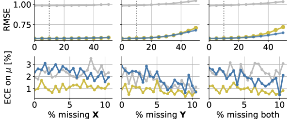
Figure 3: Experiment 2: Hybrid fusion and late fusion consistently show better accuracy (RMSE averaged over all parameters) than the default (direct concatenation). Recall that the training uses 10% missing data (top row, dotted line) and missingness beyond $10\%$ is a substantial extrapolation. Calibration (ECE) of the shared parameter $\mu$ does not clearly differ between the methods.

$$\mu,\sigma,\alpha,\tau,\beta,\eta \sim p(\mu,\sigma,\alpha,\tau,\beta,\eta)\hskip 71.13188pt\text{(prior)}$$ (10)

$$v_{n} \sim\mathrm{Normal}(v\,|\,\mu,\sigma)\hskip 5.69046pt\text{(per-trial entanglement)}$$

$$\mathbf{x}_{n} \sim\mathrm{DDM}(\mathbf{x}\,|\,\alpha,\tau,v_{n},\beta)\hskip 24.18501pt\text{(reaction time)}$$

$$\mathbf{y}_{n} \sim\mathrm{Normal}(\mathbf{y}\,|\,v_{n},\eta)\hskip 29.87547pt\text{(CPP waveform)}$$

with shared global information uptake rate $\mu$ and associated error $\sigma$.

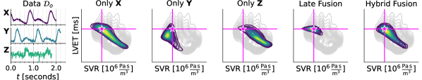
Figure 4: Experiment 3: Bivariate posterior plots of SVR and LVET for one unseen data set $\mathcal{D}_{o}$ (left), as obtained by NPE with affine flows. We show the implicit prior density (gray), the ground-truth $\boldsymbol{\theta}_{*}$ (magenta), and a KDE over 10 000 approximate posterior samples (viridis68,1,8453,183,121). Posteriors from late fusion and hybrid fusion are more concentrated at the ground-truth compared to the single-source methods.

In this model, $\mathrm{DDM}(\mathbf{x}\,|\,\cdot)$ is a drift-diffusion model [58]. Further, $\mathrm{Normal}(\mathbf{y}\,|\,\cdot)$ represents the neurocognitive CPP model from [24]. Crucially, the data sources are entangled on the trial level since the shared information uptake rate $v_{n}$ is sampled for each experimental trial $n$. This implies an equal number of observations for both sources, corresponding to the number of trials, $N{=}M{=}200$, per data set $\mathcal{D}^{(k)}=\{\mathbf{X}^{(k)},\mathbf{Y}^{(k)}\}$. To synthetically induce missing data, we uniformly sample missing rates between $1\%$ and $10\%$ for each training batch and encode missingness as in [59]. With a simulation budget of $K{=}1024$, we compare direct concatenation (default), late fusion, and hybrid fusion.

Results.

As displayed in Figure 3, both late fusion and hybrid fusion outperform direct concatenation via increased accuracy (RMSE) across all missing data rates. The calibration (ECE) on the shared information uptake parameter $\mu$ does not differ between the methods. This underscores the potential of deep fusion in SBI even in situations where the fusion architectures do not have access to more raw data because the naïve approach (i.e., direct concatenation) is possible due to compatible input shapes of the data sources. We hypothesize that our fusion scheme embodies a favorable inductive bias by separating the data sources.

Architecture		Time${}^{1}\downarrow$	RMSE $\downarrow$	ECE [%] $\downarrow$	Contraction $\uparrow$
Affine Flow	Only $\mathbf{X}$	$1296$	$0.94$	$1.90$	$0.53$
	Only $\mathbf{Y}$	$1307$	$1.05$	$1.38$	$0.39$
	Only $\mathbf{Z}$	$1202$	$0.90$	$3.47$	$0.55$
	Late Fusion	$2010$	$0.45$	$5.25$	$0.90$
	Hybrid Fusion	$2761$	$0.75$	$1.33$	$0.68$
Spline Flow	Only $\mathbf{X}$	$1991$	$1.08$	$1.27$	$0.37$
	Only $\mathbf{Y}$	$2028$	$1.05$	$0.82$	$0.39$
	Only $\mathbf{Z}$	$1993$	$1.18$	$0.97$	$0.24$
	Late Fusion	$1880$	$0.87$	0.67	$0.56$
	Hybrid Fusion	$3612$	$0.64$	$1.62$	$0.75$
Flow Matching	Only $\mathbf{X}$	$1040$	$0.55$	$6.93$	$0.85$
	Only $\mathbf{Y}$	$1155$	$0.67$	$6.29$	$0.78$
	Only $\mathbf{Z}$	$993$	$0.83$	$8.30$	$0.72$
	Late Fusion	$2668$	$0.50$	$8.24$	$0.87$
	Hybrid Fusion	$4208$	$0.62$	$5.98$	$0.81$

Table 2: Experiment 3: Test set performance of different generative models (affine flow, spline flow, flow matching) and fusion strategies (single sources, late fusion, hybrid fusion). Taking all three metrics into account, affine flows with late fusion or hybrid fusion yield the best results. ¹ Training time [seconds].

5.3 Cardiovascular in-silico model with 3 sources

Preventing cardiovascular diseases is a fundamental challenge of precision medicine, and scientific hemodynamics simulators are a key to understanding the cardiovascular system [3]. The pulse wave database [11] contains data from 4374 in-silico subjects, validated with in-vivo data. A whole-body simulator models the hemodynamics of the 116 largest human arteries via differential equations and contains measurements of a single heart beat at different locations in the human body, including both photoplethysmograms (PPG) and arterial pressure waveform (APW). Data from the pulse wave database has been previously analyzed with unimodal SBI methods [60], and our experiment is closely inspired by this work. We consider the following measurements as individual data sources $\mathcal{D}=\{\mathbf{X},\mathbf{Y},\mathbf{Z}\}$: PPG at the digital artery ($\mathbf{X}$), PPG at the radial artery ($\mathbf{Y}$), and APW at the radial artery ($\mathbf{Z}$). The shared parameters $\boldsymbol{\theta}$ in this experiment consist of the left ventricular ejection time (LVET), the systemic vascular resistance (SVR), the average diameter of arteries, and the pulse wave velocity.

As an extension to [60], we employ the challenging and realistic setting where measurements from different devices ($\mathbf{X},\mathbf{Y},\mathbf{Z}$) are not synchronized in time (see Figure 4, left, for an example). Concretely, we achieve this with a two-step process: First, we loop the single-beat signals to a longer sequence and crop the sequence into a fixed-length measurement interval for each subject. The length of the cropped signal differs between the sources ($\mathbf{X}$: 2.0 seconds, $\mathbf{Y}$: 2.2 seconds, $\mathbf{Z}$: 1.8 seconds). The sequence onset times are randomly sampled for each subject and source, which means that the cropped signals are not synchronized anymore within each subject. Second, we add Gaussian white noise to the signals, and the signal-to-noise (SNR) ratio is specific for each data source ($\mathbf{X}$: 25dB, $\mathbf{Y}$: 20dB, $\mathbf{Z}$: 30dB). This emulates different measurement devices in a hospital, where each device has a specific measurement error. In this realistic setting, we cannot simply concatenate the inputs, but instead require fusion schemes to integrate the heterogeneous cardiovascular measurements $\mathbf{X},\mathbf{Y},\mathbf{Z}$.

Since the data are only available as an offline data set and not as a simulation program, we face a scenario with both an implicit likelihood and an implicit prior. Further, a subject’s age is a key factor for cardiovascular health in the pulse wave database [11]. Thus, we follow the procedure of [60] and use age as an additional direct condition (i.e., without embedding) for the neural density estimator. We compare the performance of single-source models (i.e., only access to $\mathbf{X}$, $\mathbf{Y}$, or $\mathbf{Z}$) to our multimodal variants late fusion and hybrid fusion. Since simulation-based posterior estimation for this data set is a challenging problem by itself, we further employ each strategy with three different generative models as backbones: (i) affine flows [15]; (ii) neural spline flows [17]; and (iii) flow matching [36].

Results.

Overall, affine flows emerge as the best generative model in this experiment, closely followed by flow matching (see Table 2). The subpar performance of spline flows may be related to the relatively large data dimension in conjunction with the probabilistic geometry of the noisy time series data. Within both affine flows and flow matching, late fusion shows the best combination of high accuracy and information gain, but suffers from poor calibration. As opposed to Experiment 1, late fusion and hybrid fusion differ with respect to their performance profile: While late fusion yields superior accuracy and contraction, it does not reach the calibration quality of hybrid fusion. Thus, we conclude that affine flows with either late fusion or hybrid fusion are desirable in this application from precision medicine, and both fusion schemes have a raison d’être in challenging real-life scenarios. Finally, we illustrate the bivariate posterior of a parameter subspace of practical interest, namely that of SVR and LVET [60], under different fusion schemes in Figure 4. Given one unseen data set $\mathcal{D}_{o}$ and an affine flow backbone, the approximate posteriors of our deep fusion schemes concentrate around the true parameter value $\boldsymbol{\theta}_{*}$ more strongly than single-source NPE. The Appendix contains bivariate posteriors of all generative models and more unseen data sets.

6 Conclusion

In this paper, we presented MultiNPE, a new multimodal approach to perform simulation-based Bayesian inference for models with heterogeneous data generating processes. We achieved this by constructing expressive embedding architectures which are inspired by state-of-the-art work on deep fusion learning: (i) attention-based early fusion; (ii) late fusion; and (iii) attention-based hybrid fusion. MultiNPE enhances the capabilities of neural posterior estimation by seamlessly integrating information from heterogeneous sources, a feature that is unattainable with conventional neural posterior estimators. To assess the effectiveness of MultiNPE, we applied it to a 10-dimensional benchmark task, an integrative model from cognitive neuroscience with missing data, and a cardiovascular model with different emulated measurement devices in a hospital. Across all experiments, late fusion and hybrid fusion generally achieved the best performance. For further applications, both late and hybrid fusion should be considered and assessed on a case-to-case basis. Overall, our results underscore the flexibility of MultiNPE as a novel simulation-based inference tool for real-world problems with multiple data sources. Fueled by the latest advancements in deep learning, it pushes the boundaries of modern simulation-based inference with neural networks and further paves the way for the widespread application of simulation-based inference in science and engineering.

References

- Albert et al. [2022] Carlo Albert, Simone Ulzega, Firat Ozdemir, Fernando Perez-Cruz, and Antonietta Mira. Learning summary statistics for bayesian inference with autoencoders. SciPost Physics Core, 5(3):043, 2022.
- Almeida and Xexéo [2019] Felipe Almeida and Geraldo Xexéo. Word embeddings: A survey, 2019.
- Ashley [2016] Euan A. Ashley. Towards precision medicine. Nature Reviews Genetics, 17(9):507–522, 2016.
- Atrey et al. [2010] Pradeep K. Atrey, M. Anwar Hossain, Abdulmotaleb El Saddik, and Mohan S. Kankanhalli. Multimodal fusion for multimedia analysis: a survey. Multimedia Systems, 16(6):345–379, 2010.
- Beaumont et al. [2009] Mark A Beaumont, Jean-Marie Cornuet, Jean-Michel Marin, and Christian P Robert. Adaptive approximate Bayesian computation. Biometrika, 96(4):983–990, 2009.
- Bengio et al. [2013] Y. Bengio, A. Courville, and P. Vincent. Representation learning: A review and new perspectives. IEEE Transactions on Pattern Analysis and Machine Intelligence, 35(8):1798–1828, 2013.
- Blei et al. [2017] David M Blei, Alp Kucukelbir, and Jon D McAuliffe. Variational inference: A review for statisticians. Journal of the American statistical Association, 112(518):859–877, 2017.
- Bloem-Reddy and Teh [2020] Benjamin Bloem-Reddy and Yee Whye Teh. Probabilistic symmetries and invariant neural networks. The Journal of Machine Learning Research, 21(1):3535–3595, 2020.
- Bürkner et al. [2022] Paul-Christian Bürkner, Maximilian Scholz, and Stefan T. Radev. Some models are useful, but how do we know which ones? towards a unified bayesian model taxonomy, 2022.
- Chan et al. [2018] Jeffrey Chan, Valerio Perrone, Jeffrey Spence, Paul Jenkins, Sara Mathieson, and Yun Song. A likelihood-free inference framework for population genetic data using exchangeable neural networks. Advances in neural information processing systems, 31, 2018.
- Charlton et al. [2019] Peter H. Charlton, Jorge Mariscal Harana, Samuel Vennin, Ye Li, Phil Chowienczyk, and Jordi Alastruey. Modeling arterial pulse waves in healthy aging: a database for in silico evaluation of hemodynamics and pulse wave indexes. American Journal of Physiology-Heart and Circulatory Physiology, 317(5):H1062–H1085, 2019.
- Chen et al. [2021] Yanzhi Chen, Dinghuai Zhang, Michael U. Gutmann, Aaron Courville, and Zhanxing Zhu. Neural approximate sufficient statistics for implicit models. In International Conference on Learning Representations, 2021.
- Cranmer et al. [2020] Kyle Cranmer, Johann Brehmer, and Gilles Louppe. The frontier of simulation-based inference. Proceedings of the National Academy of Sciences, 2020.
- Dax et al. [2023] Maximilian Dax, Jonas Wildberger, Simon Buchholz, Stephen R. Green, Jakob H. Macke, and Bernhard Schölkopf. Flow matching for scalable simulation-based inference, 2023.
- Dinh et al. [2016] Laurent Dinh, Jascha Sohl-Dickstein, and Samy Bengio. Density estimation using real NVP. arXiv preprint arXiv:1605.08803, 2016.
- Dosovitskiy et al. [2021] Alexey Dosovitskiy, Lucas Beyer, Alexander Kolesnikov, Dirk Weissenborn, Xiaohua Zhai, Thomas Unterthiner, Mostafa Dehghani, Matthias Minderer, Georg Heigold, Sylvain Gelly, Jakob Uszkoreit, and Neil Houlsby. An image is worth 16x16 words: Transformers for image recognition at scale. In International Conference on Learning Representations, 2021.
- Durkan et al. [2019] Conor Durkan, Artur Bekasov, Iain Murray, and George Papamakarios. Neural spline flows. Advances in neural information processing systems, 32, 2019.
- Edwards and Storkey [2016] Harrison Edwards and Amos Storkey. Towards a neural statistician. arXiv preprint arXiv:1606.02185, 2016.
- Fearnhead and Prangle [2012] Paul Fearnhead and Dennis Prangle. Constructing summary statistics for approximate bayesian computation: semi-automatic approximate bayesian computation. Journal of the Royal Statistical Society Series B: Statistical Methodology, 74(3):419–474, 2012.
- Fei-Fei and Perona [2005] L. Fei-Fei and P. Perona. A bayesian hierarchical model for learning natural scene categories. In 2005 IEEE Computer Society Conference on Computer Vision and Pattern Recognition (CVPR’05), pages 524–531 vol. 2, 2005.
- Gavrilyuk et al. [2020] Kirill Gavrilyuk, Ryan Sanford, Mehrsan Javan, and Cees G. M. Snoek. Actor-transformers for group activity recognition. In 2020 IEEE/CVF Conference on Computer Vision and Pattern Recognition (CVPR), pages 836–845, 2020.
- Geffner et al. [2022] Tomas Geffner, George Papamakarios, and Andriy Mnih. Compositional score modeling for simulation-based inference, 2022.
- Gelman et al. [2013] Andrew Gelman, John B Carlin, Hal S Stern, David B Dunson, Aki Vehtari, and Donald B Rubin. Bayesian Data Analysis (3rd Edition). Chapman and Hall/CRC, 2013.
- Ghaderi-Kangavari et al. [2023] Amin Ghaderi-Kangavari, Jamal Amani Rad, and Michael D. Nunez. A general integrative neurocognitive modeling framework to jointly describe EEG and decision-making on single trials. Computational Brain and Behavior, 2023.
- Glöckler et al. [2022] Manuel Glöckler, Michael Deistler, and Jakob H. Macke. Variational methods for simulation-based inference. In International Conference on Learning Representations, 2022.
- Greenberg et al. [2019] David Greenberg, Marcel Nonnenmacher, and Jakob Macke. Automatic posterior transformation for likelihood-free inference. In International Conference on Machine Learning, 2019.
- Gunes and Piccardi [2005] H. Gunes and M. Piccardi. Affect recognition from face and body: Early fusion vs. late fusion. In 2005 IEEE International Conference on Systems, Man and Cybernetics. IEEE, 2005.
- Guo et al. [2019] Wenzhong Guo, Jianwen Wang, and Shiping Wang. Deep multimodal representation learning: A survey. IEEE Access, 7:63373–63394, 2019.
- Hermans et al. [2020] Joeri Hermans, Volodimir Begy, and Gilles Louppe. Likelihood-free MCMC with amortized approximate ratio estimators. In International Conference on Machine Learning, pages 4239–4248. PMLR, 2020.
- Hochreiter and Schmidhuber [1997] Sepp Hochreiter and Jürgen Schmidhuber. Long short-term memory. Neural computation, 9(8):1735–1780, 1997.
- Huang et al. [2023] Daolang Huang, Ayush Bharti, Amauri Souza, Luigi Acerbi, and Samuel Kaski. Learning robust statistics for simulation-based inference under model misspecification, 2023.
- Jiang et al. [2017] Bai Jiang, Tung-yu Wu, Charles Zheng, and Wing H Wong. Learning summary statistic for approximate Bayesian computation via deep neural network. Statistica Sinica, pages 1595–1618, 2017.
- Lavin et al. [2021] Alexander Lavin, Hector Zenil, Brooks Paige, et al. Simulation intelligence: Towards a new generation of scientific methods. arXiv preprint, 2021.
- Lee et al. [2019] Juho Lee, Yoonho Lee, Jungtaek Kim, Adam Kosiorek, Seungjin Choi, and Yee Whye Teh. Set transformer: A framework for attention-based permutation-invariant neural networks. In Proceedings of the 36th International Conference on Machine Learning, pages 3744–3753. PMLR, 2019.
- Liang et al. [2019] Paul Pu Liang, Zhun Liu, Yao-Hung Hubert Tsai, Qibin Zhao, Ruslan Salakhutdinov, and Louis-Philippe Morency. Learning representations from imperfect time series data via tensor rank regularization, 2019.
- Liu et al. [2022] Xingchao Liu, Chengyue Gong, and Qiang Liu. Flow straight and fast: Learning to generate and transfer data with rectified flow, 2022.
- Loshchilov and Hutter [2017] Ilya Loshchilov and Frank Hutter. Decoupled weight decay regularization, 2017.
- Lu et al. [2019] Jiasen Lu, Dhruv Batra, Devi Parikh, and Stefan Lee. ViLBERT: Pretraining Task-Agnostic Visiolinguistic Representations for Vision-and-Language Tasks. Curran Associates Inc., Red Hook, NY, USA, 2019.
- Lueckmann et al. [2019] Jan-Matthis Lueckmann, Giacomo Bassetto, Theofanis Karaletsos, and Jakob H Macke. Likelihood-free inference with emulator networks. In Symposium on Advances in Approximate Bayesian Inference, 2019.
- Ma et al. [2021] Mengmeng Ma, Jian Ren, Long Zhao, Sergey Tulyakov, Cathy Wu, and Xi Peng. Smil: Multimodal learning with severely missing modality, 2021.
- Murahari et al. [2020] Vishvak Murahari, Dhruv Batra, Devi Parikh, and Abhishek Das. Large-scale pretraining for visual dialog: A simple state-of-the-art baseline. In Computer Vision – ECCV 2020, pages 336–352, Cham, 2020. Springer International Publishing.
- Neal [2011] Radford M. Neal. MCMC using Hamiltonian dynamics. 2011.
- Ngiam et al. [2011] Jiquan Ngiam, Aditya Khosla, Mingyu Kim, Juhan Nam, Honglak Lee, and Andrew Y. Ng. Multimodal deep learning. In Proceedings of the 28th International Conference on International Conference on Machine Learning, page 689–696, Madison, WI, USA, 2011. Omnipress.
- Papamakarios and Murray [2016] George Papamakarios and Iain Murray. Fast -free inference of simulation models with Bayesian conditional density estimation. Advances in neural information processing systems, 29, 2016.
- Papamakarios et al. [2019] George Papamakarios, David Sterratt, and Iain Murray. Sequential neural likelihood: Fast likelihood-free inference with autoregressive flows. 2019.
- Papamakarios et al. [2021] George Papamakarios, Eric Nalisnick, Danilo Jimenez Rezende, Shakir Mohamed, and Balaji Lakshminarayanan. Normalizing flows for probabilistic modeling and inference. J. Mach. Learn. Res., 22(1), 2021.
- Qingyun et al. [2021] Fang Qingyun, Han Dapeng, and Wang Zhaokui. Cross-modality fusion transformer for multispectral object detection, 2021.
- Radev et al. [2020a] Stefan T Radev, Ulf K Mertens, Andreas Voss, Lynton Ardizzone, and Ullrich Köthe. BayesFlow: Learning complex stochastic models with invertible neural networks. IEEE transactions on neural networks and learning systems, 2020a.
- Radev et al. [2020b] Stefan T Radev, Ulf K Mertens, Andreas Voss, and Ullrich Köthe. Towards end-to-end likelihood-free inference with convolutional neural networks. British Journal of Mathematical and Statistical Psychology, 73(1):23–43, 2020b.
- Radev et al. [2023] Stefan T. Radev, Marvin Schmitt, Valentin Pratz, Umberto Picchini, Ullrich Köthe, and Paul-Christian Bürkner. JANA: Jointly Amortized Neural Approximation of Complex Bayesian Models. In Proceedings of the 39th Conference on Uncertainty in Artificial Intelligence, pages 1695–1706. PMLR, 2023.
- Ratcliff and McKoon [2008] Roger Ratcliff and Gail McKoon. The diffusion decision model: Theory and data for two-choice decision tasks. Neural Computation, 20(4):873–922, 2008.
- Sarker [2021] Iqbal H. Sarker. Deep learning: A comprehensive overview on techniques, taxonomy, applications and research directions. SN Computer Science, 2(6), 2021.
- Sharrock et al. [2022] Louis Sharrock, Jack Simons, Song Liu, and Mark Beaumont. Sequential neural score estimation: Likelihood-free inference with conditional score based diffusion models, 2022.
- Sisson et al. [2018] Scott A Sisson, Yanan Fan, and Mark Beaumont. Handbook of approximate Bayesian computation. CRC Press, 2018.
- Srivastava et al. [2014] Nitish Srivastava, Geoffrey Hinton, Alex Krizhevsky, Ilya Sutskever, and Ruslan Salakhutdinov. Dropout: A simple way to prevent neural networks from overfitting. Journal of Machine Learning Research, 15(56):1929–1958, 2014.
- Talts et al. [2018] Sean Talts, Michael Betancourt, Daniel Simpson, Aki Vehtari, and Andrew Gelman. Validating Bayesian inference algorithms with simulation-based calibration. arXiv preprint, 2018.
- Vaswani et al. [2017] Ashish Vaswani, Noam Shazeer, Niki Parmar, Jakob Uszkoreit, Llion Jones, Aidan N Gomez, Ł ukasz Kaiser, and Illia Polosukhin. Attention is all you need. In Advances in Neural Information Processing Systems. Curran Associates, Inc., 2017.
- Voss et al. [2004] Andreas Voss, Klaus Rothermund, and Jochen Voss. Interpreting the parameters of the diffusion model: An empirical validation. Memory & Cognition, 32(7):1206–1220, 2004.
- Wang et al. [2023] Zijian Wang, Jan Hasenauer, and Yannik Schälte. Missing data in amortized simulation-based neural posterior estimation. 2023.
- Wehenkel et al. [2023] Antoine Wehenkel, Jens Behrmann, Andrew C. Miller, Guillermo Sapiro, Ozan Sener, Marco Cuturi, and Jörn-Henrik Jacobsen. Simulation-based inference for cardiovascular models, 2023.
- Wei et al. [2020] Xi Wei, Tianzhu Zhang, Yan Li, Yongdong Zhang, and Feng Wu. Multi-modality cross attention network for image and sentence matching. In 2020 IEEE/CVF Conference on Computer Vision and Pattern Recognition (CVPR). IEEE, 2020.
- Wen et al. [2023] Qingsong Wen, Tian Zhou, Chaoli Zhang, Weiqi Chen, Ziqing Ma, Junchi Yan, and Liang Sun. Transformers in time series: A survey. In International Joint Conference on Artificial Intelligence(IJCAI), 2023.
- Wikle [2003] Christopher K Wikle. Hierarchical bayesian models for predicting the spread of ecological processes. Ecology, 84(6):1382–1394, 2003.
- Wiqvist et al. [2019] Samuel Wiqvist, Pierre-Alexandre Mattei, Umberto Picchini, and Jes Frellsen. Partially exchangeable networks and architectures for learning summary statistics in approximate Bayesian computation. In International Conference on Machine Learning, 2019.
- Wiqvist et al. [2021] Samuel Wiqvist, Jes Frellsen, and Umberto Picchini. Sequential neural posterior and likelihood approximation. arXiv preprint, 2021.
- Wrede et al. [2022] Fredrik Wrede, Robin Eriksson, Richard Jiang, Linda Petzold, Stefan Engblom, Andreas Hellander, and Prashant Singh. Robust and integrative bayesian neural networks for likelihood-free parameter inference. In 2022 International Joint Conference on Neural Networks (IJCNN), pages 1–10. IEEE, 2022.
- Xu et al. [2023] P. Xu, X. Zhu, and D. A. Clifton. Multimodal learning with transformers: A survey. IEEE Transactions on Pattern Analysis and Machine Intelligence, 45(10):12113–12132, 2023.
- You et al. [2019] Kaichao You, Mingsheng Long, Jianmin Wang, and Michael I. Jordan. How does learning rate decay help modern neural networks?, 2019.
- Zaheer et al. [2017] Manzil Zaheer, Satwik Kottur, Siamak Ravanbakhsh, Barnabas Poczos, Ruslan Salakhutdinov, and Alexander Smola. Deep sets, 2017.
- Zhang et al. [2019] Chao Zhang, Zichao Yang, Xiaodong He, and Li Deng. Multimodal intelligence: Representation learning, information fusion, and applications. 2019.
- Zhi-Xuan et al. [2019] Tan Zhi-Xuan, Harold Soh, and Desmond C. Ong. Factorized inference in deep markov models for incomplete multimodal time series, 2019.