KUNS-2987

Simplified algorithm for the Worldvolume HMC
and the Generalized-thimble HMC

Masafumi Fukuma

Department of Physics, Kyoto University, Kyoto 606-8502, Japan

The Worldvolume Hybrid Monte Carlo method (WV-HMC method) [arXiv:2012.08468] is a reliable and versatile algorithm towards solving the sign problem. Similarly to the tempered Lefschetz thimble method [arXiv:1703.00861], this method removes the ergodicity problem inherent in algorithms based on Lefschetz thimbles. In addition to this advantage, the WV-HMC method significantly reduces the computational cost because one needs not compute the Jacobian of deformation in generating configurations. A crucial step in this method is the RATTLE algorithm, which projects at each molecular dynamics step a transported configuration onto a submanifold (worldvolume) in the complex space. In this paper, we simplify the RATTLE algorithm by using a simplified Newton method with an improved initial guess, which can be similarly implemented to the HMC algorithm for the generalized thimble method (GT-HMC method). We perform a numerical test for the convergence of the simplified Newton method, and show that the convergence depends on the system size only weakly. The application of this simplified algorithm to various models will be reported in subsequent papers.

1 Introduction

The numerical sign problem has been a major obstacle to first-principles calculations in various important physical systems. Typical examples include finite-density QCD [1], Quantum Monte Carlo calculations for strongly correlated electron systems and frustrated spin systems [2], and the real-time dynamics of quantum many-body systems.

The sign problem has a long history, and specific algorithms have been developed so far for each system with the sign problem. However, in the last decade there has been a movement to develop more versatile methods for solving the sign problem, and various algorithms have been proposed. One of these is a class of algorithms based on the complex Langevin equation [3, 4, 5, 6, 7, 8]. Another is based on Lefschetz thimbles [9, 10, 11, 12, 13, 14, 15, 16, 17, 18, 19, 20, 21, 22, 23] (the path optimization method [24, 25, 26, 27] may be included in this class). There has also been an intensive study of non-Monte Carlo techniques, such as the tensor network method [28, 29, 30, 31, 32].

As will be reviewed in Sect. 2, in the Lefschetz thimble method, one deforms the integration surface of the path integral into the complex space so that the sign problem is alleviated on the new integration surface. This algorithm has the advantage that correct convergence is guaranteed by the Picard-Lefschetz theory, and in principle it can be applied to any system so long as it can be expressed with continuous variables. However, as will be also discussed in Sect. 2, naive Monte Carlo implementations lead to serious ergodicity problems [13, 14].

The tempered Lefschetz thimble method (TLT method) [17] was introduced to solve the sign and ergodicity problems simultaneously, by implementing the tempering algorithm using the deformation parameter as the tempering parameter. The TLT method, however, has a drawback of high computational cost. In fact, one needs to compute the Jacobian of the deformation at every stochastic step along the direction of deformation, whose cost is $O(N^{3})$ [$N$ is the degrees of freedom]. To reduce the computational cost, the Worldvolume Hybrid Monte Carlo method (WV-HMC method) was invented in [22], where one considers molecular dynamics over a continuous accumulation of deformed surfaces (worldvolume). While retaining the advantages of the TLT method, the WV-HMC method significantly reduces the computational cost because it no longer needs the computation of the Jacobian in generating configurations.

The main aim of this paper is to clarify and simplify the WV-HMC algorithm to a level at which it is accessible to a wider range of researchers. A crucial step in the WV-HMC method is the RATTLE algorithm, which projects at each molecular dynamics step a transported configuration onto the worldvolume [22]. In this paper, we simplify this RATTLE process by using a simplified Newton method with an improved initial guess. We also simplify the HMC algorithm for the generalized thimble method (GT-HMC method) [20, 21]. The application of the simplified WV-HMC algorithm to various models will be reported in subsequent papers [33, 34, 35].

This paper is organized as follows. In Sect. 2, we first define the sign problem, and briefly summarize various algorithms proposed so far based on Lefschetz thimbles. Section 3 deals with the simplification of the GT-HMC method. We show that the projection onto a deformed integration surface can be effectively performed by a simplified Newton method with a good initial guess. This algorithm is extended to the WV-HMC method in Sect. 4. In Sect. 5, we perform a numerical test for the convergence of the simplified Newton method, and show that the convergence depends on the system size only weakly. Section 6 is devoted to conclusion and outlook for the application of the simplified algorithm to various models.

2 The sign problem and various algorithms based on Lefschetz thimbles

Let $x=(x^{i})\in{\mathbb{R}}^{N}$ be a dynamical variable with flat measure $dx\equiv dx^{1}\wedge\cdots\wedge dx^{N}$, and $S(x)$ and ${\mathcal{O}}(x)$ the action and observables, respectively. Our aim is to estimate the expectation values of ${\mathcal{O}}$ with respect to the Boltzmann weight $\rho(x)\equiv e^{-S(x)}/\int dx\,e^{-S(x)}$:

$$\langle{\mathcal{O}}\rangle\equiv\int_{{\mathbb{R}}^{N}}dx\,\rho(x)\,{\mathcal{O}}(x)=\frac{\int_{{\mathbb{R}}^{N}}dx\,e^{-S(x)}\,{\mathcal{O}}(x)}{\int_{{\mathbb{R}}^{N}}dx\,e^{-S(x)}}.$$ (2.1)

When the action is complex-valued, one cannot regard $\rho(x)$ as a probability distribution, and a direct use of the Monte Carlo method is not possible. A standard way around is to reweight the integral with the real part of the action, ${\rm Re}\,S(x)$, and rewrite the integral as a ratio of reweighted averages:

$$\langle{\mathcal{O}}\rangle=\frac{\langle e^{-i{\rm Im}\,S(x)}\,{\mathcal{O}}(x)\rangle_{\rm rewt}}{\langle e^{-i{\rm Im}\,S(x)}\rangle_{\rm rewt}},$$ (2.2)

where the reweighted average $\langle\cdots\rangle_{\rm rewt}$ is defined by

$$\langle g(x)\rangle_{\rm rewt}\equiv\frac{\int dx\,e^{-{\rm Re}\,S(x)}\,g(x)}{\int dx\,e^{-{\rm Re}\,S(x)}}.$$ (2.3)

The reweighted averages in (2.2) become highly oscillatory integrals at large degrees of freedom ($N\gg 1$), giving very small values of the form $e^{-O(N)}$. This should not be a problem if the reweighted averages can be estimated precisely, but in the Monte Carlo calculations they are accompanied by statistical errors of $O(1/\sqrt{{N_{\rm conf}}\,})$ for a sample of size ${N_{\rm conf}}\,$:

$$\langle{\mathcal{O}}\rangle\approx\frac{e^{-O(N)}\pm O(1/\sqrt{{N_{\rm conf}}\,})}{e^{-O(N)}\pm O(1/\sqrt{{N_{\rm conf}}\,})},$$ (2.4)

and thus we need an exponentially large sample size, ${N_{\rm conf}}\,\gtrsim e^{O(N)}$, in order to make the statistical errors relatively smaller than the means. This is the sign problem we consider in this paper.

In the Lefschetz thimble method, the integration surface $\Sigma_{0}={\mathbb{R}}^{N}=\{x\}$ is continuously deformed into the complex space ${\mathbb{C}}^{N}=\{z=x+i\,y\}$ in such a way that the oscillatory behavior is alleviated on the deformed surface $\Sigma\in{\mathbb{C}}^{N}$. We assume that $e^{-S(z)}$ and $e^{-S(z)}\,{\mathcal{O}}(z)$ are entire functions in ${\mathbb{C}}^{N}$ (which usually holds for systems of interest). Then, Cauchy’s theorem ensures that the integrals do not change under deformations if the boundaries at ${\rm Re}\,z\to\pm\infty$ are kept fixed, and we have

$$\langle{\mathcal{O}}\rangle =\frac{\int_{\Sigma}dz\,e^{-S(z)}\,{\mathcal{O}}(z)}{\int_{\Sigma}dz\,e^{-S(z)}}.$$ (2.5)

Such deformation is obtained by considering the anti-holomorphic flow defined by the following flow equation:

$$\dot{z}=\overline{\partial S(z)}\quad\bigl{[}\partial S(z)=(\partial_{i}S(z))~{}(i=1,\ldots,N)\bigr{]}.$$ (2.6)

This leads to the inequality $[S(z)]^{\centerdot}=(\partial S(z)/\partial z)\cdot\dot{z}=|\partial S(z)|^{2}\geq 0$, from which we know that ${\rm Re}\,S(z)$ always increases under the flow except at critical points $\zeta$ (where the gradient of the action vanishes $\partial S(\zeta)$=0), while ${\rm Im}\,S(z)$ is kept constant. This flow sends the original integration surface $\Sigma_{0}={\mathbb{R}}^{N}$ to a deformed surface $\Sigma_{t}$ at flow time $t$, which in the large flow time limit moves to a vicinity of a homological sum of Lefschetz thimbles:

$$\Sigma_{t}\to\sum_{\sigma}n_{\sigma}\,{\mathcal{J}}_{\sigma}\quad(n_{\sigma}\in{\mathbb{Z}}).$$ (2.7)

Here, $\sigma$ labels critical points, and $J_{\sigma}$ is the Lefschetz thimble associated with critical point $\zeta_{\sigma}$, which is defined as the union of orbits flowing out of $\zeta_{\sigma}$. Since ${\rm Im}\,S(z)$ is constant on each Lefschetz thimble (${\rm Im}\,S(z)={\rm Im}\,S(z_{\sigma})$ for $z\in{\mathcal{J}}_{\sigma}$), the oscillatory behavior of integrals at large flow times is expected to be much relaxed around each Lefschetz thimble.

While the sign problem attributed to oscillatory integrals gets alleviated as we increase the flow time, there comes out another problem, the ergodicity problem. In fact, ${\rm Re}\,S(z)$ diverges at the boundaries of Lefschetz thimbles, which are zeros of the Boltzmann weight $\propto e^{-S(z)}$, and it is hard for configurations to move from a vicinity of one thimble to that of another thimble in stochastic processes (see Fig. 1). Thus, we have a dilemma between the alleviation of the sign problem and the emergence of the ergodicity problem.

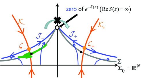
Figure 1: Ergodicity problem. Configurations can hardly move from a vicinity of one thimble ${\mathcal{J}}_{-}$ to that of another thimble ${\mathcal{J}}_{+}$.

The generalized thimble method [16] is an algorithm which makes a sampling on a deformed surface at such a flow time that is large enough to relax the oscillatory behavior and at the same time is small enough to avoid the ergodicity problem. However, a closer investigation [19] shows that the oscillatory behaviors usually starts being relaxed only after the deformed surface reaches some of the zeros of $e^{-S(z)}$, so that one can hardly expect such an ideal flow time to be found. Nevertheless, this algorithm is still useful for grasping a flow time at which the sign problem starts being relaxed, by observing the average phase factors $\langle e^{-i{\rm Im}\,S(z)}\,dz/|dz|\rangle_{\Sigma_{t}}$ at various flow times. Configurations on (a connected component of) a deformed surface $\Sigma_{t}$ can be generated efficiently with the Hybrid Monte Carlo algorithm [20, 21], which we refer in this paper to the Generalized-thimble Hybrid Monte Carlo (GT-HMC).

The tempered Lefschetz thimble (TLT) method [17] avoids the above dilemma by implementing the tempering algorithm with the flow time as the tempering parameter. This is the first algorithm that solves the sign and ergodicity problems simultaneously, but has a drawback of large computational cost [$O(N^{3})$ for generating a configuration]. The Worldvolume Hybrid Monte Carlo (WV-HMC) method [22] was then introduced to reduce the computational cost of the TLT method while still retaining its advantages. This is based on the molecular dynamics on a continuous accumulation (worldvolume) of deformed surfaces (see Fig. 2). The TLT and WV-HMC methods have been successfully applied to $(0+1)$-dimensional Thirring model [17], the Hubbard model away from half filling [19] and the Stephanov model [22] (although the system sizes are yet small).

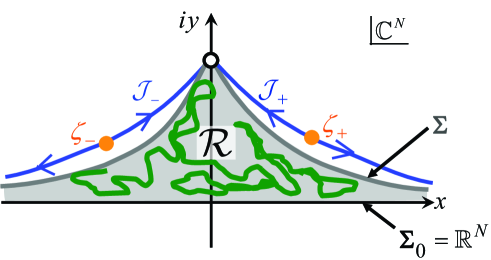
Figure 2: Worldvolume $\mathcal{R}$.

3 Generalized-thimble Hybrid Monte Carlo (GT-HMC)

We explain the basics of GT-HMC [20, 21] and propose its simplified algorithm. In the following, $\Sigma\equiv\Sigma_{t}$ is the deformed surface at flow time $t$, and $T_{z}\Sigma$ and $N_{z}\Sigma$ represent the tangent and normal spaces at $z$ to $\Sigma$, respectively.

3.1 Path-integral form for GT-HMC

We start from the expression [eq. (2.5)]

$$\langle{\mathcal{O}}\rangle =\frac{\int_{\Sigma}dz\,e^{-S(z)}\,{\mathcal{O}}(z)}{\int_{\Sigma}dz\,e^{-S(z)}}.$$ (3.1)

With local coordinates $x=(x^{a})$ $(a=1,\ldots,N)$ and the Jacobian $E^{i}_{a}\equiv\partial z^{i}/\partial x^{a}$, the holomorphic $N$-form $dz=dz^{1}\wedge\cdots\wedge dz^{N}$ is expressed as

$$dz=\det E\,dx.$$ (3.2)

We introduce the inner product

$$\langle u,v\rangle\equiv{\rm Re\,}u^{\dagger}v=\sum_{i=1}^{N}{\rm Re\,}\overline{u^{i}}v^{i}\,\,\bigl{(}=\langle v,u\rangle\bigr{)}$$ (3.3)

for vectors $u=(u^{i}),\,v=(v^{i})\in{\mathbb{C}}^{N}$. The induced metric $ds^{2}=\gamma_{ab}\,dx^{a}dx^{b}\equiv|dz(x)|^{2}$ is then given by

$$\gamma_{ab}=\langle E_{a},E_{b}\rangle=E_{a}^{\dagger}E_{b},$$ (3.4)

which yields the invariant volume element on $\Sigma$,

$$|dz|\equiv\sqrt{\gamma}\,dx=|\det E\,|\,dx.$$ (3.5)

The expectation value (3.1) is then expressed as a ratio of reweighted averages on $\Sigma$:

$$\langle{\mathcal{O}}\rangle=\frac{\langle{\mathcal{F}}(z)\,{\mathcal{O}}(z)\rangle_{\Sigma}}{\langle{\mathcal{F}}(z)\rangle_{\Sigma}},$$ (3.6)

where $\langle\cdots\rangle_{\Sigma}$ is defined by

$$\langle g(z)\rangle_{\Sigma}\equiv\frac{\int_{\Sigma}|dz|\,e^{-{\rm Re}\,S(z)}\,g(z)}{\int_{\Sigma}|dz|\,e^{-{\rm Re}\,S(z)}}$$ (3.7)

and ${\mathcal{F}}(z)$ is the associated reweighting factor:

$${\mathcal{F}}(z)\equiv\frac{dz}{|dz|}\,e^{-i\,{\rm Im}\,S(z)}=\frac{\det E}{|\det E\,|}\,e^{-i\,{\rm Im}\,S(z)}.$$ (3.8)

The reweighted average $\langle\cdots\rangle_{\Sigma}$ can be written as a path integral over the phase space by rewriting the measure $|dz|=\sqrt{\gamma}\,dx$ to the form

$$|dz|=\sqrt{\gamma}\,dx\propto dx\,dp\,e^{-(1/2)\,\gamma^{ab}\,p_{a}p_{b}},$$ (3.9)

where $dx\,dp\equiv\prod_{a}\bigl{(}dx^{a}dp_{a}\bigr{)}$ is the volume element of the phase space. We thus obtain the phase-space path integral in the parameter-space representation:

$$\langle g(z)\rangle_{\Sigma}=\frac{\int dx\,dp\,e^{-(1/2)\,\gamma^{ab}\,p_{a}p_{b}-{\rm Re}\,S(z(x))}\,g(z(x))}{\int dx\,dp\,e^{-(1/2)\,\gamma^{ab}\,p_{a}p_{b}-{\rm Re}\,S(z(x))}}.$$ (3.10)

Note that the volume element can be expressed as $dx\,dp=\omega^{N}/N!$ with the symplectic 2-form $\omega\equiv dp_{a}\wedge dx^{a}$.

In Monte Carlo calculations, it is more convenient to rewrite everything in terms of the target space coordinates $z=(z^{i})$. To do this, we introduce the momentum $\pi=(\pi^{i})$ which is tangent to $\Sigma$:

$$\pi^{i}\equiv p^{a}E_{a}^{i}\in T_{z}\Sigma\quad(p^{a}\equiv\gamma^{ab}\,p_{b}).$$ (3.11)

One then can show that the 1-form

$$a\equiv\langle\pi,dz\rangle={\rm Re}\,\overline{\pi^{i}}\,dz^{i}$$ (3.12)

can be expressed as $a=p_{a}dx^{a}$, and thus we find that $a$ is a symplectic potential of $\omega$:

$$\omega=da={\rm Re}\,d\overline{\pi^{i}}\wedge dz^{i}.$$ (3.13)

Furthermore, noting the identity

$$\langle\pi,\pi\rangle=\gamma^{ab}p_{a}p_{b}\quad(\pi\in T_{z}\Sigma),$$ (3.14)

we have the following target-space representation:

$$\langle g(z)\rangle=\frac{\int_{T\Sigma}\,\omega^{N}\,e^{-H(z,\pi)}\,g(z)}{\int_{T\Sigma}\,\omega^{N}\,e^{-H(z,\pi)}}.$$ (3.15)

Here, $T\Sigma\equiv\{(z,\pi)\,|\,z\in\Sigma,\,\pi\in T_{z}\Sigma\}$ is the tangent bundle of $\Sigma$, and $H(z,\pi)$ is the Hamiltonian of the form

$$H(z,\pi)=\frac{1}{2}\,\langle\pi,\pi\rangle+V(z)$$ (3.16)

with the (real-valued) potential

$$V(z)={\rm Re}\,S(z)=\frac{1}{2}\,[S(z)+\overline{S(z)}].$$ (3.17)

3.2 Constrained molecular dynamics on $\Sigma$

We assume that the $N$-dimensional real submanifold $\Sigma$ in ${\mathbb{C}}^{N}={\mathbb{R}}^{2N}$ is specified by $N$ independent equations $\phi^{r}(z)=0$ $(r=1,\ldots,N)$ with real-valued functions $\phi^{r}(z)$. In order to define a consistent molecular dynamics on $\Sigma$, we consider the Hamilton dynamics for an action of the first-order form:

$$I[z,\pi,\lambda]=\int ds\,\Bigl{[}\langle\pi,{\overset{\circ}{z}}\rangle-H(z,\pi)-\lambda_{r}\,\phi^{r}(z)\Bigr{]}.$$ (3.18)

Here, ${\overset{\circ}{z}}\equiv dz/ds$, and $\lambda_{r}\in{\mathbb{R}}$ are Lagrange multipliers. Hamilton’s equations are then given by

$${\overset{\circ}{z}} =\pi,$$ (3.19)

$${\overset{\circ}{\pi}} =-2\overline{\partial V(z)}-2\lambda_{r}\,\overline{\partial\phi^{r}(z)}$$ (3.20)

with constraints

$$\phi^{r}(z) =0,$$ (3.21)

$$\langle\pi,\overline{\partial\phi^{r}}\rangle =0.$$ (3.22)

One can easily show that the symplectic potential $a$ changes under molecular dynamics as ${\overset{\circ}{a}}=d[(1/2)\langle\pi,\pi\rangle-V(z)]$, from which follows ${\overset{\circ}{\omega}}=d{\overset{\circ}{a}}=0$. Furthermore, noting that $\lambda\equiv\lambda_{r}\,\overline{\partial\phi^{r}(z)}\in N_{z}\Sigma$, one can also show that ${\overset{\circ}{H}}=0$.

A discretized form of (3.19)–(3.20) with step size $\Delta s$ is given by RATTLE [36, 37] of the following form (we rescale $\lambda\to\lambda/\Delta s$ for later convenience) [12, 20, 21]:

$$\pi_{1/2} =\pi-\Delta s\,\overline{\partial V(z)}-\lambda/\Delta s,$$ (3.23)

$$z^{\prime} =z+\Delta s\,\pi_{1/2},$$ (3.24)

$$\pi^{\prime} =\pi_{1/2}-\Delta s\,\overline{\partial V(z^{\prime})}-\lambda^{\prime}/\Delta s.$$ (3.25)

Here, the Lagrange multipliers $\lambda\in N_{z}\Sigma$ and $\lambda^{\prime}\in N_{z^{\prime}}\Sigma$ are determined such that $z^{\prime}\in\Sigma$ and $\pi^{\prime}\in T_{z^{\prime}}\Sigma$, respectively. One easily sees that the transformation $(z,\pi)\to(z^{\prime},\pi^{\prime})$ satisfies the reversibility. Noting that $\langle\lambda,dz\rangle=0$ and $\langle\lambda^{\prime},dz^{\prime}\rangle=0$, one can also show that the symplectic potential $a=\langle\pi,dz\rangle$ transforms as follows:

$$a_{1/2} \equiv\langle\pi_{1/2},dz\rangle=a-(\Delta s/2)\,dV(z),$$ (3.26)

$$a^{\prime}_{1/2} \equiv\langle\pi_{1/2},dz^{\prime}\rangle=a_{1/2}+(\Delta s/2)\,d\langle\pi_{1/2},\pi_{1/2}\rangle,$$ (3.27)

$$a^{\prime} \equiv\langle\pi^{\prime},dz^{\prime}\rangle=a^{\prime}_{1/2}-(\Delta s/2)\,dV(z^{\prime})$$

$$=a+(\Delta s/2)\,d\bigl{[}\langle\pi_{1/2},\pi_{1/2}\rangle-V(z)-V(z^{\prime})\bigr{]},$$ (3.28)

from which we find that this transformation is symplectic ($\omega^{\prime}=\omega$) and thus volume-preserving ($\omega^{\prime N}=\omega^{N}$). One can further show that this transformation preserves the Hamiltonian to $O(\Delta s^{2})$:

$$H(z^{\prime},\pi^{\prime})=H(z,\pi)+O(\Delta s^{3}).$$ (3.29)

3.3 Projector in GT-HMC

As we see in the next subsection, in determining $\lambda$ and $\lambda^{\prime}$, we repeatedly project a vector $w\in T_{z}{\mathbb{C}}^{N}$ onto the tangent space $T_{z}\Sigma$ and the normal space $N_{z}\Sigma$:

$$w=v+n\quad\bigl{[}v\in T_{z}\Sigma,~{}n\in N_{z}\Sigma\bigr{]}.$$ (3.30)

This projection can be carried out by an iterative use of flow as follows [12]. For $z\in\Sigma$ and its starting configuration $x\in\Sigma_{0}={\mathbb{R}}^{N}$, we introduce an ${\mathbb{R}}$-linear map $A:\,T_{x}{\mathbb{C}}^{N}\to T_{z}{\mathbb{C}}^{N}$ which consists of three steps (see Fig. 3):

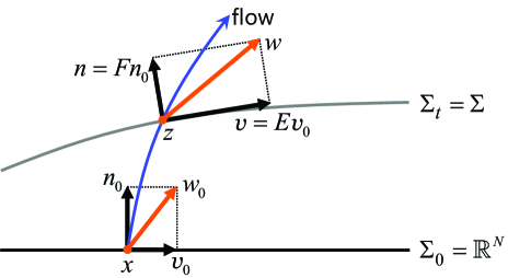
Figure 3: Linear transformation: $w_{0}=v_{0}+n_{0}\mapsto w=Ev_{0}+Fn_{0}$.

(1)  For a given vector $w_{0}\in T_{x}{\mathbb{C}}^{N}$, decompose it into

$$v_{0}\equiv\frac{1}{2}\,(w_{0}+\bar{w}_{0})\in T_{x}\Sigma_{0},\quad n_{0}\equiv\frac{1}{2}\,(w_{0}-\bar{w}_{0})\in N_{x}\Sigma_{0}.$$ (3.31)

(2)  Integrate the following flow equations that maps $v_{0}\in T_{x}\Sigma_{0}$ to $v\in T_{z}\Sigma$ and $n_{0}\in N_{x}\Sigma_{0}$ to $n\in N_{z}\Sigma$,

$$\dot{z} =\overline{\partial S(z)}\mbox{~{}~{}with~{}~{}}z|_{t=0}=x,$$ (3.32)

$$\dot{v} =\overline{H(z)\,v}\mbox{~{}~{}with~{}~{}}v|_{t=0}=v_{0},$$ (3.33)

$$\dot{n} =-\overline{H(z)\,n}\mbox{~{}~{}with~{}~{}}n|_{t=0}=n_{0},$$ (3.34)

where $H(z)\equiv(\partial_{i}\partial_{j}S(z))$ is the Hessian matrix. Note that $v$ and $n$ are linear in $v_{0}$ and $n_{0}$, respectively, and we write them as

$$v^{i}\equiv E^{i}_{a}v_{0}^{a}=(Ev_{0})^{i},\quad n^{i}\equiv F^{i}_{a}n_{0}^{a}=(Fn_{0})^{i}.$$ (3.35)

(3)  Define an ${\mathbb{R}}$-linear map $A:\,T_{x}{\mathbb{C}}^{N}\ni w_{0}\mapsto w\in T_{z}{\mathbb{C}}^{N}$ by

$$w=Aw_{0}\equiv Ev_{0}+Fn_{0}\mbox{~{}~{}for~{}~{}$w_{0}=v_{0}+n_{0}$}.$$ (3.36)

Once the map $A$ is defined, the decomposition (3.30) can be carried out for a given $w\in T_{z}{\mathbb{C}}^{N}$ as follows:

Step 1.  Solve the linear problem $Aw_{0}=w$ with respect to $w_{0}$.

Step 2.  Decompose $w_{0}$ into $v_{0}=(1/2)(w_{0}+\bar{w}_{0})$ and $n_{0}=(1/2)(w_{0}-\bar{w}_{0})$.

Step 3.  Compute $v=Ev_{0}$ and $n=Fn_{0}$ by integrating the flow equations (3.32)–(3.34).

Note that, if we use an iterative method (such as BiCGStab) for solving $Aw_{0}=w$ in Step 1, we no longer need to carry out Step 2 and Step 3. This is because in Step 1 we repeatedly compute $E\tilde{v}_{0}$ and $F\tilde{n}_{0}$ for a candidate solution $\tilde{w}_{0}=\tilde{v}_{0}+\tilde{n}_{0}$, so that $v=Ev_{0}$ and $n=Fn_{0}$ are already obtained when the iteration is converged.

3.4 RATTLE in GT-HMC

The Lagrange multiplies $\lambda\in N_{z}\Sigma$ and $\lambda^{\prime}\in N_{z^{\prime}}\Sigma$ in (3.23)–(3.25) are determined as follows. This subsection is one of the main parts of this paper.

3.4.1 Determination of $\lambda$

The condition that $z^{\prime}\in\Sigma$ is equivalent to that $z^{\prime}$ can be written as $z^{\prime}=z_{t}(x^{\prime})$ with $x^{\prime}\in\Sigma_{0}$ (see Fig. 4).

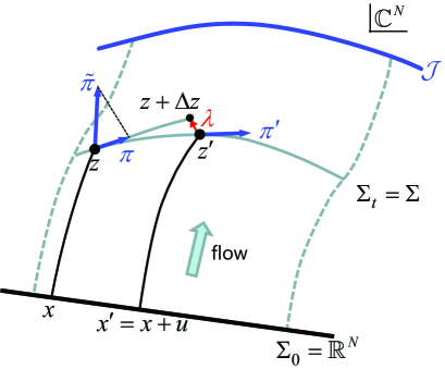
Figure 4: RATTLE in GT-HMC.

Thus, finding $\lambda$ satisfying (3.23) and (3.24) for a given $z=z_{t}(x)\in\Sigma$ and $\pi\in T_{z}\Sigma$ is equivalent to finding a doublet $(u,\lambda)$ $(u\in T_{x}\Sigma_{0},\,\lambda\in N_{z}\Sigma)$ that satisfies

$$z_{t}(x+u)=z_{t}(x)+\Delta z-\lambda$$ (3.37)

with

$$\Delta z(z,\pi)\equiv\Delta s\,\pi-(\Delta s)^{2}\,\overline{\partial V(z)}.$$ (3.38)

Equation (3.37) can be solved iteratively with Newton’s method. There, one solves the following linearized equation in updating an approximate solution $(u,\lambda)$ as $u\leftarrow u+\Delta u$ and $\lambda\leftarrow\lambda+\Delta\lambda$:

$$E_{\rm new}\Delta u+\Delta\lambda=B,$$ (3.39)

where $E_{\rm new}\equiv\partial z_{t}(x+u)/\partial u=(\partial z_{t}/\partial x)(x+u)$, and

$$B\equiv z+\Delta z-\lambda-z_{\rm new}\in{\mathbb{C}}^{N}$$ (3.40)

with $z_{\rm new}\equiv z_{t}(x+u)$.

Equation (3.39) is proposed in [21], and can be solved with direct or iterative methods by regarding it as a linear equation of the form $AX=B$ with respect to $X=(\Delta u,\Delta\lambda)$. Instead of solving (3.39), we here propose to use the simplified Newton equation, where $E_{\rm new}$ on the left hand side is replaced by the value at $z=z_{t}(x)$:

$$E\Delta u+\Delta\lambda=B.$$ (3.41)

This equation can be readily solved by using the projection introduced in Sect. 3.3. To see this, from the decomposition

$$B= B_{v}+B_{n}=EB_{0,v}+FB_{0,n}$$ (3.42)

with $B_{v}\in T_{z}\Sigma$, $B_{n}\in N_{z}\Sigma$, $B_{0,v}\in T_{x}\Sigma_{0}$ and $B_{0,n}\in N_{x}\Sigma_{0}$, we write $B$ to the form

$$B=EB_{0,v}+B_{n}.$$ (3.43)

Then, comparing with the left hand side of (3.41), we obtain

$$\Delta u=B_{0,v},\quad\Delta\lambda=B_{n}.$$ (3.44)

Furthermore, since $u$, $\lambda$, $\Delta z$ are at least of $O(\Delta s)$, the solution $(\tilde{u},\tilde{\lambda})$ to the equation

$$E\tilde{u}+\tilde{\lambda}=\Delta z$$ (3.45)

should solve (3.37) approximately and can be used as an initial guess of the iteration. Noting that (3.45) takes the same form as (3.41) with $B$ replaced by $\Delta z$, we find that $(\tilde{u},\tilde{\lambda})$ are obtained from the decomposition $\Delta z=E(\Delta z)_{0,v}+(\Delta z)_{n}$ as

$$\tilde{u}=(\Delta z)_{0,v},\quad\tilde{\lambda}=(\Delta z)_{n}.$$ (3.46)

3.4.2 Determination of $\lambda^{\prime}$

Note that determining $\lambda^{\prime}$ in (3.25) such that $\pi^{\prime}\in T_{z^{\prime}}\Sigma$ is equivalent to projecting $\tilde{\pi}^{\prime}\equiv\pi_{1/2}-\Delta s\,\overline{\partial V(z^{\prime})}$ onto $T_{z^{\prime}}\Sigma$. Thus, $\pi^{\prime}$ is simply obtained from the decomposition $\tilde{\pi}^{\prime}=\tilde{\pi}^{\prime}_{v}+\tilde{\pi}^{\prime}_{n}$ as $\pi^{\prime}=\tilde{\pi}^{\prime}_{v}$.

Molecular dynamics from a configuration $(z,\pi)\in T\Sigma$ is summarized in Algorithm 1.

Algorithm 1 Simplified Newton for the RATTLE $(z,\pi)\to(z^{\prime},\pi^{\prime})$ in GT-HMC

1:Compute $\Delta z=\Delta s\,\pi-(\Delta s)^{2}\,\overline{\partial V(z)}$

2:Decompose $\Delta z$ into $\Delta z=E(\Delta z)_{0,v}+(\Delta z)_{n}$

3:Set $u=(\Delta z)_{0,v}$ and $\lambda=(\Delta z)_{n}$

4:for $k=0,1,\ldots$ do

5:     Set $z_{\rm new}=z_{t}(x+u)$ and $B=z+\Delta z-\lambda-z_{\rm new}$

6:     if $|B|$ is small then

7:         break

8:     end if

9:     Decompose $B$ into $B=EB_{0,v}+B_{n}$

10:     Set $\Delta u=B_{0,v}$ and $\Delta\lambda=B_{n}$

11:     $u\leftarrow u+\Delta u$ and $\lambda\leftarrow\lambda+\Delta\lambda$

12:end for

13:Set $z^{\prime}=z_{\rm new}$ and $\tilde{\pi}^{\prime}=\pi-\Delta s\,[\overline{\partial V(z)}+\overline{\partial V(z^{\prime})}]-\lambda/\Delta s$

14:Decompose $\tilde{\pi}^{\prime}\in T_{z^{\prime}}{\mathbb{C}}^{N}$ into $\tilde{\pi}^{\prime}=\tilde{\pi}^{\prime}_{v}+\tilde{\pi}^{\prime}_{n}$ and set $\pi^{\prime}=\tilde{\pi}^{\prime}_{v}$

3.5 Summary of GT-HMC

We summarize in Algorithm 2 the GT-HMC algorithm for updating a configuration $z\in\Sigma$ with the RATTLE of Algorithm 1.

Algorithm 2 GT-HMC

1:Given $z\in\Sigma$, generate $\tilde{\pi}\in T_{z}{\mathbb{C}}^{N}$ from the distribution $\propto e^{-\tilde{\pi}^{\dagger}\tilde{\pi}/2}$

2:Decompose $\tilde{\pi}$ into $\tilde{\pi}=\tilde{\pi}_{v}+\tilde{\pi}_{n}$ and set $\pi=\tilde{\pi}_{v}$

3:Repeat the RATTLE of Algorithm 1 to obtain $(z,\pi)\to(z^{\prime},\pi^{\prime})$

4:Compute $\Delta H\equiv H(z^{\prime},\pi^{\prime})-H(z,\pi)$ and accept $(z^{\prime},\pi^{\prime})$ as a new configuration with probability $\min(1,e^{-\Delta H})$, otherwise use $(z,\pi)$ again as a new configuration

4 Worldvolume Hybrid Monte Carlo (WV-HMC)

We explain the basics of WV-HMC [22] and propose its simplified algorithm. For convenience of the reader who reads only this section, the presentation is made in a completely parallel way to that for GT-HMC without worrying about repetition.

4.1 Path-integral form for WV-HMC

We restart from the expression (2.5):

$$\langle{\mathcal{O}}\rangle=\frac{\int_{\Sigma_{t}}dz_{t}\,e^{-S(z_{t})}\,{\mathcal{O}}(z_{t})}{\int_{\Sigma_{t}}dz_{t}\,e^{-S(z_{t})}},$$ (4.1)

where we have denoted the configurations by $z_{t}$ (instead of $z$) to stress that they live on $\Sigma_{t}$. Since the numerator and the denominator are both independent of $t$ (Cauchy’s theorem), they can be averaged over flow time $t$ with an arbitrary weight $e^{-W(t)}$, leading to the expression [22]

$$\langle{\mathcal{O}}\rangle =\frac{\int dt\,e^{-W(t)}\,\int_{\Sigma_{t}}dz_{t}\,e^{-S(z_{t})}\,{\mathcal{O}}(z_{t})}{\int dt\,e^{-W(t)}\,\int_{\Sigma_{t}}dz_{t}\,e^{-S(z_{t})}}$$

$$\equiv\frac{\int_{{\mathcal{R}}}dt\,dz_{t}\,e^{-S(z_{t})-W(t)}\,{\mathcal{O}}(z_{t})}{\int_{{\mathcal{R}}}dt\,dz_{t}\,e^{-S(z_{t})-W(t)}}\equiv\frac{Z_{{\mathcal{O}}}}{Z}.$$ (4.2)

The $(N+1)$-dimensional integration region ${\mathcal{R}}$ is defined by ${\mathcal{R}}\equiv\{z_{t}\in\Sigma_{t}\,|\,t\in{\mathbb{R}}\}$, which we refer to the worldvolume, by regarding it as an orbit of an integration surface $\Sigma_{t}$ in the target space ${\mathbb{C}}^{N}={\mathbb{R}}^{2N}$. The extension of ${\mathcal{R}}$ in the flow time direction can be effectively constrained to a finite interval $[T_{0},T_{1}]$ by adjusting the functional form of $W(t)$. The function $W(t)$ has another role to lift configurations upwards (positive flow direction) so that they are distributed almost equally over different flow times. In fact, the force of molecular dynamics exerts configurations in the direction opposite to the flow [see, e.g., eq. (3.20) with $-2\overline{\partial V(z)}=-\,\overline{\partial S(z)}$] and thus configurations have a tendency to precipitate towards the bottom (near $\Sigma_{0}$) if nothing is done. A possible form of $W(t)$ is given in Sect. 4.5 (see [33] for a more detailed study).

Since multimodality becomes more severe at larger flow times, we take the lower bound $T_{0}$ to be small enough such that there is no ergodicity problem on $\Sigma_{T_{0}}$. The upper bound $T_{1}$ is chosen such that oscillatory integrals are sufficiently tamed there. After global equilibrium is well established over ${\mathcal{R}}$, we estimate the expectation value $\langle\mathcal{O}\rangle$ by sample averages using the configurations taken from a subinterval $[\tilde{T}_{0},\tilde{T}_{1}]$ ($T_{0}\leq\tilde{T}_{0}<\tilde{T}_{1}\leq T_{1}$), where both the sign and ergodicity problems disappear.

With local coordinates $x=(x^{a})$ for $\Sigma_{t}$ (see footnote 4), we introduce those of ${\mathcal{R}}$ as $\hat{x}=(\hat{x}^{\mu})=(\hat{x}^{0}=t,\hat{x}^{a}=x^{a})$. Then, the induced metric on ${\mathcal{R}}$, $d\hat{s}^{2}=\hat{\gamma}_{\mu\nu}\,d\hat{x}^{\mu}d\hat{x}^{\nu}\equiv|dz(\hat{x})|^{2}$, takes the following form [22]:

$$d\hat{s}^{2} =|\partial_{t}z^{i}\,dt+\partial_{x^{a}}z^{i}\,dx^{a}|^{2}=|\xi^{i}dt+E_{a}^{i}dx^{a}|^{2}=|\xi^{i}_{n}dt+(E_{a}^{i}dx^{a}+\xi_{v}^{i}dt)|^{2}$$

$$=\alpha^{2}\,dt^{2}+\gamma_{ab}\,(dx^{a}+\beta^{a}dt)\,(dx^{b}+\beta^{b}dt)$$ (4.3)

with the induced metric $\gamma_{ab}$ on $\Sigma_{t}$, the shift $\beta^{a}$ and the lapse $\alpha\,(>0)$ given by

$$\gamma_{ab} =\langle E_{a},E_{b}\rangle,$$ (4.4)

$$\beta^{a} =\gamma^{ab}\,\langle\xi,E_{b}\rangle,$$ (4.5)

$$\alpha^{2} =\langle\xi_{n},\xi_{n}\rangle.$$ (4.6)

Here, $E_{a}=(\partial z^{i}/\partial x^{a})$ form a basis of $T_{z}\Sigma_{t}$, and $\xi=\overline{\partial S}$ is the flow vector, which is decomposed into the tangential and normalized components as $\xi=\xi_{v}+\xi_{n}$ [see eq. (3.30)]. Note that $\xi_{v}=E_{a}\,\beta^{a}\in T_{z}\Sigma_{t}\,(\subset T_{z}{\mathcal{R}})$ and $\xi_{n}\in N_{z}\Sigma_{t}\cap T_{z}{\mathcal{R}}$. The invariant volume element on ${\mathcal{R}}$ is then given by

$$|dz|_{\mathcal{R}}\equiv\sqrt{\hat{\gamma}}\,d\hat{x}=\alpha\sqrt{\gamma}\,dt\,dx=\alpha\,|dz_{t}|\,dt,$$ (4.7)

and $Z_{\mathcal{O}}$ in (4.2) can be written as

$$Z_{\mathcal{O}}=\int_{\mathcal{R}}|dz|_{\mathcal{R}}\,e^{-V(z)}\,{\mathcal{F}}(z)\,{\mathcal{O}}(z)$$ (4.8)

with

$$V(z) \equiv{\rm Re}\,S(z)+W(t(z)),$$ (4.9)

$${\mathcal{F}}(z) \equiv\frac{dt\,dz_{t}}{|dz|_{\mathcal{R}}}\,e^{-i\,{\rm Im}\,S(z)}=\alpha^{-1}\,\frac{dz_{t}}{|dz_{t}|}\,e^{-i\,{\rm Im}\,S(z)}.$$ (4.10)

Thus, by defining the reweighted average $\langle\cdots\rangle_{\mathcal{R}}$ on ${\mathcal{R}}$ by

$$\langle g(z)\rangle_{\mathcal{R}}\equiv\frac{\int_{\mathcal{R}}|dz|_{\mathcal{R}}\,e^{-V(z)}\,g(z)}{\int_{\mathcal{R}}|dz|_{\mathcal{R}}\,e^{-V(z)}},$$ (4.11)

the expectation value (4.2) is expressed as a ratio of the reweighted averages:

$$\langle{\mathcal{O}}\rangle=\frac{\langle{\mathcal{F}}(z)\,{\mathcal{O}}(z)\rangle_{\mathcal{R}}}{\langle{\mathcal{F}}(z)\rangle_{\mathcal{R}}}.$$ (4.12)

Similarly to the GT-HMC algorithm, the reweighted averages $\langle\cdots\rangle_{\mathcal{R}}$ can be written as a path integral over the phase space by rewriting the measure $|dz|_{\mathcal{R}}=\sqrt{\hat{\gamma}}\,d\hat{x}$ to the form

$$|dz|_{\mathcal{R}}=\sqrt{\hat{\gamma}}\,d\hat{x}\propto d\hat{x}\,d\hat{p}\,e^{-(1/2)\,\hat{\gamma}^{\mu\nu}\,\hat{p}_{\mu}\hat{p}_{\nu}},$$ (4.13)

where $d\hat{x}\,d\hat{p}\equiv\prod_{\mu}\bigl{(}d\hat{x}^{\mu}d\hat{p}_{\mu}\bigr{)}$ is the volume element of the phase space of ${\mathcal{R}}$. We thus obtain the phase-space path integral in the parameter-space representation:

$$\langle g(z)\rangle_{\mathcal{R}}=\frac{\int d\hat{x}\,d\hat{p}\,e^{-(1/2)\,\hat{\gamma}^{\mu\nu}\,\hat{p}_{\mu}\hat{p}_{\nu}-V(z(\hat{x}))}\,g(z(\hat{x}))}{\int d\hat{x}\,d\hat{p}\,e^{-(1/2)\,\hat{\gamma}^{\mu\nu}\,\hat{p}_{\mu}\hat{p}_{\nu}-V(z(\hat{x}))}}.$$ (4.14)

Note that the volume element can be expressed as $d\hat{x}\,d\hat{p}=\hat{\omega}^{N+1}/(N+1)!$ with the symplectic 2-form $\hat{\omega}\equiv d\hat{p}_{\mu}\wedge d\hat{x}^{\mu}$.

In Monte Carlo calculations, it is more convenient to rewrite everything in terms of the target space coordinates $z=(z^{i})$. To do this, we introduce the momentum $\pi=(\pi^{i})$ which is tangent to ${\mathcal{R}}$:

$$\pi^{i}\equiv\hat{p}^{\mu}\hat{E}_{\mu}^{i}\in T_{z}{\mathcal{R}}\quad(\hat{p}^{\mu}\equiv\hat{\gamma}^{\mu\nu}\,\hat{p}_{\nu}).$$ (4.15)

One then can show that the 1-form

$$\hat{a}\equiv\langle\pi,dz\rangle={\rm Re}\,\overline{\pi^{i}}\,dz^{i}$$ (4.16)

can be expressed as $\hat{a}=\hat{p}_{\mu}d\hat{x}^{\mu}$, and thus we find that $\hat{a}$ is a symplectic potential of $\hat{\omega}$:

$$\hat{\omega}=d\hat{a}={\rm Re}\,d\overline{\pi^{i}}\wedge dz^{i}.$$ (4.17)

Furthermore, noting the identity

$$\langle\pi,\pi\rangle=\hat{\gamma}^{\mu\nu}\hat{p}_{\mu}\hat{p}_{\nu}\quad(\pi\in T_{z}{\mathcal{R}}),$$ (4.18)

we have the following target-space representation:

$$\langle g(z)\rangle_{\mathcal{R}}=\frac{\int_{T{\mathcal{R}}}\,\hat{\omega}^{N+1}\,e^{-H(z,\pi)}\,g(z)}{\int_{T{\mathcal{R}}}\,\hat{\omega}^{N+1}\,e^{-H(z,\pi)}}.$$ (4.19)

Here, $T{\mathcal{R}}\equiv\{(z,\pi)\,|\,z\in{\mathcal{R}},\,\pi\in T_{z}{\mathcal{R}}\}$ is the tangent bundle of ${\mathcal{R}}$, and $H(z,\pi)$ is the Hamiltonian of the form

$$H(z,\pi)=\frac{1}{2}\,\langle\pi,\pi\rangle+V(z)$$ (4.20)

with the (real-valued) potential

$$V(z)={\rm Re}\,S(z)+W(t(z)).$$ (4.21)

4.2 Constrained molecular dynamics on ${\mathcal{R}}$

In parallel to discussions for GT-HMC, the RATTLE [36, 37] for WV-HMC is given as follows [22]:

$$\pi_{1/2} =\pi-\Delta s\,\overline{\partial V(z)}-\lambda/\Delta s,$$ (4.22)

$$z^{\prime} =z+\Delta s\,\pi_{1/2},$$ (4.23)

$$\pi^{\prime} =\pi_{1/2}-\Delta s\,\overline{\partial V(z^{\prime})}-\lambda^{\prime}/\Delta s.$$ (4.24)

Here, the Lagrange multipliers $\lambda\in N_{z}{\mathcal{R}}$ and $\lambda^{\prime}\in N_{z^{\prime}}{\mathcal{R}}$ are determined such that $z^{\prime}\in{\mathcal{R}}$ and $\pi^{\prime}\in T_{z^{\prime}}{\mathcal{R}}$, respectively. This transformation satisfies the reversibility as in footnote 9. One can also show that this transformation is symplectic ($\hat{\omega}^{\prime}=\hat{\omega}$) and thus volume-preserving ($\hat{\omega}^{\prime N+1}=\hat{\omega}^{N+1}$). One can further show that it preserves the Hamiltonian to $O(\Delta s^{2})$: $H(z^{\prime},\pi^{\prime})=H(z,\pi)+O(\Delta s^{3})$.

The gradient of the potential, $\overline{\partial V(z)}$, can be set to the form [22]

$$\overline{\partial V(z)}=\frac{1}{2}\,\Bigl{[}\xi+\frac{W^{\prime}(t)}{\langle\xi_{n},\xi_{n}\rangle}\,\xi_{n}\Bigr{]}.$$ (4.25)

A simplified proof is given in Appendix A.

4.3 Projector in WV-HMC

As we see in the next subsection, in determining $\lambda$ and $\lambda^{\prime}$, we repeatedly project a vector $w\in T_{z}{\mathbb{C}}^{N}$ onto the tangent space $T_{z}{\mathcal{R}}$ and the normal space $N_{z}{\mathcal{R}}$:

$$w=w_{\parallel}+w_{\perp}\quad\bigl{[}w_{\parallel}\in T_{z}{\mathcal{R}},~{}w_{\perp}\in N_{z}{\mathcal{R}}\bigr{]}.$$ (4.26)

This decomposition can be carried out by using the projection for $\Sigma=\Sigma_{t}$ [see eq. (3.30)]. To see this, let us decompose the vectors $w$ and $\xi$ into

$$w =w_{v}+w_{n}\quad\bigl{[}w_{v}\in T_{z}\Sigma_{t},~{}w_{n}\in N_{z}\Sigma_{t}\bigr{]},$$ (4.27)

$$\xi =\xi_{v}+\xi_{n}\quad\bigl{[}\xi_{v}\in T_{z}\Sigma_{t},~{}\xi_{n}\in N_{z}\Sigma_{t}\bigr{]},$$ (4.28)

and set

$$c=\frac{\langle\xi_{n},w_{n}\rangle}{\langle\xi_{n},\xi_{n}\rangle}.$$ (4.29)

Then, $w_{\parallel}$ and $w_{\perp}$ are given by

$$w_{\parallel}=w_{v}+c\,\xi_{n},\quad w_{\perp}=w_{n}-c\,\xi_{n}.$$ (4.30)

4.4 RATTLE in WV-HMC

The Lagrange multiplies $\lambda\in N_{z}{\mathcal{R}}$ and $\lambda^{\prime}\in N_{z^{\prime}}{\mathcal{R}}$ in (4.22)–(4.24) are determined as follows. This subsection is a main part of this paper.

4.4.1 Determination of $\lambda$

The condition that $z^{\prime}\in{\mathcal{R}}$ is equivalent to that $z^{\prime}$ can be written as $z^{\prime}=z_{t^{\prime}}(x^{\prime})$ with some $t^{\prime}\in{\mathbb{R}}$ and $x^{\prime}\in\Sigma_{0}$ (see Fig. 5).

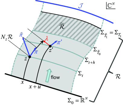
Figure 5: RATTLE in WV-HMC.

Thus, finding $\lambda$ satisfying (4.22) and (4.23) for a given $z=z_{t}(x)\in{\mathcal{R}}$ and $\pi\in T_{z}{\mathcal{R}}$ is equivalent to finding a triplet $(h,u,\lambda)$ $(h\in{\mathbb{R}},\,u\in T_{x}\Sigma_{0},\,\lambda\in N_{z}{\mathcal{R}})$ that satisfies

$$z_{t+h}(x+u)=z_{t}(x)+\Delta z-\lambda$$ (4.31)

with

$$\Delta z(z,\pi)\equiv\Delta s\,\pi-(\Delta s)^{2}\,\overline{\partial V(z)}.$$ (4.32)

Equation (4.31) can be solved iteratively with Newton’s method. There, one solves the following linearized equation in updating an approximate solution $(h,u,\lambda)$ as $h\leftarrow h+\Delta h$, $u\leftarrow u+\Delta u$ and $\lambda\leftarrow\lambda+\Delta\lambda$:

$$\xi_{\rm new}\Delta h+E_{\rm new}\Delta u+\Delta\lambda=B,$$ (4.33)

where $\xi_{\rm new}\equiv\partial z_{t+h}(x+u)/\partial h=(\partial z_{t+h}/\partial t)(x+u)$, $E_{\rm new}\equiv\partial z_{t+h}(x+u)/\partial u=(\partial z_{t+h}/\partial x)(x+u)$, and

$$B\equiv z+\Delta z-\lambda-z_{\rm new}\in{\mathbb{C}}^{N}$$ (4.34)

with $z_{\rm new}\equiv z_{t+h}(x+u)$.

Equation (4.33) is proposed in [22], and can be solved with direct or iterative methods by regarding it as a linear equation of the form $AX=B$ with respect to $X=(\Delta h,\Delta u,\Delta\lambda)$. Instead of solving (4.33), we here propose to use the simplified Newton equation, where $\xi_{\rm new}$ and $E_{\rm new}$ on the left hand side are replaced by the values at $z=z_{t}(x)$:

$$\xi\Delta h+E\Delta u+\Delta\lambda=B.$$ (4.35)

This equation can be readily solved by using the projection introduced in Sect. 4.3. To see this, we introduce the decomposition of $\xi$ and $B$ as

$$\xi =\xi_{\parallel}$$

$$=E\xi_{0,v}+\xi_{n},$$ (4.36)

$$B =B_{\parallel}+B_{\perp}=(B_{v}+c_{B}\,\xi_{n})+(B_{n}-c_{B}\,\xi_{n})$$

$$=EB_{0,v}+c_{B}\,\xi_{n}+(B_{n}-c_{B}\,\xi_{n})$$ (4.37)

with

$$c_{B}\equiv\frac{\langle B,\xi_{n}\rangle}{\langle\xi_{n},\xi_{n}\rangle}.$$ (4.38)

On the other hand, the left hand side of (4.35) is decomposed as

$$\xi\Delta h+E\Delta u+\Delta\lambda =(E\xi_{0,v}+\xi_{n})\,\Delta h+E\Delta u+\Delta\lambda$$

$$=E(\xi_{0,v}\,\Delta h+\Delta u)+\xi_{n}\,\Delta h+\Delta\lambda.$$ (4.39)

Comparing (4.4.1) and (4.39), we find

$$\xi_{0,v}\,\Delta h+\Delta u =B_{0,v},$$ (4.40)

$$\Delta h =c_{B},$$ (4.41)

$$\Delta\lambda =B_{n}-c_{B}\,\xi_{n},$$ (4.42)

or equivalently,

$$\Delta h=c_{B},\quad\Delta u=B_{0,v}-c_{B}\,\xi_{0,v},\quad\Delta\lambda=B_{n}-c_{B}\,\xi_{n}.$$ (4.43)

As in Sect. 3.4.1, an initial guess $(\tilde{h},\,\tilde{u},\tilde{\lambda})$ is obtained by solving the equation

$$\xi\tilde{h}+E\tilde{u}+\tilde{\lambda}=\Delta z.$$ (4.44)

Noting that (4.44) takes the same form as (4.35) with $B$ replaced by $\Delta z$, we obtain $(\tilde{h},\,\tilde{u},\,\tilde{\lambda})$ from the decomposition

$$\Delta z=E(\Delta z)_{0,v}+c_{\Delta z}\,\xi_{n}+[(\Delta z)_{n}-c_{\Delta z}\,\xi_{n}]$$ (4.45)

with

$$c_{\Delta z}\equiv\frac{\langle\Delta z,\xi_{n}\rangle}{\langle\xi_{n},\xi_{n}\rangle}$$ (4.46)

as

$$\tilde{h}=c_{\Delta z},\quad\tilde{u}=(\Delta z)_{0,v}-c_{\Delta z}\,\xi_{0,v},\quad\tilde{\lambda}=(\Delta z)_{n}-c_{\Delta z}\,\xi_{n}.$$ (4.47)

4.4.2 Determination of $\lambda^{\prime}$

Note that determining $\lambda^{\prime}$ in (4.24) such that $\pi^{\prime}\in T_{z^{\prime}}{\mathcal{R}}$ is equivalent to projecting $\tilde{\pi}^{\prime}\equiv\pi_{1/2}-\Delta s\,\overline{\partial V(z^{\prime})}$ onto $T_{z^{\prime}}{\mathcal{R}}$. Thus, $\pi^{\prime}$ is simply obtained from the decomposition $\tilde{\pi}^{\prime}=\tilde{\pi}^{\prime}_{\parallel}+\tilde{\pi}^{\prime}_{\perp}$ as $\pi^{\prime}=\tilde{\pi}^{\prime}_{\parallel}$.

Molecular dynamics from a configuration $(z,\pi)\in T{\mathcal{R}}$ is summarized in Algorithm 3.

Algorithm 3 Simplified Newton for the RATTLE $(z,\pi)\to(z^{\prime},\pi^{\prime})$ in WV-HMC

1:Compute $\xi=\overline{\partial S(z)}$ and $\Delta z=\Delta s\,\pi-(\Delta s)^{2}\,\overline{\partial V(z)}$

2:Decompose $\xi$ and $\Delta z$ into $\xi=E\xi_{0,v}+\xi_{n}$ and $\Delta z=E(\Delta z)_{0,v}+c_{\Delta z}\,\xi_{n}$ with $c_{\Delta z}=\langle\Delta z,\xi_{n}\rangle/\langle\xi_{n},\xi_{n}\rangle$

3:Set $h=c_{\Delta z}$, $u=(\Delta z)_{0,v}-c_{\Delta z}\,\xi_{0,v}$ and $\lambda=(\Delta z)_{n}-c_{\Delta z}\,\xi_{n}$

4:for $k=0,1,\ldots$ do

5:     Set $z_{\rm new}=z_{t+h}(x+u)$ and $B=z+\Delta z-\lambda-z_{\rm new}$

6:     if $|B|$ is small then

7:         break

8:     end if

9:     Decompose $B$ into $B=EB_{0,v}+c_{B}\,\xi_{n}+(B_{n}-c_{B}\,\xi_{n})$ with $c_{B}=\langle B,\xi_{n}\rangle/\langle\xi_{n},\xi_{n}\rangle$

10:     Set $\Delta h=c_{B}$, $\Delta u=B_{0,v}-c_{B}\,\xi_{0,v}$ and $\Delta\lambda=B_{n}-c_{B}\,\xi_{n}$

11:     $h\leftarrow h+\Delta h$, $u\leftarrow u+\Delta u$ and $\lambda\leftarrow\lambda+\Delta\lambda$

12:end for

13:Set $z^{\prime}=z_{\rm new}$ and $\tilde{\pi}^{\prime}=\pi-\Delta s\,[\overline{\partial V(z)}+\overline{\partial V(z^{\prime})}]-\lambda/\Delta s$

14:Decompose $\tilde{\pi}^{\prime}\in T_{z^{\prime}}{\mathbb{C}}^{N}$ into $\tilde{\pi}^{\prime}=\tilde{\pi}^{\prime}_{\parallel}+\tilde{\pi}^{\prime}_{\perp}$ and set $\pi^{\prime}=\tilde{\pi}^{\prime}_{\parallel}$

4.5 Treatment of the boundary

We require configurations in molecular dynamics to be confined in the region $T_{0}\lesssim t\lesssim T_{1}$. This can be realized by adjusting the function $W(t)$, whose possible form, e.g., is (see [33])

$$W(t)=\begin{cases}-\,\gamma(t-T_{0})+c_{0}\,\bigl{(}e^{(t-T_{0})^{2}/2d_{0}^{2}}-1\bigr{)}&(t<T_{0})\\ -\,\gamma(t-T_{0})&(T_{0}\leq t\leq T_{1})\\ -\,\gamma(t-T_{0})+c_{1}\,\bigl{(}e^{(t-T_{1})^{2}/2d_{1}^{2}}-1\bigr{)}&(t>T_{1}).\\ \end{cases}$$ (4.48)

Configurations then bounce off the walls placed at the lower boundary ($t=T_{0})$ and at the upper boundary ($t=T_{1}$) with penetration depths $d_{0}$ and $d_{1}$, respectively ($c_{0}$ and $c_{1}$ correspond to the heights at $t=T_{0}-d_{0}$ and $t=T_{1}+d_{1}$ with the gradients $-\gamma-c_{0}/d_{0}$ and $-\gamma+c_{1}/d_{1}$). However, with a finite step size $\Delta s$, some configurations may penetrate the wall so deeply that the resulting large repulsive force $-W^{\prime}(t)\,\overline{\partial t(z)}$ in $-\overline{\partial V(z)}$ can lower the numerical precision. The simplest solution to this issue, keeping (1) exact volume preservation, (2) exact reversibility, and (3) approximate energy conservation, is to let such a configuration go back the way it just comes [22]. The algorithm will take the form of Algorithm 4.

Algorithm 4 Molecular dynamics step $(z,\pi)\to(z^{\prime},\pi^{\prime})$ in WV-HMC with boundary

1:For a given $(z,\pi)$ with $z=z_{t}(x)$, compute a trial molecular dynamics step $(z,\pi)\to(\tilde{z},\tilde{\pi})$ with $\tilde{z}=z_{\tilde{t}}(\tilde{x})$ using the RATTLE of Algorithm 3

2:if $\tilde{t}<T_{0}-d_{0}$ or $\tilde{t}>T_{1}+d_{1}$ then

3:     Set $z^{\prime}=z$ and $\pi^{\prime}=-\pi$

4:else

5:     Set $z^{\prime}=\tilde{z}$ and $\pi^{\prime}=\tilde{\pi}$

6:end if

4.6 Summary of WV-HMC

We summarize in Algorithm 5 the WV-HMC algorithm for updating a configuration $z\in{\mathcal{R}}$ with the RATTLE of Algorithm 3.

Algorithm 5 WV-HMC

1:Given $z\in{\mathcal{R}}$, generate $\tilde{\pi}\in T_{z}{\mathbb{C}}^{N}$ from the distribution $\propto e^{-\tilde{\pi}^{\dagger}\tilde{\pi}/2}$

2:Decompose $\tilde{\pi}$ into $\tilde{\pi}=\tilde{\pi}_{\parallel}+\tilde{\pi}_{\perp}$ and set $\pi=\tilde{\pi}_{\parallel}$

3:Repeat the RATTLE of Algorithms 3 and 4 to obtain $(z,\pi)\to(z^{\prime},\pi^{\prime})$

4:Compute $\Delta H\equiv H(z^{\prime},\pi^{\prime})-H(z,\pi)$ and accept $(z^{\prime},\pi^{\prime})$ as a new configuration with probability $\min(1,e^{-\Delta H})$, otherwise use $(z,\pi)$ again as a new configuration

5 Numerical test of convergence

In this section, we perform a numerical test for the convergence of the simplified Newton method, and show that the convergence depends on the system size only weakly. We give a discussion only for the GT-HMC algorithm. One reason for this is that the computational cost with the WV-HMC algorithm are generally smaller than that with the GT-HMC algorithm. In fact, the computational costs for GT-HMC and WV-HMC are almost the same for a fixed flow time, and the flow times appearing in WV-HMC are smaller than the flow time set in GT-HMC. Another reason is that the comparison of computational costs for different system sizes can be made more precisely if the flow time is fixed.

We consider the complex scalar field theory at finite density, whose lattice action [5] is given by

$$S(\phi)=\sum_{n}\Bigl{[}(2d+m^{2})\,|\phi_{n}|^{2}+\lambda\,|\phi_{n}|^{4}-\sum_{\nu=0}^{d-1}\bigl{(}e^{\mu\,\delta_{\nu,0}}\,\bar{\phi}_{n}\phi_{n+\nu}+e^{-\mu\,\delta_{\nu,0}}\,\bar{\phi}_{n+\nu}\phi_{n}\bigr{)}\Bigr{]}.$$ (5.1)

Here, $\phi_{n}$ is the value at site $n$ of a complex field $\phi$ living on a $d$-dimensional square lattice of size $L^{d}$, and $\mu$ is the chemical potential that makes the action complex-valued. We decompose $\phi_{n}$ into the real and imaginary parts as $\phi_{n}=\phi_{R,n}+i\,\phi_{I,n}$. Then, the set $\Sigma_{0}\equiv\{x=(\phi_{R},\phi_{I})\}$ is the configuration space whose real dimension is $N=2\,L^{d}$, and one can apply the WV/GT-HMC method following the prescriptions given in the preceding sections. In performing numerical tests, we set the physical parameters to $d=2$, $m=0.1$, $\lambda=1.0$, $\mu=0.5$, and vary the lattice size $L^{2}$ from $16^{2}$ to $512^{2}$. The flow time is fixed at $t=0.01$, and the molecular dynamics parameters are set to $\Delta s=0.02$ and $N_{\rm step}=50$. Computations are performed with a fixed number of threads $(=8)$, and the flow equations (3.32)–(3.34) are solved with DOPRI5(4) [39].

As discussed above, every iteration method utilizes the projection of a vector $w\in T_{z}{\mathbb{C}}^{N}$ onto the tangent space $T_{z}\Sigma$ and the normal space $N_{z}\Sigma$ [eq. (3.30)]. The dominant part in the computation is the inversion of the linear problem $Aw_{0}=w$ for a given $w\in T_{z}{\mathbb{C}}^{N}$, and we use the BiCGStab method to solve this equation. Figure 6 shows the history of relative errors in BiCGStab, from which we find that the system size dependence of the convergence is very weak. Figure 7 is the elapsed time to solve the linear equation. The iteration is terminated when the relative error falls below a prescribed tolerance $(=10^{-10})$. The statistical errors are estimated from ten $w$’s randomly generated in $T_{z}\Sigma$ with a fixed $z$. From the figure, the computational cost is expected to be in the range $O(N)\sim O(N\log N)$.

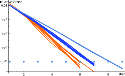
Figure 6: History of relative errors in BiCGStab. The data points at $L^{2}=16^{2}$ are joined by an orange line for each $w\in T_{z}{\mathbb{C}}^{N}$ randomly generated (with a fixed $z$), those at $L^{2}=128^{2}$ by a blue line, and those at $L^{2}=512^{2}$ by a gray line. We set the tolerance at $10^{-10}$.

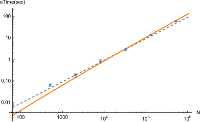
Figure 7: Elapsed time of the inversion of the linear problem $Aw_{0}=w$ with BiCGStab. The dashed gray line stands for $9\times 10^{-5}\times N$, and the solid orange line for $10^{-5}\times N\log N$.

Figure 8 is the elapsed time to solve eq. (3.37) with respect to $(u,\lambda)$ using the simplified Newton equation (Algorithm 1) for a given $(z,\pi)\in T\Sigma$. The physical and molecular dynamics parameters are the same as above. The iteration is terminated when $B\,(=z+\Delta z-\lambda-z_{\rm new})$ [eq. (3.40)] falls below a prescribed absolute tolerance $(=10^{-10})$. The statistical errors are estimated from ten $(z,\pi)$’s randomly generated in $T\Sigma$. This shows that the computational cost would be in the range $O(N)\sim O(N\,(\log N)^{2})$. The computational cost scaling is studied in more detail in a subsequent paper [33].

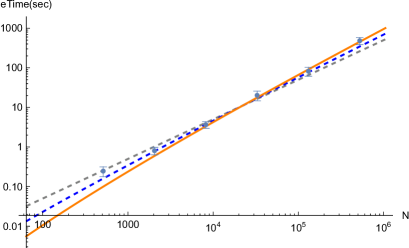
Figure 8: Elapsed time to solve eq. (3.37) with the simplified Newton equation (Algorithm 1). The dashed gray line stands for $5\times 10^{-4}\times N$, the dashed blue line for $5\times 10^{-5}\times N\log N$, and the solid orange line for $5\times 10^{-6}\times N\,(\log N)^{2}$.

6 Conclusion

We have developed a simplified algorithm for the GT-HMC and the WV-HMC methods, by adopting a simplified Newton method in determining the Lagrange multiplies of RATTLE iteratively. Using as a benchmark model the complex scalar field theory at finite density, we performed a numerical test for the convergence of the simplified Newton method. We found that the convergence depends on the system size only weakly and the cost of the RATTLE algorithm is nearly $O(N)$.

In subsequent papers [33, 34], we apply the current algorithm to various quantum field theories. The target models of the WV-HMC method can be classified into two categories. The first consists of models whose action is purely local, for which the Hessian $(H_{ij}=\partial_{i}\partial_{j}S)$ appearing in flow equations are sparse matrices. A typical example is the complex scalar field theory at finite density, and will be studied in [33]. The other treats the models whose bosonized actions include nonlocal terms such as the logarithm of the fermion determinant. A study of dynamical fermion systems with the WV-HMC method will be made in [34].

Models discussed above have configuration spaces of flat geometry. Actually, the WV-HMC method can also be generalized to models whose configuration spaces are group manifolds. This will be discussed in [35].

Besides applying the WV-HMC method to various models, we believe that it is also important to keep improving the algorithm itself. It should be interesting to combine the WV-HMC algorithm with other methods towards solving the sign problem, such as the complex Langevin method and/or the tensor network method. It is also interesting to incorporate machine learning techniques in order to further reduce the computational cost.

One of the most important projects in the near future is to develop the Monte Carlo algorithm to study the real-time dynamics of quantum many-body systems (see, e.g., [40, 41, 42, 43] for attempts based on the generalized thimble method). A study based on the WV-HMC is now in progress and will be reported elsewhere.

Appendix A Proof of eq. (4.25)

We start from the expression

$$\overline{\partial V}=\frac{1}{2}\,\overline{\partial S}+W^{\prime}(t)\,\overline{\partial t}=\frac{1}{2}\,\xi+W^{\prime}(t)\,\overline{\partial t}.$$ (A.1)

We decompose $\overline{\partial t}\in T_{z}{\mathbb{C}}^{N}$ at $z\in\Sigma_{t}\,(\subset{\mathcal{R}})$ into the form

$$\overline{\partial t}=(\overline{\partial t})_{\parallel}+(\overline{\partial t})_{\perp}=v+c\,\xi_{n}+(\overline{\partial t})_{\perp}$$ (A.2)

with $v=v^{a}E_{a}\in T_{z}\Sigma_{t}\,(\subset T_{z}{\mathcal{R}})$. Note that $\xi_{n}\in N_{z}\Sigma_{t}\cap T_{z}{\mathcal{R}}$ and $(\overline{\partial t})_{\perp}\in N_{z}{\mathcal{R}}$. In the following, we will show that (1) $v=0$ and (2) $c=1/(2\,\langle\xi_{n},\xi_{n}\rangle)$. This completes the proof because $(\overline{\partial t})_{\perp}\in N_{z}{\mathcal{R}}$ can be absorbed into $\lambda$ in (4.22).

(1) For $\forall z\in\Sigma_{t}$, $\forall u=u^{a}E_{a}\in T_{z}\Sigma_{t}$ and an infinitesimally small $\epsilon$, we have

$$t(z,\bar{z})=t(z+\epsilon u,\bar{z}+\epsilon\bar{u})=t(z,\bar{z})+\epsilon\,[u^{i}\,\partial_{i}t+\overline{u^{i}}\,\overline{\partial_{i}t}]+O(\epsilon^{2}),$$ (A.3)

and thus,

$$0=u^{i}\,\partial_{i}t+\overline{u^{i}}\,\overline{\partial_{i}t}=2\,\langle u,\overline{\partial t}\rangle=2\,\langle u,v\rangle=2\,u^{a}\gamma_{ab}v^{b}.$$ (A.4)

This means that $v=0$ due to the nondegeneracy of $\gamma_{ab}$.

(2) By using the orthogonality, $c$ is given by

$$c=\frac{\langle\xi_{n},\overline{\partial t}\rangle}{\langle\xi_{n},\xi_{n}\rangle}.$$ (A.5)

Here, noting that

$$1=[t(z,\bar{z})]^{\centerdot}=\dot{z}^{i}\,\partial_{i}t+\overline{\dot{z}^{i}}\,\overline{\partial_{i}t}=\xi^{i}\,\partial_{i}t+\overline{\xi^{i}}\,\overline{\partial_{i}t}=2\,\langle\xi,\overline{\partial t}\rangle=2\,\langle\xi_{n},\overline{\partial t}\rangle\quad(\because v=0),$$ (A.6)

we have $\langle\xi_{n},\overline{\partial t}\rangle=1/2$. We thus obtain $c=1/(2\,\langle\xi_{n},\xi_{n}\rangle)$.

References

- [1] G. Aarts, Introductory lectures on lattice QCD at nonzero baryon number. J. Phys. Conf. Ser. 706, no. 2, 022004 (2016) [arXiv:1512.05145 [hep-lat]].
- [2] L. Pollet, Recent developments in Quantum Monte-Carlo simulations with applications for cold gases, Rep. Prog. Phys. 75, 094501 (2012) [arXiv:1206.0781 [cond-mat.quant-gas]].
- [3] G. Parisi, “On complex probabilities,” Phys. Lett. B 131, 393 (1983).
- [4] J.R. Klauder, “Coherent State Langevin Equations for Canonical Quantum Systems With Applications to the Quantized Hall Effect,” Phys. Rev. A 29, 2036 (1984).
- [5] G. Aarts, “Can stochastic quantization evade the sign problem? The relativistic Bose gas at finite chemical potential,” Phys. Rev. Lett. 102, 131601 (2009) [arXiv:0810.2089 [hep-lat]].
- [6] G. Aarts, E. Seiler and I. O. Stamatescu, “The Complex Langevin method: When can it be trusted?,” Phys. Rev. D 81, 054508 (2010) [arXiv:0912.3360 [hep-lat]].
- [7] G. Aarts, F. A. James, E. Seiler and I. O. Stamatescu, “Complex Langevin: Etiology and Diagnostics of its Main Problem,” Eur. Phys. J. C 71, 1756 (2011) [arXiv:1101.3270 [hep-lat]].
- [8] K. Nagata, J. Nishimura and S. Shimasaki, “Argument for justification of the complex Langevin method and the condition for correct convergence,” Phys. Rev. D 94, no.11, 114515 (2016) [arXiv:1606.07627 [hep-lat]].
- [9] E. Witten, “Analytic continuation of Chern-Simons theory,” AMS/IP Stud. Adv. Math. 50, 347-446 (2011) [arXiv:1001.2933 [hep-th]].
- [10] M. Cristoforetti, F. Di Renzo and L. Scorzato, “New approach to the sign problem in quantum field theories: High density QCD on a Lefschetz thimble,” Phys. Rev. D 86, 074506 (2012) [arXiv:1205.3996 [hep-lat]].
- [11] M. Cristoforetti, F. Di Renzo, A. Mukherjee and L. Scorzato, “Monte Carlo simulations on the Lefschetz thimble: Taming the sign problem,” Phys. Rev. D 88, no. 5, 051501(R) (2013) [arXiv:1303.7204 [hep-lat]].
- [12] H. Fujii, D. Honda, M. Kato, Y. Kikukawa, S. Komatsu and T. Sano, “Hybrid Monte Carlo on Lefschetz thimbles - A study of the residual sign problem,” JHEP 1310, 147 (2013) [arXiv:1309.4371 [hep-lat]].
- [13] H. Fujii, S. Kamata and Y. Kikukawa, “Lefschetz thimble structure in one-dimensional lattice Thirring model at finite density,” JHEP 11, 078 (2015) [erratum: JHEP 02, 036 (2016)] [arXiv:1509.08176 [hep-lat]].
- [14] H. Fujii, S. Kamata and Y. Kikukawa, “Monte Carlo study of Lefschetz thimble structure in one-dimensional Thirring model at finite density,” JHEP 12, 125 (2015) [erratum: JHEP 09, 172 (2016)] [arXiv:1509.09141 [hep-lat]].
- [15] A. Alexandru, G. Başar and P. Bedaque, “Monte Carlo algorithm for simulating fermions on Lefschetz thimbles,” Phys. Rev. D 93, no. 1, 014504 (2016) [arXiv:1510.03258 [hep-lat]].
- [16] A. Alexandru, G. Başar, P. F. Bedaque, G. W. Ridgway and N. C. Warrington, “Sign problem and Monte Carlo calculations beyond Lefschetz thimbles,” JHEP 1605, 053 (2016) [arXiv:1512.08764 [hep-lat]].
- [17] M. Fukuma and N. Umeda, “Parallel tempering algorithm for integration over Lefschetz thimbles,” PTEP 2017, no. 7, 073B01 (2017) [arXiv:1703.00861 [hep-lat]].
- [18] A. Alexandru, G. Başar, P. F. Bedaque and N. C. Warrington, “Tempered transitions between thimbles,” Phys. Rev. D 96, no. 3, 034513 (2017) [arXiv:1703.02414 [hep-lat]].
- [19] M. Fukuma, N. Matsumoto and N. Umeda, “Applying the tempered Lefschetz thimble method to the Hubbard model away from half filling,” Phys. Rev. D 100, no. 11, 114510 (2019) [arXiv:1906.04243 [cond-mat.str-el]].
- [20] A. Alexandru, “Improved algorithms for generalized thimble method,” talk at the 37th international conference on lattice field theory, Wuhan, 2019.
- [21] M. Fukuma, N. Matsumoto and N. Umeda, “Implementation of the HMC algorithm on the tempered Lefschetz thimble method,” [arXiv:1912.13303 [hep-lat]].
- [22] M. Fukuma and N. Matsumoto, “Worldvolume approach to the tempered Lefschetz thimble method,” PTEP 2021, no.2, 023B08 (2021) [arXiv:2012.08468 [hep-lat]].
- [23] M. Fukuma, N. Matsumoto and Y. Namekawa, “Statistical analysis method for the worldvolume hybrid Monte Carlo algorithm,” PTEP 2021, no.12, 123B02 (2021) [arXiv:2107.06858 [hep-lat]].
- [24] Y. Mori, K. Kashiwa and A. Ohnishi, “Toward solving the sign problem with path optimization method,” Phys. Rev. D 96, no.11, 111501 (2017) [arXiv:1705.05605 [hep-lat]].
- [25] Y. Mori, K. Kashiwa and A. Ohnishi, “Application of a neural network to the sign problem via the path optimization method,” PTEP 2018, no.2, 023B04 (2018) [arXiv:1709.03208 [hep-lat]].
- [26] A. Alexandru, P. F. Bedaque, H. Lamm and S. Lawrence, “Finite-Density Monte Carlo Calculations on Sign-Optimized Manifolds,” Phys. Rev. D 97, no.9, 094510 (2018) [arXiv:1804.00697 [hep-lat]].
- [27] F. Bursa and M. Kroyter, “A simple approach towards the sign problem using path optimisation,” JHEP 12, 054 (2018) [arXiv:1805.04941 [hep-lat]].
- [28] M. Levin and C. P. Nave, “Tensor renormalization group approach to 2D classical lattice models,” Phys. Rev. Lett. 99, 120601 (2007) [arXiv:cond-mat/0611687 [cond-mat.stat-mech]].
- [29] Z.Y. Xie et al., “Coarse-graining renormalization by higher-order singular value decomposition,” Phys. Rev. B 86, 045139 (2012) [arXiv:1201.1144 [cond-mat.stat-mech]].
- [30] D. Adachi, T. Okubo and S. Todo, “Anisotropic Tensor Renormalization Group,” Phys. Rev. B 102, no.5, 054432 (2020) [arXiv:1906.02007 [cond-mat.stat-mech]].
- [31] Y. Shimizu and Y. Kuramashi, “Grassmann tensor renormalization group approach to one-flavor lattice Schwinger model,” Phys. Rev. D 90, no.1, 014508 (2014) [arXiv:1403.0642 [hep-lat]].
- [32] S. Akiyama and D. Kadoh, “More about the Grassmann tensor renormalization group,” JHEP 10, 188 (2021) [arXiv:2005.07570 [hep-lat]].
- [33] M. Fukuma and Y. Namekawa, “Applying the Worldvolume Hybrid Monte Carlo method to the complex scalar field theory at finite density,” in preparation.
- [34] M. Fukuma and Y. Namekawa, “Applying the Worldvolume Hybrid Monte Carlo method to dynamical fermion systems,” in preparation.
- [35] M. Fukuma, “Worldvolume Hybrid Monte Carlo algorithm for group manifolds,” in preparation.
- [36] H. C. Andersen, “RATTLE: A “velocity” version of the SHAKE algorithm for molecular dynamics calculations,” J. Comput. Phys. 52, 24 (1983).
- [37] B. J. Leimkuhler and R. D. Skeel, “Symplectic numerical integrators in constrained Hamiltonian systems,” J. Comput. Phys. 112, 117 (1994).
- [38] M. Cristoforetti, F. Di Renzo, G. Eruzzi, A. Mukherjee, C. Schmidt, L. Scorzato and C. Torrero, “An efficient method to compute the residual phase on a Lefschetz thimble,” Phys. Rev. D 89, no.11, 114505 (2014) [arXiv:1403.5637 [hep-lat]].
- [39] E. Hairer, S. P. Nørsett, G. Wanner, “Solving Ordinary Differential Equations I,” Springer Series in Computational Mathematics 8, Springer (2009).
- [40] A. Alexandru, G. Basar, P. F. Bedaque, S. Vartak and N. C. Warrington, “Monte Carlo Study of Real Time Dynamics on the Lattice,” Phys. Rev. Lett. 117, no.8, 081602 (2016) [arXiv:1605.08040 [hep-lat]].
- [41] Z. G. Mou, P. M. Saffin, A. Tranberg and S. Woodward, “Real-time quantum dynamics, path integrals and the method of thimbles,” JHEP 06, 094 (2019) [arXiv:1902.09147 [hep-lat]].
- [42] Z. G. Mou, P. M. Saffin and A. Tranberg, “Quantum tunnelling, real-time dynamics and Picard-Lefschetz thimbles,” JHEP 11, 135 (2019) [arXiv:1909.02488 [hep-th]].
- [43] J. Nishimura, K. Sakai and A. Yosprakob, “A new picture of quantum tunneling in the real-time path integral from Lefschetz thimble calculations,” JHEP 09, 110 (2023) [arXiv:2307.11199 [hep-th]].