Aging Dynamics of $d-$dimensional Locally Activated Random Walks

Abstract

Locally activated random walks are defined as random processes, whose dynamical parameters are modified upon visits to given activation sites. Such dynamics naturally emerge in living systems as varied as immune and cancer cells interacting with spatial heterogeneities in tissues, or at larger scales animals encountering local resources. At the theoretical level, these random walks provide an explicit construction of strongly non Markovian, and aging dynamics. We propose a general analytical framework to determine various statistical properties characterizing the position and dynamical parameters of the random walker on $d$-dimensional lattices. Our analysis applies in particular to both passive (diffusive) and active (run and tumble) dynamics, and quantifies the aging dynamics and potential trapping of the random walker; it finally identifies clear signatures of activated dynamics for potential use in experimental data.

Locally activated random walks (LARWs) are defined as stochastic processes that undergo changes in their dynamic characteristics when they encounter specific sites, called hereafter activation sites [1, 2, 3]. Such locally activated dynamics, where activation sites either accelerate or slow down the process, can be typically observed in living systems, such as cells navigating through tissues [4, 5], or on a larger scale, when animals exploit local resources, or on the contrary visit infected areas [6, 7]. For example, it has been observed that immune (dendritic) cells, whose function is to collect chemical signals (antigens) left by pathogens, switch from a slow, non persistent state, to a fast and persistent state, which eventually helps triggering the specific immune response [4]. This switch occurs when a threshold amount of chemical signals has been collected, after many visits to antigen concentrated spots; the switch can also occur in absence of infection signals, when the cells have been mechanically confined, as happens when they randomly migrate through tight pores distributed throughout tissues [8].

At the theoretical level, a minimal description of such dynamics suggests to endow the random walker (RWer) of interest, whose position at time $t$ will be hereafter denoted by $x(t)$, with an internal scalar variable $a(t)$ – called activation hereafter –, which is a random variable controlled by the history of successive visits of the RWer to given activation sites up to $t$. In turn it is posited that the parameters ruling the dynamics of the RWer, typically its instantaneous speed or persistence, depend on $a$. This minimal choice makes the dynamics of the position $x(t)$ of a LARWer genuinely non Markovian, because it depends on the past trajectory $\{x(t^{\prime})\}_{t^{\prime}\leq t}$, and aging, because the statistics of the activation $a(t)$ is typically non stationary, eg depends on the observation time. Beyond the applications mentioned above, the class of LARWs thus provides an explicit microscopic construction of non Markovian, aging stochastic processes with a broad range of adjustable dynamic and geometric properties, which, as we show below, can be quantified analytically. Related examples of non-Markovian RWs, in which the memory of the complete past trajectory determines the future evolution, comprise self-avoiding walks [9], true self-avoiding walkers [10, 10, 11, 12], self-interacting RWs [13, 14, 15, 1, 16, 17, 18, 19, 20] and RWs with reinforcement such as the elephant walks [21, 22, 23].

So far, the analysis of LARWs has been restricted to the example of $1d$ Brownian dynamics, with a point like activation site [2]. Because a given point in space is almost surely never visited by a Brownian RWer for $d\geq 2$, this early analysis is not suitable to generalizations to higher space dimensions, which are of obvious importance for practical applications. In addition, this model was limited to Brownian motion and thus parametrized by a single parameter – the diffusion coefficient $D(a)$. It thus does not cover the case of persistent RWs – typically parametrized by both their instantaneous speed and persistence, which are paradigmatic models of active particles, required in particular in the description of living systems as exemplified above, be them cells or animals [24].

In what follows, we introduce a general $d$-dimensional lattice model of continuous time LARWs, which covers the case of both simple symmetric (Polya) and persistent RWs, with either accelerated or decelerated dynamics. We present a general framework to obtain exact, analytical determinations of the joint distribution $P(x,a,t)$ of the position and activation of the RWer at time $t$, which fully characterizes the process. Our analysis shows quantitatively that activation, even if localized at a single site, can deeply impact the dynamics at large scales. For generic accelerated processes, we show that the marginal distribution of the position of the RWer (denoted $P(x,t)$ for simplicity) is non Gaussian for $d=1,2,3$ – thereby generalizing the result of [2] obtained for $1d$ Brownian LARW. In contrast to the $1d$ case, which leads to anomalous diffusion, we find for $d=2,3$ a diffusive scaling $x\sim t^{1/2}$ for all choices of activation dynamics. For decelerated processes, we identify and characterize quantitatively a transition between a Gaussian, diffusive regime and a phase where the RWer can be irreversibly trapped at the activation site.

LARW : general framework.

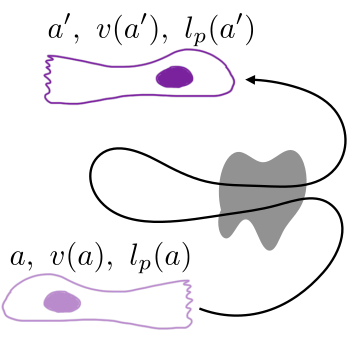
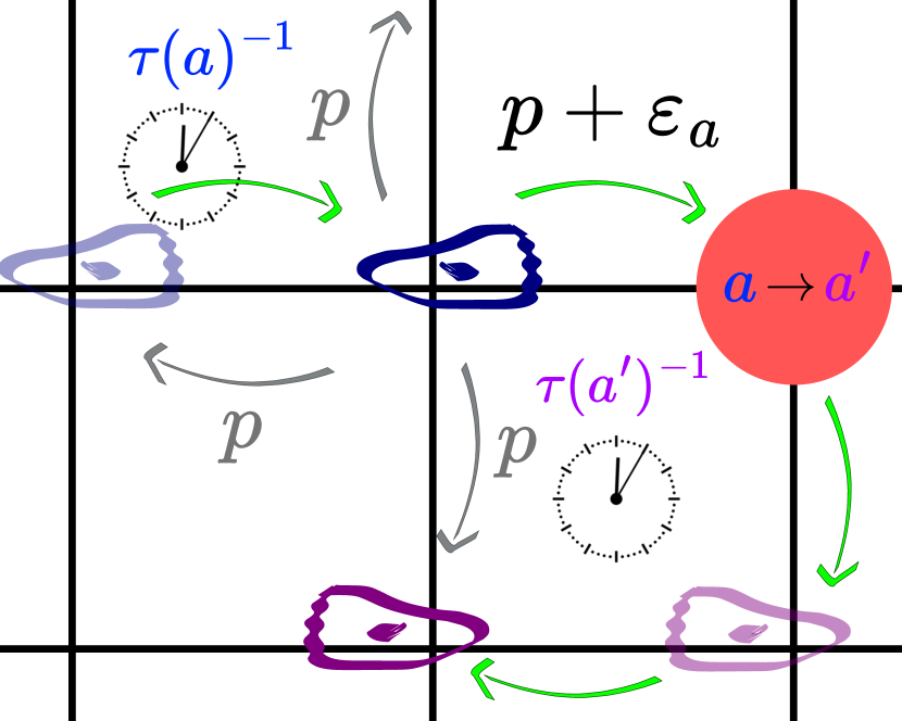
Figure 1: Left: Sketch of a LARWer (eg immune cell), whose dynamic parameters (speed $v$ and persistence length $l_{p}$) depend on the activation time $a$, which increases upon each visit to the activation site (eg antigen carrying site). Right: A persistent LARW on a 2D square lattice, with persistence parameter $\varepsilon_{a}$ ($p=\frac{1-\varepsilon_{a}}{4}$) and waiting time $\tau(a)$. The trajectory of the RWer is represented by the green arrows, and the activation site is represented by the red disk. The activation time increases from $a$ to $a^{\prime}$ upon the visit of the activation site.

We consider a RWer that performs a generic continuous time RW on a regular $d$-dimensional infinite lattice. More precisely, the RWer, if at site $s$ with activation time $a$, performs a jump with rate $1/\tau(a)$ to a site drawn from a given distribution (see explicit examples below and Fig. 1). The walk starts with activation time $a=0$ from the origin $x=0$, which is assumed by convention to be the only activation site of the lattice. In what follows, we assume that the activation $a$ of the RWer is only increasing and given by the cumulative time spent on the activation site up to time $t$, so that $a(t)=\int_{0}^{t}\mathds{1}\left(x(t^{\prime})\right)dt^{\prime}$, where $\mathds{1}\left(s\right)=1$ if $s$ is the activation site and 0 otherwise; in turn, $\tau(a)$ is a system dependent modelling choice, and can capture both accelerated (decreasing $\tau(a)$) and decelerated (increasing $\tau(a)$) processes. Of note, the aging dynamics of $a$ makes the position process $x(t)$ non Markovian, because the jump rate of the RW depends explicitly on the activation time $a$ that is controlled by the full history of visits of the RWer to the activation site. Nonetheless, the process $(x(t),a(t))$ is Markovian, and the joint distribution $P(x,a,t)$ fully characterizes the process ; we denote $\hat{P}(x,a,s)=\int_{0}^{\infty}e^{-st}P(x,a,t)dt$ its Laplace transform.

In what follows, we first show that even if $a(t)$ alone is not a markovian process, an explicit evolution equation for $P(0,a,t)$ can be obtained. Writing $P(0,t+dt,a+dt)$ as a partition over the last time the hotspot was visited yields two different scenarii : (i) the walker was at $0$ at time $t$ with activation time $a$ and did not jump during $dt$, or (ii) the walker jumped from $0$ at an earlier time $t^{\prime}<t$ with activation time $a+dt$ and came back exactly at $t+dt$. The key point is that between two consecutive visits to the activation site, the activation time $a$, and thus the jump rate $1/\tau(a)$ of the RWer remains constant. Thus, the probability of events involved in (ii) can be written in terms of the first-passage time (FPT) density to site $0$ for a simple random walker with constant jump rate $1/\tau(a)$ starting from a neighboring site of $0$, which is denoted $F_{a}(0|\partial_{0},t)$. This yields (see supplementary material (SM) for details)

$$\begin{gathered}\partial_{t}P(0,a,t)+\partial_{a}P(0,a,t)=\\ -\frac{P(0,a,t)}{\tau(a)}+\int_{0}^{t}\frac{dt^{\prime}}{\tau(a)}P(0,a,t^{\prime})F_{a}(0|\partial_{0},t-t^{\prime}).\end{gathered}$$ (1)

Next, we define $\xi_{a}(s)=(1+s\tau(a))^{-1}$ and Laplace-transform (1) to obtain a first important result

$$\partial_{a}\hat{P}(0,a,s)=\frac{[\mathcal{F}\big{(}0|0,\xi_{a}(s)\big{)}-1]\hat{P}(0,a,s)}{\tau(a)\xi_{a}(s)}$$ (2)

where we introduced the discrete-time, non-activated first-passage generating function $\mathcal{F}(0|0,\xi)$, related to its continuous-time, activated counterpart $\hat{F}_{a}(0|\partial_{0},s)$ by $\hat{F}_{a}(0|\partial_{0},s)=\mathcal{F}(0|0,\xi_{a}(s))/\xi_{a}(s)$ [9]. Integrating this equation is straightforward and yields an explicit expression for $\hat{P}(0,a,s)$, provided that $\mathcal{F}(0|0,\xi)$ is known.

We now show how to obtain the full joint distribution $P(x,a,t)$ from (2). For the walker to be on site $x$ with activation $a$ at $t$, it must jump away from $0$ at an earlier time $t^{\prime}$ with activation $a$, and next reach site $x$ without hitting $0$ in the remaining time $t-t^{\prime}$. This analysis yields the following renewal equation

$$P(x,a,t)=\int_{0}^{t}\frac{dt^{\prime}}{\tau(a)}P(0,a,t^{\prime})P^{a}_{\text{surv}}(x|\partial_{0},t-t^{\prime})$$ (3)

where we define $P^{a}_{\text{surv}}(x|\partial_{0},t)$ to be the (survival) probability for a walker with activation $a$, starting from site $0$ and jumping at time $0^{+}$, to be at site $x$ at time $t$, all this without visiting site $0$ again. This quantity is related [9] to its non-activated, discrete-time counterpart $\mathcal{P}_{\text{surv}}(x|0,\xi)$ by $\hat{P}^{a}_{\text{surv}}(x|\partial_{0},s)=\tau(a)\xi_{a}(s)\frac{\mathcal{P}_{\text{surv}}(x|0,\xi_{a}(s))}{\xi_{a}(s)}$. The Laplace transform of (3) thus yields

$$\hat{P}(x,a,s)=\hat{P}(0,a,s)\mathcal{P}_{\text{surv}}(x|0,\xi_{a}(s)).$$ (4)

We now recall how all the quantities entering (2), (4) can be deduced from the generating function $\mathcal{P}(x|y,\xi)$ of the propagator of the corresponding non activated RW. Standard results [9] yield the discrete-time generating function $\mathcal{P}_{\text{surv}}(x|0,\xi)$

$$\mathcal{P}_{\text{surv}}(x|0,\xi)=\mathcal{F}(x|0,\xi)=\frac{\mathcal{P}(x|0,\xi)}{\mathcal{P}(0|0,\xi)}$$ (5)

as well as the first-return time to $0$

$$\mathcal{F}(0|0,\xi)=1-\frac{1}{\mathcal{P}(0|0,\xi)}.$$ (6)

Using these results, one finds finally the exact expression of the Laplace transformed joint law

$$\hat{P}(x,a,s)=\frac{\mathcal{P}(x|0,\xi_{a})}{\mathcal{P}(0|0,\xi_{a})}\exp\left(-\int_{0}^{a}\frac{db}{\tau(b)\xi_{b}\mathcal{P}(0|0,\xi_{b})}\right).$$ (7)

We stress that this determination of the joint law is fully explicit for all processes for which the propagator of the underlying, non activated RW is known. We present explicit examples below.

$d$-dimensional nearest neighbor LARWs. For the paradigmatic example of symmetric nearest neighbor RWs on the hypercubic lattice $\mathbb{Z}^{d}$, one has the following integral representation of the (non activated) propagator [9]:

$$\mathcal{P}\left(x=(x_{k})_{k=1\dots d},\xi\right)=\int_{0}^{\infty}e^{-u}\prod_{k=1}^{d}I_{x_{k}}\left(\frac{u\xi}{d}\right)du$$ (8)

where $I_{x_{k}}$ is a modified Bessel function.

For $d=1$, making use of Eq.7 yields (see SM):

$$\hat{P}_{1D}(x,a,s)=\left(\frac{1-\sqrt{1-\xi_{a}^{2}}}{\xi_{a}}\right)^{|x|}\exp\left(-\int_{0}^{a}\frac{db}{\tau(b)}\frac{\sqrt{1-\xi_{b}^{2}}}{\xi_{b}}\right)$$ (9)

While this expression cannot, to the best of our knowledge, be Laplace inverted analytically for arbitrary $\tau(a)$, numerical inversion is straightforward and provides the joint law at all times. Under the condition that $\tau(a)\ll a$ for $a\to\infty$ (to be refined below), a smooth (non singular) continuous limit, defined by $x\to\infty,x^{2}\tau(a)/t$ fixed, can be obtained and yields the following asymptotic expression of the joint law of $x,a$

$$P_{1D}(x,a,t)\sim\frac{Ze^{-\frac{Z^{2}}{2t}}}{\sqrt{2\pi}t^{3/2}}$$ (10)

where $Z=\sqrt{\tau(a)}|x|+F_{1}(a),F_{1}(a)=\int_{0}^{a}\frac{db}{\sqrt{\tau(b)}}$. In turn, considering the explicit example of $\tau(a)\sim a^{-\alpha}$ with $\alpha>-1$ (to ensure $\tau(a)\ll a$ for $a\to\infty$), integration over $a$ using the saddle point method yields the marginal distribution

$$P_{1D}(x,t)\sim\begin{cases}A(\alpha)\frac{x^{\frac{1}{1+\alpha}}}{t}\exp(-B(\alpha)\frac{x^{\frac{2+\alpha}{1+\alpha}}}{4t}),\alpha>0\\ \frac{e^{-\frac{x^{2}}{2t}}}{\sqrt{2\pi t}(1-\frac{\alpha}{2}|x|)},-1<\alpha<0\end{cases}$$ (11)

where $A,B$ are constants explicitly given in SM. Of note, the marginal distribution is thus non Gaussian, and even non monotonic as a function of $x$ in the case of accelerated processes. These results generalize the earlier findings of [2], where a similar $1d$ model of LARW for a Brownian particle in continuous space, with a pointlike activation site was studied. These earlier results are indeed recovered by taking the appropriate continuous limit of (10),(11) (see SM).

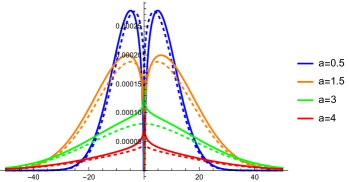
Figure 2: Joint law of activation time (colors) and position (abscissa, along a given axis) of an accelerating 2D LARW with waiting time $\tau(a)=\frac{1}{a}$. Thick lines are obtained from numerical Laplace inversion of (12), while dashed lines correspond to the asymptotics (13).

We now turn to LARW on the 2–dimensional square lattice. Using (7),(8), the joint law of $x=(x_{1},x_{2})$ and $a$ can be written in Laplace space

$$\hat{P}_{2D}(x,a,s)= \frac{\pi\int_{0}^{\infty}e^{-u}I_{x_{1}}\left(\frac{\xi_{a}u}{2}\right)I_{x_{2}}\left(\frac{\xi_{a}u}{2}\right)du}{2K(\xi_{a}^{2})}$$ (12)

$$\times\exp\left(-\frac{\pi}{2}\int_{0}^{a}\frac{db}{\tau(b)\xi_{b}K(\xi_{b}^{2})}\right)$$

where $K$ is the elliptic integral. While there is a priori no simple Laplace inversion of this expression, numerical inversion can be performed and provides the joint law for all values of parameters (see Fig 2).

In addition, in the scaling regime $x\to\infty,x^{2}\tau(a)/t$ fixed, Laplace inversion can be performed analytically (assuming $\tau(a)\ll a$ for $a\to\infty$, see SM) and yields :

$$P_{2D}(x,a,t)\sim-\frac{\tau(a)}{\pi t}e^{-\frac{|x|^{2}\tau(a)}{t}}\partial_{a}e^{-\frac{\pi F_{2}(a)}{\log\frac{8t^{2}}{\tau(a)^{2}|x|^{2}}}}$$ (13)

where $F_{2}(a)=\int_{0}^{a}\frac{db}{\tau(b)}$. This expression of the joint law is found to be in very good agreement with the numerical inversion (see Fig 2). Of note, different behaviours are obtained according to the value of $a$ relative to a threshold value $a_{*}(t)$, which can be determined from the analysis of (13), and turns out to scale as the typical value of $a$ at time $t$ (see SM) . For $a<a_{*}$, trajectories with atypically low numbers of visits to the activation site are selected. This leads to an effective repulsion from the activation site, so that $P_{2D}(x,a,t)$ as a function of $x$ displays a local minimum for $x=(0,0)$. Conversely, for $a>a_{*}$, trajectories with atypically large numbers of visits to the activation site are selected, and $P_{2D}(x,a,t)$ shows a sharp maximum for $x=(0,0)$.

We now turn to the determination of the marginal distribution of the position at time $t$. To be explicit, we consider the example $\tau(a)\sim\frac{1}{a^{\alpha}}$ with $\alpha>-1$ (to ensure $\tau(a)\ll a$ for $a\to\infty$). Using again the saddle point method in the regime $x/\sqrt{t}\gg 1$, one finds, up to subleading $\log\log$ corrections:

$$P_{2D}(x,t)\sim\begin{cases}\frac{A(\alpha)}{t}(\frac{x}{\sqrt{t}})^{\frac{1-\alpha}{2\alpha+1}}e^{-\frac{B(\alpha)(\frac{x^{2}}{t})^{\frac{1+\alpha}{1+2\alpha}}}{\log^{\frac{\alpha}{1+2\alpha}}\left(C(\alpha)\left(\frac{t^{1+\alpha}}{x}\right)^{\frac{1}{1+2\alpha}}\right)}},\alpha>0\\ \frac{\exp(-\frac{x^{2}}{t})}{t\left(\pi-\frac{\alpha x^{2}}{t}\log\left(\frac{8t^{2}}{x^{2}}\right)\right)},-1<\alpha<0\end{cases}$$ (14)

where $A$ is a slowly varying function of $x$ and $t$, and $B,C$ are constants, which are explicitly given in SM. This analytical expression of the distribution, confirmed by numerical simulations, is strongly non-Gaussian, similarly to the $1d$ case (see Fig.3). In addition, for accelerated processes ($\alpha>0$), this distribution is maximized for a non vanishing, increasing in time displacement $r_{*}(t)$.

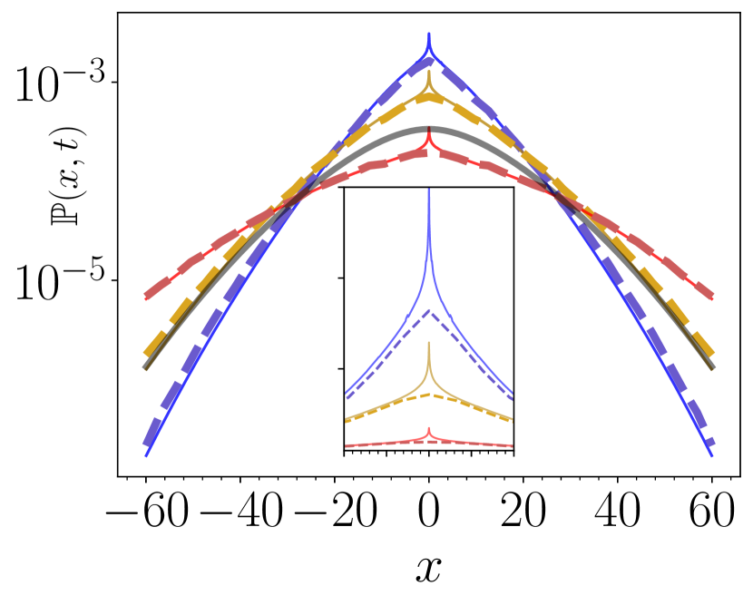
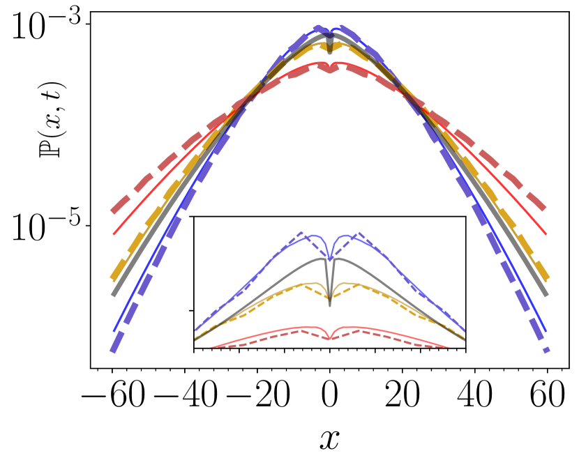
Figure 3: Spatial distribution for a persistent 2D LARW with a single hotspot at the origin with persistence parameter $\varepsilon$, along a given axis $x$. Blue, yellow and red curves correspond respectively to $\varepsilon=-0.3,0,0.4$. Black lines correspond to the saddle-point approximations (14) and are drawn for $\varepsilon=0$. Thick lines are obtained from numerical integration over $a$ of the asymptotic expression (13) with rescaled waiting time $\tilde{\tau}(a)=\frac{1-\varepsilon}{1+\varepsilon}\tau(a)$, while dashed lines correspond to numerical simulations. (a) Decelerating LARW, with $\tau(a)=\sqrt{1+a}$. Note the cusp at site $x=0$. (b) Accelerating LARW, with $\tau(a)=\frac{1}{a}$. Note the nonzero typical displacement scaling logarithmically with time.

We now turn to LARW on the $3d$ cubic lattice. As opposed to the above $d=1,2$ cases, the $3d$ non activated RW is known to be transient, so that $P(0|0,\xi_{a})$ tends to the finite value $\frac{1}{1-R}$ as $as\ll 1$, where $R\simeq 0.34...$ is the return probability on the cubic lattice [9]. This allows for an explicit Laplace inversion in the regime $x\to\infty,a\ll t,x^{2}\tau(a)/t$ fixed, which yields using (7) (assuming $\tau(a)\ll a$ for $a\to\infty$):

$$P_{3D}(x,a,t)\sim(1-R)\sqrt{\tau(a)}\bigg{(}\frac{3}{2\pi t}\bigg{)}^{3/2}$$ (15)

$$\times\exp(-\frac{3|x|^{2}\tau(a)}{2t}-(1-R)F_{3}(a))$$

where $F_{3}(a)=\int_{0}^{a}\frac{db}{\tau(b)}$. Of note, in contrast to the case of recurrent RWs for $d=1,2$, (15) is a Gaussian function of $x$ (for $a$ fixed), and is maximized at the origin, and this regardless of $\tau(a)$, for both accelerated and decelerated processes. Finally, taking the example of $\tau(a)\sim 1/a^{\alpha}$, the marginal distribution of the position is obtained by saddle-point integration of (15) in the regime $x/\sqrt{t}\gg 1$

$$P_{3D}(x,t)\sim\begin{cases}\frac{A(\alpha)}{t^{3/2}}\left(\frac{x}{\sqrt{t}}\right)^{\frac{1-2\alpha}{1+2\alpha}}e^{-B(\alpha)\left(\frac{x^{2}}{t}\right)^{\frac{1+\alpha}{1+2\alpha}}},\alpha>0\\ \left(\frac{3}{2\pi t}\right)^{3/2}\frac{e^{-\frac{3x^{2}}{2t}}}{1-\frac{3\alpha x^{2}}{2t(1-R)}},-1<\alpha<0\end{cases}$$ (16)

where $A(\alpha),B(\alpha)$ are constants and are given explicitly in the SM. Of note this distribution shows a diffusive scaling $x^{2}\propto t$, even if non Gaussian. Therefore, a localized perturbation by a single activation site, even for a transient RW that typically makes only a finite number of visits to this site, is sufficient to yield a non Gaussian behaviour.

Persistent (active) LARWs. Last, we show that (2) can in fact be used beyond the case of symmetric nearest neighbor RWs. For the sake of simplicity, we consider a $1d$ RWer that performs a persistent RW on $\mathbb{Z}$ [26], which is the discrete space analog of the classical run and tumble model of active particle. Our results below can be generalized to $d$-dimensional persistent RWs as shown in SM. In this model, after a jump $\sigma=\pm 1$, the walker performs an identical jump $\sigma$ with probability $\frac{1+\varepsilon}{2}$, and $-\sigma$ with probability $\frac{1-\varepsilon}{2}$. Local activation is taken into account by allowing both the jump rate $1/\tau(a)$ and the persistence parameter $\varepsilon_{a}\in[-1,1]$ to depend on activation $a$, whose definition is unchanged. Eq. (4) remains valid for this process, and yields the Laplace transform of the joint distribution $\hat{P}(x\neq 0,a,s)$, given in Eq.(9) of the SM. Importantly, this expression, upon numerical inversion, gives access to the joint law at all times. In addition the $as\ll 1$ asymptotics of this equation show that at large scales the persistent LARW can be mapped exactly to a non-persistent nearest neighbor LARW with rescaled waiting time $\tilde{\tau}(a)=\frac{1-\varepsilon(a)}{1+\varepsilon(a)}\tau(a)$, for which explicit expressions of the joint law have been obtained above. This result holds in any space dimension, and explicitly quantifies how the activation of either persistence ($\varepsilon(a)$) or velocity ($1/\tau(a)$) impacts on the large scale dynamics of the process. In particular, acceleration ($\tilde{\tau}(a)\to 0$) can be achieved either by increasing the instantaneous speed ($\tau(a)\to 0$) or increasing persistence ($\varepsilon(a)\to 1$), as quantified by our approach.

Ergodicity breaking and trapping. In the case of decelerated processes, the particle can eventually be trapped at the activation site. Quantitatively, this trapping occurs if the particle asymptotically spends a finite fraction of time at 0, so that there is some $\gamma>0$ such that $\lim_{t\to\infty}P(0,a=\gamma t,t)>0$ and the joint law is non smooth (singular) at large times. The analysis of the joint law (7) shows (see SM) that such ergodicity breaking occurs if and only if

$$S\equiv e^{-\int_{0}^{\infty}\frac{da}{\tau(a)}}>0.$$ (17)

Of note, this condition holds in all space dimensions; in the example $\tau(a)\sim a^{-\alpha}$ discussed above this occurs for $\alpha<-1$. This condition of trapping is also realised if $\tau(a)$ diverges for a finite activation $a_{f}$. Importantly, while general expressions (9), (12) of the joint law are valid for both trapping and non trapping regimes, explicit expressions (11), (13), (14), (16) have been obtained in the ergodic regime $S=0$ (or more loosely $\tau(a)\ll a$), and thus remain smooth. In the case of nearest neighbor RWs, the trapping condition (17) amounts to requiring that the probability $S$ that the walker remains on the activation site forever upon a given visit is non vanishing. In turn, for persistent RWs this condition applies to the effective $\tilde{\tau}$, and reveals two possible mechanisms for trapping: either waiting times diverge ($\tau(a)\to\infty)$, as in the case of trapped nearest neighbor RWs, or the RW becomes infinitely antipersistent ($\varepsilon(a)\to-1)$. Our analysis allows to quantify asymptotically in the large $t$ regime the dynamics of trapping by considering $P(0,a=\gamma t,t)$ in the large $t$ regime, which is obtained from the $s\to 0$ behaviour of $\hat{P}(0,a=\gamma/s,s)$ in the non-ergodic regime (see SM). This shows that for $d=1,2$, ie recurrent RWs, $P(0,a,t)\sim(1-w_{d}(t))\delta(a-\gamma t)$, where $\gamma=1$ for simple and persistent LARWs with $\tau(a)\to\infty$ and $\gamma=1/2$ for persistent LARWs with $\varepsilon(a)\to-1$. The weight $w_{d}(t)$ is given explicitly in SM and vanishes for $t\to\infty$, so that the RWer is eventually trapped with probability 1. For $d=3$, ie transient RWs, one has $P(0,a,t)\sim e^{-(1-R)\int_{0}^{\infty}\frac{db}{\tau(b)}}\delta(a-\gamma t)$, and the RWer always has a non vanishing probability to remain untrapped, which is quantified by our approach.

Finally, we have presented a comprehensive analytical framework for determining a range of statistical properties that describe the dynamics of both passive and active (run and tumble) LARWs on $d$-dimensional lattices. In the context of living systems, our analysis unveils notable and robust features of LARW (such as non-Gaussian behavior, diffusive or anomalous scaling, non-monotonicity of $P(x,t)$, and trapping). These features offer clear signatures of activated dynamics that can be potentially useful in the analysis of experimental data.

See pages 1 of SM.pdf See pages 2 of SM.pdf See pages 3 of SM.pdf See pages 4 of SM.pdf See pages 5 of SM.pdf See pages 6 of SM.pdf See pages 7 of SM.pdf See pages 8 of SM.pdf See pages 9 of SM.pdf See pages 10 of SM.pdf See pages 11 of SM.pdf See pages 12 of SM.pdf See pages 13 of SM.pdf

References

- Antal and Redner [2005] T. Antal and S. Redner, Journal of Physics A: Mathematical and General 38, 2555 (2005).
- Bénichou et al. [2012] O. Bénichou, N. Meunier, S. Redner, and R. Voituriez, Physical Review E 85, 021137 (2012).
- Redner and Bénichou [2014] S. Redner and O. Bénichou, Journal of Statistical Mechanics: Theory and Experiment 2014, P11019 (2014).
- Moreau et al. [2018] H. D. Moreau, M. Piel, R. Voituriez, and A.-M. Lennon-Duménil, Trends Immunol 39, 632 (2018).
- Nader et al. [2021] G. P. d. F. Nader, S. Agüera-Gonzalez, F. Routet, M. Gratia, M. Maurin, V. Cancila, C. Cadart, A. Palamidessi, R. N. Ramos, M. San Roman, et al., Cell 184, 5230 (2021).
- Bénichou et al. [2011] O. Bénichou, C. Loverdo, M. Moreau, and R. Voituriez, Reviews of Modern Physics 83, 81 (2011).
- Viswanathan et al. [2011] G. M. Viswanathan, M. G. Da Luz, E. P. Raposo, and H. E. Stanley, The physics of foraging: an introduction to random searches and biological encounters (Cambridge University Press, 2011).
- Alraies et al. [2023] Z. Alraies, C. A. Rivera, M.-G. Delgado, D. Sanséau, M. Maurin, R. Amadio, G. M. Piperno, G. Dunsmore, A. Yatim, L. L. Mariano, et al., bioRxiv p. 2022.08.09.503223 (2023).
- Hughes [1995] B. Hughes, Random walks and random environments (New York: Oxford University Press, 1995).
- Amit et al. [1983] D. J. Amit, G. Parisi, and L. Peliti, Phys. Rev. B 27, 1635 (1983).
- Pietronero [1983] L. Pietronero, Phys. Rev. B 27, 5887 (1983).
- Grassberger [2017] P. Grassberger, Phys. Rev. Lett. 119, 140601 (2017).
- Perman and Werner [1997] M. Perman and W. Werner, Probability Theory and Related Fields 108, 357 (1997).
- Davis [1999] B. Davis, Probability Theory and Related Fields 113, 501 (1999).
- Pemantle and Volkov [1999] R. Pemantle and S. Volkov, The Annals of Probability 27, 1368 (1999).
- Boyer and Solis-Salas [2014] D. Boyer and C. Solis-Salas, Physical Review Letters 112, 240601 (2014).
- d’Alessandro et al. [2021] J. d’Alessandro, A. Barbier-Chebbah, V. Cellerin, O. Benichou, R. Mège, R. Voituriez, and B. Ladoux, Nature Communications 12, 4118 (2021).
- Barbier-Chebbah et al. [2022] A. Barbier-Chebbah, O. Bénichou, and R. Voituriez, Phys. Rev. X 12, 011052 (2022).
- Régnier et al. [2023] L. Régnier, O. Bénichou, and P. L. Krapivsky, Phys. Rev. Lett. 130, 227101 (2023).
- Régnier et al. [2023] L. Régnier, M. Dolgushev, S. Redner, and O. Bénichou, Nature Communications 14, 618 (2023).
- Schütz and Trimper [2004] G. M. Schütz and S. Trimper, Phys. Rev. E 70, 045101 (2004).
- Baur and Bertoin [2016] E. Baur and J. Bertoin, Phys. Rev. E 94, 052134 (2016).
- Bercu and Laulin [2021] B. Bercu and L. Laulin, Stochastic Processes and their Applications 133, 111 (2021).
- Romanczuk et al. [2012] P. Romanczuk, M. Bär, W. Ebeling, B. Lindner, and L. Schimansky-Geier, The European Physical Journal Special Topics 202, 1 (2012).
- Note [1] Note, a similar phenomenology is obtained for LARW from eq. (10).
- Ernst [1988] M. H. Ernst, Journal of Statistical Physics 53, 191 (1988), 10.1007/BF01011552.