On the Rectangles Induced by Points

Abstract

A set $P$ of $n$ points in the plane induces a set of Delaunay-type axis-parallel rectangles $\mathcal{R}$, potentially of quadratic size, where a rectangle is in $\mathcal{R}$ if it has two points of $P$ as corners, and no other point of $P$ in it. We study various algorithmic problems related to this set of rectangles, including how to compute it in near linear time, and handle various algorithmic tasks on it, such as computing its union and depth. The set of rectangles $\mathcal{R}$ induces the rectangle influence graph $G=(P,\mathcal{R})$, which we also study. Potentially our most interesting result is showing that this graph can be described as the union of $O(n)$ bicliques, where the total weight of the bicliques is $O(n\log^{2}n)$, where the weight of a bicliques is the number of its vertices.

1 Introduction

For two points $p,q$ in the plane, let ${\vbox{\hbox{\scalebox{1.0}[0.5]{$\square$}}}\left({p,q}\right)}$ denote the axis-aligned rectangle having $p$ and $q$ as corners. For a set $P$ of $n$ points in the plane (in general position), consider the set of all such (closed) rectangles that contain only their two defining corners:

$$\mathcal{R}=\mathcal{R}^{\vbox{\hbox{\scalebox{1.0}[0.5]{$\square$}}}}\left({P}\right)=\left\{{\vbox{\hbox{\scalebox{1.0}[0.5]{$\square$}}}\left({p,q}\right)}\;\middle|\;p,q\in P\text{ and }\left|{{\vbox{\hbox{\scalebox{1.0}[0.5]{$\square$}}}\left({p,q}\right)}\cap P}\right|=2\right\}.$$ (1.1)

The graph induced by this set of rectangles is the rectangle influence graph (RIG) of $P$, denoted by $\mathcal{G}=\mathcal{G}^{\vbox{\hbox{\scalebox{1.0}[0.5]{$\square$}}}}\left({P}\right)=(P,E^{\vbox{\hbox{\scalebox{1.0}[0.5]{$\square$}}}})$, with $E^{\vbox{\hbox{\scalebox{1.0}[0.5]{$\square$}}}}=\left\{pq\;\middle|\;p,q\in P,{\vbox{\hbox{\scalebox{1.0}[0.5]{$\square$}}}\left({p,q}\right)}\in\mathcal{R}^{\vbox{\hbox{\scalebox{1.0}[0.5]{$\square$}}}}\left({P}\right)\right\}.$ The (implicit) graph $\mathcal{G}$ (and the associated set $\mathcal{R}$) IS quite interesting, as IT can have a quadratic number of edges, but ITS fully defined by the $n$ points of $P$.

Previous work on rectangle influence graphs

RIGs were first defined by Ichino and Sklansky [IS85] who studied it as a special case of relative neighborhood graphs [Tou80]. Several papers were dedicated to the problem of reporting rectangularly visible pairs $(p,q)$, i.e. whose rectangle of influence ${\vbox{\hbox{\scalebox{1.0}[0.5]{$\square$}}}\left({p,q}\right)}$ is empty, and constructing data structures capable of reporting all points rectangularly visible from a query point [MOW87, OW88, GNO89]. These settings were later generalized by de Berg et al. [BCO92] to feature an input consisting of a set of points and a set of visibility obstacles. A closely related and well-studied problem is rectangle influence drawability [ELL+94, LLMW98, BBM99, MN05, MMN09, ZV09, SZ10] in which one needs to determine whether a given graph $G=(V,E)$ has a realization of its vertices as a set $P$ of points in the plane, such that $G=\mathcal{G}^{\vbox{\hbox{\scalebox{1.0}[0.5]{$\square$}}}}\left({P}\right)$ (or $G$ is a subgraph of $\mathcal{G}$ in the weak rectangle influence drawability problem).

(A)	(B)	(C)

Figure 1.1: (A) The point set. (B) The resulting RIG. (C) The union of all the associated rectangles, forming the box hull of the point set. This is an example of the RIG with maximum number of edges, and it is formed by two diagonals with the same number of points, where points in the top diagonal dominates all the points in the lower diagonal.

Alon et al. [AFK85] proved upper bounds on pairs of points separated by standard $d$-dimensional boxes, or in the $2$-dimensional case, pairs of points whose rectangle of influence is empty, and gave an exact bound of $n^{2}/4+n-2$ on the maximum number of edges of $\mathcal{G}^{\vbox{\hbox{\scalebox{1.0}[0.5]{$\square$}}}}\left({P}\right)$ in the two dimensional case, see Figure 1.1. Chen et al. [CPST09] studied the independence number of $\mathcal{G}^{\vbox{\hbox{\scalebox{1.0}[0.5]{$\square$}}}}\left({P}\right)$, and showed that if $P$ is a set of uniformly distributed random points the independence number is sub-linear with high probability for large enough values of $n$. They also showed that the expected number of edges in these settings is $\Theta(n\log n)$. As for the graph’s chromatic number, $O(\sqrt{n})$ was shown by Har-Peled and Smorodinsky [HS05]. This was improved to $O(n^{0.382})$ by Ajwani et al. [AEGR12], and later to $O(n^{0.368})$ by Chan [Cha12]. Getting a better bound on the chromatic number of this graph is still open.

Aronov et al. [ADH14] studied witness rectangle graphs, a closely related notion in which an edge $pq$ exists if and only if the rectangle of influence ${\vbox{\hbox{\scalebox{1.0}[0.5]{$\square$}}}\left({p,q}\right)}$ contains a member of a given witness set. This is the positive variant of witness rectangle graphs, where the negative variant is similar to the generalization of RIGs studied in [BCO92].

Our take

We take a somewhat different approach than the above works. We are interested in the (implicitly defined) set of rectangles $\mathcal{R}$. We are interested in how to compute this set of rectangles efficiently, how to represent it, and how to do various algorithmic tasks on this set of rectangles. In particular, the union of the rectangles of an RIG defines a structure similar (but different) to rectilinear convex-hull, which seem to have not been studied before.

Our results

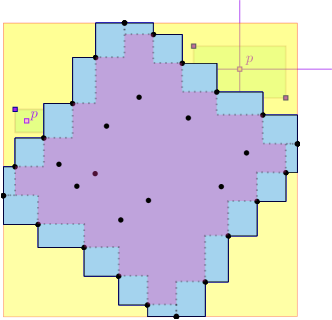
Figure 5.5: The box hull of $P$ Is defined by the four chains/anti-chains that constitute $\mathsf{max}_{\nearrow}\left({P}\right),\mathsf{min}_{\nearrow}\left({P}\right),\mathsf{max}_{\hskip 0.6pt\nwarrow}\left({P}\right),$ and $\mathsf{min}_{\hskip 0.6pt\nwarrow}\left({P}\right)$. Left: If a point $p$ of the union is outside of this perimeter a point of $P$ must exist outside it as well, violating one of the chains. Right: A point set, its rectilinear convex hull (dotted line) and its box hull (full line).

1. Box hull. We fully characterize the union of rectangles associated with RIG, and give simple algorithms to compute it, find a set of $O(n)$ interior disjoint rectangles that partition it, and, given a point in the union, find a rectangle that contains it. We refer to this region induced by the set of points $P$ as the box hull of $P$, see Figure 1.1 and Figure 5.5. See Section 5 for details.

   The box hull is a superset of the rectilinear convex-hull of a point set, and has the advantage of being connected and $x$ and $y$ monotone. To the best of our knowledge this concept was not studied before, and it seems to be natural and more convenient than previous similar concepts.

2. Implicit computation of the RIG. We show that the graph $\mathcal{G}=\mathcal{G}^{\vbox{\hbox{\scalebox{1.0}[0.5]{$\square$}}}}\left({P}\right)$ has a representation as the (edge) disjoint union of $O(n)$ bicliques, where the total weight of the bicliques is $O(n\log^{2}n)$ (and it can be computed at this time). As a reminder, the biclique $L\otimes{R}$ defined by disjoint sets $L,{R}$, is the complete bipartite graph having $L\cup{R}$ as its set of vertices, and edges are only between the two parts. The weight of such a biclique is $\left|{L}\right|+\left|{{R}}\right|$. This implies that while $\mathcal{G}$ might have quadratic number of edges, it still has a compact representation of near linear size.

   To put this result in prospective, it is relatively not hard to observe that such a decomposition can exist by using orthogonal range-searching data-structures. This however seems to lead to bounds of overall size $O(n\log^{3}n)$. Getting rid of the extra logarithmic factor in total weight requires taking a more elaborate approach which is significantly more involved. Similarly, reducing the number of bicliques to linear requires some additional ideas. We consider this to be the main contribution of our work, and it is described in Section 3.

3. Lower bound on the weight of the implicit representation. We prove a lower bound of $\Omega(n\log n)$ on the weight of the biclique cover of an RIG. Thus, our construction above seems to be optimal (up to potentially a single logarithmic factor). See Section 3.5 for details.

4. Depth approximation. Using the small biclique cover we show, for the set of rectangles associated with an RIG, a construction of a data structure for $(1+\varepsilon)$-approximate-depth queries, whose preprocessing phase can be used as a deepest-point $(1+\varepsilon)$-approximation algorithm. While the underlying set of rectangles might have quadratic size, the preprocessing and space used by our data-structure are near linear. Furthermore, queries can be answered in logarithmic time. Interestingly, to this end we replace every biclique by a set of weighted rectangles whose weight approximates the weight induced by the rectangles of the biclique. By approximating “levels” in the bicliques, and using exponential scales and the structure of the bicliques, we are able to do this in near linear time and space, critically using the implicit low-weight biclique representation of the RIG.

A few additional minor new results:

1. In Appendix B.1 we give a tight bound of $\Theta(n\log n)$ on the number of edges in the RIG, with high probability, for a set of $n$ points picked uniformly at random. A concentration result was already shown by Chen et al. [CPST09], but our bound holds with high probability.

2. In Appendix B.2 we prove that the complexity of RIGs is solely due to bicliques. We do so by proving various structural results on RIG. For example, a presence of a biclique with both sides having size at least $k$ implies the existence of three “parallel” long chains that together form this biclique. Similarly, the RIG can not have large (regular) cliques as subgraphs, and any three-sided clique must have a side that contains only a single vertex.

Sketch of computation of the biclique cover of the RIG

Using multi-level orthogonal range searching one can compute for each point $p\in P$ the set of points that it dominates, where the set is represented implicitly as nodes of the data-structure, and every node is associated with all the points stored in its subtree. For our purposes, we need the maxima of each such set, and we need to stitch these together to form a single maxima chain (which is the set of all points that support an empty rectangle with $p$ appearing as the top right corner). Note that a similar procedure is required for the anti-domination relation. To this end, one can compute for each canonical set in the data-structure its maxima, and perform the stitching quickly, see Section 3.2. This yields a representation of all such points that are neighbors of $p$ in the RIG over $P$ using $O(\log^{3}n)$ sets and readily leads to a biclique representation of the RIG of weight $O(n\log^{3}n)$.

To improve this we need to “open” the orthogonal range-searching data-structure. We thus consider the variant where the point $p$ has a higher $y$-coordinate than all the points of $P$ (we refer to $P$ as being a $y$-set in such a case). This turns out to be a more “one-dimensional” problem. We present a stack data-structure that enables us to store and preprocess such queries, where instead of $O(\log^{2}n)$ canonical sets in the output we are able to reduce this number to $O(\log n)$, thus getting the desired improvement. The one dimensional data-structure requires a non-trivial modification of the Bently-Saxe technique coupled with persistence, see Section 3.3.

The number of bicliques this generates is still $O(n\log^{2}n)$. To reduce the number of bicliques further, being somewhat imprecise, we modify the above stack data-structure so that it only generates either “singleton” bicliques or bicliques that have $\Omega(\log n)$ elements on each side (i.e., “heavy bicliques”). The singleton bicliques get merged into star bicliques which results in only $O(n)$ bicliques.

2 Preliminaries

Definition 2.1.

For two points $p,q\in\mathbb{R}^{2}$, let $\mathsf{R}={\vbox{\hbox{\scalebox{1.0}[0.5]{$\square$}}}\left({p,q}\right)}$ denote the minimal axis-parallel closed rectangle that contains $p$ and $q$. Note that $p$ and $q$ form antipodal corners of $\mathsf{R}$. The points $p$ and $q$ support ${\vbox{\hbox{\scalebox{1.0}[0.5]{$\square$}}}\left({p,q}\right)}$, and ${\vbox{\hbox{\scalebox{1.0}[0.5]{$\square$}}}\left({p,q}\right)}$ is the rectangle of influence of $p$ and $q$.

Definition 2.2.

For a set $P$ of $n$ points in $\mathbb{R}^{2}$. The rectangle influence graph (RIG) of $P$ is the graph $\mathcal{G}^{\vbox{\hbox{\scalebox{1.0}[0.5]{$\square$}}}}\left({P}\right)=(P,E)$ where $pq\in E$ $\iff{\vbox{\hbox{\scalebox{1.0}[0.5]{$\square$}}}\left({p,q}\right)}$ does not contain any point of $P$ in its interior. $\mathcal{G}^{\vbox{\hbox{\scalebox{1.0}[0.5]{$\square$}}}}\left({P}\right)$ is also known as the Delaunay graph of $P$ with respect to axis parallel rectangles [CPST09], or negative witness rectangle graph [ADH14]. Similarly, the $\textsf{RIG}_{\!\leq k}$ graph of $P$ is $\mathcal{G}^{\vbox{\hbox{\scalebox{1.0}[0.5]{$\square$}}}}_{\leq k}\left({P}\right)$ = $(P,E_{\leq k})$, where $pq\in E_{\leq k}$ $\iff{\vbox{\hbox{\scalebox{1.0}[0.5]{$\square$}}}\left({p,q}\right)}$ contains at most $k$ points of $P$ in its interior.

Definition 2.3.

A point $p$ dominates (resp. anti-dominates) a point $q$, denoted by $q{\nearrow}p$ (resp. $p{\hskip 0.6pt\nwarrow}q$), if $x(q)<x(p)$ and $y(q)<y(p)$ (resp. $x(p)<x(q)$ and $y(p)>y(q)$).

A ${\nearrow}$-chain is a sequence of points $p_{1},\ldots,p_{k}\in P$, such that $p_{1}{\nearrow}p_{2}{\nearrow}\cdots{\nearrow}p_{k}$. Here, an ${\nearrow}$-antichain corresponds to an ${\hskip 0.6pt\nwarrow}$-chain.

Definition 2.4.

The ${\hskip 0.6pt\searrow}$-chain made of ${\nearrow}$-maximal elements in $P$ is the ${\nearrow}$-maxima of $P$, denoted by $\mathsf{max}_{\nearrow}\left({P}\right)$, which is a sequence of points ordered from left to right. The concept $\mathsf{max}_{\hskip 0.6pt\nwarrow}\left({P}\right)$ is defined in a similar fashion. See Figure 2.1.

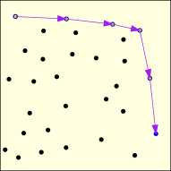
$P$	$\mathsf{max}_{\nearrow}\left({P}\right)$	$\mathsf{max}_{\hskip 0.6pt\nwarrow}\left({P}\right)$

Figure 2.1: The ${\nearrow}$-maxima and ${\hskip 0.6pt\nwarrow}$-maxima of a point set.

The graph whose edge set is formed only by rectangles supported by a pair of points where one dominates (resp. anti-dominates) the other are denoted by $\mathcal{G}^{\vbox{\hbox{\scalebox{1.0}[0.5]{$\square$}}}}_{\nearrow}\left({P}\right)$ (resp. $\mathcal{G}^{\vbox{\hbox{\scalebox{1.0}[0.5]{$\square$}}}}_{\hskip 0.6pt\nwarrow}\left({P}\right)$). These two graphs are edge disjoint and $\mathcal{G}^{\vbox{\hbox{\scalebox{1.0}[0.5]{$\square$}}}}\left({P}\right)=\mathcal{G}^{\vbox{\hbox{\scalebox{1.0}[0.5]{$\square$}}}}_{\nearrow}\left({P}\right)\cup\mathcal{G}^{\vbox{\hbox{\scalebox{1.0}[0.5]{$\square$}}}}_{\hskip 0.6pt\nwarrow}\left({P}\right)$.

3 Biclique cover of $\mathcal{G}^{\vbox{\hbox{\scalebox{1.0}[0.5]{$\square$}}}}\left({P}\right)$

3.1 Definitions

A biclique over (disjoint) sets $X$ and $Y$ is the complete bipartite graph $X\otimes Y=\bigl{(}X\cup Y,\left\{xy\;\middle|\;x\in X,y\in Y\right\}\bigr{)}.$

Definition 3.1.

For a graph $G=(V,E)$, a sequence $\mathcal{C}$ of pairs of sets $\{{R}_{1},{B}_{1}\},\ldots,\{{R}_{t},{B}_{t}\}$ is a biclique cover of $G$ if, for all $i<j$, we have

1. ${R}_{i},{B}_{i}\subseteq V$,

2. ${R}_{i}\cap{B}_{i}=\emptyset$,

3. $E\left({{R}_{i}\otimes{B}_{i}}\right)\cap E\left({{R}_{j}\otimes{B}_{j}}\right)=\emptyset$, and

4. $\cup_{k}({R}_{k}\otimes{B}_{k})=G$.

Thus, for every edge $rb\in E\left({G}\right)$ there exists a unique index $i\in\left\llbracket t\right\rrbracket$ such that $r\in{R}_{i},b\in{B}_{i}$.

The weight of $\mathcal{C}$ is $\omega\left({\mathcal{C}}\right)=\sum_{i=1}^{t}\left({\left|{{R}_{i}}\right|+\left|{{B}_{i}}\right|}\right)$.

The weight of a biclique cover is the space required to store the graph (implicitly) as a list of bicliques, where each biclique is specified by listing its vertices.

Example 3.2.

Note, that any graph $G=(V,E)$ with $n$ vertices $V=\{v_{1},\ldots,v_{n}\}$, has a biclique cover with $n-1$ cliques, with the $i$th biclique having $\{v_{i}\}$ as one side, and all its neighbors in $V^{i+1}=\{v_{i+1},\ldots,v_{n}\}$ on the other side. Formally, $G=\cup_{i}\bigl{(}\{v_{i}\}\otimes(V^{i+1}\cap\Gamma\left({v_{i}}\right))\bigr{)}$, where $\Gamma\left({v}\right)$ denotes the set of neighbors of $v$ in $G$. Of course, the weight of this cover is (asymptotically) the number of edges in the graph, thus the challenge is to compute a cover of a graph with a near-linear number of bicliques and small total weight. A random graph where each edge is chosen with probability half readily shows that there are graphs where the weight is at least quadratic in any biclique cover. Namely, graphs in general do not have near-linear weight biclique cover.

3.2 Stitching maximas quickly

Consider a (balanced) binary search tree $T$ that stores a sequence $S=\left({s_{1}\prec s_{2}\prec\cdots\prec s_{n}}\right)$ in its leaves according to some linear order $\prec$. For a node $v\in T$, let $L(v)$ denote the sorted list of elements stored in its subtree.

Observation 3.3.

For any two elements $s_{i},s_{j}\in S$, with $i<j$, there are $t\leq 2\cdot\mathrm{height}(T)-1$ nodes $v_{1},\ldots v_{t}$ of $T$, such that $s_{i},\ldots s_{j}=L(v_{1})\cup\cdots\cup L(v_{t})$. The sequence $v_{1},\ldots,v_{t}$ is the implicit representation of the (explicit) sequence $s_{i},\ldots,s_{j}$. The nodes $v_{1},\ldots,v_{t}$ appear on or adjacent to the two paths in the tree from the root to $s_{i}$ and $s_{j}$, so computing this representation takes $O(\mathrm{height}\left({T}\right))$ time.

Lemma 3.4.

Let ${\mathsf{r}}_{1}$ and ${\mathsf{r}}_{2}$ be two disjoint rectangles with their respective maximas $L_{1}=\mathsf{max}_{\nearrow}\left({{\mathsf{r}}_{1}\cap P}\right)$ and $L_{2}=\mathsf{max}_{\nearrow}\left({{\mathsf{r}}_{2}\cap P}\right)$ stored in balanced binary search trees $T_{1}$ and $T_{2}$ respectively (say, the points are stored sorted in increasing $x$-axis order). Then, one can compute, in $O(\log n)$ time, $m=O(\log n)$ nodes $v_{1},\ldots,v_{m}$, such that $L(v_{1})|\cdots|L(v_{m})$ is $L=\mathsf{max}_{\nearrow}\left({({\mathsf{r}}_{1}\cup{\mathsf{r}}_{2})\cap P}\right)$, where $|$ denotes concatenation and $n=\left|{P}\right|$. Specifically, if $L_{1}$ and $L_{2}$ are represented by lists of nodes of size $\leq t$, then $L$ can be computed in $O(t+\log n)$ time.

Proof:

The algorithm checks if ${\mathsf{r}}_{1}$ and ${\mathsf{r}}_{2}$ are separated by a horizontal line, a vertical line, or both. The various cases are handled in similar fashion, so we describe only the case that ${\mathsf{r}}_{1}$ and ${\mathsf{r}}_{2}$ are horizontally separated, and ${\mathsf{r}}_{1}$ is vertically above ${\mathsf{r}}_{2}$, see Figure 3.1.

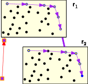
Figure 3.1:

Let $L_{i}=\mathsf{max}_{\nearrow}\left({{\mathsf{r}}_{i}\cap P}\right)$ for $i\in\{1,2\}$. Let $x$ be the $x$-coordinate of the last point of $L_{1}$, and observe that the merged maxima is the result of throwing away all the points of $L_{2}$ that have smaller $x$-coordinate than $x$ from $L_{2}$ and concatenating the two sequences. Namely, the merged maxima is $L_{1}\cup(L_{2}\cap(x,\infty))$, where $L_{2}\cap(x,\infty)$ denotes the desired suffix of $L_{2}$. By Observation 3.3 this suffix has the desired representation as a sequence of $O(\log n)$ nodes. Prefixing this sequence by the root of the tree representing $L_{1}$ yields the desired result.

The second claim follows by observing that computing a subsequence stored in a node $v$, between two given elements, can be done in $O(\log n)$ time, if implicit representation is sufficient. It is easy to verify that the split and concatenation operations required by the above, can be implemented by computing a subsequence, see Observation 3.3, which might yield an implicit representation of size $O(t+\log n)$, and then concatenating this nodes list with the list of nodes representing the other set. In either case, this can be done in $O(t+\log n)$ time.  

3.3 A helper data-structure: Stack with range queries

In the following, we describe a stack data-structure that stores a sequence of elements (e.g. points) with an associated real value (e.g. the points’ $x$ coordinates). Note that the elements must be inserted in increasing order. The following operations are supported:

1. ${{\color[rgb]{0.59,0,0.66}\texttt{\bf{push}}}}(x)$: Push $x$ to the stack.

2. ${{\color[rgb]{0.59,0,0.66}\texttt{\bf{pop}}}}(k$): Pops the top $k$ elements from the stack.

3. ${{\color[rgb]{0.59,0,0.66}\texttt{\bf{report}}}}(x,y)$: Output a representation of the subsequence of the elements stored in the stack between $x$ and $y$.

In addition, the data-structure can declare that a specific list/set of elements is canonical. For a list of size $t$, making it canonical costs $O(t)$ time. Importantly, the above report output is a list of canonical sets.

Implementation

We follow the Bently and Saxe [BS80] technique. The basic building block would be a perfect binary tree. Such a tree $T$ storing $2^{t}$ elements has rank $t$ (i.e., height), where all the values are stored in the leafs of $T$. Let $L\left({T}\right)$ denote the list/sequence of elements stored in $T$.

At any given point in time the stack contains a list of $O(\log n)$ such trees $T_{1},...,T_{m}$, referred to as the current forest, with $L\left({T_{1}}\right)|\ldots|L\left({T_{m}}\right)$ being the content of the stack (i.e., the top of the stack is the last element). The following invariants are maintained:

1. $|T_{i}|\geq|T_{i+1}|$, for all $i$.

2. There are at most two trees with the same rank in this list.

The specific operations are implemented as follows:

1. ${{\color[rgb]{0.59,0,0.66}\texttt{\bf{push}}}}(x)$: A tree of rank zero containing this element and appending it to the end of the list of trees in the stack. Now, if the last three trees in the stack have the same rank, say $t$, the first two trees are merged into a new tree of rank $t+1$, and the new tree replaces the old two trees. This is repeated till no three trees in the list of the stack are of the same rank (i.e., the above invariants are maintained). Whenever a new tree is being created it is being canonized (i.e. registered as a canonical set). This is implemented in a mundane way during merge – the new tree is formed by (deep) copying its two subtrees, and by creating a new root node.

2. ${{\color[rgb]{0.59,0,0.66}\texttt{\bf{pop}}}}(k)$: The data-structure locates the tree $T_{i}$ in the forest containing the $k$th value from the end of the stack. It then removes the following trees $T_{j}$, with $j>i$ from the forest. Let $r=\mathrm{rank}\left({T}\right)$. The data-structure breaks $T_{i}$ into $u<r$ trees $T_{1}^{\prime},\ldots,T_{u}^{\prime}$, such that $L\left({T_{1}^{\prime}}\right)|\cdots|L\left({T_{1}u^{\prime}}\right)$ are all the elements appearing before $x$ in $T_{i}$. The data-structure replaces $T_{i}$ in the forest by $T_{1}^{\prime},\ldots,T_{u}^{\prime}$. Note, that as $\mathrm{rank}\left({T_{1}^{\prime}}\right)>\cdots>\mathrm{rank}\left({T_{u}^{\prime}}\right)$, this preserves the invariants specified above. Furthermore, $T_{1}^{\prime},\ldots,T_{u}^{\prime}$ are trees that were created earlier by the data-structure, so ${{\color[rgb]{0.59,0,0.66}\texttt{\bf{pop}}}}(k)$ is implemented in $O(\log n)$ time.

3. ${{\color[rgb]{0.59,0,0.66}\texttt{\bf{report}}}}(x,y)$: Scanning the forest, the algorithm computes the range of trees $T_{\alpha},\ldots,T_{\beta}$ that their lists contain the desired elements. Using binary search on $T_{\alpha}$ and $T_{\beta}$, the algorithm computes $O(\log n)$ nodes (an internal node of tree can be treated as its own tree) that lists the elements that are in the desired range. Let $\mathcal{F}_{\alpha}$ and $\mathcal{F}_{\beta}$ be these forests computed for $T_{\alpha}$ and $T_{\beta}$ respectively. Clearly, the desired output is $\mathcal{F}_{\alpha}|T_{\alpha+1}|\cdots|T_{\beta-1}|\mathcal{F}_{\beta}$, a list of $O(\log n)$ trees, and it can be computed in $O(\log n)$ time.

3.3.1 Performance

Lemma 3.5.

The above data structure performs a sequence of $n$ push/pop operations in $O(n\log n)$ time, and this also bounds the total size of the canonical sets. The total number of canonical sets is $O(n)$. A reporting query takes $O(\log n)$ time, and returns $O(\log n)$ canonical sets per query.

Proof:

In order to bound the total size of the trees created by $n$ operations, consider the set of trees of rank $k$ created during the lifetime of the data structure. Let $o_{1},...,o_{n}$ be the sequence of operations performed. The operation $o_{t}$ is the step at time $t$. A tree $T$ of rank $k$ was created at time $t$ if $o_{t}$ is the push operation that resulted in the creation of $T$ by merging two trees of rank $k-1$.

We claim that the time difference between the creation of two trees $T,T^{\prime}$, both of rank $k$, at times, say, $t$ and $t^{\prime}$ respectively where $t<t^{\prime}$. is $\geq 2^{k-1}-1$. At time $t-1$, i.e. just before $o_{t}$ was executed, the current forest had two trees of rank $k-1$, after the push operation $o_{t}$, a cascade of merges of trees resulted in the creation of $T$. Note that a merge of two trees of rank $u$ is triggered if the forest has three trees of rank $u$. After the merge, there is exactly one tree in the forest of rank $u$. Namely, immediately after $o_{t}$ was executed, the forest has exactly one tree of rank $u$ for $u=0,\ldots,k-1$.

If the sets of values stored in $T$ and $T^{\prime}$ are disjoint, it is clear that at least $2^{k}/2$ more insertions are required in order for another tree of size $2^{k}$ to be created even if no pop operations were executed between times $t$ and $t^{\prime}$. If the sets of values stored in $T$ and $T^{\prime}$ are not disjoint, then consider the first time $t^{\prime\prime}$, $t<t^{\prime\prime}<t^{\prime}$, in which a value stored in $T$ is popped alongside all elements inserted after it. This “shatters” the tree $T$ in the forest, replacing it by a sequence of subtrees. Importantly, all these subtrees have each unique rank, and there are no other trees in the forest with this rank (at this time). Specifically, after $o_{t^{\prime\prime}}$ the forest has at most one tree of rank $k-1$, and the same holds for smaller ranks. In particular, the total size of the elements stored in these “tail” trees is at most $\gamma=2^{k}-1$. Thus, at least $3\cdot 2^{k-1}-\gamma=2^{k-1}-1$ more elements have to be pushed into the stack before the forest would contain three blocks of rank $k-1$ and trigger the merge creating $T$, as claimed.

Thus, the number of trees of rank $k$ created during the course of $n$ operations, is $O(n/2^{k})$, and the overall size of all the canonical sets is at most $\sum_{k=1}^{\log n}2^{k}O(n/2^{k})=O(n\log n)$.  

Remark 3.6 (Persistence).

A minor technicality is that we need to perform the ${{\color[rgb]{0.59,0,0.66}\texttt{\bf{report}}}}(x,y)$ query on the stack at the point in time just before a value larger than $y$ was inserted. To this end, after each operation the data-structure creates a copy of the forest – as the forest is simply a list of $O(\log n)$ trees, this can be done in $O(\log n)$ time. Now, given a query ${{\color[rgb]{0.59,0,0.66}\texttt{\bf{report}}}}(x,y)$, the algorithm first does a binary search to find the copy of the forest at the “right” time, and then performs the query on this version. A more efficient persistence scheme might be possible here, but it is irrelevant for our purposes.

3.4 Extracting the maxima

Lemma 3.7.

Let $P$ be a set of $n$ points in the plane in general position. The graph $\mathcal{G}^{\vbox{\hbox{\scalebox{1.0}[0.5]{$\square$}}}}\left({P}\right)$ has a biclique cover with $O(n\log n)$ bicliques, and total weight $O(n\log^{2}n)$. The biclique cover can be computed in $O(n\log^{2}n)$ time.

Proof:

We describe the construction for $\mathcal{G}^{\vbox{\hbox{\scalebox{1.0}[0.5]{$\square$}}}}_{\nearrow}\left({P}\right)$. A similar construction applies to $\mathcal{G}^{\vbox{\hbox{\scalebox{1.0}[0.5]{$\square$}}}}_{\hskip 0.6pt\nwarrow}\left({P}\right)$, and together they form the desired cover. Let $Y=Y(P)$ be the set of $y$-coordinates of the points of $P$. Let $T_{Y}$ be a balanced binary search tree on the points of $Y$. A $y$-set is the set of (original) points of $P$ stored in a subtree of $T_{Y}$. Given an unbounded downward ray $\rho$ on the $y$-axis, the set $\rho\cap Y$ can be represented as the disjoint union of $\left\lceil{\log_{2}n}\right\rceil$ $y$-sets.

Consider such a $y$-set, and its corresponding subset $Z\subseteq P$. Assume the points of $Z$ are (pre)sorted by the $x$-axis, and $Z=\{p_{1},\ldots,p_{u}\}$. The algorithm inserts the points of $Z$ in this order into the stack data structure described in Lemma 3.5 while maintaining $\mathsf{max}_{\nearrow}\left({p_{1},\ldots,p_{i}}\right)$. Namely, before $p_{i}$ is pushed, the algorithm pops from the top of the stack all the points that $p_{i}$ dominates. The algorithm performs this construction on all the $y$-sets of $T_{Y}$. The total size of the $y$-sets is $O(n\log n)$. Presorting the points of $P$ by the $x$ and $y$-axis, and computing these data-structures in a top-down recursive fashion on $T_{Y}$ can be done in $O(n\log^{2}n)$ time overall. The total number of the canonical sets created in all the stacks is $O(n\log n)$.

Now, for each point $p\in P$ the algorithm computes the maxima of the points it dominates. Indeed, for a point $p$, the algorithm computes the $O(\log n)$ disjoint $y$-sets whose union is all the points of $P$ with $y$ coordinate smaller than $p$. For each such $y$-set the algorithm precomputed the data-structure of Lemma 3.5, and it can extract the maxima in the $y$-set up to the point $p$. Using the stitching algorithm of Lemma 3.4 one can find the maxima of the points that $p$ dominates. This maxima would be represented by the disjoint union of $O(\log^{2}n)$ canonical sets.

In detail, given a point $p=(x,y)\in P$ we compute a disjoint union of $m=O(\log n)$ $y$-sets $Y_{1},\ldots,Y_{m}$ such that $\cup_{i}Y_{i}$ is the set of all points with $y$-coordinate smaller than $p$. Assume that all the points of $Y_{i}$ have bigger $y$ coordinates than the points of $Y_{i+1}$, for all $i$. Let $\mathcal{Q}=(-\infty,x)\times(-\infty,y)$. Clearly, all the Delaunay rectangles having $p$ on the right-top corner have a point of $\mathsf{max}_{\nearrow}\left({\mathcal{Q}\cap P}\right)$ on the other corner, and also $\mathcal{Q}\cap P=\cup_{i}(\mathcal{Q}\cap Y_{i})$. Let $L_{1}^{\prime}=\mathsf{max}_{\nearrow}\left({\mathcal{Q}\cap Y_{1}}\right)$ – this can be computed in $O(\log n)$ time using the stack data-structure computed for $Y_{1}$, and let $r_{1}$ be the $x$-coordinate of the last point of $L_{1}$. Naively, one can repeat this process for all $i$, computing $L_{i}^{\prime}=\mathsf{max}_{\nearrow}\left({\mathcal{Q}\cap Y_{i}}\right)$. The desired maxima is the “stitched” maxima of these maximas. It is more efficient to do this stitching process directly. Indeed, let $L_{i}=\mathsf{max}_{\nearrow}\left({\cup_{k=1}^{i}L_{k}^{\prime}}\right)$, with $L_{1}=L_{1}^{\prime}$. Let $r_{i}$ be the $x$-coordinate of the rightmost point in $L_{i}$. The algorithm now adds the next portion of the maxima that uses points of $Y_{i+1}$. To this end, using persistence, the data-structure recovers the last time, say $t_{i+1}$, when a point of $Y_{i+1}\cap\mathcal{Q}$ was inserted into its stack. Let $S_{i+1}$ denote this snapshot of this stack at time $t_{i+1}$. The algorithm then extracts the maxima of $Y_{i+1}$ appearing in $L_{i+1}$ by performing the query ${{\color[rgb]{0.59,0,0.66}\texttt{\bf{report}}}}(r_{i},x)$. The algorithm repeats this process for the next value of $i$ till the whole maxima is extracted. This takes $O(\log^{2}n)$ time and results in a representation of $\mathsf{max}_{\nearrow}\left({\mathcal{Q}\cap P}\right)$ using $O(\log^{2}n)$ canonical sets. We register $p$ with all of these canonical sets.

At the end of this process, every canonical set $X$ has a set of points $Y$ registered with it. The algorithm outputs $X\otimes Y$ as one of the computed bicliques. The bound on the size of the bicliques is immediate – the total size of the canonical sets is $O(n\log^{2}n)$, and each point of $P$ is registered with $O(\log^{2}n)$ canonical sets. As for their total number, Lemma 3.5 implies that the number of canonical sets every $y$-set induces is proportional to its cardinality. Thus, the overall number of canonical sets is $O(n\log n)$. Every canonical set $X$ has a set of $Y$ of (query) points registered with it, and give rise to the biclique $X\otimes Y$. Thus, the total number of bicliques is $O(n\log n)$.  

Being a bit more careful, one can reduce the number of bicliques to linear while keeping the total weight (asymptotically) the same.

Theorem 3.8.

Let $P$ be a set of $n$ points in the plane in general position. The graph $\mathcal{G}^{\vbox{\hbox{\scalebox{1.0}[0.5]{$\square$}}}}\left({P}\right)$ has a biclique cover with $O(n)$ bicliques, and total weight $O(n\log^{2}n)$. The biclique cover can be computed in $O(n\log^{2}n)$ time.

Proof:

The idea is two folds. The basic idea is that bicliques involving a singleton on one side are fine – there are going to be only $n$ such bicliques globally. Similarly, one can argue that the number of large bicliques involving a large canonical set (roughly of size $\Omega(\log^{2}n)$) on one side is globally bounded by $O(n)$.

The problem is thus with middling size canonical sets of size roughly $O(\log n)$. We first describe how to reduce the number of canonical sets used by the stack data-structure. The idea is to add a buffer of size (say) $\tau=3\left\lceil{\log n}\right\rceil$ of singletons that will be stored as they are. Whenever the buffer is filled the algorithm extracts the last $\left\lceil{\log n}\right\rceil$ elements, and create a canonical set for these elements, deleting these sets from the buffer (which is a FIFO queue). It is easy to verify that the previous stack construction can be easily modified to work with this buffer thus creating canonical sets only of size $\geq\tau$. The number of non-singleton canonical sets created by the stack is therefore

$$\sum_{k=\left\lfloor{\log\tau}\right\rfloor}n/2^{k}=O(n/\tau)=O(n/\log n).$$

We apply the same idea to the $y$-strips. We only build the stack data-structure for strips that contain more than $\tau$ points. Formally, we partition the point sets into strips of size $\tau$ in the $y$-order, and build balanced binary tree on these strips. Now, a query would involve $O(\log n)$ $y$-sets (each of size at least $\tau$) where potentially the smallest strip might contain $\tau$ points, and the query quadrant intersects it only partially. The query in this top strip is answered directly by scanning (i.e., we compute the maxima of the points in this strip inside the query quadrant and register the query point with each point on the maxima), while for any other of the $y$-strips we use the stitching algorithm described in Lemma 3.7. Clearly, as before, there are $O(\log n)$ $y$-strips involved with the query and each one returns $O(\log n)$ canonical sets, thus reproducing the old bound on the total weight of the bicliques.

As for the overall number of bicliques, observe that every biclique rises out of a canonical set in one of the (modified) stack data-structures. If a $y$-set has $t$ points then the total number of canonical sets it defines is $O(t/\log n)$ (ignoring singletons, since these ones are already counted directly). Thus, since the total number of $y$-strips of size $2^{i}\tau$ is $n/(2^{i}\tau)$ and each one of them contributes $O(2^{i}\tau/\log n)=O(2^{i})$ (non-singleton) canonical sets, we conclude that the total number of (non-singleton) canonical sets over all $y$ strips is

$$O\Bigl{(}\sum\nolimits_{i=0}^{O(\log n)}\frac{n}{2^{i}\tau}\cdot 2^{i}\Bigr{)}=O(n).$$

 

Observation 3.9.

Let $P$ be a set of points in the plane, and let $\mathcal{R}=\mathcal{R}^{\vbox{\hbox{\scalebox{1.0}[0.5]{$\square$}}}}\left({P}\right)$, and let $\mathcal{C}$ be the biclique cover computed by Theorem 3.8. Each biclique corresponds to two disjoint point sets $P_{i},Q_{i}\subseteq P$, such that $\mathcal{R}=\cup_{i}{\vbox{\hbox{\scalebox{1.0}[0.5]{$\square$}}}\left({P_{i},Q_{i}}\right)}$, where ${\vbox{\hbox{\scalebox{1.0}[0.5]{$\square$}}}\left({P_{i},Q_{i}}\right)}=\cup_{p\in P_{i},q\in Q_{i}}\{{\vbox{\hbox{\scalebox{1.0}[0.5]{$\square$}}}\left({p,q}\right)}\}$. Furthermore $P_{i}$ and $Q_{i}$ are separable by both a horizontal and vertical lines. Finally, we can assume that each of the sets $P_{i},Q_{i}$ are available as a sequence sorted by both $x$-axis and $y$-axis order. This provides us with an implicit efficient representation of $\mathcal{R}$ that can be computed in $O(n\log^{2}n)$ time, made out of $O(n)$ pairs, and of total weight $O(n\log^{2}n)$.

Corollary 3.10.

The graph $\mathcal{G}^{\vbox{\hbox{\scalebox{1.0}[0.5]{$\square$}}}}_{\leq k}\left({P}\right)$ has a biclique cover of size $O(kn)$. Furthermore, the total weight of the cover is $O(kn\log^{2}n)$, and it can be computed in $O(kn\log^{2}n)$ time.

Proof:

By creating $k$ stack data structures for every canonical slab we can easily maintain the first $k$ levels of, say ${\nearrow}$-maxima, each contained in a separate stack. An introduction of a new point $p$ becomes a $k$-step process starting with the insertion of the point to the upper-most stack maintaining the maxima chain, but now instead or simply deleting the chain prefix that is now in the second level of maxima, that sequence of points is now inserted simultaneously to the next stack. This is possible since $p$, being inserted as the rightmost point seen so far, dominates a continuous prefix of every level of the $k$ ${\nearrow}$-maximas, and thus we can, for every level, report and remove the points dominated by $p$ using the operations as they are described in Section 3.3, and insert the points from the previous level by using an individual insert operation for every point. Notice that every point $q_{i+1}$ that remains in the $(i+1)$th level after the deletion step is to the left of any point $q_{i}$ inserted (i.e. deleted from the $i$th level) since otherwise we get that $q_{i}{\nearrow}q_{i+1}$ which is a contradiction. Since every point is inserted and deleted exactly once at any level the size and time complexity are $O(kn\log^{2}n)$ as stated.  

3.5 A lower bound

Theorem 3.11.

[BS07] The weight of any biclique cover of $K_{n}$ is $\Omega(n\log n)$, where $K_{n}$ denotes the complete graph over $n$ vertics.

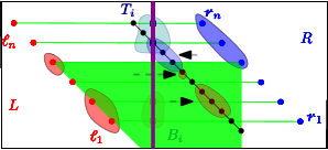
Figure 3.2: Illustration of the construction in Lemma 3.12. Left: the set of $2n$ points ${R}$ and ${B}$ and a biclique $\{A_{i},B_{i}\}$. Right: An illustration of the construction of $\{A^{\prime}_{i},B^{\prime}_{i}\}$ as a projection to a 1-dimensional space

Lemma 3.12.

There exists a set $P$ of $n$ points, such that any biclique cover of $\mathcal{G}^{\vbox{\hbox{\scalebox{1.0}[0.5]{$\square$}}}}\left({P}\right)$ has weight $\Omega(n\log n)$.

Proof:

Let $L$ and ${R}$ be two sets of points, defined by

$$L=\left\{\mathcalb{l}_{i}=(-i,i)\;\middle|\;i\in\left\llbracket n\right\rrbracket\right\}\qquad\text{and}\qquad{R}=\left\{\mathcalb{r}_{i}=(2n-i,i)\;\middle|\;i\in\left\llbracket n\right\rrbracket\right\}.$$

See Figure 3.2. Let $P=L\cup{R}$, $\mathcal{G}=\mathcal{G}^{\vbox{\hbox{\scalebox{1.0}[0.5]{$\square$}}}}\left({P}\right)$, and $\mathcal{C}$ be any biclique cover of $\mathcal{G}$. Next, consider the restriction of the biclique cover to the two sides (some edges would no longer be covered):

$$\mathcal{D}=\left\{(X\cap L)\otimes(Y\cap{R}),(X\cap{R})\otimes(Y\cap L)\;\middle|\;X\otimes Y\in\mathcal{C}\right\}.$$

Observe that $\omega\left({\mathcal{C}}\right)=\Theta(\omega\left({\mathcal{D}}\right))$. We rewrite $\mathcal{D}=\{L_{1}\otimes{R}_{1},\ldots,L_{s}\otimes{R}_{s}\}$, where $L_{i}\subset L$, and ${R}_{i}\subset{R}$, for all $i$. For all pairs $L_{i}\otimes{R}_{i}\in\mathcal{D}$ and all points $\mathcalb{l}_{\lambda}=(-\lambda,\lambda)\in L_{i}$ and $\mathcalb{r}_{\rho}=(2n-\rho,\rho)\in{R}_{i}$, we have that $\lambda\leq\rho$, as otherwise $\lambda>\rho$, and the associated rectangle ${\mathsf{r}}={\vbox{\hbox{\scalebox{1.0}[0.5]{$\square$}}}\left({\mathcalb{l}_{\lambda},\mathcalb{r}_{\rho}}\right)}$ contains the point $\mathcalb{l}_{\lambda-1}=(-\lambda+1,\lambda-1)\in L$, which implies that ${\mathsf{r}}\notin\mathcal{R}^{\vbox{\hbox{\scalebox{1.0}[0.5]{$\square$}}}}\left({P}\right)$. Namely, $\mathcalb{l}_{\lambda}\mathcalb{r}_{\rho}\notin E\left({\mathcal{G}}\right)$ for $\lambda>\rho$.

For a set of points $Z$, let $Y(Z)=\left\{y\;\middle|\;(x,y)\in Z\right\}$ be the set of $y$-coordinates appearing in points of $Z$. Let $B_{i}^{\prime}=Y(L_{i})$, $T_{i}^{\prime}=Y({R}_{i})$, and $M_{i}^{\prime}=B_{i}^{\prime}\cap T_{i}^{\prime}$, for all $i$. Observe that since $\mathcalb{l}_{\lambda}\mathcalb{r}_{\rho}\notin E\left({\mathcal{G}}\right)$ for $\lambda>\rho$, $\left|{M_{i}^{\prime}}\right|\leq 1$. Let $B_{i}=B_{i}^{\prime}\setminus M_{i}^{\prime}$ and $T_{i}=T_{i}^{\prime}\setminus M_{i}^{\prime}$, for all $i$. Consider the biclique cover

$$\mathcal{F}=\left\{B_{i}\otimes T_{i},(B_{i}\cup T_{i})\otimes M_{i}^{\prime}\;\middle|\;i\in\left\llbracket s\right\rrbracket\bigr{.}\right\}.$$

Here, if either side of a biclique is empty (probably $M_{i}^{\prime}$) then it is not included in this cover. Clearly $\omega\left({\mathcal{F}}\right)=\Theta(\omega\left({\mathcal{D}}\right)=\Theta(\omega\left({\mathcal{C}}\right)$. Observe that for any $1\leq i<j\leq n$ there exits a pair $X\otimes Y\in\mathcal{F}$ such that $ij\in E\left({\mathcal{F}}\right)$. Namely, $\mathcal{F}$ is a (disjoint) biclique cover of the clique $\binom{\left\llbracket n\right\rrbracket}{2}$, and by Theorem 3.11 we have $\omega\left({\mathcal{C}}\right)=\Theta(\omega\left({\mathcal{F}}\right))=\Omega(n\log n)$.  

4 Approximating the depth

For a set of regions $\mathcal{O}$ in the plane, the depth of a point $p\in\mathbb{R}^{2}$, is the number of regions in $\mathcal{O}$ that contains $p$. That is $\mathrm{d}_{\mathcal{O}}\left({p}\right)=\left|{\left\{\mathcalb{r}\in\mathcal{O}\;\middle|\;p\in\mathcalb{r}\right\}}\right|$. The maximum depth of $\mathcal{O}$ is $\mathrm{d}_{\max}\left({\mathcal{O}}\right)=\max_{p\in\mathbb{R}^{2}}\mathrm{d}_{\mathcal{O}}\left({p}\right)$. For a point set $P$, consider the set of rectangles they induce $\mathcal{R}=\mathcal{R}^{\vbox{\hbox{\scalebox{1.0}[0.5]{$\square$}}}}\left({P}\right)$, see Eq. (1.1). For a point $p$, let $\mathrm{d}^{\vbox{\hbox{\scalebox{1.0}[0.5]{$\square$}}}}\left({p}\right)=\mathrm{d}_{\mathcal{R}}\left({p}\right)$ denote the rectangular depth of $p$. Similarly, let $\mathrm{d}^{\vbox{\hbox{\scalebox{1.0}[0.5]{$\square$}}}}_{\max}\left({P\bigr{.}}\right)=\mathrm{d}_{\max}\left({\mathcal{R}}\right)$ denote the maximum rectangular depth of $P$.

Lemma 4.1.

Let $P$ be a set of $n$ points in the plane, one can compute, in $O(n\log^{4}n)$ time, a point $p$ such that $\mathrm{d}^{\vbox{\hbox{\scalebox{1.0}[0.5]{$\square$}}}}\left({p}\right)=\Omega(\mathrm{d}^{\vbox{\hbox{\scalebox{1.0}[0.5]{$\square$}}}}_{\max}\left({P\bigr{.}}\right)/\log n)$.

Proof:

We compute the implicit representation ${\vbox{\hbox{\scalebox{1.0}[0.5]{$\square$}}}\left({P_{1},Q_{1}}\right)},\ldots,{\vbox{\hbox{\scalebox{1.0}[0.5]{$\square$}}}\left({P_{s},Q_{s}}\right)}$ of $\mathcal{R}=\mathcal{R}^{\vbox{\hbox{\scalebox{1.0}[0.5]{$\square$}}}}\left({P}\right)$, as described in Observation 3.9. It is now straightforward to verify that for the set of rectangles ${\vbox{\hbox{\scalebox{1.0}[0.5]{$\square$}}}\left({P_{i},Q_{i}}\right)}$, the depth along a horizontal line $\ell$ can be described by a weighted set of $O(\left|{P_{i}}\right|+\left|{Q_{i}}\right|)$ interior disjoint intervals (that can also be computed in this time).

Thus, computing the maximum depth on $\mathcal{R}$ on a vertical line $\ell$ can be reduced to computing the maximum depth of a point in a set of weighted intervals, where the total number of intervals is $\omega\left({\mathcal{C}}\right)=O(n\log^{2}n)$. This in turn can be done in $O(n\log^{3}n)$ time.

We now apply the standard divide-and-conquer approach. Take the vertical line that is the median on the $x$-axis of the points of $P$. Compute the maximum depth point on this line. Now, compute the maximum depth recursively on the point set on the right, and the point set on the left. Return the maximum depth point out of the three candidates computed. Observe that the recursion depth is $h=O(\log n)$, and this decomposes $\mathcal{R}$ into $O(\log n)$ disjoint sets. One of these sets the maximum rectangular depth is $\mathrm{d}^{\vbox{\hbox{\scalebox{1.0}[0.5]{$\square$}}}}_{\max}\left({P\bigr{.}}\right)/h$, which is a lower bound on the depth of the point computed by the algorithm.  

Lemma 4.2.

For any $\varepsilon\in(0,1)$ and a point set $P$ of $n$ points in the plane, one can construct, in $O(\varepsilon^{-2}n\log^{3}n)$ time/space, a data structure that $(1-\varepsilon)$-approximates rectangular depth queries in $\mathcal{R}^{\vbox{\hbox{\scalebox{1.0}[0.5]{$\square$}}}}\left({P}\right)$. Specifically, given a query point $q$, the data-structure returns, in $O(\log n)$ time, a value $\alpha$ such that $(1-\varepsilon)\mathrm{d}^{\vbox{\hbox{\scalebox{1.0}[0.5]{$\square$}}}}\left({q}\right)\leq\alpha\leq\mathrm{d}^{\vbox{\hbox{\scalebox{1.0}[0.5]{$\square$}}}}\left({q}\right)$.

Proof:

First compute the implicit decomposition ${\vbox{\hbox{\scalebox{1.0}[0.5]{$\square$}}}\left({P_{1},Q_{1}}\right)},\ldots,{\vbox{\hbox{\scalebox{1.0}[0.5]{$\square$}}}\left({P_{s},Q_{s}}\right)}$ of $\mathcal{R}=\mathcal{R}^{\vbox{\hbox{\scalebox{1.0}[0.5]{$\square$}}}}\left({P}\right)$, using Theorem 3.8. The idea is to replace each set of rectangles ${\vbox{\hbox{\scalebox{1.0}[0.5]{$\square$}}}\left({P_{i},Q_{i}}\right)}$, which is of size $\left|{P_{i}}\right|\cdot\left|{Q_{i}}\right|$ by a set of interior disjoint weighted rectangles that approximates the depth they provide, and this new set has nearly linear size in $\left|{P_{i}}\right|+\left|{Q_{i}}\right|$.

So, consider such a pair ${\vbox{\hbox{\scalebox{1.0}[0.5]{$\square$}}}\left({U,V}\right)}$. By Observation 3.9 the point sets $U$ and $V$ are quadrant separated, and form each (say) a ${\hskip 0.6pt\nwarrow}$-chain, so assume (without loss of generality) that $V{\nearrow}U$. Let $U=\{u_{1},\ldots,u_{s}\}$ and $V=\{v_{1},\ldots,v_{t}\}$ be the two point sets sorted from left to right, and let $N=\left|{U}\right|+\left|{V}\right|=s+t$. Consider the arrangement $\mathcal{A}=\mathcal{A}\left({{\vbox{\hbox{\scalebox{1.0}[0.5]{$\square$}}}\left({U,V}\right)}\bigr{.}}\right)$.

Let $\mathsf{B}_{k}$ be the boundary of the (closure of the) set of all the points that dominate $k$ or more points of $V$. The set $\mathsf{B}_{k}$ is the $k$th bottom staircase of $\mathcal{A}$. The $k$th top staircase $\mathsf{T}_{k}$ is defined analogously for $U$. If a point $p\in\mathbb{R}^{2}$ is between $\mathsf{B}_{k}$ and $\mathsf{B}_{k+1}$, and between $\mathsf{T}_{\ell}$ and $\mathsf{T}_{\ell+1}$, then $\mathrm{d}_{{\vbox{\hbox{\scalebox{1.0}[0.5]{$\square$}}}\left({U,V}\right)}}\left({p}\right)=k\ell$. See Figure 4.1.

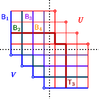
Figure 4.1: The structure of the staircases induced by the quadrant separated ${\nearrow}$-chains $U$ and $V$.

Observe that the vertices of a top chain are quadrant-separated from the vertices of a bottom chain. Furthermore, given two bottom chains $\mathsf{B}_{\alpha}$ and $\mathsf{B}_{\beta}$, with $\alpha<\beta$, one can compute an axis aligned polygonal line $\gamma$ in between them of complexity $O\bigl{(}\left|{V}\right|/(\beta-\alpha)\bigr{)}$. Specifically, $\gamma$ starts between the top endpoints of $\mathsf{B}_{\alpha}$ and $\mathsf{B}_{\beta}$, and ends similarly between the right endpoints of the two staircases. Indeed, start with top vertex of $\mathsf{B}_{\beta}$ and move vertically down till hitting $\mathsf{B}_{\alpha}$. When this happens $\gamma$ changes direction and moves horizontally from left to right till hitting $\mathsf{B}_{\beta}$, then $\gamma$ changes back to moving vertically down. Keeping this alternation till exiting on the right. To see the bound on the complexity of the curve consider the grid formed by horizontal and vertical lines passing through the points of $V$, and observe that the interior of every straight segment of $\gamma$ intersects $\beta-\alpha-1$ of these lines. Since $\gamma$ can intersect such a line only once, and there are $2\left|{V}\right|$ such lines the bound follows.

For $i=1,\ldots,\mu=\left\lceil{6/\varepsilon}\right\rceil$, let $\alpha_{i}=i$. For $i>\mu$, let $\alpha_{i}=\min(\left|{V}\right|,\left\lceil{(1+\varepsilon/3)\alpha_{i-1}}\right\rceil)$, and let $\tau$ be the first index such that $\alpha_{i}=\left|{V}\right|$. It is easy to verify that $\tau=O((1+\log\left|{V}\right|)/\varepsilon)$.

For $i=1,\ldots,\mu$ let $\mathsf{B}_{i}^{\prime}=\mathsf{B}_{i}$, and for $i>\mu$, let $\mathsf{B}_{i}^{\prime}$ be the above simplified curve lying between the $\alpha_{i}$th and $\alpha_{i+1}$th bottom staircase. We repeat the same process for the top staircases. This results in a set of simplified staircases of total complexity $O(n/\varepsilon)$, as the complexity of the simplified curves is dominated by the complexity of the first top/bottom $\mu$ curves. Importantly, every top curve intersects only $L=O(\varepsilon^{-1}\log N)$ bottom curves and vice-versa. Thus, the total complexity of the arrangement of all these simplified top/bottom staircases is $N^{\prime}=O(N/\varepsilon+L^{2})=O(N/\varepsilon+(\log N)^{2}/\varepsilon^{2})$. Clearly, by sweeping, we can compute the approximate depth of each face of this arrangement, and this approximate depth is $(1+\varepsilon)$-approximation for the depth of all the points inside this face. Every face can now be broken into rectangles (by this sweeping process). Thus yielding a set of interior disjoint (weighted) rectangles of size $N^{\prime}$, such that the weight of the rectangle containing a point is the desired approximate depth in this biclique. However, this arrangement is simply a grid in two of the quadrants where the top and bottom staircases intersect, and this portion can be computed directly without sweeping. The other two quadrants are made out of only top or bottom staircases and both parts can be computed in linear time in their complexity. Namely, this rectangle decomposition can be computed in time proportional to its complexity.

Repeating this process for all the bicliques, results in a set of rectangles of size

$$O(\varepsilon^{-1}n\log^{2}n+\varepsilon^{-2}n\log^{2}n),$$

since there are $O(n)$ bicliques and their total weight is $O(n\log^{2}n)$. This also bounds the total time to compute these rectangles. The final step is to overlay all these rectangles from all these bicliques and, using sweeping, preprocess them for point location and total depth query. Using persistence and segment trees for the $y$-structures increases the running time/space by a logarithmic factor, but now depth queries on this set of rectangles can be answered in $O(\log n)$ time, which implies the result.  

Corollary 4.3.

Given $\varepsilon\in(0,1)$, and a set $P$ of $n$ points in the plane, one can approximate the maximum depth point in $\mathcal{R}^{\vbox{\hbox{\scalebox{1.0}[0.5]{$\square$}}}}\left({P}\right)$ in $O(\varepsilon^{-2}n\log^{3}n)$ time.

Proof:

The above algorithm constructing the data-structure can also be used to compute the deepest point in the approximate set of rectangles, which readily yields the result.  

5 On the structure of the box hull

For a point set $P\subseteq\mathbb{R}^{2}$, the box hull of $P$ is the region covered by the union of the rectangles in $\mathcal{R}=\mathcal{R}^{\vbox{\hbox{\scalebox{1.0}[0.5]{$\square$}}}}\left({P}\right)$, see Eq. (1.1). Formally, the box hull of $P$ is the set $\mathsf{bh}\left({P}\right)=\cup\mathcal{R}=\cup_{{\mathsf{r}}\in\mathcal{R}}{\mathsf{r}}.$

$$\mathsf{bh}\left({P}\right)=\cup\mathcal{R}=\cup_{{\mathsf{r}}\in\mathcal{R}}{\mathsf{r}}.$$

The box hull seems initially deceptively simple, but unlike convex-hull (and orthogonal convex-hull) it is not monotone, see Figure 5.1. It is not immediately obvious, for example, that it does not have holes.

Figure 5.1: Adding points, might result in a smaller box hull.

Let $\mathcal{Q}\left({p}\right)$ be the set of four closed axis parallel quadrants centered at $p$.

Lemma 5.1.

Consider a point $p\in\mathbb{R}^{2}$. If for all $T\in\mathcal{Q}\left({p}\right)$ we have that $T\cap P\neq\emptyset$, then $p\in\mathsf{bh}\left({P}\right)$.

Proof:

Assume without loss of generality that $p=(0,0)$ is the origin. Let $p_{1}$ be the lowest point such that $p_{1}{\nearrow}p$, i.e. the lowest point in the positive quadrant, let $p_{2}$ be the lowest point such that $p_{2}{\hskip 0.6pt\nwarrow}p$, i.e. the lowest point in second quadrant (starting from the positive quadrant and enumerating counter-clockwise), and, similarly, let $p_{3}$ and $p_{4}$ be the highest points in the third and fourth quadrants. See Figure 5.2 for an illustration.

If the lower point of the pair $p_{1},p_{2}$ and the higher point of the pair $p_{3},p_{4}$ are in antipodal quadrants then we are done, as the rectangle they define contains the origin and is in $\mathcal{R}$. Otherwise, consider the horizontal slab between the higher point of $p_{1},p_{2}$ and the lower point of $p_{3},p_{4}$, without loss of generality these are $p_{2}$ and $p_{3}$, and denote the leftmost point in the first and fourth quadrant that is inside this slab by $p^{\prime}$, without loss of generality it is in the first quadrant. See Figure 5.2. We now get that ${\vbox{\hbox{\scalebox{1.0}[0.5]{$\square$}}}\left({p^{\prime},p_{3}}\right)}$ is in $\mathcal{R}$, as the aforementioned slab does not contain any points of $P$ in the left half of the plane due to the choice of $p_{2},p_{3}$, and does not contain points of $P$ with positive $x$-value that is lower than that of $p^{\prime}$. Since this rectangle contains the origin we are done.

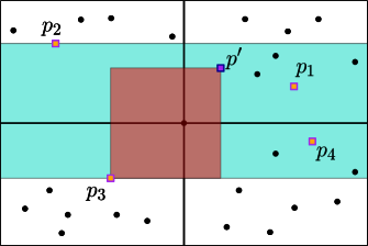
Figure 5.2: An illustration of Lemma 5.1. The lowest and highest points in the quadrants above and below the $x$-axis respectively are marked by $p_{i}$. In this case the pair of closest points of each side ($p_{1},p_{4}$) is not antipodal, and so the slab and the rightmost point in the slab are also shown, as well as the resulted rectangle.

 

Lemma 5.2.

The set $\mathcal{B}=\mathsf{bh}\left({P}\right)$ is connected. Furthermore, $\mathcal{B}$ is horizontally and vertically convex – formally, for any horizontal or vertical line $\ell$, either $\mathsf{bh}\left({P}\right)\cap\ell=\emptyset$, or it is a segment.

Proof:

We prove here that $\mathsf{bh}\left({P}\right)$ is vertically convex, as the horizontal case is similar. Let $p,q\in\mathsf{bh}\left({P}\right)$ be two points on some vertical line. If $p,q$ are both contained in some rectangle of $\mathcal{G}^{\vbox{\hbox{\scalebox{1.0}[0.5]{$\square$}}}}\left({P}\right)$ then we are done. Otherwise, we have two rectangles $\mathsf{b},\mathsf{d}\in\mathcal{G}^{\vbox{\hbox{\scalebox{1.0}[0.5]{$\square$}}}}\left({P}\right)$, such that $p\in\mathsf{b}$ and $q\in\mathsf{d}$, see Figure 5.3.

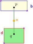
Figure 5.3:

Let $u$ be a point on the interior of the segment $pq$ that is outside $\mathsf{b}$ and $\mathsf{d}$. Without loss of generality, assume $u$ is the origin $(0,0)$. Since $u$ has $\mathsf{b}$ and $\mathsf{d}$ above and below it, it must be that the four points defining them in $P$ are in the four different quadrants of $u$.

If one of the points defining $\mathsf{b}$ and $\mathsf{d}$ has an $x$-value of $0$ we can assume that this point is in the quadrant not containing its counterpart for creating the appropriate rectangle. Lemma 5.1 implies that $u$ is contained in a rectangle of $\mathcal{G}^{\vbox{\hbox{\scalebox{1.0}[0.5]{$\square$}}}}\left({P}\right)$, and thus $u\in\mathsf{bh}\left({P}\right)$. A contradiction.  

Definition 5.3.

The ${\nearrow}$-maxima shadow, denoted by $\mathcal{S}\left({{\nearrow},P}\right)$, is the (closed) region in the plane of all points that dominates points in the ${\nearrow}$-maxima of $P$. The ${\nearrow}$-minima shadow ${\hskip 0.6pt\nwarrow}$-maxima shadow, and ${\nearrow}$-minima shadow, denoted respectively by $\mathcal{S}\left({{\swarrow},P}\right)$, $\mathcal{S}\left({{\hskip 0.6pt\nwarrow},P}\right)$, and ($\mathcal{S}\left({{\hskip 0.6pt\searrow},P}\right)$, are defined similarly. See Figure 5.4.

Observe that the shadow regions can be computed readily from the respective maxima/minima in linear time.

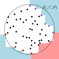
Figure 5.4:

Lemma 5.4.

Let $\mathcal{S}=\mathcal{S}\left({{\nearrow},P}\right)\cup\mathcal{S}\left({{\swarrow},P}\right)\cup\mathcal{S}\left({{\hskip 0.6pt\nwarrow},P}\right)\cup\mathcal{S}\left({{\hskip 0.6pt\searrow},P}\right)$. We have that $\mathsf{bh}\left({P}\right)=\mathrm{closure}(\mathbb{R}^{2}\setminus\mathcal{S})$.

Proof:

For simplicity of exposition we consider only points that are in the interior of the two sets. It is easy to verify that the argument can be modified to handle the boundary points.

Consider a point $q$ in the interior of $\mathcal{S}\left({{\nearrow},P}\right)\subseteq\mathbb{R}^{2}\setminus C$, where $C=\mathrm{closure}(\mathbb{R}^{2}\setminus\mathcal{S})$. The point $q$ dominates a point of $p$ that belongs to the maxima of $P$. It is straightforward to verify that any rectangle of $\mathcal{R}=\mathcal{R}^{\vbox{\hbox{\scalebox{1.0}[0.5]{$\square$}}}}\left({P}\right)$ that contains $q$, must also contain $p$, which contradicts $p$ being in the maxima. We conclude that $q\in\mathbb{R}^{2}\setminus\mathsf{bh}\left({P}\right)$. Applying the same argument to the other three shadows, readily implies that $\mathbb{R}^{2}\setminus C\subseteq\mathbb{R}^{2}\setminus\mathsf{bh}\left({P}\right)$, Namely, $\mathsf{bh}\left({P}\right)\subseteq C$.

Consider a point $q\in\mathrm{int}\left({C}\right)$. If the four quadrants of $q$ are all non-empty of points of $P$ then, by Lemma 5.1, $q\in\mathsf{bh}\left({P}\right)$. So assume that the top-right quadrant of $q$ is empty of points of $P$. This implies that $q$ appears in the interior of the ${\nearrow}$-maxima of $P\cup\{q\}$. In particular, there are two consecutive points $p_{1},p_{2}\in\mathsf{max}_{\nearrow}\left({P}\right)$, such that ${\mathsf{r}}={\vbox{\hbox{\scalebox{1.0}[0.5]{$\square$}}}\left({p_{1},p_{2}}\right)}\in\mathcal{R}$, and $q\in{\mathsf{r}}$. This readily implies that $q\in\mathsf{bh}\left({P}\right)$.  

5.1 Interior-disjoint cover of the box hull

Lemma 5.5.

Let $P$ be a set of $n$ points in the plane. One can compute, in $O(n\log n)$ time, a set $\mathcal{R}$ of $O(n)$ interior-disjoint rectangles of $\mathcal{G}^{\vbox{\hbox{\scalebox{1.0}[0.5]{$\square$}}}}\left({P}\right)$, such that $\cup\mathcal{R}=\mathsf{bh}\left({P}\right)$.

Proof:

Consider the following algorithm for constructing a set $\mathcal{R}^{\prime}$ of disjoint rectangles given a set $P$ of points. First, sort $P$ by increasing $x$-values. Given the sorted set, consider the points according to their ordering while maintaining two sorted sets, $C$ and $C^{\prime}$, that represent the ${\nearrow}$-maxima and ${\hskip 0.6pt\nwarrow}$-minima of the points seen so far, i.e. the top right and bottom right extremal staircases. Whenever a new point $p$ is inserted we can check in $O(\log n)$ time the set of points $P^{\prime}=\{p_{1},...,p_{m}\}$, sorted left to right, in $C$ or $C^{\prime}$ that, together with $p$, define edges in $\mathcal{G}^{\vbox{\hbox{\scalebox{1.0}[0.5]{$\square$}}}}\left({P}\right)$. Notice that $p$ must be either below $C$ or above $C^{\prime}$ depending on whether it is lower or higher than the last considered point, and thus one of $P^{\prime}\subseteq C$ or $P^{\prime}\subseteq C^{\prime}$ must be true. We now add ${\vbox{\hbox{\scalebox{1.0}[0.5]{$\square$}}}\left({p,p_{1}}\right)}$ to $\mathcal{R}$, and for every $i\in\{2,...,m\}$ we add the rectangle ${\vbox{\hbox{\scalebox{1.0}[0.5]{$\square$}}}\left({p,p_{i}}\right)}\setminus{\vbox{\hbox{\scalebox{1.0}[0.5]{$\square$}}}\left({p,p_{i-1}}\right)}$. Notice that due to the choice of points, this set of rectangles is pairwise disjoint, and is also disjoint from every other rectangle add to $\mathcal{R}^{\prime}$ thus far, as all previously added rectangles must reside below $C$, above $C^{\prime}$, and between consecutive points of $C$ and $C^{\prime}$. We now update $C$ and $C^{\prime}$ using $p$, i.e. replace $p_{1},...,p_{m}$ with $p$, or concatenate $p$ to the end of the chain, depending on $p$’s location with respect to the chain.

We are now left with proving the claimed properties of $\mathcal{R}$ other than disjointedness of interiors which has already been addressed. The size of $\mathcal{R}$ is straightforward to show as whenever a rectangle ${\vbox{\hbox{\scalebox{1.0}[0.5]{$\square$}}}\left({p,p_{i}}\right)}$ is added we either have that $p_{i}$ is the last point in $C$ and $C^{\prime}$ (i.e. the last point introduced before $p$), and after adding $p$ we still have $p_{i}$ on one of the chains, or $p_{i}$ was only a member of one of $C,C^{\prime}$, and was deleted when $p$ was inserted. The first option can only happen once, when $p_{i}$ is the last point in $C$ and $C^{\prime}$, and the second option can also happen only once as it results in the removal of $p_{i}$ from the data structure. This immediately implies an $O(n)$ size bound for $\mathcal{R}$.

The runtime of the algorithm is also fairly simple, as an addition of a point to the chains requires a constant number of comparisons and binary searches in the sets in order to find $p_{1},...,p_{m}$, after which the rectangles, which are computed in constant time each, are added. Since the number of rectangles is linear we get an $O(n\log n)$ runtime.

Now, let $p\in\bigcup\mathcal{R}$, without loss of generality $p=(0,0)$, and let $q,u$ be the rightmost points with negative $x$-value and positive and negative $y$-values respectively. Without loss of generality $x(u)<x(q)$. Denote the horizontal line through $q$ by $\ell$. If all of the points of $P$ to the right of $p$ are above $\ell$, then $p\notin\bigcup\mathcal{R}$, so let $v$ be the leftmost such point. Now, depending on whether $y(v)>0$ or $y(v)<0$ we have that when $v$ was added to the data structure, a rectangle covering $p$ was introduced to $\mathcal{R}$ due to $u$ or $q$ respectively. This proves that $\mathsf{bh}\left({P}\right)\subseteq\bigcup\mathcal{R}$, and since $\bigcup\mathcal{R}\subseteq\mathsf{bh}\left({P}\right)$ is evident from the algorithm we get $\mathsf{bh}\left({P}\right)=\bigcup\mathcal{R}$ as required.  

Remark 5.6.

Consider a point set $P$, informally, the convex-hull of $P$ can be defined by the repeated “closure” of $P$ under the process of adding segments to it, that connect two points of $P$ that do not have any point of $P$ in its interior. Similarly, the box hull can be defined analogously – the closure of the process of adding corners-induced “empty” rectangles to $P$.

Appendix A Chernoff’s inequality

Theorem A.1 ([MR95]).

Let $X_{1},...,X_{n}$ be $n$ independent random variables such that $X_{i}\in[0,1]$. Denote $Y=\sum_{i=1}^{n}X_{i}$, and $\mu=\mathop{\mathbf{E}}\!\left[{Y}\right]$. Then, we have

1. $\mathop{\mathbf{Pr}}\!\left[{Y\geq(1+\delta)\mu}\right]\leq\exp(-\delta^{2}\mu/4)$ for $\delta\in(0,4)$.

2. $\mathop{\mathbf{Pr}}\!\left[{Y\leq(1-\delta)\mu}\right]\leq\exp(-\delta^{2}\mu/2)$, for $\delta\in(0,1)$.

Appendix B Additional results

Here, we present some additional minor results.

B.1 Random points

The following claim is well known [Mul94].

Lemma B.1.

Let $P$ be a set of $n$ points picked uniformly, independently and randomly from $[0,1]^{2}$. Let $Y$ be the size of the maxima $\mathsf{max}_{\nearrow}\left({P}\right)$. We have that $\mathop{\mathbf{Pr}}\!\left[{Y>5\ln n}\right]\leq 1/n^{2}$ and $\mathop{\mathbf{Pr}}\!\left[{Y<(\ln n)/16}\right]\leq 1/n^{2/5}$.

Proof:

Sorting the points from right to left in decreasing $x$-coordinate values, the $i$th point has probability $1/i$ to be on the maxima of the first $i$ points, and these events are (somewhat surprisingly) independent [HR15, Lemma 3.3]. Thus, $\mu=\mathop{\mathbf{E}}\!\left[{Y}\right]=\sum_{i=1}^{n}1/i$. In particular $\ln n\leq\mu\leq\ln n+1$. By Chernoff’s inequality, Theorem A.1, we have

$$\mathop{\mathbf{Pr}}\!\left[{Y>5\ln n}\right]=\mathop{\mathbf{Pr}}\!\left[{Y>(1+4)\mu}\right]\leq\exp(-\mu 4^{2}/4)\leq 1/n^{4}.$$

Thus, the variable $Y$ is bounded by $5\ln n$ with high probability. Similarly, for $\delta=15/16$, by Chernoff’s inequality, we have

$$\mathop{\mathbf{Pr}}\!\left[{Y\leq(\ln n)/16}\right]\leq\mathop{\mathbf{Pr}}\!\left[{Y\leq(1-\delta)\mu}\right]\leq\exp(-\delta^{2}\mu/2)=\exp\Bigl{(}-\frac{225}{512}\mu\Bigr{)}\leq 1/n^{2/5}.$$

 

Lemma B.2.

Let $P$ be a set of points picked uniformly and independently from $[0,1]^{2}$. The number of edges in $\mathcal{G}=\mathcal{G}^{\vbox{\hbox{\scalebox{1.0}[0.5]{$\square$}}}}\left({P}\right)$ is $\Theta(n\log n)$ with high probability $1-O(1/n^{3/5})$.

Proof:

Let $p\in P$ be an arbitrary point of the set. we can use Lemma B.1 four times, once for every quadrant defined by $p$ in order to get an upper bound. Consider, say the points in the quadrant dominated by $p$, i.e. $P^{\prime}=P\cap\left\{q\in[0,1]^{2}\cap P\;\middle|\;q{\nearrow}p\right\}$. Since $|P^{\prime}|\leq n$ we have that $|\mathsf{max}_{\nearrow}\left({P^{\prime}}\right)|>5\ln n$ with probability at most $1/n^{2}$, and by using the claim for all four quadrants (with $\mathsf{max}_{\nearrow}\left({P}\right)$, $\mathsf{min}_{\nearrow}\left({P}\right)$, $\mathsf{max}_{\hskip 0.6pt\nwarrow}\left({P}\right)$ , or $\mathsf{min}_{\hskip 0.6pt\nwarrow}\left({P}\right)$ depending on the quadrant) we get that the probability that $p$ is incident to more than $20\ln n$ edges is at most $4/n^{2}$. Using the union bound immediately implies a probability of at least $1-4/n$ that every points is incident to $O(\ln n)$ edges in $\mathcal{G}^{\vbox{\hbox{\scalebox{1.0}[0.5]{$\square$}}}}\left({P}\right)$.

We now partition the unit square into nine squares $\square_{i,j}=[i/3,(i+1)/3]\times[j/3,(j+1)/3]$ for $i,j\in\{0,1,2\}$. The expected number of points, in each of these subsquares, is $\mu=n/9$, and

$$\mathop{\mathbf{Pr}}\!\left[{\left|{\square_{i,j}\cap P}\right|<n/18}\right]\leq\exp(-n/8),$$

by Chernoff’s inequality.

We therefore get that the probability that one of the nine squares contains less than $n/18$ points is $O(\exp(-n/8))$. Now, let $p\in P$ be a point in the center subsquare, i.e. $p\in\square_{1,1}=[1/3,2/3]\times[1/3,2/3]$. Each of the quadrants defined by $p$ fully contains a single subsquare $\square_{i,j}$, and therefore at least $n/18$ points. Denote $n^{\prime}=n/18$. Since the four quadrants are disjoint, we have by Lemma B.1 that the probability that the sizes of all the maxima and minima chains, of $p$, is smaller than $\ln n^{\prime}/16$ is smaller than

$$(1/n^{\prime 2/5})^{4}=(1/n^{\prime})^{8/5}=(18/n)^{8/5}.$$

The probability that any point, in the middle square, has less than $\ln n^{\prime}/16$ neighbors is therefore at most $O\bigl{(}\exp(-n/8)\bigr{)}+(n/18)(18/n)^{8/5}=O(1/n^{3/5})$ as required.  

Remark B.3.

The high probability bound, for the lower bound of Lemma B.2, is somewhat weak. It can be straightened by breaking the square into a constant size subsquares, argue that the RIG behavior inside each subsquare can be analyzed“independently”, and apply the bound of the lemma to each part. Thus showing that the number of edges of $\mathcal{G}$ complexity is $\Omega(n\log n)$ with probability $\geq 1-1/n^{O(1)}$.

B.2 The structure of $\mathcal{G}^{\vbox{\hbox{\scalebox{1.0}[0.5]{$\square$}}}}\left({P}\right)$

While $\mathcal{G}^{\vbox{\hbox{\scalebox{1.0}[0.5]{$\square$}}}}\left({P}\right)$ can have a quadratic number of edges, it is fairly straightforward to see that it does not have $K_{5}$ as a subgraph, as Dilworth’s Theorem guarantees the existence of a ${\nearrow}$ or ${\hskip 0.6pt\nwarrow}$-chain of size three for any set of five points in general position, but if say $p{\nearrow}q{\nearrow}u$ we have $q\in{\vbox{\hbox{\scalebox{1.0}[0.5]{$\square$}}}\left({p,u}\right)}$ which means $pu\notin\mathcal{G}^{\vbox{\hbox{\scalebox{1.0}[0.5]{$\square$}}}}\left({P}\right)$. In this section we show that not only does $\mathcal{G}^{\vbox{\hbox{\scalebox{1.0}[0.5]{$\square$}}}}\left({P}\right)$ not contain large cliques, it also does not contain large tricliques, i.e. disjoint triplets $R,G,B\subseteq P$ such that every pair of points from different sets are connected by an edge in $\mathcal{G}^{\vbox{\hbox{\scalebox{1.0}[0.5]{$\square$}}}}\left({P}\right)$. This means that the graph owes its size to the existence of large bicliques. In the following we analyze the structure of $\mathcal{G}^{\vbox{\hbox{\scalebox{1.0}[0.5]{$\square$}}}}\left({P}\right)$ as discussed above, and give bounds on its size in the case that $P$ is a set of uniformly distributed random points.

B.2.1 Bicliques and tricliques in $\mathcal{G}^{\vbox{\hbox{\scalebox{1.0}[0.5]{$\square$}}}}\left({P}\right)$

Formally, a triclique over disjoint sets $X,Y,Z$ is the graph $(X\otimes Y)\cup(X\otimes Z)\cup(Y\otimes Z)$.

Lemma B.4.

Let $P\subseteq\mathbb{R}^{2}$ be a set of $n$ points. If $\mathcal{G}^{\vbox{\hbox{\scalebox{1.0}[0.5]{$\square$}}}}\left({P}\right)$ contains $K_{k,k}$, where $k>4$, as a subgraph, then either $\mathcal{G}^{\vbox{\hbox{\scalebox{1.0}[0.5]{$\square$}}}}_{\hskip 0.6pt\nwarrow}\left({P}\right)$ or $\mathcal{G}^{\vbox{\hbox{\scalebox{1.0}[0.5]{$\square$}}}}_{\nearrow}\left({P}\right)$ contain the biclique $K_{k,k-4}$ as a subgraph, formed by two or three chains, one of which is of length $k$.

Proof:

Denote the biggest biclique in $\mathcal{G}^{\vbox{\hbox{\scalebox{1.0}[0.5]{$\square$}}}}\left({P}\right)$ by $C=B\otimes R$. We will refer to the points in $B$ and $R$ as the red and blue points. Let $C_{b}=(b_{1},...,b_{m})$ be the longest ${\nearrow}$-chain/anti-chain in $G$. We assume without loss of generality that $C_{b}$ is a ${\nearrow}$-antichain of blue points, and notice that since $k>4$ we have $m>2$ (Dilworth’s Theorem). The axis parallel lines through $b_{1}$ and $b_{m}$ partition $\mathbb{R}^{2}$ into 9 parts $M_{1,1},...,M_{3,3}$, where $M_{1,1}$ is above and to the left of $b_{1}$, and $M_{3,3}$ is below and to the right of $b_{k}$. See Figure B.1 for an illustration.

$M_{1,1}$ and $M_{3,3}$ cannot contain any point of $C$ since blue points would break the maximality assumption on $C_{b}$, and red points would not be connected by an edge to both $b_{1}$ and $b_{m}$.

Denote the downward generalized chain of $C_{b}$ by $C_{b}^{\prime}$. Assume without loss of generality that at least $\frac{|R|}{2}$ of the red points are in the downward generalized quadrant of $C_{b}$, i.e. below $C_{b}^{\prime}$ and in the union of $M_{2,1},M_{3,1}$, and $M_{3,2}$, as $M_{3,3}$ does not contain any red or blue point, and let $C_{r}=(r_{1},...,r_{l})$ be the longest anti-chain of red points in that generalized quadrant.

We now notice that any red point below $C_{b}^{\prime}$ that is not a part of $C_{r}$ either prevents a point on $C_{r}$ from connecting to a point on $C_{b}$, or cannot connect to a point of $C_{b}$ because of a point in $C_{r}$. More precisely, for any two points $p,q$ below $C_{b}^{\prime}$, if $p{\nearrow}q$, then, for any $1\leq i\leq m$, it is not possible that ${\vbox{\hbox{\scalebox{1.0}[0.5]{$\square$}}}\left({p,b_{i}}\right)}$ does not contain points of $P$ in their interior. We therefore get that for every such pair of points either $p{\hskip 0.6pt\nwarrow}q$, or $q{\hskip 0.6pt\nwarrow}p$, and thus all of the red points bellow $C_{b}^{\prime}$ are in $C_{r}$, meaning $|C_{r}|\geq\frac{k}{2}$, and since $|C_{b}|\geq|C_{r}|$ by assumption, we get that $|C_{b}|\geq\frac{k}{2}$.

Also, no point of $R$ can anti-dominate or be anti-dominated by more than one point of $C_{b}$. Furthermore, for a point to be connected to all of $C_{b}$’s point by an edge in $\mathcal{G}^{\vbox{\hbox{\scalebox{1.0}[0.5]{$\square$}}}}\left({P}\right)$, and anti-dominate or be anti-dominated by a point of $C_{b}$, that point must be in $M_{2,1},M_{2,2},$ or $M_{3,2}$. See Figure B.1. If a red point $r$ exists in $M_{2,2}$, then it must be the case that $b_{1}{\hskip 0.6pt\nwarrow}r$, and $r{\hskip 0.6pt\nwarrow}b_{m}$. In that case no other red point exists below $C_{b}^{\prime}$, as no other point can connect to all of the points of $C_{b}$ with an edge. Since $k>4$ and $|C_{r}|\geq\frac{|R|}{2}$ we have that $M_{2,2}$ does not have any points of $P\setminus C_{b}$ below $C_{b}^{\prime}$.

$M_{2,1}$ and $M_{3,2}$ can only contain one red point each since there is no way to place two points in either cells that allows both points to connect to all of $C_{b}$ with an edge. If, say, $M_{2,3}$ contains a red point $r$, then it must be the case that $r{\hskip 0.6pt\nwarrow}b_{m}$, and $b_{i}{\nearrow}r$ for every $1\leq i<m$. The case where a red point exists in $m_{3,2}$ is similar. We thus have that $|C_{r}|-2$ of the red points below $C_{b}^{\prime}$ are in $M_{3,3}$, and these points create, together with $C_{b}$, ${\hskip 0.6pt\nwarrow}$-chains forming a biclique in $\mathcal{G}^{\vbox{\hbox{\scalebox{1.0}[0.5]{$\square$}}}}_{\nearrow}\left({P}\right)$ of size at least as big as $K_{\frac{k}{2},\frac{k}{2}-2}$.

If there are no red points above $C_{b}^{\prime}$, then we actually get that $|C_{r}|=k$, and thus $|C_{b}|\geq|C_{r}|=k$ as well, which implies a $K_{k,k-2}$ biclique in $\mathcal{G}^{\vbox{\hbox{\scalebox{1.0}[0.5]{$\square$}}}}_{\nearrow}\left({P}\right)$ formed by two ${\hskip 0.6pt\nwarrow}$-chains of length $k$. Otherwise we notice that if a blue point $b$ is placed in $M_{2,1}$ or $M_{3,2}$, which can be done in a way that allows an edge between it and the single red point that might be in $M_{1,2}$ or $M_{2,3}$, $b$ can neither dominate or anti-dominate any point of $C_{r}$, as that would not allow the red point to connect to some points of $C_{b}$, and so it must be dominated or anti dominated by them. However, this is only possible if $|R|=k\leq 2$, as $b$ can be connected by an edge to at most two points of the ${\hskip 0.6pt\nwarrow}$-chain $C_{r}$ if it is “between” them in $M_{3,1}$, or a single one if it is in $M_{2,1}$ or $M_{3,2}$. For similar reasons blue points can not be placed above $C_{b}$ unless $C_{r}$ is a single point in $M_{2,1}\cup M_{3,2}$. This means that $C_{b}=B$. Now we can use the same arguments used for $C_{r}$ to show that the red points above $C_{b}^{\prime}$ form an anti-chain, and that at most two of them can exist outside of $M_{1,3}$. In this case the three anti-chains (two red and one blue) form a $K_{k,k-4}$ biclique in $\mathcal{G}^{\vbox{\hbox{\scalebox{1.0}[0.5]{$\square$}}}}_{\nearrow}\left({P}\right)$, formed by 3 ${\hskip 0.6pt\nwarrow}$-chains, one of which is of length $k$.

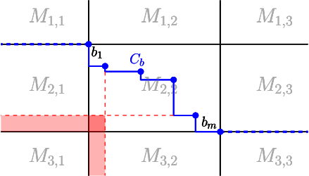
Figure B.1: An illustration of the longest chain, and the partition it induces on $\mathbb{R}^{2}$. The ${\nearrow}$-antichain $C_{b}$ is shown as a blue axis-parallel curve, the generalized ${\nearrow}$-antichain $C_{b}^{\prime}$ is shown as the continuation of $C_{b}$ with dashed blue lines, and the region of $M_{2,1}\cup M_{2,2}\cup M_{3,2}$ that can contain red points is shown in red.

 

Corollary B.5.

For a triclique $\{R,B,G\}$ in $\mathcal{G}^{\vbox{\hbox{\scalebox{1.0}[0.5]{$\square$}}}}\left({P}\right)$ such that $|R|\leq|B|\leq|G|$, we must have $|G|=1$.

Proof:

Since the proof is similar in flavor to that of Lemma B.4 in that it is a case analysis over the partition of the plane induced by the participating points, we use a simple proof by drawing using Figure B.2. First we notice that the structure described in Lemma B.4 does not require that $k>4$ for anything but the size of a one directional biclique, and all of the arguments apply when $k\geq 3$. We therefore get that if $|B|\geq 3$ then the biclique $\{R,B\}$ includes, without loss of generality, an ${\hskip 0.6pt\nwarrow}$-chain of three points of $R$, and an ${\hskip 0.6pt\nwarrow}$-chain of two points of $B$.

In the figure we have an ${\hskip 0.6pt\nwarrow}$-chain of size three of $R$, and an ${\hskip 0.6pt\nwarrow}$-chain of size two of $B$ which must exist due to arguments in Lemma B.4. Notice that regardless of the position of the two blue points in the partition induced by the red points, there are no regions in which more than one point of $G$ can be added in order to form a triclique. The areas are coded to show the reason why a point of $G$ cannot be placed in that region; red if it cannot connect with an edge of $\mathcal{G}^{\vbox{\hbox{\scalebox{1.0}[0.5]{$\square$}}}}\left({P}\right)$ to all points of $R$, blue if it cannot connect to all points of $B$, purple if it prevents a point of $R$ and a point of $B$ from connecting, and a tiling pattern if it can only be connected to two or less blue points. Note that blue points cannot be placed in red regions and vice versa.  

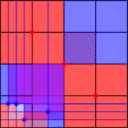
Figure B.2: A color and texture coded map of the proof for the size of tricliques in $\mathcal{G}^{\vbox{\hbox{\scalebox{1.0}[0.5]{$\square$}}}}\left({P}\right)$

B.3 Approximating independent set of rectangles

Lemma B.6.

Let $\mathcal{R}=\left\{{\vbox{\hbox{\scalebox{1.0}[0.5]{$\square$}}}\left({p,q}\right)}\;\middle|\;pq\in\mathcal{G}^{\vbox{\hbox{\scalebox{1.0}[0.5]{$\square$}}}}\left({P}\right)\right\}$, and let $I$ be

$$\underset{X\subseteq\mathcal{R}}{\mathsf{argmax}}\left\{|X|\;\middle|\;\forall\mathsf{b},\mathsf{d}\in X,\mathsf{b}\cap\mathsf{d}=\emptyset\right\},$$

i.e. $I$ is a maximum size independent set of rectangles giving rise to edges of $\mathcal{G}^{\vbox{\hbox{\scalebox{1.0}[0.5]{$\square$}}}}\left({P}\right)$. It is possible, in $O(n\log^{2}n)$ time, to find an independent set of $\mathcal{R}$ of size $\Omega(|I|/\log n)$.

Proof:

The proof here is similar to that of Lemma 4.1, and we will therefore only describe the algorithm for finding a maximum size independent set of rectangles of $\mathcal{G}^{\vbox{\hbox{\scalebox{1.0}[0.5]{$\square$}}}}\left({P}\right)$ intersecting a vertical line $\ell$. Since we can only take one rectangle from every biclique we traverse the biclique cover and keep, from every biclique that intersects $\ell$, only the rectangle created by the lowest point in $P_{i}$ and the highest point in $Q_{1}$, assuming that $P_{i}$ is above $Q_{i}$ (remember they are quadrant separated by Observation 3.9). We then return the maximum independent set of intervals corresponding to the projections of these rectangle on $\ell$. The number of rectangles is $O(n)$, and thus we can get the maximum independent set in $O((n\log n)$ time using a greedy algorithm for maximum interval independent set.

The rest of the proof, i.e. recursive algorithm and runtime analysis is similar to that of Lemma 4.1, with the small differences of considering the sum of sets in each level of the recursion when keeping track of the maximum value, and the runtime itself which is dominated by the construction of the cover rather than the one-dimensional algorithm and thus results in an $O(n\log^{3}n)$ overall runtime.  

B.4 Induced subgraphs and edges

Lemma B.7.

For a set $P\subseteq\mathbb{R}^{2}$ of $n$ points in the plane, if $P$ does not contain a ${\nearrow}$-chain or anti-chain of length $l$, then $\mathcal{G}^{\vbox{\hbox{\scalebox{1.0}[0.5]{$\square$}}}}\left({P}\right)$ contains $K_{k,k}$ as an induced subgraph for some $k=O(n/l)$.

Proof:

We first partition $\mathbb{R}^{2}$ into four quadrants, such that two antipodal quadrants contain at least $n/4$ points of $P$ each. This can be done by finding a horizontal line that separates $P$ into two sets of equal size ($\pm 1$), and then finding a vertical line with minimal $x$-coordinate that contains $n/4$ points of one of the halves to its left.

We now consider the two quadrants, without loss of generality these are the positive and negative quadrants (i.e. $(+,+)$ and $(-,-)$ quadrants respectively) denoted $\mathcal{Q}_{1}$ and $\mathcal{Q}_{3}$, and denote $P^{+}=\mathcal{Q}_{1}\cap P$ and $P^{-}=\mathcal{Q}_{3}\cap P$ . By Dilworth’s Theorem, since the longest ${\nearrow}$-chain, in each quadrant is of length at most $l$, there is a partitioning of $P^{+}$ and $P^{-}$ number into $l$ mutually disjoint ${\nearrow}$-antichains. The largest ${\nearrow}$-antichain in each of these sets is of length $\geq\frac{n}{4l}$, and the induced RIG over the set of points constituting these anti-chains is there $K_{k,k^{\prime}}$ for $k,k^{\prime}\geq\frac{n}{4l}$.  

Lemma B.8.

Let $R$ be the set of all rectangles defined by points of $P$ (regardless of the number of points of $P$ in their interior). There exists a point $p\in\mathbb{R}^{2}$ that is contained in $O(n/2)$ rectangles of $R$ such that no two rectangles are supported by the same point, i.e. the set of points supporting the rectangles is $P$. Furthermore we can find such a point in $O(n)$ time.

Proof:

We start by finding a vertical line $\ell_{v}$ that splits the points of $P$ into two parts of equal size. Let $P_{0}=P$, and let $x^{+}$ and $x^{-}$ be two counters initialized to 0. In the $i$th iteration we find a horizontal line $\ell^{i}_{h}$ that splits $P_{i-1}$ into two parts of equal size, let $P_{i}^{+}$ be the points of $P_{i-1}$ above $\ell_{h}$ and to the right of $\ell_{v}$, and let $P_{i}^{-}$ be the points of $P_{i-1}$ below $\ell_{h}$ and to the left of $\ell_{v}$. if $P_{i}^{+}+x^{+}=P_{i}^{-}+x^{-}$ we return the intersection point of $\ell_{v}$ and $\ell^{i}_{h}$, otherwise without loss of generality that $P_{i}^{+}+x^{+}>P_{i}^{-}+x^{-}$. We set $x^{-}=x^{-}+|P_{i}^{-}|$, and $P_{i}=P_{i-1}\setminus\left\{p\in P\;\middle|\;p\text{ is below }\ell^{i}_{h}\right\}$.

The correctness follows the simple observation that the process will always terminate when every two antipodal quadrants created by the lines will contain the same number of points in each quadrant. The runtime is given by the recursive formula $T(n)=T(n/2)+O(n)$ using linear time median selection. The formula gives an overall linear runtime.

References

- [ADH14] Boris Aronov, Muriel Dulieu and Ferran Hurtado “Witness Rectangle Graphs” In Graphs Comb. 30.4, 2014, pp. 827–846 DOI: 10.1007/s00373-013-1316-x
- [AEGR12] Deepak Ajwani, Khaled M. Elbassioni, Sathish Govindarajan and Saurabh Ray “Conflict-Free Coloring for Rectangle Ranges Using O(n .382) Colors” In Discrete Comput. Geom. 48.1, 2012, pp. 39–52 DOI: 10.1007/s00454-012-9425-5
- [AFK85] Noga Alon, Zoltán Füredi and Meir Katchalski “Separating Pairs of Points by Standard Boxes” In Eur. J. Comb. 6.3, 1985, pp. 205–210 DOI: 10.1016/S0195-6698(85)80028-7
- [BBM99] Therese C. Biedl, Anna Bretscher and Henk Meijer “Rectangle of Influence Drawings of Graphs without Filled 3-Cycles” Stirín Castle, Czech Republic In Proc. 7th Int. Symp. Graph Draw. (GD) 1731, Lect. Notes in Comp. Sci. Springer, 1999, pp. 359–368 DOI: 10.1007/3-540-46648-7“˙37
- [BCO92] Mark Berg, Svante Carlsson and Mark H. Overmars “A General Approach to Dominance in the Plane” In J. Algorithms 13.2, 1992, pp. 274–296 DOI: 10.1016/0196-6774(92)90019-9
- [BS07] B. Bollobás and A. Scott “On separating systems” In Eur. J. Comb. 28.4, 2007, pp. 1068–1071
- [BS80] Jon Louis Bentley and James B. Saxe “Decomposable Searching Problems I: Static-to-Dynamic Transformation” In J. Algorithms 1.4, 1980, pp. 301–358 DOI: 10.1016/0196-6774(80)90015-2
- [Cha12] Timothy M. Chan “Conflict-free coloring of points with respect to rectangles and approximation algorithms for discrete independent set” In Proc. 28th Annu. Sympos. Comput. Geom. (SoCG) ACM, 2012, pp. 293–302 DOI: 10.1145/2261250.2261293
- [CPST09] Xiaomin Chen, János Pach, Mario Szegedy and Gábor Tardos “Delaunay graphs of point sets in the plane with respect to axis-parallel rectangles” In Random Struct. Algorithms 34.1, 2009, pp. 11–23 DOI: 10.1002/RSA.20246
- [ELL+94] Hossam A. ElGindy et al. “Recognizing Rectangle of Influence Drawable Graphs” In Graph Drawing, DIMACS International Workshop, GD ’94, Princeton, New Jersey, USA, October 10-12, 1994, Proceedings 894, Lecture Notes in Computer Science Springer, 1994, pp. 352–363 DOI: 10.1007/3-540-58950-3“˙390
- [GNO89] Ralf Hartmut Güting, Otto Nurmi and Thomas Ottmann “Fast Algorithms for Direct Enclosures and Direct Dominances” In J. Algorithms 10.2, 1989, pp. 170–186 DOI: 10.1016/0196-6774(89)90011-4
- [HR15] Sariel Har-Peled and Benjamin Raichel “On the Complexity of Randomly Weighted Multiplicative Voronoi Diagrams” In Discrete Comput. Geom. 53.3, 2015, pp. 547–568 DOI: 10.1007/s00454-015-9675-0
- [HS05] Sariel Har-Peled and Shakhar Smorodinsky “Conflict-Free Coloring of Points and Simple Regions in the Plane” In Discrete Comput. Geom. 34.1, 2005, pp. 47–70 DOI: 10.1007/s00454-005-1162-6
- [IS85] Manabu Ichino and Jack Sklansky “The relative neighborhood graph for mixed feature variables” In Pattern Recognit. 18.2, 1985, pp. 161–167 DOI: 10.1016/0031-3203(85)90040-8
- [LLMW98] Giuseppe Liotta, Anna Lubiw, Henk Meijer and Sue Whitesides “The rectangle of influence drawability problem” In Comput. Geom. 10.1, 1998, pp. 1–22 DOI: 10.1016/S0925-7721(97)00018-7
- [MMN09] Kazuyuki Miura, Tetsuya Matsuno and Takao Nishizeki “Open Rectangle-of-Influence Drawings of Inner Triangulated Plane Graphs” In Discret. Comput. Geom. 41.4, 2009, pp. 643–670 DOI: 10.1007/s00454-008-9098-2
- [MN05] Kazuyuki Miura and Takao Nishizeki “Rectangle-of-Influence Drawings of Four-Connected Plane Graphs” In Asia-Pacific Symposium on Information Visualisation, APVIS 2005, Sydney, Australia, January 27-29, 2005 45, CRPIT Australian Computer Society, 2005, pp. 75–80 URL: http://crpit.scem.westernsydney.edu.au/abstracts/CRPITV45Miura.html
- [MOW87] J. Munro, Mark H. Overmars and Derick Wood “Variations on Visibility” In Proceedings of the Third Annual Symposium on Computational Geometry, Waterloo, Ontario, Canada, June 8-10, 1987 ACM, 1987, pp. 291–299 DOI: 10.1145/41958.41989
- [MR95] Rajeev Motwani and Prabhakar Raghavan “Randomized Algorithms” Cambridge University Press, 1995 DOI: 10.1017/cbo9780511814075
- [Mul94] K. Mulmuley “Computational Geometry: An Introduction Through Randomized Algorithms” Englewood Cliffs, NJ: Prentice Hall, 1994 URL: http://www.amazon.com/Computational-Geometry-Introduction-Randomized-Algorithms/dp/0133363635
- [OW88] Mark H. Overmars and Derick Wood “On Rectangular Visibility” In J. Algorithms 9.3, 1988, pp. 372–390 DOI: 10.1016/0196-6774(88)90028-4
- [SZ10] Sadish Sadasivam and Huaming Zhang “Closed Rectangle-of-Influence Drawings for Irreducible Triangulations” In Theory and Applications of Models of Computation, 7th Annual Conference, TAMC 2010, Prague, Czech Republic, June 7-11, 2010. Proceedings 6108, Lecture Notes in Computer Science Springer, 2010, pp. 409–418 DOI: 10.1007/978-3-642-13562-0“˙37
- [Tou80] Godfried T. Toussaint “The relative neighbourhood graph of a finite planar set” In Pattern Recognit. 12.4, 1980, pp. 261–268 DOI: 10.1016/0031-3203(80)90066-7
- [ZV09] Huaming Zhang and Milind Vaidya “On Open Rectangle-of-Influence Drawings of Planar Graphs” Huangshan, China, June 10-12 In Proc. Comb. Opt. Appl., 3rd Int. Conf. (COCOA) 5573, Lect. Notes in Comp. Sci. Springer, 2009, pp. 123–134 DOI: 10.1007/978-3-642-02026-1“˙11