Minimum Star Partitions of Simple Polygons in Polynomial Time

Abstract

We devise a polynomial-time algorithm for partitioning a simple polygon $P$ into a minimum number of star-shaped polygons. The question of whether such an algorithm exists has been open for more than four decades [Avis and Toussaint, Pattern Recognit., 1981] and it has been repeated frequently, for example in O’Rourke’s famous book [Art Gallery Theorems and Algorithms, 1987]. In addition to its strong theoretical motivation, the problem is also motivated by practical domains such as CNC pocket milling, motion planning, and shape parameterization.

The only previously known algorithm for a non-trivial special case is for $P$ being both monotone and rectilinear [Liu and Ntafos, Algorithmica, 1991]. For general polygons, an algorithm was only known for the restricted version in which Steiner points are disallowed [Keil, SIAM J. Comput., 1985], meaning that each corner of a piece in the partition must also be a corner of $P$. Interestingly, the solution size for the restricted version may be linear for instances where the unrestricted solution has constant size. The covering variant in which the pieces are star-shaped but allowed to overlap—known as the Art Gallery Problem—was recently shown to be $\exists\mathbb{R}$-complete and is thus likely not in NP [Abrahamsen, Adamaszek and Miltzow, STOC 2018 & J. ACM 2022]; this is in stark contrast to our result. Arguably the most related work to ours is the polynomial-time algorithm to partition a simple polygon into a minimum number of convex pieces by Chazelle and Dobkin [STOC, 1979 & Comp. Geom., 1985].

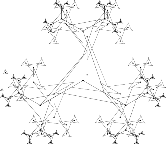
Figure 1: Repeating the patterns, we obtain polygons where star centers and corners of pieces of arbitrarily high degree are required.

1 Introduction

A simple polygon $Q$ is called star-shaped if there is a point $A$ in $Q$ such that for all points $B$ in $Q$, the line segment $AB$ is contained in $Q$. Such a point $A$ is called a star center of $Q$. A star partition of a polygon $P$ is a set of pairwise non-overlapping star-shaped simple polygons whose union equals $P$; see Figure 1. The polygons constituting the star partition are called the pieces of the partition.

Avis and Toussaint [AT81] described in 1981, an algorithm running in $O(n\log n)$ time to partition a simple polygon (i.e., a polygon without holes) into at most $\lfloor n/3\rfloor$ star-shaped pieces—where $n$ denotes the number of corners of the polygon—based on Fisk’s constructive proof [Fis78] of Chvátal’s Art Gallery Theorem [Chv75]. Avis and Toussaint [AT81] wrote: “An interesting open problem would be to try to find the decomposition into the minimum number of star-shaped polygons.” This question has been repeated in several other papers [Tou82, OS83, Kei85, She92] and also in O’Rourke’s well-known book [ORo87]: “Can a variant of Keil’s dynamic programming approach [Kei85] be used to find star partitions permitting Steiner points? Chazelle was able to achieve $O(n^{3})$ for minimum convex partition with Steiner points via a very complex dynamic programming algorithm [Cha80], but star partitions seem even more complicated.” Before our work, the problem was not known to be in NP and not even an exponential-time algorithm was known. In this paper, we resolve the open problem by providing a polynomial-time algorithm, thereby closing a research question that has been open for more than four decades.

theoremMainTheorem There is an algorithm with running time $O(n^{107})$ that partitions a simple polygon with $n$ corners into a minimum number of star-shaped pieces.

Related work.

The minimum star partition problem belongs to the class of decomposition problems, which forms an old and large sub-field in computational geometry. In all of these problems, we want to decompose a polygon $P$ into polygonal pieces which are in some sense simpler than the original polygon $P$. Here, the union of the pieces should be $P$, and we usually seek a decomposition into as few pieces as possible. A decomposition where the pieces may overlap is called a cover, and a decomposition where the pieces are pairwise interior-disjoint is called a partition. This leads to a wealth of interesting problems, depending on the assumptions about the input polygon $P$ and the requirements on the pieces. There is a vast literature about such decomposition problems, as documented in several highly-cited books and survey papers that give an overview of the state-of-the-art at the time of publication [KS85, Cha87, ORo87, She92, CP94, Kei99, OST18]. Some of the most common variations are

• whether the input polygon $P$ is simple or may have holes,

• whether we seek a cover or a partition,

• whether we allow Steiner points${}^{\text{\ref{footnote:steiner-points}}}$ or not,

• what shape of pieces we allow; let us mention that for partitioning a simple polygon, variants have been studied with polygonal pieces that are convex [FP75, Sch78, CD85, Kei85, Cha82, HM85, KS02], star-shaped [FP75, Kei85, LN91], monotone [GJP+78, LN88], spiral-shaped [Kei85], “fat” [Kre98, Dam04, BS21], “small” [ADG+20, DP04], “circular” [DO03], triangles [AAP86, Cha91], quadrilaterals [Lub85, MW97] and trapezoids [AAI86].

Closely related to our problem is that of covering a polygon with a minimum number of star-shaped pieces. This is usually known as the Art Gallery Problem and described equivalently as the task of placing guards (star centers) so that each point in the polygon can be seen by at least one guard. Interestingly, the Art Gallery Problem has been shown to be $\exists\mathbb{R}$-complete [AAM22] and it is thus not likely to be in NP. This is in stark contrast to our main result, which shows that the corresponding partitioning problem is in P. Covering a polygon with a minimum number of convex pieces is likewise $\exists\mathbb{R}$-complete [Abr21].

If the polygon $P$ can have holes, the minimum star partition problem is known to be NP-hard, whether or not Steiner points are allowed [ORo87]; again in contrast to our result.

Keil [Kei85] gave polynomial-time algorithms for partitioning simple polygons into various types of pieces where Steiner points are not allowed. Among these algorithms is an $O(n^{7}\log n)$ time algorithm for finding a minimum star partition of a simple polygon without Steiner points, but the unrestricted version of the problem (with Steiner points allowed) remained open. Let us mention that there are polygons where $\Theta(n)$ pieces are needed when Steiner points are not allowed, whereas $2$ pieces are sufficient when they are allowed; see Figure 2 (left). Therefore, our algorithm in general constructs partitions that are significantly smaller. This highlights an interesting difference between minimum star partitions and convex partitions: A minimum convex partition without Steiner points has at most $4$ times as many pieces as when Steiner points are allowed [HM85]. Another difference is that an arbitrarily small perturbation of a single corner can change the size of the minimum star partition between $1$ and $\Theta(n)$, whereas the change in size of the minimum convex partition is at most $1$; see Figure 2 (right). In that sense, minimum star partitions are much more sensitive to the input.

Figure 2: Left: A polygon that is partitioned into two star-shaped pieces using the Steiner point $S$. A star center that can see the two middle groups of spikes must be placed at or close to $A_{1}$, while a star center that sees the outer groups must be at or close to $A_{2}$. Without Steiner points we need $\Theta(n)$ pieces to partition at least one of the groups of spikes. Right: Moving the bottom corner a bit up changes the size of a minimum star partition from $1$ to $\Theta(n)$.

Unrestricted partitioning problems (that is, allowing Steiner points), are seemingly much more challenging to design algorithms for. Chazelle and Dobkin [Cha80, CD85] proved already in 1979 that a simple polygon can be partitioned into a minimum number of convex pieces in $O(n^{3})$ time, by designing a rather complicated dynamic program. Asano, Asano and Imai [AAI86] gave an $O(n^{2})$-time algorithm for partitioning a simple polygon into a minimum number of trapezoids, each with a pair of horizontal edges. However, the minimum partitioning problem has remained open for most other shapes of pieces (e.g. triangles, spiral-shaped, and—until now—star-shaped).

Liu and Ntafos [LN91] also studied the minimum star partition problem, but with restrictions on the input polygon. They describe an algorithm for partitioning simple monotone and rectilinear polygons into a minimum number of star-shaped polygons in $O(n)$ time, and a $6$-approximation algorithm for simple rectilinear polygons that are not necessarily monotone.

Challenges.

As argued above, star partitions are very sensitive to the input polygon, and allowing Steiner points is in general necessary to obtain a partition with few pieces (Figure 2). In order to demonstrate the complicated nature of optimal star partitions, let us also consider Figure 1, which shows (representatives of) two families of polygons with arbitrarily many corners and unique optimal star partitions. In both examples, some star centers and Steiner points depend on as many as $\Theta(n)$ corners of $P$. The example to the right shows that star centers and Steiner points of degree $\Theta(n)$ are also needed, where points $V_{i}$ of degree $i$ are defined as follows. The points $V_{0}$ are the corners of $P$; and $V_{i+1}$ are the intersection points between two non-parallel lines, each through a pair of points in $V_{i}$. The size of $V_{i}$ grows as $\Theta(n^{4^{i}})$, so we cannot iterate through the possible star centers and Steiner points. This is in contrast to the problem without Steiner points studied by Keil [Kei85]. Here, by definition, the corners of the pieces are in $V_{0}$ and it is not hard to see that the star centers can be chosen from $V_{1}$, of which there are “only” $O(n^{4})$.

Since we cannot iterate through all possible star centers and Steiner points, we devise a two-phase algorithm, as follows. In the first phase, we find polynomially many relevant points, so that we are sure that an optimal solution can be constructed using a subset of those points as star centers and Steiner points. In the second phase, we use dynamic programming to find optimal solutions to larger and larger subpolygons, using only the constructed points from the first phase. We note however that the phases are intertwined as the algorithm for the first phase calls the complete partitioning algorithm recursively on subpolygons. The argument that the set of points constructed in the first phase is sufficient relies on several structural results about optimal star partitions which we believe are interesting in their own right.

1.1 Practical Motivation

Besides being interesting from a theoretical angle, star partitions are useful in various practical domains; below we mention a few examples. Many of the papers mentioned below describe algorithms for computing star partitions with no guarantee of finding an optimal one.

CNC pocket milling.

Our first motivation comes from the generation of toolpaths for milling machines. CNC milling is the computer-aided process of cutting some specified shape into a piece of material—such as steel, wood, ceramics, or plastic—using a milling machine. When milling a pocket, spirals are a popular choice of toolpath, since the entire pocket can be machined without retracting the tool and sharp corners on the path can be largely avoided. Some of the proposed methods to generate spirals require the shape of the pocket to be star-shaped, for instance because they rely on radial interpolation between curves that morph a single point (a star center) to the boundary of the pocket [BS03, PL19, BFB12]. When milling a non-star-shaped pocket, we therefore seek to first partition the pocket into star-shaped regions, each of which can then be milled by their own spiral. We want a star partition rather than a star cover, since it is a waste of time to cover the same area more than once. In order to minimize the number of retractions (lifting and moving the tool from one spiral to the next), we want a partition into a minimum number of star-shaped regions.

Motion planning.

Star partitions are also useful in the domain of motion planning. Varadhan and Manocha [VM05] describe such an approach. They first partition the free space into star-shaped regions to subsequently construct a route for an agent from one point to another in the free space using the stars. In each star, we route from the point of entrance to the star center and from there to a common boundary point with the next star. Similar applications of star partitions are described in [DKB13, Lie07, LL09, ZKV+06].

Capturing the shape of a polygon.

Star partitions can be used to blend/morph one polygon into another [SR95, ER97], for shape matching and retrieval [YL11], and they are also used in shape parameterization [XHH+10].

1.2 Technical Overview

To enable our algorithm, we had to identify a multitude of interesting structural properties of optimal star partitions, which are interesting in their own right. In this section, we outline the most important of these properties and explain informally how they are used to derive a polynomial-time algorithm. Naturally, we sometimes stay vague or glance over complicated details in order to hide complexity to make the technical overview easily accessible.

Figure 3: Left: A polygon with a star partition and an example of a short (orange) and a long (green) separator. Right: The dual graph of the partition. The short and long separators of the partition correspond to vertices, respectively edges, in the graph.

Separators.

Similar to the algorithms for related partitioning problems [CD85, Kei85], we use dynamic programming: We compute optimal star partitions of larger and larger subpolygons $P^{\prime}$ contained in the input polygon $P$. For dynamic programming to work, we need an appropriate type of separator which separates the subpolygon $P^{\prime}$ from the rest of $P$. To this end, a useful (and non-trivial) property is that there exists an optimal partition in which each piece shares boundary with $P$; as we will see in Section 3 (Corollary 14). This suggests that we use separators consisting of two or four segments of the following forms:

• Short separator: $B_{1}$-$A_{1}$-$B_{2}$. A piece with star center $A_{1}$ that shares boundary points $B_{1}$ and $B_{2}$ with $P$.

• Long separator: $B_{1}$-$A_{1}$-$S$-$A_{2}$-$B_{2}$. Each $A_{i}$ is the star center of a piece that shares the boundary point $B_{i}$ with $P$ and the point $S$ is a common point of the boundaries of the two pieces.

A state of our dynamic program consists of a separator and is used to calculate how many pieces we need to partition the associated subpolygon, which is the part of $P$ on one side of the separator. We start with trivial short separators of two types: (i) degenerate ones of the form $B$-$A$-$B$ for a star center $A$ that can see a boundary point $B$, and (ii) $B_{1}$-$A$-$B_{2}$ where $B_{1}$ and $B_{2}$ are points on the same edge of $P$ so that the separator encloses a triangle. We describe a few elementary operations to create partitions of larger subpolygons from smaller ones by merging two compatible separators into one that covers the union of the two subpolygons.

The main difficulty lies in choosing polynomially many candidates for the star centers $A_{i}$, the boundary points $B_{i}$ and the common points $S$, so that we can be sure that our algorithm eventually constructs an optimal partition. As already mentioned, our algorithm has two phases, and in the first phase we compute a set of $O(n^{6})$ points that are guaranteed to contain the star centers of an optimal partition. In Section 4, we show that we can use these potential star centers to also specify polynomially many candidates for the points $B_{i}$ and $S$. In a second phase, the algorithm uses the constructed points to iterate through all relevant separators.

Figure 4: The same polygon and partition as in Figure 3, where the pieces $Q_{1},Q_{2},Q_{3}$ form a tripod with supports $D_{1},D_{2},D_{3}$ and tripod point $C$. The star centers are coordinate maximum and the gray segments show how they are constructed. The tripod is used to construct $A_{3}$.

Tripods.

A structure that plays a crucial role in our characterization of the star centers is that of a tripod; see Figure 4 for an example of a partition with one tripod. Three pieces $Q_{1},Q_{2},Q_{3}$ with star centers $A_{1},A_{2},A_{3}$ form a tripod with tripod point $C$ if the following two properties hold.

• There are concave corners $D_{1},D_{2},D_{3}$ of $P$ such that $D_{i}\in A_{i}C$ for each $i\in\{1,2,3\}$. These corners are called the supports of the tripod.

• The union $Q_{1}\cup Q_{2}\cup Q_{3}$ contains a (sufficiently small) disk centered at $C$.

Note that it follows that the segment $D_{i}C$ is on the boundary of the piece $Q_{i}$. Such a segment $D_{i}C$ is called a leg of the tripod. Furthermore, the edges of $P$ incident to the supports $D_{i}$ are either all to the left or all to the right of the legs (when each leg $D_{i}C$ is oriented from $D_{i}$ to $C$); otherwise a disk around $C$ could not be seen by the star centers $A_{i}$.

Constructing star centers.

We can define a set of points containing the star centers as follows. Let $V_{0}$ be the corners of $P$ and define recursively $V_{i+1}$ as the intersection points between any two non-parallel lines each containing two points from $V_{i}$. It follows that $V_{i}\subset V_{i+1}$. Tripods cause star centers to depend on each other in complex ways: If two of the participating star centers $A_{1}$ and $A_{2}$ are in $V_{i}\setminus V_{i-1}$, then the tripod point $C$ is in general in $V_{i+1}\setminus V_{i}$ and the third star center $A_{3}$ will be in $V_{i+2}$. See for instance Figure 1 for two examples; both with unique optimal star partitions. Here, all neighbouring pieces form tripods, and in the right figure only $V_{i}$ with $i=\Omega(n)$ contains all the star centers of the optimal partition.

We obtain powerful insights about the solution structure by considering a so-called coordinate maximum optimal partition. We can write the star centers $A_{1},\ldots,A_{k}$ of an optimal partition in increasing lexicographic order (that is, sorted with respect to $x$-coordinates and using the $y$-coordinates to break ties). We can then consider the vector of star centers $\langle A_{1},\ldots,A_{k}\rangle$ which is maximum in lexicographic order among all sets of star centers of optimal partitions. We show that there exists a partition realizing the maximum, which is our coordinate maximum partition (Lemma 3). The star centers of the partition in Figure 4 have been maximized in this sense. By analyzing a coordinate maximum partition, we conclude in Section 3 (Lemma 7) that there are essentially only two ways in which a star center $A$ can be restricted. In both cases, $A$ is forced to be contained in a specific half-plane $H$ bounded by a line $\ell$, and $\ell$ is of one of the following types: (i) $\ell$ contains two corners of $P$, (ii) $\ell$ contains a tripod point $C$ and one of the associated supporting concave corners $D_{i}$. The star center $A$ can then be chosen as the intersection point between two lines, each of type (i) or (ii). Note that in each tripod, the legs $D_{1}C\cup D_{2}C\cup D_{3}C$ partition $P$ into three parts; since $P$ is a simple polygon, it is thus impossible that the star centers depend on each other in a cyclic way. It follows that the star centers can be chosen from $V_{i}$ for a sufficiently high value of $i$. This in turn implies that the minimum star partition problem is in NP.

Figure 5: A polygon $P$ with a star partition using ten pieces and four tripods. The legs of the tripods partition $P$ into nine faces $\mathcal{F}$. The disks are star centers and the squares denote the vertices of the dual graph $G$ of the faces $\mathcal{F}$. The dashed segments indicate how the star centers are defined or used to define other centers by tripods. The tripods have consistent orientation towards the root $r$ and the edges of the tree $\mathcal{T}$ are shown as dotted curves.

Orientation of tripods.

Each tripod is defined from two of the participating star centers, say $A_{1}$ and $A_{2}$, and takes part in defining the third star center, $A_{3}$. Hence, we can consider the tripod to have an orientation: it is directed from $(A_{1},A_{2})$ towards $A_{3}$. The legs of all tripods partition $P$ into a set of faces $\mathcal{F}$; see Figure 5. One face can contain several pieces, since the tripod legs are in general only a subset of the piece boundaries. We will denote one of the faces as the root $r$. The faces $\mathcal{F}$ induce a dual graph $G$, in which each tripod corresponds to a triangle in $G$. Traversing $\mathcal{F}$ in breadth-first search order from the root $r$ defines a rooted tree $T$, which is a subgraph of $G$. Each node $u$ in $T$ has an even number of children—two for each tripod for which $u$ is the face closest to $r$ among the three faces containing the pieces of the tripod. In order to successfully apply dynamic programming, we need the tripods to have a consistent orientation in the following sense: If the face $u$ is a parent of $v$, then the corresponding tripod should be directed towards the star center in $u$. As we will see in Section 3 (part of Theorem 10), there exists an optimal partition where the tripods have a consistent orientation. This requires a modification to the coordinate maximum partition: Whenever a tripod violates the desired orientation, we choose a subset of the star centers and move them in a specific direction as much as possible to eliminate the illegal tripod. We describe such a process that must terminate, and then we are left with tripods of consistent orientation.

With consistent orientation, the star centers in the leaves of $T$ belong to the set $V_{1}$ (which is constructed from lines through the corners of $P$), and in general, the star centers in a face $u$ can be constructed by tripods involving centers in the children of $u$ as well as lines through the corners of $P$ bounding the face $u$. The star centers in the root face $r$ are constructed at last, potentially depending on all previously constructed star centers.

Figure 6: Left: A partition with a tripod and the pseudo-triangle shown in gray. Right: For a tripod with supports $D_{1},D_{2},D_{3}$ directed towards $P_{3}$, we find the optimal partitions in the subpolygons $P_{1}$ and $P_{2}$. There are two choices for the star centers that see $D_{1}$ and $D_{2}$, leading to four possible sets of legs of the tripod. We want to choose the combination that minimizes the angle $\varphi$ from the edge $D_{3}E$ clockwise to the leg to $D_{3}$. The angle is minimized when choosing $A_{12}$ and $A_{22}$, but this choice is invalid since the legs $D_{2}C_{22}$ and $D_{3}C_{22}$ would intersect the boundary of $P$. We will therefore choose $A_{12}$ and $A_{21}$, which give the second-best option with the tripod point $C_{21}$. Curved parts indicate that the details have not been shown.

Greedy choice.

Consider three concave corners $D_{1},D_{2},D_{3}$ of $P$ which are the supports of a tripod in an optimal partition $\mathcal{Q}$. Let the associated star centers be $A_{1},A_{2},A_{3}$ and suppose that the tripod is directed towards $A_{3}$. The three shortest paths in $P$ between these supports enclose a region which we call the pseudo-triangle $\Delta$ of the tripod; see Figure 6 (left). As we will see in Section 3 (part of Lemma 7), there is an optimal star partition where no star centers are in the pseudo-triangle of any tripod, and this is a property we maintain throughout our modifications. Consider a connected component $P^{\prime}$ of $P^{-}\coloneqq P\setminus\Delta$. Note that $P^{\prime}$ is separated from the rest of $P$ by a single diagonal of $P$ which is part of the boundary of $\Delta$. Since no star centers are in $\Delta$, the restriction of $\mathcal{Q}$ to $P^{\prime}$ is a star partition of $P^{\prime}$. Furthermore, in the optimal star partition we are working with, we can assume that this restriction is a minimum partition of $P^{\prime}$, since otherwise we could replace the partition in $P^{\prime}$ by one with less pieces and use an extra piece to cover $\Delta$, thereby obtaining an equally good partition of $P$ without this tripod.

Let $P_{i}$ be the connected component of $P^{-}$ containing $A_{i}$, so that the tripod is used to define the star center $A_{3}$ in $P_{3}$ using star centers $A_{1}$ and $A_{2}$ in $P_{1}$ and $P_{2}$, respectively; see Figure 6 (right). In all connected components except $P_{1},P_{2},P_{3}$, we can choose an arbitrary optimal partition. There may be several optimal partitions of $P_{1}$ and $P_{2}$, and any combination of two partitions may lead to different legs of the tripod (since $A_{1}$ and $A_{2}$ may be placed differently) and thus to different restrictions on the center $A_{3}$ in $P_{3}$. In fact, there can be an exponential number of possible restrictions on $A_{3}$. However, as shown in Section 5.2.1, we can apply a greedy choice: We can use the combination of partitions of $P_{1}$ and $P_{2}$ that leads to the mildest restriction on $A_{3}$, in the sense that we want to minimize the angle $\varphi$ inside $P$ between the leg $D_{3}C$ and the edge of $P$ incident to $D_{3}$ which is also an edge of $P_{3}$. Hence, we can use the greedy choice to restrict our attention to a single pair of optimal partitions of the subpolygons $P_{1}$ and $P_{2}$.

Bounding star centers and Steiner points.

There are $O(n^{3})$ possible triples of supports of tripods and using the greedy choice, we can restrict our attention to a specific pair of star centers that define the third star center for each tripod. Since a star center may be defined from two tripods, we get a bound of $O(n^{6})$ on the number of star centers that we need to consider.

We also need polynomial bounds on the other points defining the separators, namely the boundary points $B_{i}$ that the pieces share with $P$ and the points $S$ that neighbouring pieces share with each other. Some of these points may be corners of $P$, but the rest will be Steiner points, i.e., not corners of $P$. Suppose that we know the star centers $\mathcal{A}=\{A_{1},\ldots,A_{k}\}$ of the pieces in an optimal partition. We can then consider a partition $\mathcal{Q}=\{Q_{1},\ldots,Q_{k}\}$ where $A_{i}$ is a star center of $Q_{i}$ and we have maximized the vector of areas $\langle a(Q_{1}),\ldots,a(Q_{k})\rangle$ in lexicographic order. As we will see (Lemma 5), such a partition $\mathcal{Q}$ exists (for any fixed set of star centers $\mathcal{A}$), and in Section 4 we show that $\mathcal{Q}$ has the property that each Steiner point in the interior of $P$ is defined by at most five star centers and two corners of $P$. Hence, there are at most $O(n^{6\cdot 5}\cdot n^{2})=O(n^{32})$ relevant Steiner points to try out. A Steiner point on the boundary $\partial P$ will be defined by an edge of $P$ and, in the worst case, a line through two star centers, which gives $O(n^{13})$ possibilities. Hence, we can bound the number of possible long separators by $O(n^{13}\cdot n^{6}\cdot n^{32}\cdot n^{6}\cdot n^{13})=O(n^{70})$.

In Appendix B, we give an elementary proof of a structural result that reduces the number of Steiner points needed on the boundary of $P$ to only $O(n)$. It might be possible to use this result to design a faster algorithm than the one presented here, but the proof relies on many modifications to the partition, so it is not clear if our algorithm can be modified to find the resulting partition.

Algorithm.

Our algorithm now works as follows. In the first phase, we consider each diagonal of $P$, and we recursively find all relevant optimal partitions of the subpolygon on one side of the diagonal. Once this has been done for all diagonals, we consider each possible triple of concave corners of $P$ supporting a tripod, and we use the greedy choice to select the pair of star centers that can be used to define the third star center of the tripod. We then construct $O(n^{6})$ possible star centers by considering all pairs of (i) tripods, (ii) lines through two corners of $P$, and (iii) one tripod and one line through two corners of $P$. The set of potential star centers leads to polynomially many Steiner points and separators as described above. In the second phase, we use dynamic programming to find out how many pieces we need in the subpolygon defined by each separator. The total running time turns out to be $O(n^{107})$.

1.3 Open Problems & Discussion

Although polynomial, our algorithm is too slow to be of much practical use with a running time of $O(n^{107})$. Our main result is showing that the problem is polynomial-time solvable, so in order to facilitate understanding and verification of our work, we decided to give a description of the algorithm that is as simple as possible, and consequently we did not further optimize the running time. Although we believe that it is possible to optimize the algorithm significantly (for instance using structural insights from Appendix B), it seems that our approach will remain impractical. Hence, it is interesting whether a practical constant-factor approximation algorithm exists. For the minimum convex partition problem, the following wonderfully simple algorithm produces a partition with at most twice as many pieces as the minimum [Cha87]: For each concave corner $C$ of the input polygon $P$, cut $P$ along an extension of an edge incident to $C$ until we reach the boundary of $P$ or a previously constructed cut. It would be valuable to find a practical and simple algorithm for star partitions with similar approximation guarantees.

Higher-dimensional versions of the minimum star partition problem are also of great interest and we are not aware of any work on such problems from a theoretical point of view. The high-dimensional problems are similarly well-motivated from a practical angle, since in motion-planning the configuration space is in general high-dimensional and a star partition of the free space can then be used to find a path from one configuration to another, as described in Section 1.1 (in fact, all the cited papers related to motion planning [VM05, DKB13, Lie07, LL09, ZKV+06] also describe a high-dimensional setting). We note that the three-dimensional version of the minimum convex partition problem already received some attention, e.g. [CP97, BD92, Cha84].

Many interesting partitioning problems of simple polygons with Steiner points are still open. Surprisingly, one problem that remains open is arguably the most basic of all problems of this type, namely, that of partitioning a simple polygon $P$ into a minimum number of triangles. If $P$ has $n$ corners, a maximal set of pairwise interior-disjoint diagonals always partitions $P$ into $n-2$ triangles and finding such a triangulation is a well-understood problem with a long history, culminating in Chazelle’s famous linear-time algorithm [Cha91]. In general, however, there exist partitions into fewer than $n-2$ triangles and it is an open problem whether an optimal partition can be found in polynomial time. Asano, Asano, and Pinter [AAP86] showed that a minimum triangulation without Steiner points can be found in polynomial time. When Steiner points are allowed, they gave examples of polygons in which points from the set $V_{1}$ are needed, and they conjecture that there are instances in which points from the set $V_{i}$ for arbitrarily large values of $i$ are needed (i.e. points which have arbitrarily large degrees). Another classical open problem is to partition a simple polygon into a minimum number of spirals with Steiner points allowed. A spiral is a polygon where all concave corners appear in succession. The problem of partitioning into spirals was originally motivated by feature generation for syntactic pattern recognition [FP75] and a polynomial-time algorithm finding the optimal solution to the problem without Steiner points is known [Kei85]. However, no algorithm is known for the unrestricted problem.

We hope that our techniques may be useful when designing algorithms to solve the above-mentioned problems. In particular, considering extreme partitions can lead to natural piece boundaries which in turn can be exploited using a dynamic programming approach. Computing such partitions in two phases, first computing potential locations of Steiner points that are subsequently used in guessing separators of pieces in an optimal solution, presents itself as a general paradigm to attack problems of this type.

1.4 Organization

The remainder of this work is organized as follows. In Section 2, we define various types of polygons, partitions, and other central concepts. We also give lemmas ensuring the existence of partitions that are extreme in terms of the coordinates of the star centers or the areas of the pieces. In Section 3, we study coordinate maximum partitions and the structures arising from tripods. These structural properties help us find a set of polynomially many potential points to use as star centers. In Section 4, we study area maximum partitions. The insights gained on their structure help us characterize all other Steiner points to use as corners in our partition, given a set of potential star centers (coming from the previous section). Finally in Section 5, we show how to use our structural results to design our two-phase dynamic programming algorithm.

2 Preliminaries

In this section we first cover some basic definitions to then turn towards partitions that are maximum with respect to either the area of the pieces or the coordinates of the star centers.

2.1 Definitions

We say that a pair of segments cross if their interiors intersect.

Polygons.

A simple polygon is a compact region in the plane whose boundary is a simple, closed curve consisting of finitely many line segments. For technical reasons, we allow the pieces of a partition to be weakly simple polygons. A weakly simple polygon $Q$ is a simply-connected and compact region in the plane whose boundary is a union of finitely many line segments. In particular, a simple polygon is also a weakly simple polygon, but the opposite is not true in general. For instance, a weakly simple polygon $Q$ may have a disconnected or even empty interior. However, just as for a simple polygon, a weakly simple polygon $Q$ can be defined by its edges in counterclockwise order around the boundary. These edges form a closed boundary curve $\gamma$ of $Q$. Since $Q$ is weakly simple, some corners may coincide, and edges may overlap. A perturbation of $\gamma$ that is arbitrarily small with respect to the Fréchet distance can turn $Q$ into a simple polygon [AAE+17, CEX15]. This perturbation may involve the introduction of more corners. For instance, if $Q$ is just a line segment, then $Q$ has only two corners, and one more is needed to obtain a simple polygon. We denote the boundary of a (weakly) simple polygon $Q$ as $\partial Q$.

We sometimes consider points that lie on so-called extensions. Given a polygon $P$ and a segment $CD\subset P$, the extension of $CD$ is the maximal segment $C^{\prime}D^{\prime}$ such that $CD\subset C^{\prime}D^{\prime}\subset P$.

Star-Shaped Polygons.

A (weakly) simple polygon $Q$ is called star-shaped if there is a point $A$ in $Q$ such that for all points $B$ in $Q$, the line segment $AB$ is contained in $Q$. Such a point $A$ is called a star center of $Q$. We denote by $\ker(Q)$ the set of all star centers of $Q$, and it is well-known that $\ker(Q)$ is a convex polygonal region in $Q$. Throughout the paper, we use the symbol “$Q$” to denote a star-shaped polygon and “$A$” to denote a fixed star center of such a polygon. When proving our structural results, we repeatedly use the following lemma to trim some of the pieces of a star partition.

Lemma 1.

Let $Q$ be a star-shaped polygon with star center $A$, and let $H$ be an open half-plane bounded by a line $h$. Let $C$ be a connected component of the intersection $Q\cap H$ and suppose that $A\notin C$. Then $A\notin H$ and $Q^{\prime}\coloneqq Q\setminus C$ is also a star-shaped polygon with star center $A$.

Proof.

First, if $A\in H$, then $Q\cap H$ consists of a single connected component as $Q$ is star-shaped. However, this implies $A\in C$, which we assumed not to be the case. Thus, $A\notin H$.

Now consider a point $B\in Q^{\prime}$. If $B\notin H$, then $AB\cap H=\emptyset$. Hence we also have $AB\subset Q^{\prime}$, since $AB\subset Q$. Otherwise (if $B\in H$), then $B$ is in a connected component $D$ of $Q\cap H$ with $D$ different from $C$. Let $X$ be the intersection point of $h$ and $AB$. Since $AB\subset Q$, we must have $XB\subset D$. As $D\subset Q^{\prime}$, we then have $AB\subset Q^{\prime}$. We therefore conclude that $Q^{\prime}$ is star-shaped. ∎

Partitions.

We will eventually consider star partitions of a modification $\tilde{P}$ of the input polygon $P$ obtained by making incisions into the interior of $P$ from corners. Thus, $\tilde{P}$ is a weakly simple polygon covering the same region as $P$, but $\tilde{P}$ has some extra edges on top of each other that stick into the interior of $P$. To accommodate this, we define star partitions in a way that allows both the input polygon $P$ and the pieces to be weakly simple polygons. We define a star partition of a weakly simple polygon $P$ to be a set of weakly simple star-shaped polygons $Q_{1},\ldots,Q_{k}$ such that after an arbitrarily small perturbation of $P$ and $Q_{1},\dots,Q_{k}$, we obtain simple polygons $P^{\prime}$ and $Q^{\prime}_{1},\ldots,Q^{\prime}_{k}$ with the following properties:

1. The polygons $Q^{\prime}_{1},\ldots,Q^{\prime}_{k}$ are pairwise interior-disjoint.

2. $\bigcup_{i=1}^{k}Q^{\prime}_{i}=P^{\prime}$.

Note that this implies that the weakly simple polygons $Q_{1},\ldots,Q_{k}$ must also have properties 1 and 2 (with $P^{\prime}$ replaced by $P$ and $Q^{\prime}_{i}$ replaced by $Q_{i}$ for all $i\in\{1,\ldots,k\}$), since otherwise a large perturbation would be needed for them to be transformed into simple polygons with the required properties. However, it would not be sufficient to define a partition as a set of weakly simple polygons with properties 1 and 2 alone. This would, for instance, allow two pieces with empty interiors (such as two segments) to properly intersect each other, which is not intended. Our algorithm may produce weakly simple pieces which are not simple, since the boundary can meet itself at the star center; see Figure 7. As demonstrated in the figure, by applying Lemma 1, such a piece $Q$ can “steal” a bit from the neighbouring pieces, which turns $Q$ into a simple polygon $Q^{\prime}$, resulting in a partition consisting of simple polygons.

Figure 7: Left: A partition that our algorithm may produce, involving the piece $Q_{2}$ which is only weakly simple. Right: We can assign a bit of the neighbouring pieces to $Q_{2}$ and obtain a partition into simple polygons.

(Important) Sight Lines.

Given a star-shaped polygon $Q$ and a star center $A\in\ker(Q)$, each segment that connects a corner of $Q$ with the center $A$ is called a sight line of $Q$. A sight line $\ell$ is called an important sight line if it contains a corner $D$ of $P$ in its interior. We call $D$ the support of $\ell$. If there are multiple candidates, we define the corner farthest from the star center as the support.

Tripods.

In a star partition, three pieces $Q_{1},Q_{2},Q_{3}$ with star centers $A_{1},A_{2},A_{3}$ form a tripod with tripod point $C$ if the following properties hold.

• $A_{i}C$ is an important sight line of $Q_{i}$ with support $D_{i}$, for each $i\in\{1,2,3\}$. These concave corners $D_{1},D_{2},D_{3}$ of $P$ are called the supports of the tripod.

• The union $Q_{1}\cup Q_{2}\cup Q_{3}$ contains a (sufficiently small) disk centered at $C$.

• The three pieces $Q_{1},Q_{2},Q_{3}$ have strictly convex corners at $C$.

Tripods can be necessary in optimal solutions, see Figure 1 for such an example.

The three segments $D_{1}C,D_{2}C,D_{3}C$ are called the legs of the tripod. The polygon bounded by the three shortest paths in $P$ between pairs of the supports $D_{1},D_{2},D_{3}$ is called the pseudo-triangle of the tripod, and these shortest paths are called pseudo-diagonals.

Lemma 2.

Let $\mathcal{T}_{1},\mathcal{T}_{2}$ be two distinct tripods in a star partition $\mathcal{Q}$. The interiors of the pseudo-triangles of $\mathcal{T}_{1}$ and $\mathcal{T}_{2}$ are disjoint.

Proof.

The legs of $\mathcal{T}_{1}$ partition $P$ into three regions $R_{0},R_{1},R_{2}$. Since tripod legs are boundary segment of pieces, they cannot cross each other. Hence, all the tripod legs of $\mathcal{T}_{2}$ must lie in one of $R_{0}$, $R_{1}$, $R_{2}$; without loss of generality, assume they lie in $R_{0}$. Then the pseudo-triangle of $\mathcal{T}_{2}$ is a subpolygon of $R_{0}$. Towards a contradiction, assume that the interiors of the two pseudo-triangles are not disjoint. It is impossible that $\mathcal{T}_{2}$ is contained in $\mathcal{T}_{1}$, since it would mean that the corners of $\mathcal{T}_{2}$ are a subset of the corners of one pseudo-diagonal of $\mathcal{T}_{1}$, and a pseudo-triangle cannot be made from corners on a concave chain. Hence, if $\mathcal{T}_{1}$ and $\mathcal{T}_{2}$ are not interior-disjoint, there is an edge $e$ of the pseudo-triangle of $\mathcal{T}_{2}$ that crosses the boundary of the pseudo-triangle of $\mathcal{T}_{1}$; see Figure 8. As the pseudo-triangle of $\mathcal{T}_{1}$ in $R_{0}$ is bounded by the two tripod legs (which $e$ does not cross) and a concave chain, the segment $e$ must have an endpoint inside the pseudo-triangle. As both endpoints of $e$ are supported by a concave corner of $P$, we obtain a contradiction with the fact that no vertex of $P$ is contained in the interior of the pseudo-triangle. ∎

Figure 8: If the interiors of the pseudo-triangles of two tripods intersect, then either a vertex of a pseudo-triangle is in the other pseudo-triangle, or a pseudo-triangle crosses a tripod leg of another tripod.

2.2 Coordinate and Area Maximum Partitions

Coordinate Maximum Partition.

We define the lexicographic order $\preceq$ of vectors $v_{1},v_{2}\in\mathbb{R}^{d}$ so that $v_{1}\preceq v_{2}$ iff $v_{1}=v_{2}$ or $i$ is the first dimension that $v_{1}$ and $v_{2}$ differ in and $v_{1}[i]<v_{2}[i]$. Note that this definition carries over to star centers in a straightforward manner. For a star-shaped polygon $Q$, the maximum star center of $Q$ is the star center (i.e. point in $\ker(Q)$) with the lexicographically largest value. For a polygon $P$, consider an optimal star partition $\mathcal{Q}$ with maximum star centers $A_{1},\ldots,A_{k}$ sorted in lexicographic order, and define $c(\mathcal{Q})=\langle A_{1},\ldots,A_{k}\rangle$ to be the combined coordinate vector. If $c(\mathcal{Q})$ is maximum in lexicographic order among all optimal star partitions of $P$, we say that $\mathcal{Q}$ is a coordinate maximum optimal partition. In other cases, it is useful to consider a partition with given star centers where the vector of areas of the pieces has been maximized. In this section, we provide lemmas that ensure the existence of such partitions. The proofs are deferred to Appendix A.

Lemma 3.

For any simple polygon $P$, there exists a coordinate maximum optimal star partition.

Restricted Coordinate Maximum Partitions.

It will sometimes be necessary to change the direction in which we maximize a specific subset of star centers, while keeping the remaining ones fixed. Furthermore, we often have to restrict the star centers that we are optimizing to a subpolygon $F\subseteq P$. For this, we use the following generalization of Lemma 3, the proof of which is analogous. Given a vector $d\in\mathbb{R}^{2}$, we define $d^{\perp}\in\mathbb{R}^{2}$ to be the vector orthogonal to $d$ obtained by rotating $d$ counterclockwise by $\pi/2$.

Lemma 4 (Restricted coordinate maximization).

Consider a simple polygon $P$ and an optimal star partition with star centers $A_{1},\ldots,A_{k}$. Let $i\leq k$ and suppose that $A_{i},\ldots,A_{k}\in F$ for a polygon $F\subseteq P$. Let $d\in\mathbb{R}^{2}\setminus\{(0,0)\}$ be a vector. There exists a star partition of $P$ with star centers $A_{1},A_{2},\ldots,A_{i-1},A^{*}_{i},A^{*}_{i+1},\ldots,A^{*}_{k}$ where $A^{*}_{i},A^{*}_{i+1},\ldots,A^{*}_{k}\in F$ and $\langle A^{*}_{i}\cdot d,A^{*}_{i}\cdot d^{\perp},A^{*}_{i+1}\cdot d,A^{*}_{i+1}\cdot d^{\perp},\ldots,A^{*}_{k}\cdot d,A^{*}_{k}\cdot d^{\perp}\rangle$ is maximum in lexicographic order among all star partitions with fixed star centers $A_{1},\ldots,A_{i-1}$ and for which the remaining star centers are restricted to $F$.

The partition described in Lemma 4 is called the restricted coordinate maximum optimal star partition along $d$, within $F$ and with fixed star centers $A_{1},\dots,A_{i-1}$. Note that a coordinate maximum optimal partition is a restricted coordinate maximum one along $d=(1,0)$, within $P$ and with no fixed star center.

Area Maximum Partition.

Consider a polygon $P$ and a star partition $\mathcal{Q}=\{Q_{1},\ldots,Q_{k}\}$ of $P$ with corresponding star centers $\mathcal{A}=\{A_{1},\ldots,A_{k}\}$. We say that $\mathcal{Q}$ is area maximum with respect to $\mathcal{A}$ if the vector of areas $a(\mathcal{Q})=\langle a(Q_{1}),\ldots,a(Q_{k})\rangle$ is maximum in lexicographic order among all partitions of $P$ with star centers $\mathcal{A}$.

Lemma 5.

Let $P$ be a polygon and suppose that there exists a star partition of $P$ with star centers $\mathcal{A}=\{A_{1},\ldots,A_{k}\}$. Then there exists a partition which is area maximum with respect to $\mathcal{A}$.

3 Structural Results on Tripods and Star Centers

In this section, we will present a construction process which can construct all the star centers and tripods in some optimal solution using linear steps. To achieve this goal, we first need to pick an optimal solution with good properties. We do this by considering restricted coordinate maximum partitions (see Lemma 4).

Lemma 6.

Consider a simple polygon $P$ and an optimal star partition $\mathcal{Q}=\{Q_{1},\dots,Q_{k}\}$ with corresponding star centers $A_{1},\ldots,A_{k}$. There exists an optimal star partition consisting of simple polygons with the same star centers, such that no four pieces meet in the same point and no star center lies in the interior of a sight line.

Proof.

We first turn the weakly simple star partition into a star partition with simple polygons; see Section 2. We then modify the partition, not moving the star centers, so that no four pieces contain the same point. Assume that there exists a point $C$ such that $C\in Q_{1}\cap\dots\cap Q_{m}$ for some $m\geq 4$. Without loss of generality, assume $Q_{1},\dots,Q_{m}$ appear in clockwise order around $C$. Let $\alpha_{i}$ be the angle of $Q_{i}$ at $C$. Since $\sum_{i=1}^{m}\alpha_{i}\leq 2\pi$, we have either $\alpha_{1}+\alpha_{2}\leq\pi$ or $\alpha_{3}+\alpha_{4}\leq\pi$. Without loss of generality, assume $\alpha_{1}+\alpha_{2}\leq\pi$. We now decrease the number of pieces containing $C$, while not creating an intersection point of four or more pieces. Recall that $A_{i}$ is the star center of $Q_{i}$. We consider two cases; see Figure 9:

• $A_{1}$ is not on an extension of the shared boundary with $A_{2}$ or vice versa. If $A_{1}$ is not on an extension of the shared boundary with $A_{2}$, then $Q_{1}$ can take a small enough triangle around $C$ from $Q_{2}$, while the two new Steiner points in the partition are contained in at most three pieces, namely $Q_{1},Q_{2},Q_{3}$. A similar modification is possible if $A_{2}$ is not on an extension of the shared boundary with $A_{1}$.

• Both $A_{1}$ and $A_{2}$ are on an extension of their shared boundary. Without loss of generality, assume $A_{1}$ is closer to $C$ than $A_{2}$. Then $Q_{1}$ can take a sufficiently small triangle around the segment $A_{1}C$, while not creating any new point where four pieces meet.

Hence, eventually we obtain a star partition that has no four pieces meeting in the same point.

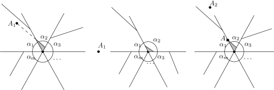
Figure 9: Reduce the number of pieces containing the same point. The two figures on the left show the modification we perform if none of the star centers are on an extension of the shared boundary with the other star center. The right figure shows the case when both star centers lie on an extension of the shared segment. The gray triangle marks the area we transfer from $Q_{2}$ to $Q_{1}$.

We now modify the partition to remove all sight lines that contain some star center in their interior. Let $\ell=A_{0}C$ be a sight line that contains $A_{1},A_{2},\dots,A_{m}$ in its interior. We first choose a sequence of points $C_{1},C_{2},\dots,C_{m}$ along the next edge of $Q_{0}$; see Figure 10. We then give the quadrilateral $A_{i}A_{i+1}C_{i+1}C_{i}$ to piece $Q_{i}$ for all $i\in\{1,2,\dots,m-1\}$. Finally we give $A_{m}CC_{m}$ to $Q_{m}$. This modification removes all star centers from the interior of one sight line while no newly created sight line contains a star center in its interior. It is easy to check that this modification of the partition does not make four pieces meet.

Figure 10: Redistributing pieces to remove a sight line that contains star centers in its interior.

∎

The main tool in this section is restricted coordinate maximum partitions defined in Section 2. The following lemma captures one of our key combinatorial results on a star center in a restricted coordinate maximum partition from Lemma 4. Intuitively, if one moves a star center $A_{k}$ of an optimal star partition in the direction $d$ as far as possible without moving other star centers (but possibly changing what region of $P$ each piece contains), then there are only a few reasons to get stuck.

Lemma 7.

Consider the restricted coordinate maximum optimal star partition consisting of simple polygons $\mathcal{Q}=\{Q_{1},\ldots,Q_{k}\}$ along $d$, within $F$, and with fixed star centers $A_{1},\ldots,A_{k-1}$ (so that only the coordinates of the last center $A_{k}$ have been maximized). Suppose that no four pieces meet in the same point and no star center is in the interior of any sight line. Then $A_{k}$ lies on the intersection of two non-parallel segments of the following types:

• an edge of $F$,

• an important sight line of $Q_{k}$, not containing any other star center, which is

  • an extension of an edge of $P$, or

  • on the extension of a diagonal of $P$ that connects two concave corners, or

  • an extension of a tripod leg (see Section 2), and no star center is in the interior of the pseudo-triangle of this tripod.

Proof.

We can choose $A_{k}$ freely inside $\ker(Q_{k})\cap F$ while all the pieces remain the same. By coordinate maximization, $A_{k}$ must be a corner of $\ker(Q_{k})\cap F$. Let $\mathcal{S}$ denote the set of edges $e$ of $Q_{k}$ such that $A_{k}$ is on the extension of $e$. Let $\mathcal{S^{\prime}}$ denote the set of edges of $F$ that $A_{k}$ lies on. Since all edges of $\ker(Q_{k})$ come from extensions of edges of $Q_{k}$, there must be two non-parallel segments in $\mathcal{S}\cup\mathcal{S^{\prime}}$.

We call a segment in $\mathcal{S}$ good if it is collinear to a segment that is of the described types in the lemma statement; otherwise, we call it bad. In the remainder of the proof, we modify the partition $\mathcal{Q}$ while not moving any star centers and never creating any new important sight lines of $Q_{k}$, which means that the two good segments we find at last are also good segment of the initial star partition $\mathcal{Q}$. At the same time, we decrease the number of bad segments in $\mathcal{S}$ until all segments in $\mathcal{S}$ are good. In the end, either $A_{k}$ satisfies the lemma, or else we cannot find two non-parallel segments in $\mathcal{S}\cup\mathcal{S}^{\prime}$, which would mean that $A_{k}$ is not at a corner of $\ker(Q_{k})\cap F$ therefore contradicting that $A_{k}$ is optimal with respect to coordinate maximization.

In the remainder of the proof, all star centers and corners of $P$ on $\partial Q_{k}$ are considered as corners of $Q_{k}$, so there can be several collinear consecutive segments of $Q_{k}$. First, we consider the case that $A_{k}$ is the endpoint of a bad segment in $\mathcal{S}$.

1. $A_{k}$ is a corner of $P$. Then $A_{k}$ must be a corner of $F$ as $F\subset P$. Hence $A_{k}$ is at two edges of $P$ and the lemma holds.

2. $A_{k}$ is in the interior of an edge of $P$. If $A_{k}$ is a corner of $F$, then the lemma holds. Otherwise, $A_{k}$ is in the interior of an edge of $F$ that is collinear to the boundary of $P$. We can assign an arbitrarily small region around $A_{k}$ to $Q_{k}$ such that $A_{k}$ is not an endpoint of a bad segment anymore; see Figure 11. Since we do not create any new important sight line in $Q_{k}$, we do not introduce any new good segments in $\mathcal{S}$. The only new bad segment we introduce is parallel to the boundary edge of $P$ that $A_{k}$ lies on, which can also be removed from $S$ without breaking the assumption that $S\cup S^{\prime}$ contains two non-parallel segments— since there must be an parallel edge of $F$.

   

   Figure 11: Dealing with the case that $A_{k}\in\partial P$. The gray region marks the region that we give to $Q_{k}$.

3. $A_{k}$ is in the interior of $P$. This can happen when $A_{k}$ is either a convex corner of all pieces touching it, a concave corner of the piece $Q_{k}$, or a concave corner of some other piece. In all cases, we transfer a sufficiently small area around $A_{k}$ to $Q_{k}$ and thereby make $A_{k}$ not be an endpoint of a bad segment; see Figure 12.

   

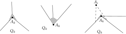
   Figure 12: Dealing with the case that $A_{k}\in\partial Q_{k}$. The gray region marks the region that we give to $Q_{k}$. The first figure shows the case that $A_{k}$ is a convex corner for all pieces; the second shows the case that $A_{k}$ is a concave corner of $Q_{k}$; the third shows the case that $A_{k}$ is a concave corner of other pieces.

In the following $A_{k}$ is not an endpoint of a bad segment in $\mathcal{S}$. Let $e=C_{1}C_{2}$ be a segment in $\mathcal{S}$ and let $C_{2}$ be the farther end of $e$ from $A_{k}$. Let $C_{0}$ be the closest point to $A_{k}$ on $A_{k}C_{1}$ such that $C_{0}C_{1}\subset\partial Q_{k}$ (it might be the case that $C_{0}=C_{1}$). Note that this implies $C_{0}\neq A_{k}$, as $A_{k}$ is not the endpoint of a bad segment in $\mathcal{S}$. Furthermore, let $C_{3}$ be the farthest point from $A_{k}$ in the direction of $C_{2}$ on the extension of $A_{k}C_{2}$ such that $C_{2}C_{3}\subset\partial Q_{k}$ (it might be the case that $C_{3}=C_{2}$). Let $C_{4}$ be the next corner of $C_{3}$ on $\partial Q_{k}$, and let $C_{-1}$ be the previous corner of $C_{0}$ on $\partial Q_{k}$. We again consider multiple cases:

1. Another star center $A_{i}$ is on $A_{k}C_{3}$. According to our assumptions in the lemma statement, no star center is in the interior of a sight line, thus we have $A_{i}=C_{3}$. We can then transfer the triangle $C_{0}C_{3}C_{4}$ from $Q_{k}$ to $Q_{i}$ and the number of bad segments in $\mathcal{S}$ is thereby reduced; see Figure 13.

   

   Figure 13: If the sight line ends at another star center $A_{i}$, we can give the triangle $C_{0}C_{3}C_{4}$ to $Q_{i}$ and reduce $|\mathcal{S}|$.

2. No corner of $P$ is in the interior of the sight line $A_{k}C_{2}$. Or equivalently, $A_{k}C_{2}$ is not an important sight line. In this case we give a sufficiently small triangle $C^{\prime}C_{0}C_{2}$ to $Q_{k}$, where $C^{\prime}$ is sufficiently close to $C_{0}$ on the segment $C_{-1}C_{0}$; see Figure 14. According to Lemma 1, all pieces that are cut by the segment $C^{\prime}C_{2}$ are still star shaped. This way we reduce the size of $\mathcal{S}$ by removing $C_{1}C_{2}$.

   

   Figure 14: No corners of $P$ on $A_{k}C_{2}$.

   In the remainder we can assume that the sight line $A_{k}C_{2}$ is supported by a corner of $P$, i.e., it is an important sight line. Since $A_{k}C_{2}$ is covered by $A_{k}C_{3}$, $A_{k}C_{3}$ is also an important sight line. Let $D$ be the support (Section 2) of $A_{k}C_{3}$. In the remainder we try to remove $DC_{3}$ from $\mathcal{S}$.

3. $C_{3}$ is a convex corner of $P$ and not adjacent to $D$. Note that if $C_{3}$ was a convex corner of $P$ adjacent to $D$, then $A_{k}C_{3}$ would be an extension of an edge $DC_{3}$ of $P$, which is a good segment in $\mathcal{S}$. We can remove a sufficiently small triangle $DC_{3}C^{\prime}$ from $Q_{k}$ for $C^{\prime}$ close enough to $C_{3}$ on segment $C_{3}C_{4}$, and distribute the triangle to the neighboring pieces by extending the edges that end at $DC_{3}$; see Figure 15. Since we do not create concave corners in any pieces they remain star-shaped. The same argument is also applicable if $DC_{3}$ ends in the interior of an edge of $P$ as we can consider the intersection point as a degenerate convex corner of $P$.

   

   Figure 15: The case when the boundary of $Q_{k}$ ends at a convex corner of $P$.

   In the remainder $C_{3}$ is in the interior of $P$.

4. $C_{3}$ is a concave corner of some piece $Q_{i}$. Then $C_{3}$ is a convex corner of $P\setminus Q_{i}$ and we can use a similar modification to remove $DC_{3}$ from $\mathcal{S}$ as in the previous case; see Figure 16.

   

   Figure 16: $C_{3}$ is a concave corner of some piece.

   In the remainder, $C_{3}$ a convex corner of all its adjacent pieces. According to the assumption of the lemma that no four pieces meet at the same point, $C_{3}$ is contained in at most three pieces. Since the angle of $Q_{k}$ at $C_{3}$ is strictly less than $\pi$, there actually must be exactly three pieces containing $C_{3}$. With slight abuse of notation, let $Q_{0}=Q_{k},Q_{1},Q_{2}$ be these three pieces in clockwise order; let $\alpha_{i}$ be the angle of $Q_{i}$ at $C_{3}$; and let $A_{i}$ be the star center of $Q_{i}$.

5. $C_{3}$ is not a tripod point. If an edge at $C_{3}$ is not covered by an important sight line, we can modify the partition and remove $DC_{3}$ from $\mathcal{S}$; see Figure 17. Otherwise, all edges at $C_{3}$ are covered by important sight lines. As $C_{3}$ is not a tripod point, we have that $\alpha_{1}=\pi$ or $\alpha_{2}=\pi$. If $\alpha_{1}=\pi$, let $D^{\prime}$ be the support of $A_{1}C_{3}$. Now $A_{k}C_{3}$ is on the extension of the diagonal $DD^{\prime}$ that connects two concave corners of $P$. If $\alpha_{2}=\pi$, then $C_{3}$ is a convex corner of $P\setminus Q_{2}$ and we can modify the partition similar to case 3.

   

   Figure 17: The case when an edge at $C_{3}$ is not covered by important sight line.

   In the remainder $C_{3}$ is a tripod point. Note that if the tripod associated with $C_{3}$ contains no star center in its pseudo-triangle, then the edge $C_{1}C_{2}$ is a good edge. Hence, the only remaining case is the following.

6. $C_{3}$ is a tripod point and a star center is in the interior of the pseudo-triangle of this tripod. Let $A_{3}$ be the star center inside the pseudo-triangle. The tripod partitions $P$ into three regions $R_{0},R_{1},R_{2}$, where $R_{i}$ is the region containing $A_{i}$. Let $R^{\prime}_{i}$ be the intersection of $R_{i}$ and the pseudo-triangle. First we prove that there exists a segment $XY$ from one leg of the tripod to another leg that contains a star center $A^{\prime}_{3}$ and no star center is in the interior of triangle $C_{3}XY$. Let $R^{\prime}_{j}$ be the region that contains $A_{3}$. Consider the convex hull $\mathcal{C}$ of all corners of this pseudo-triangle and all star centers in $R^{\prime}_{j}$. There exists a corner of $\mathcal{C}$ that is a star center $A^{\prime}_{3}$, as $A_{3}$ lies in the interior of $R^{\prime}_{j}$. Let $\ell$ be an arbitrary tangent of $\mathcal{C}$ at $A^{\prime}_{3}$, and let $XY$ be the subsegment of $\ell$ that is contained in the pseudo-triangle. Whichever region $A_{3}$ lies in, we can modify the partition so that the tripod is broken and $|\mathcal{S}|$ is not increased; see Figure 18. Since the number of possible tripods is finite, we can apply the argument a finite number of times and then either the size of $\mathcal{S}$ is decreased, or $A_{k}C_{3}$ becomes a good segment. ∎

   

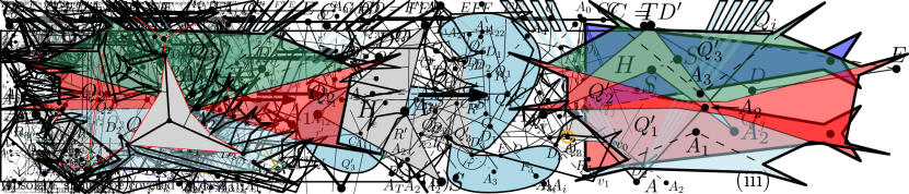
   Figure 18: Three cases of where the star center $A^{\prime}_{3}$ is and how we define the gray triangle to give to $A^{\prime}_{3}$.

3.1 Tripod Trees

We now define what we call the tripod tree—a description of the structure of tripods in an optimal solution (see also Figure 19). Given a star partition, consider the partition that is induced by the tripod legs. Note that this partition is simply the star partition but with some pieces having been merged. We construct a bipartite graph $G=(X\cup Y,E)$ as follows:

• We add a vertex to $X$ for each face of the partition induced by the legs.

• We add a vertex to $Y$ for each tripod.

• We add an edge $\{x,y\}$ to $E$ if and only if a tripod leg of $y$ forms part of the boundary of $x$.

Observation 8.

Given a star partition, the tripod tree graph $G$ is indeed a tree.

Proof.

If the tripods are considered degenerate pieces of the partition, then $G$ corresponds to the dual graph of the partition induced by the legs. Thus, $G$ is connected. Furthermore, note that every tripod cuts the polygon $P$ into three disconnected pieces, so the corresponding vertex in $Y$ is a cut vertex, which implies that $G$ is a tree. ∎

We choose the root of the tripod tree to be the face that contains the first edge of $P$, merely for consistency. For every tripod $\mathcal{T}$ formed by pieces $Q_{i},Q_{j},Q_{k}$ where $Q_{i}$ is contained in the parent face of $\mathcal{T}$, we call the star center $A_{i}$ of $Q_{i}$ the parent star center of $\mathcal{T}$ and the star centers $A_{j},A_{k}$ of $Q_{j},Q_{k}$ are both called child star centers of $\mathcal{T}$. Note that we can directly identify the parent star center of a tripod without the full tripod tree.

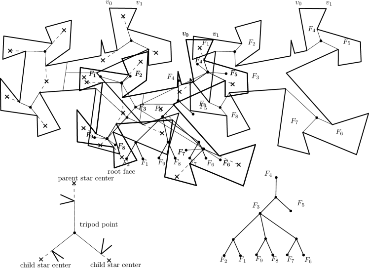
Figure 19: Illustration for a tripod tree. A cross represents a star center, a solid circle represents a tripod point. Top-left figure shows a star partition. Top-right figure shows the faces splits by all the tripod legs. Bottom-left figure shows the orientation of a tripod. Bottom-right figure shows the rooted tripod tree induced by this star partition.

Fake tripod.

In a star partition $\mathcal{Q}$, a fake tripod $\mathcal{T}^{\prime}$ with tripod point $C$ is defined by two star centers $A_{1},A_{2}$ of pieces $Q_{1},Q_{2}$ and three concave corners $D_{1},D_{2},D_{3}$ of $P$ if the following properties hold.

• $A_{i}C$ is an important sight line of $Q_{i}$ with support $D_{i}$, for each $i\in\{1,2\}$.

• $A_{i}C\subset\bigcup_{Q\in\mathcal{Q}}\partial Q$ for each $i\in\{1,2,3\}$.

• The three angles $D_{1}CD_{2},D_{2}CD_{3},D_{3}CD_{1}$ are strictly convex.

• Let $F_{1},F_{2},F_{3}$ be the three connected components of $P$ cut by $D_{1}C\cup D_{2}C\cup D_{3}C$, where $A_{1}\in F_{1},A_{2}\in F_{2}$, $F_{3}$ contains the first edge of $P$. $D_{3}$ is a concave corner in $F_{3}$. The union $Q_{1}\cup Q_{2}\cup F_{3}$ contains a (sufficiently small) disk at $C$.

Similarly as for tripods, the three segments $D_{1}C,D_{2}C,D_{3}C$ are called the legs of $\mathcal{T}^{\prime}$, $A_{1},A_{2}$ are called child star centers of $\mathcal{T}^{\prime}$, and the polygon bounded by the shortest paths between pairs of supports $D_{1},D_{2},D_{3}$ is called the pseudo-triangle of $\mathcal{T}^{\prime}$.

Note that for every tripod $\mathcal{T}$, there is exactly one fake tripod $\mathcal{T}^{\prime}$ with the same tripod point and legs, which is defined by its supports and the two child star centers of $\mathcal{T}$. We say $\mathcal{T}^{\prime}$ is the associated fake tripod of $\mathcal{T}$.

Figure 20: Left: a fake tripod defined by star-centers $A_{1},A_{2}$ and supports $D_{1},D_{2},D_{3}$. Note that $A_{3}^{\prime}$ is not on the extension of $CD_{3}$. Right: a tripod and its associated fake tripod, since there exists the third star-center $A_{3}$ on the extension of $CD_{3}$.

Remark 9.

We introduce the concept of fake tripods (see also Figure 20) to facilitate our algorithm. The final algorithm will simulate the construction process (described in the following Section 3.2) and get a full partition in the end. We can not easily decide whether a (real) tripod exists unless we find both its two child star centers and its parent star center. Algorithmically, it is much easier to construct the fake tripods in a bottom-up fashion just using the two child star centers, without knowledge of where (or if) a potential third parent star-center might exist.

3.2 Construction Process

We now describe an iterative construction process of star centers and fake tripods. We will show that there exists an optimal star partition for which all star centers can be constructed using this process in linear steps. The construction process is with respect to a star partition $\mathcal{Q}$ and is a process to “mark” star centers and fake tripods of $\mathcal{Q}$ as “constructable”. Formally, we call a star center or a fake tripod constructable (with respect to $\mathcal{Q}$) if it can be marked by the following process. At each step in the process, we can do one of the following operations:

• Mark a star center $A_{k}$ at the intersection of two non-parallel segments of the following types:

  1. An edge of $P$;

  2. An edge of the pseudo-triangle of a marked fake tripod;

  3. An important sight line of a piece $Q_{k}$, which is on the extension of

     • an edge of $P$;

     • a diagonal of $P$ that connects two concave corners of $P$;

     • a tripod leg of a tripod $\mathcal{T}$ whose extension contains the parent star center of $\mathcal{T}$, while the corresponding fake tripod $\mathcal{T}^{\prime}$ of $\mathcal{T}$ is marked.

• Mark a fake tripod $\mathcal{T}^{\prime}$ defined by two marked star centers $A_{i},A_{j}$ and three concave corners $D_{i},D_{j},D_{k}$ of $P$. Additionally, there must be no star center (marked or unmarked) in the interior of the pseudo-triangle of $\mathcal{T}^{\prime}$.

An optimal star partition $\mathcal{Q}$ is called constructable if all the star centers in $\mathcal{Q}$ is constructable with respect to $\mathcal{Q}$.

Now comes the major structural result in this section, which gives us a combinatorial way to describe some optimal star partition.

Theorem 10 (Construction of optimal star partition).

There exists a constructable optimal star partition $\mathcal{Q}$.

Remark 11.

We can also define a similar construction process if we replace tripod by fake tripod. Actually the two definition would agree on whether a partition is constructable or not. When a fake tripod is used to construct a star center, it turns to a tripod; otherwise, we do not need to mark that fake tripod.

Instead of proving this theorem, we prove the following stronger lemma, which allows us to extend a “partially constructable” optimal solution into a constructable one. This lemma also helps us to prove the correctness of the greedy choice (see Section 5.2.1) used when choosing tripods, which is the main technique to improve the running time of our dynamic programming algorithm into polynomial time in Section 5.

Lemma 12.

Let $\mathcal{Q}$ be an optimal star partition of $P$ such that some star centers $A_{1},A_{2},\dots,A_{k}$ and some fake tripods $\mathcal{T}^{\prime}_{1},\mathcal{T}^{\prime}_{2},\dots,\mathcal{T}^{\prime}_{l}$ are constructable with respect to $\mathcal{Q}$. Suppose there exists a star center in $\mathcal{Q}$ which is not constructable with respect to $\mathcal{Q}$, then there exists an optimal solution $\mathcal{Q}^{\prime}$ containing $A_{1},A_{2},\dots,A_{k},A_{k+1}$ as star centers and $\mathcal{T}^{\prime}_{1},\mathcal{T}^{\prime}_{2},\dots,\mathcal{T}^{\prime}_{l}$ as tripods, such that $A_{1},A_{2},\dots,A_{k},A_{k+1}$ and $\mathcal{T}^{\prime}_{1},\mathcal{T}^{\prime}_{2},\dots,\mathcal{T}^{\prime}_{l}$ are constructable.

Proof.

A star center is called missing if it’s not constructable with respect to $\mathcal{Q}$. Consider the construction process of all the constructable star centers and fake tripods. Throughout the construction process we maintain what we call the feasible region, which initially consists of the whole polygon $P$. When a fake tripod with center $C$ is marked by two marked star centers $A_{1},A_{2}$ and three concave corners $D_{1},D_{2},D_{3}$, we partition the polygon into three parts (according to the legs of the fake tripod) and remove the pseudo-triangle of this fake tripod from the feasible region. Moreover, we add two segments $A_{1}D_{1},A_{2}D_{2}$ as an incision into the boundary of both the polygon and the feasible region. See Figure 21 for illustration. This way, we fix the two important sight lines $A_{1}C$ and $A_{2}C$, and make sure that no star centers are in the interior of the pseudo-triangle of this tripod in the following steps. When a star center $A_{i}$ is marked by an important sight line $\ell$ of $Q_{i}$, we also add $\ell$ as an incision into the boundary of both the polygon and the feasible region.

Figure 21: The figure shows the feasible region and the partition of the polygon where some star centers and fake tripods are marked. Red lines mark the boundary of feasible region, and some of them are merely incisions. The gray region marks the pseudo-triangle of the marked fake tripod, which is not a part of the feasible region, but the feasible region covers everything else. Thick black lines represent how we partition the polygon into three parts. Each black circle represents a marked star center or a marked fake tripod.

Since the constructable fake tripods partition the polygon into disconnected pieces, we can consider the construction process within each connected part independently. Let $P^{\prime}$ be such a connected part for which at least one star center is not constructable. If there are multiple choices, we will choose one later. Let $F$ be the feasible region inside $P^{\prime}$. We now restrict our polygon to be $P^{\prime}$.

We perform a restricted coordinate maximization along an arbitrary direction $d$ as described in Lemma 4 within $F$ and with all the contructable star centers fixed. By optimality, for each missing star center, the partition is also restricted coordinate-maximal along $d$, within $F$ and with all the other star centers fixed. Applying Lemma 7, we know that all the missing star centers lie on the intersection of two non-parallel segments of certain types. We call these segments the crucial segments. The goal of the following discussion is to mark a new star center using crucial segments. Therefore, we enumerate the types of crucial segments and check whether they are allowed in the construction process.

Case 1: A crucial segment is an edge of $F$. Every edge of $F$ is an edge of $P$, or a segment on the boundary of a pseudo-triangle, or an important sight line that was used to construct a constructable star center. Note that all segments on the boundary of a pseudo-triangle must be diagonals that connect two concave corners of $P$. Hence, all the edges of $F$ can be used to construct new star centers.

Case 2: A crucial segment is an important sight line in $P^{\prime}$. Note that all corners of $P^{\prime}$ are either corners of $P$, or constructable star centers, or tripod points of a constructable fake tripod. Each tripod point is a convex corner in any connected part separated by the tripod legs, hence they can only induce convex corners of $P^{\prime}$. Consequently, a concave corner of $P^{\prime}$ is either a concave corner of $P$ or a constructable star center. According to Lemma 7, no other star center lies on a crucial segment, so the crucial segment that the star center lies on must be supported by a concave corner of $P$, which implies that the crucial segment is also an important sight line when we consider the full polygon $P$. If the crucial segment ends at a concave corner of $P^{\prime}$, it must end at a concave corner of $P$, as crucial segments are not allowed to contain another star center. Hence, it is contained in an extension of a diagonal of $P$ that connects two concave corners of $P$.

Thus, a crucial segment cannot be used to mark star centers only if it is an extension of a tripod leg, and either the corresponding fake tripod is not constructable, or the star center is not in the parent face of this tripod.

We now consider the tripod tree of $\mathcal{Q}$. We call a tripod illegal if there exists a missing star center in its child face. Otherwise, we call a tripod legal. Then, a star center is missing only if one of its crucial segments end at the tripod point of an illegal tripod. As there exists a missing star center, there also exists an illegal tripod.

Let $\mathcal{T}$ be an illegal tripod such that all tripods contained in the subtree rooted at $\mathcal{T}$ are legal. Note that there exists a missing star center in at least one of its child faces. Hence, all star centers in the two child faces of $\mathcal{T}$, except for the child star centers of $\mathcal{T}$, are constructable. Let $A$ be a missing child star center of $\mathcal{T}$. We choose $P^{\prime}$ to be the connected component containing $A$.

We perform a restricted coordinate maximization on $A$, where the polygon we are going to partition is the part of $P^{\prime}$ cut by $\mathcal{T}$ that $A$ lies in, and the feasible region is $F$ excluding the pseudo-triangle of $\mathcal{T}$ restricted to the current polygon. We choose $d$ to be the direction perpendicular to the important sight line that $A$ ends at the tripod point of $\mathcal{T}$ and points to the unsupported side. The choice of direction $d$ makes it impossible that the new star center $A^{\prime}$ lies on the same important sight lines from $\mathcal{T}$, unless it is also on other two non-parallel crucial segments.

By a similar analysis of the types of crucial segments that the new star center $A^{\prime}$ lies on, $A^{\prime}$ cannot be marked in the next step only if it is a child star center of an illegal tripod contained in $P^{\prime}$, and we resolve this case recursively; see Figure 22. Since the subpolygon cut by the new illegal tripod has strictly fewer corners, this recursion will finish in finite steps. Eventually, we can find an optimal partition in which one more star center $A^{\prime}$ is constructable by the intersection of two non-parallel crucial segments. ∎

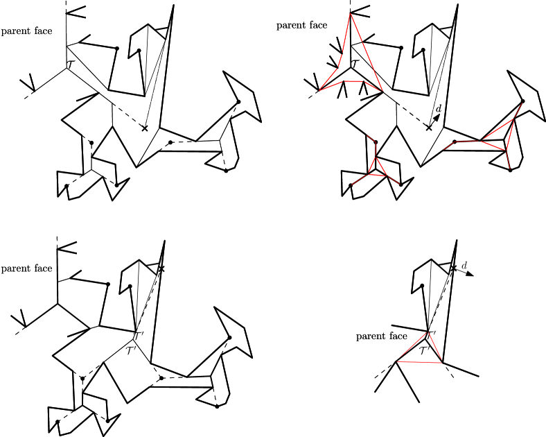
Figure 22: Illustration for the proof of Theorem 10. A constructable star center is represented by a solid circle, and the missing star center is represented by a cross. Red segments mark the boundary of the feasible region, and thick black segments mark how we partition the polygon into parts. The top-left figure shows the partition $\mathcal{Q}$, and the top-right figure shows the restricted coordinate maximization problem used in the proof. The bottom-left figure shows the restricted coordinate maximization partition of this problem. The old illegal tripod $\mathcal{T}$ is no longer a tripod, but we get a new illegal tripod $\mathcal{T}^{\prime}$, which will be resolved recursively. The bottom-right figure shows this new subproblem that we get. Since the number of vertices on the boundary are strictly fewer, the recursion will eventually terminate.

The following lemma gives us another useful property of constructable optimal star partition, which will be used to design our dynamic programming algorithm in Section 5.

Lemma 13.

Let $\mathcal{Q}$ be a star partition of $P$. If a star center $A_{k}$ is constructable with respect to $\mathcal{Q}$, then a corner of $P$ appears on the boundary of the piece $Q_{k}$.

Proof.

We consider the different cases in the construction process which can lead to the star center $A_{k}$ being marked. If $A_{k}$ is marked by an important sight line $\ell$ of $Q_{k}$, then the support $D^{\prime}$ of $\ell$ is a corner of $P$ in $Q_{k}$, and the lemma holds. If $A_{k}$ is at the intersection of two edges of $P$, $A_{k}$ must be a corner of $P$. If $A_{k}$ is at the intersection of an edge of $P$ and an edge of a pseudo-triangle, $A_{k}$ must be a corner of $P$, as the intersection of the pseudo-triangle and the boundary of $P$ is just a set of concave corners of $P$. If $A_{k}$ is at the intersection of two non-parallel edges from the same pseudo-triangle, $A_{k}$ must be a corner of this pseudo-triangle, and it therefore is also a concave corner of $P$. If $A_{k}$ is at the intersection of two non-parallel edges from different pseudo-triangles, according to Lemma 2, $A_{k}$ must be a corner of one pseudo-triangle, therefore $A_{k}$ is also a corner of $P$. ∎

From this lemma, we directly have the following corollary, which will be used to prove some combinatorial properties of an optimal partition in Section 5.

Corollary 14.

For any constructable optimal star partition $\mathcal{Q}=Q_{1},\dots,Q_{k}$, we have $Q_{i}\cap\partial P\neq\emptyset$, that is every star piece touches the boundary of $P$.

4 Properties of Area Maximum Partitions

The objective of this section is to compute a set of polynomially many points that contains all the Steiner points for some optimal solutions, given all the star centers of an arbitrary optimal solution.

Consider a polygon $P$, a sequence of points $\mathcal{A}=(A_{1},\ldots,A_{k})$, and a star partition $\mathcal{Q}=(Q_{1},\ldots,Q_{k})$ of $P$ where $A_{j}$ is a star center of $Q_{j}$. Recall that $\mathcal{Q}$ is called area maximum with respect to $\mathcal{A}$ if the vector of areas $a(\mathcal{Q})=\langle a(Q_{1}),\ldots,a(Q_{k})\rangle$ is maximum in lexicographic order among all partitions of $P$ with star centers $\mathcal{A}$. In Appendix A we argue that this notion of area maximum partitions is well-defined. Note that in the definition of area maximum partitions, the positions of the star centers are fixed. In this section we prove some properties of area maximum partitions, in particular that all corners of pieces (i.e. Steiner points) are in “nice” spots.

Recall that a sight line of a piece $Q_{i}$ is a segment of the form $r=A_{i}C$, where $A_{i}$ is the star center of $Q_{i}$ and $C$ is a corner of $Q_{i}$. Here, the point $C$ is called the end of $r$.

Lemma 15.

Consider an optimal area maximum partition $\mathcal{Q}$ with a given set of star centers $\mathcal{A}$. For any two pieces $Q_{1},Q_{2}\in\mathcal{Q}$, let $\gamma\coloneqq\partial Q_{1}\cap\partial Q_{2}$ be their shared boundary. Then $\gamma$ is

• empty, or

• a single point, or

• a single line segment contained in a sight line of $Q_{1}$ or $Q_{2}$, or

• two adjacent line segments, each contained in a sight line of $Q_{1}$ or $Q_{2}$.

Figure 23: Situations in the proof of Lemma 15. Left: If $\gamma$ is not connected, $F$ must contain a third piece which can be subsumed by $Q_{1}$ and $Q_{2}$, which is a contradiction. Middle: When $S$ and $T$ are convex, we have $\gamma=SA_{2}\cup A_{2}T$. Right: When $S$ is concave, we have $\gamma=SS^{\prime}\cup S^{\prime}T$.

Proof.

We first prove that $\gamma$ is connected. Otherwise, there exist points $G_{1},G_{2}\in\gamma$ which are not connected by $\gamma$; see Figure 23 (left). Let $A_{i}\in\mathcal{A}$ be the star center of $Q_{i}$. Since $G_{1}$ and $G_{2}$ are not connected by $\gamma$, the quadrilateral $F=A_{1}G_{2}A_{2}G_{2}$ is not contained in $Q_{1}\cup Q_{2}$, but the boundary $\partial F$ is contained. Hence, $F$ contains a third piece from $\mathcal{Q}$. However, the quadrilateral $F$ can be completely assigned to $Q_{1}$ and $Q_{2}$ (possibly after being split in two), so the partition $\mathcal{Q}$ was not optimal, which is a contradiction. Hence, $\gamma$ is connected.

Let $S$ and $T$ be the endpoints of $\gamma$. If $S=T$, the shared boundary is a single point which must be a corner of at least one of the two pieces $Q_{1},Q_{2}$, since otherwise their shared boundary would be longer. Hence, $\gamma$ is contained in a sight line in that case.

Otherwise, let us traverse $\gamma$ from $S$ to $T$; see Figure 23 (middle and right). Since $Q_{1}$ and $Q_{2}$ are star-shaped, we move around $A_{1}$ in a monotone way, either clockwise or counterclockwise, and we move in the opposite direction around $A_{2}$. Hence, $\gamma$ is contained in the quadrilateral $H=A_{1}SA_{2}T$. Assume without loss of generality that $A_{1}$ had higher priority than $A_{2}$ when we maximized the areas of the pieces in $\mathcal{Q}$.

If $S$ and $T$ are both convex corners of $H$, then all of $H$ can be seen from $A_{1}$, so we can assign the quadrilateral $H$ to $Q_{1}$. Then $\gamma$ is a continuous part of $SA_{2}\cup A_{2}T$ with $A_{2}\in\gamma$, so $\gamma$ is contained in two sight lines of $Q_{2}$.

Otherwise, assume without loss of generality that $S$ is concave and $T$ is convex. Let $S^{\prime}$ be the intersection between the line containing the segment $A_{1}S$ and the segment $A_{2}T$. Then we maximize the area of $Q_{1}$ by assigning the triangle $A_{1}S^{\prime}T$ to $Q_{1}$ and the rest of $H$ (which is the triangle $A_{2}SS^{\prime}$) to $Q_{2}$. Hence, we have that $\gamma$ is a continuous part of $SS^{\prime}\cup S^{\prime}T$ with $S^{\prime}\in\gamma$, so $\gamma$ is contained in sight lines of $Q_{1}$ and $Q_{2}$, respectively. Note that it may happen that $S^{\prime}=T$, so that one of these segments is degenerate. ∎

We say that a point $B$ is supporting a sight line $r=AC$ from a star center $A$ if $B\in r\setminus\{A\}$. The following lemma characterizes all edges of pieces of an area maximum partition, using Lemma 15.

Lemma 16.

Consider a piece $Q$ with star center $A$ of an optimal area maximum partition. Let $r=AC$ be a sight line of $Q$ which contains an edge on the boundary of $Q$. Then $r$ is of one of the following types:

1. $r$ is supported by a corner of $P$,

2. $r$ is supported by a star center of another piece, or

3. $C$ is the end of two non-parallel sight lines of type (i) in other pieces.

Proof.

Suppose that a sight line $r=AC$ is supported by no corner of $P$ and no star center of another piece. We will prove that the end $C$ must be the end of two sight lines of type (i) of other pieces. We consider multiple cases.

Figure 24: Situations in the proof of Lemma 16. In Case 1.1 or Case 1.2, we can increase the area of $Q$ or $Q_{1},Q_{2},Q_{3}$ by rotating $r$ clockwise or counterclockwise, respectively.

Case 1: $C$ is an interior point of another sight line or an edge of $P$. Let us denote this sight line or edge by $e$; see Figure 24. Let $f=DC$ be the edge of $Q$ contained in $r$. Assume without loss of generality that $r$ is horizontal with the end $C$ to the right and that the interior of $Q$ is above $f$. Then some other pieces $Q_{1},\ldots,Q_{i}$ are below $f$. Recall that in an area maximum partition, we maximize the vector of areas in a specific lexicographic order; in other words, each piece has a distinct priority when maximizing the areas. In both of the following cases we obtain a contradiction.

Case 1.1: $Q$ has higher priority than all of $Q_{1},\ldots,Q_{i}$. In this case, we can expand $Q$ a bit by rotating $r$ a bit clockwise around $A$, thus “stealing” some area from the pieces $Q_{1},\ldots,Q_{i}$ and increasing the area vector with respect to the lexicographic order.

Case 1.2: One of the pieces $Q_{1},\ldots,Q_{i}$ has higher priority than $Q$. In this case, we can rotate $r$ a bit counterclockwise, thus expanding the pieces $Q_{1},\ldots,Q_{i}$ and increasing the area vector. We conclude that $C$ is not an interior point of another sight line or an edge of $P$.

Case 2: $C$ is the end of one or more sight lines of other pieces. First, note that according to Lemma 15 all boundaries ending at $C$ are sight lines. Let the sight lines that share the end $C$ be $r_{1},\ldots,r_{i}$ in counterclockwise order (one of these is $r$), and let the associated set of pieces and star centers be $\mathcal{Q}=\{Q_{1},\ldots,Q_{i}\}$ and $A_{1},\ldots,A_{i}$, respectively. We first observe that we must have $i\geq 3$: Clearly $i\geq 2$, so consider the case $i=2$. If the two sight lines $r_{1}$ and $r_{2}$ are not parallel, then $C$ is a concave corner of one of them that causes the piece to not be star-shaped. If the two sight lines are parallel, then $C$ is not a corner of the pieces, so $r_{1}$ and $r_{2}$ are not (complete) sight lines of the pieces. Hence, $i\geq 3$.

Assume without loss of generality that the interior of each $Q_{j}$ is to the left of $r_{j}$. This has the consequence that if $r_{j}$ is supported by a corner of $P$, then the two incident edges are to the right of $r_{j}$ and likewise, if $r_{j}$ is supported by a star center, then the interior of the associated piece is also to the right. We can furthermore without loss of generality assume that $Q_{1}$ has highest priority among pieces in $\mathcal{Q}$ when maximizing the areas. Suppose towards a contradiction that at most one of the sight lines $r_{1},\ldots,r_{i}$ is supported by a corner of $P$—note that otherwise $r$ is a sight line of type (iii). Let $\mathcal{R}$ be the set of pieces $R$ for which $R\notin\mathcal{Q}$ but $\partial R\cap r_{j}\neq\emptyset$ for some $j\in\{1,\dots,i\}$.

Case 2.1: $Q_{1}$ has higher priority than all pieces in $\mathcal{R}$. Without loss of generality, we assume that $r_{1}$ is horizontal with $C$ to the right.

Figure 25: Case 2.1.1 in the proof of Lemma 16.

Case 2.1.1: The sight line $r_{1}$ is not supported by a corner of $P$. If $r_{1}$ is supported by a star center, then let $A_{R}$ be the star center on $r_{1}$ closest to $C$ and let $R\in\mathcal{R}$ be the piece with center $A_{R}$; see Figure 25—note here that $C$ is not a star center as otherwise $r$ is of type (ii). If $r_{1}$ is not supported by a star center, let $R=Q_{1}$ and thus $A_{R}=A_{1}$. Let $D_{1}$ and $D_{2}$ be points on sight lines among $r_{2},\ldots,r_{i}$ such that the interior of the quadrilateral $\Delta=A_{1}A_{R}D_{1}D_{2}$ contains $C$ but no star center or corner of $P$ and intersects only pieces in $\mathcal{Q}\cup\mathcal{R}$; such points $D_{1}$ and $D_{2}$ exist since, otherwise, a piece among $Q_{1},\ldots,Q_{i}$ would have a concave corner at $C$ (and the piece would not be star-shaped) or $C$ would be an interior point on one of the sight lines $r_{1},\ldots,r_{i}$. We split $\Delta$ by the line containing $r_{1}$ and assign the part to the left to $Q_{1}$ and the part to the right to $R$. The area vector is thereby increased, which is a contradiction.

Figure 26: Case 2.1.2 in the proof of Lemma 16. Top: We change the partition so that no star center is supporting a sight line from the right. Bottom: When no star center supports a sight line from the right, we can move $C$ to the right, thus expanding $Q_{1}$.

Case 2.1.2: The sight line $r_{1}$ is supported by a corner of $P$. We show how to extend $r_{1}$ so that $C$ moves to the right; see Figure 26. All other sight lines $r_{l}$ are then adjusted by rotating and extending/contracting appropriately, which makes $Q_{1}$ grow, thus increasing the area vector and resulting in a contradiction. This is only possible—recall that $r_{1}$ is the only sight line supported by a corner of $P$—if no sight line $r_{l}$ is supported by a star center with the associated piece meeting $r_{l}$ from the right. Suppose that there is such a star center $A_{U}$ supporting a sight line $r_{l}$ from the right, and assume that $A_{U}$ is the star center on $r_{l}$ closest to $C$. Note that we must have $l\neq 1$, since $r_{1}$ is horizontal. Let $B$ be the corner of $Q_{l}$ after $C$ in counterclockwise order. We then assign the triangle $A_{U}CB$ to the piece $U$ with center $A_{U}$. We do this modification for all sight lines supported by a star center from the right. It is then possible to extend $r_{1}$ so that $C$ moves to the right and $Q_{1}$ grows, which is a contradiction.

Figure 27: Case 2.2 in the proof of Lemma 16. It is impossible that the piece $T$ touches $r_{j}$ only in a single point $S$, since we can then expand $T$ by adding the triangle $A_{T}SS^{\prime}$.

Case 2.2: The piece $T\in\mathcal{R}$ with maximum priority has higher priority than $Q_{1}$. Let $A_{T}$ be the star center of $T$ and let $r_{j}$ be the sight line touching $T$. Without loss of generality, we can assume that $r_{j}$ is horizontal with $C$ to the right. Then $Q_{j}$ is above $r_{j}$ and $T$ must be below $r_{j}$. Suppose first that $T\cap r_{j}$ is a single point $S$; see Figure 27. This is impossible, because we can choose another point $S^{\prime}\in r_{j}$ and assign the triangle $A_{T}SS^{\prime}$ to $T$ and thus increase the area vector.

Figure 28: Cases 2.2.1 and 2.2.2 in the proof of Lemma 16.

Case 2.2.1: No sight line is supported by a corner of $P$. Let $r_{m}$ be a sight line which is not identical to or parallel with $r_{j}$; see Figure 28 (top). In a way similar to Case 2.1.2, we will extend or contract $r_{m}$ so that $C$ moves upwards: if $r_{m}$ is in the half-plane below $r_{j}$, we will extend and otherwise, we contract. This is only possible if no sight line $r_{l}$ is supported by a star center with the associated piece meeting $r_{l}$ from above. We can eliminate such star centers as described in Case 2.1.2. It is then possible to extend or contract $r_{m}$ so that $C$ moves upwards and $T$ grows, which is a contradiction.

Case 2.2.2: One sight line $r_{m}$ is supported by a corner of $P$. If the incident edges of $P$ are below $r_{m}$, we can do as in Case 2.2.1, so suppose the edges are above $r_{m}$. Furthermore, if $r_{m}$ is not horizontal, we can extend or contract $r_{m}$ so that $C$ moves up and $T$ grows as in Case 2.2.1, which is a contradiction; see Figure 28 (bottom). We are left with the case that $r_{m}=A_{m}C$ is horizontal with $C$ to the left. Since at least three sight lines meet at $C$, we can consider a sight line $r_{l}$ which is not parallel to $r_{j}$ and $r_{m}$. We can then do as in Case 1, where the union $r_{j}\cup r_{m}$ plays the role of the segment $e$ and we either expand $Q_{l}$ or one of the pieces meeting $r_{l}$ from the right, whichever has larger priority.∎

Figure 29: Examples of the different sight line types of Lemma 16 and different Steiner points these can give rise to, as characterized by Corollary 17. The sight lines $A_{4}Z_{1}$ and $A_{5}Z_{1}$ are of type (i) (supported by a corner of $P$), meeting in point $Z_{1}$. The sight line $A_{2}Z_{2}$ is of type (ii) (supported by star center $A_{3}$). The sight line $A_{1}Z_{1}$ is of type (iii) (ending in the common endpoint of two sight lines of type (i)). We note that $Z_{2}$ here is a Steiner point arising from a sight line of type (ii) ending on a sight line of type (iii). There are five star centers and two corners of $P$ involved in the definition of Steiner point $Z_{2}$, which turns out to be the worst case. In our algorithm, we will have $O(n^{6})$ potential star centers, making for a total of $O(n^{32})$ potential such Steiner points.

See Figure 29 for an example of the different types of sight lines and Steiner points (i.e. corners of the star pieces) needed in the partition. The following corollary, which characterizes all required Steiner points, is immediate from Lemmas 15 and 16; indeed, each Steiner point must be on the beginning or end of a sight line.

Corollary 17.

In an area maximum partition, each Steiner point is of one of the following types:

1. The end of a sight line of type (i) or (ii) on an edge of $P$,

2. The end of a sight line of type (i) or (ii) on a sight line of type (i)–(iii),

3. The common end of two sight lines of type (i).

4. A star center.

5 Algorithm

In this section we present our polynomial time algorithm to find a minimum star partition of a polygon. We restate our main Section 1 below, that we prove in this section.

*

Remark 18.

Although $O(n^{107})$ is polynomial time, it is not exactly efficient. Since our main result is that the problem is in P (while previously it was not clear whether the problem was even in NP), we have not tried optimizing the running time. We believe that it should not be particularly difficult to significantly improve the exponent from $107$ to something like $\approx 50$ by a more refined analysis. For instance, using a smaller set of potential Steiner points would lead to a smaller state-space of the dynamic program (see Appendix B). Our aim here is to give the simplest possible description of an algorithm with polynomial running time. Our techniques alone might not be sufficient to bring down the exponent to, say, a single digit. We leave it as an open question to optimize the running time as far as possible, or conversely provide fine-grained lower bounds.

Overview.

We begin with a brief overview of our algorithm (see also the technical overview in Section 1.2). There are two main challenges to overcome when designing a minimum star partition algorithm:

• First, even if we are given a set of potential Steiner points, it is not clear how to construct an optimal star-partition.

• Second, we need a way to find these potential Steiner points.

For the first challenge, we devise a dynamic programming algorithm. For the second, we rely heavily on our structural results in Section 3 together with a “greedy choice” lemma. In fact, in order to find the potential Steiner-points, we need to invoke the dynamic programming algorithm (which assumes that we know all the potential Steiner points already) on many smaller instances in a recursive fashion.

Dynamic program.

We begin by assuming that we know a set $S^{\textsc{(centers)}}$ of potential star centers. In Section 5.1 we show a dynamic programming algorithm to find a partition of the polygon into a minimum number of star-shaped pieces such that the star center of each piece is in $S^{\textsc{(centers)}}$. The algorithm runs in $O(\mathrm{poly}(n,|S^{\textsc{(centers)}}|))$ time. There are a few key properties that we show that allow us to define this dynamic programming algorithm (details can be found in Section 5.1):

• We show that using $S^{\textsc{(centers)}}$ and the corners of $P$, we can find a set of all potential Steiner points (e.g.  internal corners of the star pieces). We do this by invoking our structural lemmas about area maximum partitions from Section 4. There will only be $O(\mathrm{poly}(n,|S^{\textsc{(centers)}}|))$ many of these potential Steiner points to consider.

• We argue that each star piece touches the boundary in some optimal partition (Corollary 14).

• The above observation allows us to define a set of natural separators (see also Figure 30) involving at most two star pieces. For points $B_{1},B_{2}$ on the boundary of $P$, star centers $A_{1},A_{2}\in S^{\textsc{(centers)}}$ and a potential internal corner $Z$ on the shared boundary of the two star pieces, we can define a (“long”) separator $B_{1}$-$A_{1}$-$Z$-$A_{2}$-$B_{2}$. We also consider (“short”) separators of the form $B_{1}$-$A_{1}$-$B_{2}$. These separators allow us to define a sub-region $P^{\prime}$ of $P$ on one side of the separator, that we can recursively solve using a dynamic programming approach.

Finding potential star centers.

Given the above mentioned dynamic programming algorithm, the ultimate challenge is finding some relatively small (i.e. polynomial-sized) set of points $S^{\textsc{(centers)}}$ such that some optimal solution only uses star centers from $S^{\textsc{(centers)}}$. However, this turns out to be quite challenging and we present how we overcome this, together with the full algorithm, in Section 5.2.

A first attempt might be to consider $S^{\textsc{(centers)}}$ to be all the $O(n^{4})$ points on the intersections of pairs of diagonals of the polygon. This turns out to not be sufficient, as can be seen in Figure 1. Indeed, the same figure shows that the star center points can have degree as high as $\Omega(n)$ (in particular, the position of some star centers depend on up to $\Omega(n)$ corners of the input polygon).

Instead, here we use our crucial structural properties of optimal star partitions proven in Section 3. Essentially, we show there that the only non-trivial structure in some extreme optimal partitions must be tripods(see Section 2), e.g., like those in Figures 1, 4 and 6. The tripods must be supported by three corners of the polygon, so there are only $O(n^{3})$ such choices where a tripod can appear. However, the location of the tripod point might depend on other tripods (again, see Figure 1 for a recursive construction capturing this). To overcome this, we need a greedy choice property that allows us to argue that, for each potential tripod, there is only a single arrangement of this tripod we need to care about: the one that is least restricting for one of the involved star centers.

To find this greedy arrangement of the tripod, we need to solve the minimum star partition problem on a subregion of the polygon. For this we can recursively call our algorithm to construct potential star centers for this smaller instance, and then use the dynamic programming algorithm to find the optimal star-partition.

In Section 3, we argue that the tripods of some optimal solution are all oriented in a consistent way. Indeed, recall that each tripod is constructed by its two child star centers and used to construct its parent star center, so only one of the three subpolygons fenced off by the tripod depends on the other two subpolygons. This consistent orientation means that all the tripods can be oriented towards some arbitrary root face (see Figure 5). This is crucial for our algorithm since this allows us to bound the number of subproblems to $O(n^{2})$ (each diagonal of $P$ will define a subproblem on the side not containing this root face, that can be solved first and must not depend on the other side).

5.1 Dynamic Program

In this section we prove the following theorem.

Theorem 19.

Suppose we are given a polygon $P$ with $n$ corners. Suppose also that we know some set $S^{\textsc{(centers)}}$ of potential star centers, such that we are guaranteed that there exists an optimal partition of $P$ into the minimum number of star-shaped pieces where: (i) each star piece’s center is in $S^{\textsc{(centers)}}$, and (ii) each star piece contains a corner of $P$. Then we can find such an optimal solution in $O(\mathrm{poly}(n,|S^{\textsc{(centers)}}|))$ arithmetic operations.

Remark 20.

For our purposes, we will have $|S^{\textsc{(centers)}}|=O(n^{6})$, and the total running time of the dynamic programming algorithm in Theorem 19 will be $O(n^{105})$ under the RAM model.

5.1.1 Defining Other Steiner Points

Suppose we are given a polygon $P$ and a set of potential star centers $S^{\textsc{(centers)}}$, as in the statement of Theorem 19. Using these, we will be able to identify all potential Steiner points needed for our dynamic program. The main idea is to consider an optimal partition that is area-maximum, and use our structural results from Section 4 (in particular Corollary 17, that characterizes all potential Steiner points). We will define the set $S^{\textsc{(internal)}}$ of potential Steiner points to be used as corners of the star-shaped pieces. Moreover, we define a smaller set $S^{\textsc{(border)}}\subseteq(S^{\textsc{(internal)}}\cap\partial P)$ of potential corners of the star pieces that are also on the boundary of $P$.

Lemma 21.

Let $P$ be a polygon and $S^{\textsc{(centers)}}$ a set of points satisfying the premise of Theorem 19. Then we can find sets $S^{\textsc{(border)}}$ and $S^{\textsc{(internal)}}$ of size $\mathrm{poly}(n,|S^{\textsc{(centers)}}|)$ such that some minimum star partition $(Q_{1},Q_{2},\ldots Q_{k})$ of $P$ with corresponding star centers $(A_{1},A_{2},\ldots,A_{k})$ satisfies the following properties:

1. Each piece $Q_{i}$ touches the polygon boundary $\partial P$.

2. All star centers $A_{i}$ are contained in $S^{\textsc{(centers)}}$.

3. All corners of $Q_{i}$ are contained in $S^{\textsc{(internal)}}$.

4. All corners of $Q_{i}$ that are also on the boundary of $P$ are contained in $S^{\textsc{(border)}}$.

Construction of Steiner points.

We use the characterization of area maximum partitions from Section 4 in order to define the sets $S^{\textsc{(border)}}$ and $S^{\textsc{(internal)}}$. Figure 29 shows the “worst case” example where some Steiner point depends on five star centers and two corners of $P$. We begin by constructing the sight line types as in Lemma 16.

• Let $L^{(i)}$ be the set of lines passing through a potential star center in $S^{\textsc{(centers)}}$ and a distinct corner of $P$. Note that $|L^{(i)}|=O(n|S^{\textsc{(centers)}}|)$, and they correspond to sight lines of type (i).

• Similarly, let $L^{(ii)}$ be the set of lines passing through a pair of distinct potential star center in $S^{\textsc{(centers)}}$. Note that $|L^{(i)}|=O(|S^{\textsc{(centers)}}|^{2})$, and they correspond to sight lines of type (ii).

• To define $L^{(iii)}$, we first define $S^{(iii)}$ to be the set of points on the intersection of two non-parallel lines in $L^{(i)}$. Then we define $L^{(iii)}$ to be the lines through a potential star center in $S^{\textsc{(centers)}}$ and a distinct point in $S^{(iii)}$. Note that $|S^{(iii)}|=O(n^{2}|S^{\textsc{(centers)}}|^{2})$, so $|L^{(iii)}|=O(n^{2}|S^{\textsc{(centers)}}|^{3})$, and that these correspond to sight lines of type (iii).

Now we are ready to use these sight lines to construct all necessary Steiner points, specifically, the different types specified in Corollary 17.

• Let $S^{(1)}$ be the intersections of a segment of $P$ and a (non-parallel) line in $(L^{(i)}\cup L^{(ii)})$. Note that $|S^{(1)}|=O(n|S^{\textsc{(centers)}}|^{2})$

• Let $S^{(2)}$ be the intersections of a line in $(L^{(i)}\cup L^{(ii)})$ and a (non-parallel) line in $(L^{(i)}\cup L^{(ii)}\cup L^{(iii)})$. Note that $|S^{(2)}|=O(n^{2}|S^{\textsc{(centers)}}|^{5})$

• Let $S^{(3)}:=S^{(iii)}$ be the intersections of two (non-parallel) lines in $L^{(i)}$. Note that $|S^{(3)}|=O(n^{2}|S^{\textsc{(centers)}}|^{2})$.

Finally, we can, by Corollary 17, define our “small” sets of potential Steiner points to consider:

• $S^{\textsc{(internal)}}=\text{corners}(P)\cup S^{(1)}\cup S^{(2)}\cup S^{(3)}$ for internal corners of star pieces, with $|S^{\textsc{(internal)}}|=O(n^{2}|S^{\textsc{(centers)}}|^{5})$.

• $S^{\textsc{(border)}}=\text{corners}(P)\cup S^{(1)}$ for corners of star pieces also on the boundary $\partial P$, with $|S^{\textsc{(border)}}|=O(n|S^{\textsc{(centers)}}|^{2})$.

We additionally note that $S^{\textsc{(centers)}}\subseteq S^{(2)}\subseteq S^{\textsc{(internal)}}$ (since a point $A\in S^{\textsc{(centers)}}$ will lie on at least two lines in $L^{(i)}$ as $P$ has at least three non-collinear corners). Similarly $(S^{\textsc{(centers)}}\cap\partial P)\subseteq S^{(1)}\subseteq S^{\textsc{(border)}}$.

Proof of Lemma 21.

Consider any minimum star partition $\mathcal{Q}=(Q_{1},Q_{2},\ldots Q_{k})$—with star centers $(A_{1},A_{2},\ldots A_{k})$—of $P$ that satisfies the premise of Theorem 19: that is each star center is in $S^{\textsc{(centers)}}$ and each piece touch the boundary of $P$ at some corner.

We now consider an area maximum partition $\mathcal{Q}^{\prime}=(Q^{\prime}_{1},Q^{\prime}_{2},\ldots Q^{\prime}_{k})$ with the same star centers $(A_{1},A_{2},\ldots A_{k})$. By Lemmas 5, 16 and 17, this partition must satisfy that each corner of $Q_{i}$ is in $S^{\textsc{(internal)}}$ and if this corner is also on the boundary $\partial P$ it must be in $S^{\textsc{(border)}}$. Indeed $L^{(i)},L^{(ii)},L^{(iii)}$ must contain all possible sight line types of Lemma 16, and so $S^{(1)}$, $S^{(2)}$, $S^{(3)}$ must contain all potential Steiner points as specified in Corollary 17.

What remains is to argue that each star piece touches the boundary of $P$. This is non-trivial, and unfortunately does not seem to follow directly from area-maximality. Instead we use the fact that the star pieces in the original partition $\mathcal{Q}$ touched the boundary at some corner. For each piece $Q_{i}$ we can choose an arbitrary sight line $r_{i}=A_{i}B_{i}$ to a corner $B_{i}$ of $P$. Intuitively, we then “fix” this sight line before doing area-maximality. That is, we instead consider $\mathcal{Q}^{\prime}$ to be an area maximum partition where the star centers $A_{i}$ are fixed, and the chosen sight lines $r_{i}$ must be contained in piece $Q_{i}$.

Formally, we can do this by changing the input polygon $P$ into a weakly simple polygon $P^{\prime}$ defined as follows. For each chosen sight line $r_{i}$ we add it as an “incision” to $P^{\prime}$ (so now $P^{\prime}$ is a weakly simple polygon). Note that these incisions cannot intersect except at their endpoints. The partition $\mathcal{Q}$ is also a minimum star-partition of $P^{\prime}$, but now each star center is at a corner of $P^{\prime}$. If $\mathcal{Q}^{\prime}$ is chosen to be area maximum in this new polygon $P^{\prime}$, we can then look at $\mathcal{Q}^{\prime}$ as a partition of $P$ where we assign the “incision” $r_{i}$ to piece $Q_{i}^{\prime}$. This means that each piece must touch the boundary (perhaps only because of a degenerate ray from the star center to some corner at $P$, but this is acceptable since we allow the pieces to be weakly simple polygons).

What remains is to argue that $S^{\textsc{(internal)}}$ and $S^{\textsc{(border)}}$ are still sufficient, i.e. that we did not introduce any new Steiner points. All new corners of $P^{\prime}$ were star centers, so we did not introduce any additional sight lines for Lemma 16. The additional edges of $P^{\prime}$ are the “incisions” $r_{i}$, but these will all be in $L^{(i)}$ (lines from star centers to corners of $P$), so they are considered as potential endpoints of sight lines in item 2 (instead of item 1) in Corollary 17. ∎

5.1.2 Dynamic Programming Algorithm

Figure 30: A short separator $B^{\prime}_{1}$-$A^{\prime}_{1}$-$B^{\prime}_{2}$ and a long separator $B_{1}$-$A_{1}$-$Z$-$A_{2}$-$B_{2}$ as part of a star partition.

We now provide our dynamic programming algorithm (Algorithm 1) that will consider each possible star-partition satisfying the properties of Lemma 21, and thus will find an optimal partition given the set $S^{\textsc{(centers)}}$. We consider the separators (see also Figure 30):

• Short separator of the form $B_{1}$-$A_{1}$-$B_{2}$ for $B_{1},B_{2}\in S^{\textsc{(border)}}$, and $A_{1}\in S^{\textsc{(centers)}}$.

• Long separator of the form $B_{1}$-$A_{1}$-$Z$-$A_{2}$-$B_{2}$ for $B_{1},B_{2}\in S^{\textsc{(border)}}$, $A_{1},A_{2}\in S^{\textsc{(centers)}}$, and $Z\in S^{\textsc{(internal)}}$.

In the dynamic program, we will, for a given separator, calculate an optimal way to partition the subpolygon $P^{\prime}$ on the right side (when walking along the separator from $B_{1}$ towards $B_{2}$) of the separator, given that there are star centers already placed at $A_{1}$ (and $A_{2}$ in case of a long separator) on the separator. Since each piece touches the boundary, we will see that it is sufficient to consider separators passing through at most two star pieces. We describe a few elementary ways to build separators for larger and larger subpolygons $P^{\prime}$ by e.g. merging two separators or moving the common corner point $Z$. In figure Figure 31 and the pseudo-code Algorithm 1 we can see the different cases we consider for transitions. We also explain the cases here:

Figure 31: The different transitions we need to consider for the dynamic program algorithm. Cases 0-2 concerns short separators $B_{1}$-$A_{1}$-$B_{2}$, and Cases 3-5 concerns long separators $B_{1}$-$A_{1}$-$Z$-$A_{2}$-$B_{2}$, and we want to solve the subpolygon “below” these separators. Curve parts indicate that the details have now been shown.

Case 0:

(Base Case) In the base case we consider trivial short separators, $B_{1}$-$A_{1}$-$B_{2}$ where either $B_{1}=B_{2}$, or $B_{1}$ and $B_{2}$ are adjacent on the boundary of $P$ (so that $B_{1}A_{1}B_{2}$ forms a possibly degenerate triangle with one side on the boundary $\partial P$, that can be assigned to the star piece with center $A_{1}$). Here it is also important that the triangle $B_{1}A_{1}B_{2}$ lies on the right side of the separator $B_{1}$-$A_{1}$-$B_{2}$.

Case 1:

(Merge short + short) A short separator $B_{1}$-$A_{1}$-$B_{2}$ can be seen as the “merge” of two other short separators $B_{1}$-$A_{1}$-$B^{\prime}$ and $B^{\prime}$-$A_{1}$-$B_{2}$ for some $B^{\prime}\in S^{\textsc{(border)}}$.

Case 2:

(New star center) When a short separator $B_{1}$-$A_{1}$-$B_{2}$ is neither trivial (Case 0Case 0:) or the merge of two short separators (Case 1), some other star center $A^{\prime}$ must be able to see the boundary point $B_{1}$ too. This becomes a long separator $B_{1}$-$A^{\prime}$-$B_{1}$-$A_{1}$-$B_{2}$, where the segment $B_{1}A^{\prime}$ is a “spike” that occurs twice.

Case 3:

(Combine short + short) A long separator $B_{1}$-$A_{1}$-$Z$-$A_{1}$-$B_{2}$ where $Z$ is on the boundary somewhere between $B_{1}$ and $B_{2}$ can be decomposed into two short separators $B_{1}$-$A_{1}$-$Z$ and $Z$-$A_{2}$-$B_{2}$.

Case 4:

(Move common corner) A long separator $B_{1}$-$A_{1}$-$Z$-$A_{1}$-$B_{2}$ can also arise by moving the common corner $Z$ from some other point $Z^{\prime}$, where $B_{1}$-$A_{1}$-$Z^{\prime}$-$A_{1}$-$B_{2}$ is also a long separator. Here the triangles $A_{1}Z^{\prime}Z$ and $A_{2}ZZ^{\prime}$ can be assigned to the star piece with centers $A_{1}$ and $A_{2}$ respectively.

Case 5:

(Merge long + long) For a long separator $B_{1}$-$A_{1}$-$Z$-$A_{1}$-$B_{2}$, if neither the common corner $Z$ can be moved (Case 4), nor it is on the boundary (Case 3), there must exists some other star center $A^{\prime}$ that can see $Z$. The star piece with center $A^{\prime}$ must also touch the boundary at some point, say at $B^{\prime}$. Then our separator is a “merge” of two long ones: $B_{1}$-$A_{1}$-$Z$-$A^{\prime}$-$B^{\prime}$ and $B^{\prime}$-$A^{\prime}$-$Z$-$A_{2}$-$B_{2}$.

Note that it is only in Case 0Case 0: and Case 4 where we actually assign some positive area of $P$ to some star piece. Whenever we say “$X$ can see $Y$” in Algorithm 1, we mean that the segment $XY$ is contained withing the subpolygon of $P$ restricted by the separator.

To use the dynamic programming algorithm to find an optimal star partition, we arbitrarily pick consecutive points $B_{1},B_{2}\in S^{\textsc{(border)}}$ on the boundary of $P$ (with the polygon being on the right side when looking from $B_{1}$ towards $B_{2}$). There must be some star piece seeing this segment, so we can simply try each possibility of star centers $A\in S^{\textsc{(centers)}}$ and call $\textnormal{{SolveSeparator}}(B_{1},A,B_{2})$ to find the optimal solution given that $A$ sees the segment $B_{1}B_{2}$ (and then just return the best solution we found). Note that we do not consider $B_{1}$ and $B_{2}$ to be “adjacent” here for Case 0Case 0:, as the triangle $B_{2}AB_{1}$ is not on the correct side of the separator.

Observation 22.

Note that the above actually gives us all possible positions, in optimal solutions, for star centers $A\in S^{\textsc{(centers)}}$ that see the segment $B_{1}B_{2}$. This will be useful later in the full algorithm.

1 function SolveSeparator($B_{1}$, $A_{1}$, $B_{2}$):

2      

      // returns the minimum number of additional (not counting $A_{1}$) star pieces needed to cover everything "below" the separator $B_{1}$-$A_{1}$-$B_{2}$.

3      

4      $\textnormal{{opt}}\leftarrow n$

5      

6      if $B_{1}$ and $B_{2}$ are adjacent on $P$ or $B_{1}=B_{2}$ then // Case 0Case 0:: base case

7             $\textnormal{{opt}}\leftarrow 0$

8            

9      

10      for $B^{\prime}\in S^{\textsc{(border)}}\setminus\{B_{1},B_{2}\}$ do // Case 1: merge short + short

11             if $A_{1}$ can see $B^{\prime}$ then

12                   $\textnormal{{opt}}\leftarrow\min(\textnormal{{opt}},{\textnormal{{SolveSeparator}}}(B_{1},A_{1},B^{\prime})+{\textnormal{{SolveSeparator}}}(B^{\prime},A_{1},B_{2}))$

13                  

14            

15      

16      for $A^{\prime}\in S^{\textsc{(centers)}}\setminus\{A_{1}\}$ do // Case 2: new star center

17             if $A^{\prime}$ can see $B_{1}$ then

18                   $\textnormal{{opt}}\leftarrow\min(\textnormal{{opt}},1+{\textnormal{{SolveSeparator}}}(B_{1},A^{\prime},B_{1},A_{1},B_{2}))$

19                  

20            

21      

22      return opt

23      

24

25 function SolveSeparator($B_{1}$, $A_{1}$, $Z$, $A_{2}$, $B_{2}$):

       // returns the minimum number of additional (not counting $A_{1}$ or $A_{2}$) star pieces needed to cover everything "below" the separator $B_{1}$-$A_{1}$-$Z$-$A_{2}$-$B_{2}$.

26       $\textnormal{{opt}}\leftarrow n$

27      

28      if $Z\in S^{\textsc{(border)}}$ between $B_{1}$ and $B_{2}$ then // Case 3: combine short + short

29             $\textnormal{{opt}}\leftarrow\min(\textnormal{{opt}},{\textnormal{{SolveSeparator}}}(B_{1},A_{1},Z)+{\textnormal{{SolveSeparator}}}(Z,A_{2},B_{2}))$

30            

31      

32      for $Z^{\prime}\in S^{\textsc{(internal)}}\setminus\{Z\}$ do // Case 4: move common corner

33             if all three of $A_{1}$, $A_{2}$ and $Z$ can see $Z^{\prime}$ then

34                   $\textnormal{{opt}}\leftarrow\min(\textnormal{{opt}},{\textnormal{{SolveSeparator}}}(B_{1},A_{1},Z^{\prime},A_{3},B_{3}))$

35                  

36            

37      

38      for $A^{\prime}\in S^{\textsc{(centers)}}\setminus\{A_{1},A_{2}\},B^{\prime}\in S^{\textsc{(border)}}$ do // Case 5: merge long + long

39             if $A^{\prime}$ can see $B^{\prime}$ and $Z$ then

40                   $\textnormal{{opt}}\leftarrow\min(\textnormal{{opt}},1+{\textnormal{{SolveSeparator}}}(B_{1},A_{1},Z,A^{\prime},B^{\prime})+{\textnormal{{SolveSeparator}}}(B^{\prime},A^{\prime},Z,A_{2},B_{2}))$

41                  

42            

43      

44      return opt

45      

46

Algorithm 1 Dynamic programming algorithm

Correctness.

We now argue that Algorithm 1 is correct, that is that the optimal solution can be constructed using the transitions (cases) in Figure 31. Suppose we have some optimal partition satisfying the properties of Lemma 21. We will show that the dynamic program will consider this optimal solution.

Let us first consider the case that we are looking at a short separator $B_{1}$-$A_{1}$-$B_{2}$ in this optimal partition. If either $B_{1}=B_{2}$ or $B_{1}$ and $B_{2}$ are consecutive points on the border of $P$ in $S^{\textsc{(border)}}$, we are in Case 0Case 0:. Otherwise, in the optimal partition, either the star piece with center $A_{1}$ will also touch the boundary somewhere in between $B_{1}$ and $B_{2}$, or not. In case it does, it must touch in a point $B^{\prime}\in S^{\textsc{(border)}}$, where we naturally have two short separators of sub-regions $B_{1}$-$A_{1}$-$B^{\prime}$ and $B^{\prime}$-$A_{1}$-$B_{2}$, which is handled by Case 1. In case it does not, there must be some other star piece (say with center $A^{\prime}$) that touches $B_{1}$, and then we are in Case 2 with long separator $B_{1}$-$A^{\prime}$-$B_{1}$-$A_{1}$-$B_{2}$.

Now suppose instead that we are looking at a long separator $B_{1}$-$A_{1}$-$Z$-$A_{2}$-$B_{2}$ that is part of the optimal partition. This means that the two pieces with centers $A_{1}$ and $A_{2}$ touch. Note that they will touch in a single contiguous internal boundary (Lemma 15 give a complete characterization of how this boundary can look; it is either a single point or up to two line segments). Note that $Z$ must be a point on this contiguous internal boundary. If $Z$ is not the last corner on this boundary, we can move it to the next corner $Z^{\prime}$, as in Case 4. If $Z$ instead was the last corner on this boundary between pieces with centers $A_{1}$ and $A_{2}$, we have two sub-cases: (i) either $Z$ is on the boundary of the polygon $P$, or (ii) else there must be some other star piece touching $Z$. In sub-case (i) it must be the case that $Z\in S^{\textsc{(border)}}$, and we have two natural short separators for sub-regions: $B_{1}$-$A_{1}$-$Z$ and $Z$-$A_{2}$-$B_{2}$, as handled by Case 3. In sub-case (ii), let $A^{\prime}\in S^{\textsc{(centers)}}$ be the star center of the additional piece touching $Z$ in the optimal partition. Note that $A^{\prime}$ must also touch the boundary of $P$ somewhere (Lemma 21), say in point $B^{\prime}\in S^{\textsc{(border)}}$. Again, we have two natural (long) separators for sub-regions: $B_{1}$-$A_{1}$-$Z$-$A^{\prime}$-$B^{\prime}$ and $B^{\prime}$-$A^{\prime}$-$Z$-$A_{2}$-$B_{2}$, which is handled by Case 5.

To conclude, any optimal partition satisfying the properties of Lemma 21 must be constructable by Cases 0Case 0:-5. Since Algorithm 1 considers all these cases as transitions, it will find an optimal partition of $P$ into star-shaped pieces.

Running time.

To make Algorithm 1 run in polynomial time we assume standard memoization, i.e. that if SolveSeparator is called several times with the same arguments it only needs to be solved once. Since $S^{\textsc{(border)}}$ and $S^{\textsc{(internal)}}$ are both of size $\mathrm{poly}(n,|S^{\textsc{(centers)}}|)$, it is clear that we have a polynomial many separators and polynomially many transitions, and therefore Algorithm 1 runs in $O(\mathrm{poly}(n,|S^{\textsc{(centers)}}|))$ time (proving Theorem 19). Below we analyze the complexity in more detail.

Note that in the 3-parameter function SolveSeparator($B_{1},A_{1},B_{2}$) (short separators), we have $O(|S^{\textsc{(border)}}|^{2}\cdot|S^{\textsc{(centers)}}|)$ states, as $B_{1},B_{2}\in S^{\textsc{(border)}}$ and $A_{1}\in S^{\textsc{(centers)}}$. Similarly, in the 5-parameter function SolveSeparator($B_{1},A_{1},Z,A_{2},B_{2}$) (long separators), we have $O(|S^{\textsc{(border)}}|^{2}\cdot|S^{\textsc{(centers)}}|^{2}\cdot S^{\textsc{(internal)}})$ states, as $B_{1},B_{2}\in S^{\textsc{(border)}}$, $A_{1},A_{2}\in S^{\textsc{(centers)}}$, and $Z\in S^{\textsc{(internal)}}$. We count the number of transitions in the algorithm for each “Case”:

Case 0Case 0::

$O(1)$ transitions for $O(|S^{\textsc{(border)}}|^{2}\cdot|S^{\textsc{(centers)}}|)$ many separators.

Case 1:

$O(|S^{\textsc{(border)}}|)$ transitions for $O(|S^{\textsc{(border)}}|^{2}\cdot|S^{\textsc{(centers)}}|)$ many separators.

Case 2:

$O(|S^{\textsc{(centers)}}|)$ transitions for $O(|S^{\textsc{(border)}}|^{2}\cdot|S^{\textsc{(centers)}}|)$ many separators.

Case 3:

$O(1)$ transitions for $O(|S^{\textsc{(border)}}|^{2}\cdot|S^{\textsc{(centers)}}|^{2}\cdot|S^{\textsc{(internal)}}|)$ many separators.

Case 4:

$O(|S^{\textsc{(internal)}}|)$ transitions for $O(|S^{\textsc{(border)}}|^{2}\cdot|S^{\textsc{(centers)}}|^{2}\cdot|S^{\textsc{(internal)}}|)$ many separators.

Case 5:

$O(|S^{\textsc{(centers)}}|\cdot|S^{\textsc{(border)}}|)$ transitions for $O(|S^{\textsc{(border)}}|^{2}\cdot|S^{\textsc{(centers)}}|^{2}\cdot|S^{\textsc{(internal)}}|)$ many separators.

We see that Case 4 and Case 5 dominate all other cases, for a total of

$$O(|S^{\textsc{(border)}}|^{3}\cdot|S^{\textsc{(centers)}}|^{3}\cdot|S^{\textsc{(internal)}}|+|S^{\textsc{(border)}}|^{2}\cdot|S^{\textsc{(centers)}}|^{2}\cdot|S^{\textsc{(internal)}}|^{2})$$

many transitions. For each of these transitions, we might need to go through all $O(n)$ segments of the polygon to verify the “$X$ can see $Y$” statements, adding another factor of $O(n)$ to the running time. Since $|S^{\textsc{(border)}}|,|S^{\textsc{(internal)}}|=\mathrm{poly}(n,|S^{\textsc{(centers)}}|)$, we have proved Theorem 19.

Remark 23.

Plugging in $|S^{\textsc{(border)}}|=O(n|S^{\textsc{(centers)}}|^{2}),|S^{\textsc{(internal)}}|=O(n^{2}|S^{\textsc{(centers)}}|^{5})$, we see that the total number of transitions we have is $O(n^{6}|S^{\textsc{(centers)}}|^{16})$, assuming $|S^{\textsc{(centers)}}|\geq n$. In the final algorithm we will have $|S^{\textsc{(centers)}}|=O(n^{6})$, making for a total of $O(n^{102})$ transitions! This means there are a total of $O(n^{103})$ arithmetic operations to run the dynamic programming algorithm (to check the “$X$ can see $Y$” statements). We will consider only points with degree $O(n)$ (i.e. all points can be described by $O(n)$ arithmetic operations from the input points). This means that if we want to store the positions of points exactly (which is necessary as the star partitions are very sensitive to small perturbations; see e.g. Figure 2), each point can only be represented as a fraction of two $n$-bit integers on which we can perform arithmetic operations in $O(n^{2})$ time naively. Therefore the total running time of Algorithm 1, for our purposes, is $O(n^{105})$, as stated in Remark 20.

5.2 Finding Star Centers & Full Algorithm

Now we turn to show our full polynomial time algorithm, thus proving Section 1. We note that if we can find a relatively small set of potential star centers, we can simply use our dynamic programming algorithm (Algorithm 1 and Theorem 19). However, we will see that in order to find such a sufficient set of potential star centers, we will need to solve smaller instances of the same problem (where we need to invoke the algorithm recursively).

Constructable partitions.

Throughout this section, we will let the root edge $r$ be an arbitrary edge of $P$. We will focus our attention to optimal partitions that can be constructed using the process defined in Section 3—specifically by Theorem 10—and call such a star-partition constructable. In particular, we recall that a constructable partition satisfies the following properties:

1. It is optimal, that is it uses a minimum number of star pieces.

2. Each star piece touches the boundary of $P$ at some corner.

3. All tripods in the partition are oriented towards the root face (the face with the root edge $r$).

4. All star centers are at the intersection of two lines, each of these lines are either an edge of $P$, a diagonal between two concave corners of $P$, or a line through a tripod point and one of its supporting corners.

Indeed, by Theorem 10 (and Lemma 13 for item (ii)) there must exist some constructable partition. However, restricting ourselves to constructable partitions is not enough to get an efficient algorithm: in general there are a double-exponential number of points that appear as star centers in some constructable partition. Therefore we seek to restrict our class of optimal partitions further, and here the greedy choice comes into play (defined below in Section 5.2.1).

Before presenting the greedy choice, we prove a simple lemma saying that the partition inside the pseudo-triangle of a tripod is not particularly important, and that any partition outside this pseudo-triangle can always be extended to cover the pseudo-triangle too. This will be useful for our algorithm, since we can then focus on solving sub-problems defined by diagonals of $P$ (and not defined by the unknown tripod).

Lemma 24.

(See Figure 32). Suppose $T$ is a tripod supported by corners $(D_{1},D_{2},D_{3})$ in some constructable partition, with tripod point $C$. Let $P^{\prime}$ be one of the three sub-polygons $T$ splits $P$ into (say between corners $D_{1}$ and $D_{3}$), and say $A_{1}\in P^{\prime}$ is the star centers participating in $T$ through corner $D_{1}$. Let $\Delta$ be the pseudo-triangle of the points $(D_{1},D_{2},D_{3})$. Note that $P^{\prime}\setminus\Delta$ consists of several (at least one) sub-polygons, call them $P_{1},P_{2},\ldots,P_{k}$, where $A_{1}\in P_{1}$.

Then any partition of $P_{1},P_{2},\ldots,P_{k}$, where $A_{1}$ is a star center in $P_{1}$ seeing corner $D_{1}$, can be extended to a partition of $P^{\prime}$ (without moving star centers).

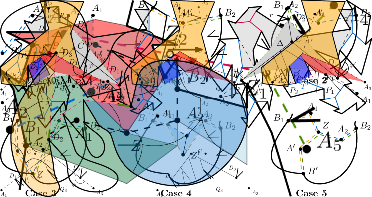
Figure 32: Modification as in Lemma 24. The pseudo-triangle $\Delta$ splits the polygon up into multiple sub-polygons, where we let $P_{1},P_{2},\ldots$ be those on the same “side” as the star-center $A_{1}$. Any partitions of $P_{1},P_{2},P_{3},\ldots$ can be extended to the polyline $D_{3}$-$C$-$D_{1}$ in such a way that $A$ sees the tripod point $C$.

Proof.

See Figure 32. We simply extend the boundaries of the pieces in $P_{i}$ touching the pseudo-triangle $\Delta$ until they meet the separator $D_{3}$-$C$-$D_{1}$. If two such boundaries meet during this process, we continue extending one of the boundaries while we let the other one end (the one to extend can be chosen arbitrarily).

We will handle the piece $Q_{1}$ with star center $A_{1}$ in a special manner, since we want it to see the tripod point $C$. So let $Z$ be the point on $\partial\Delta$ so that $Q_{1}$ contains the segment $D_{1}Z$ on this boundary. Then we extend the line $A_{1}Z$ until it meets the line $D_{3}C$ first, and assign this region to $Q_{1}$ (here we must use the fact that $C$ is a convex corner of $P^{\prime}$, by definition, so that $A_{1}$ indeed can see this region).

What remains is to argue that everything inside $\Delta$ is covered by our extended partition. This is true as long as the pseudo-diagonal between $D_{1}$ and $D_{3}$ contains no edge of $P$ (i.e. $\partial\Delta\cap\partial P$ just contains a finite amount of points, and no line segments). To argue this we use that $T$ was a tripod of some constructable solution. In particular this means that there exists some partition where $T$ is a tripod and no star center lies within the pseudo-triangle $\Delta$. Hence, if there was some edge $e$ of $P$ contained in $\partial\Delta$, then the interior of this edge could not be seen by any star center in such a constructable partition, which is our desired contradiction. ∎

5.2.1 Greedy Choice

Figure 33: Left: Two child star-centers $A_{1}$ and $A_{2}$ define a (fake) tripod with tripod point $C$, splitting the polygon into three subpolygons: “childs” $P_{1},P_{2}$, and “parent” $P_{3}$. The angle $\varphi=\angle CD_{3}D^{\prime}$ of this tripod is a measure on how “restricted” a potential star-center $A_{3}$ defined by this tripod is. Middle: Two other star centers $A^{\prime}_{1}$ and $A^{\prime}_{2}$ define another fake tripod on the same support, which is less restrictive (i.e., with an angle $\varphi^{\prime}<\varphi$). Inside $P_{3}$ (the parent-side of the tripod), the same partition is shown (in red and blue) as on the left. Right: The star partition of subpolygon $P_{3}$ can be adjusted (without moving any star centers) to also work with the less restrictive tripod.

Consider three concave corners $(D_{1},D_{2},D_{3})$ of $P$, that might support a tripod in some constructable partition. We now argue that if there are many possibilities for how the legs of a tripod supported by $(D_{1},D_{2},D_{3})$ look like, then it suffices to consider a single one of these possibilities! We will call this arrangement the greedy choice of this tripod. Recall that the tripod point is constructed by two of the sub-polygons $P_{1},P_{2}$, and used to define the third sub-polygon $P_{3}$ (see Figures 6 and 33). In particular, $P_{1}$ and $P_{2}$ are the children in the tripod tree (see Figure 19), and $P_{3}$ the parent. We argue that the greedy choice will be the combination of optimal solutions in the two subpolygons $P_{1}$ and $P_{2}$ that give rise to the least restrictive tripod-center when constructing the optimal solution for $P_{3}$. With least restrictive we mean the one that minimizes the angle $\varphi=\angle CD_{3}D^{\prime}$ as in Figure 33, as such a tripod will only impose the mildest restrictions on where the star center $A_{3}\in P_{3}$ participating in the tripod lies.

We begin by proving that it never hurts replacing a tripod with a less restrictive one, see also Figure 33.

Lemma 25.

Suppose that there is a tripod $\mathcal{T}$ with tripod point $C$ supported by three corners $(D_{1},D_{2},D_{3})$, part of a constructable partition $\mathcal{Q}$. Let $\Delta$ be the pseudo-triangle of the tripod, and consider the three sub-polygons $P_{1},P_{2},P_{3}$ in $P\setminus\Delta$ participating in the tripod, such that the parent star center of $\mathcal{T}$ is contained in $P_{3}$, as in Figures 33 and 6.

Suppose now that there is some other constructable sub-partitions of $P_{1}$ and $P_{2}$ (using the same number of star pieces as in the original one) giving rise to another fake tripod $\mathcal{T}^{\prime}$ (supported on the same three concave corners $D_{1},D_{2},D_{3}$) with tripod point $C^{\prime}$, that is less restrictive (the angle $\varphi$ in Figure 33 is smaller) for $P_{3}$. Then there also exists a constructable optimal star partition of $P$ that contains these new sub-partitions of $P_{1}$ and $P_{2}$, and the fake tripod $\mathcal{T}^{\prime}$.

Proof.

By Lemma 24, there exists an optimal partition $\mathcal{Q}^{\prime}$ containing the same sub-partition in $P_{1}$ and $P_{2}$ that gives $\mathcal{T}^{\prime}$. Since no star center is in the pseudo-triangle $\Delta$ of $\mathcal{T}$, the pseudo-triangle $\mathcal{T}^{\prime}$ is also constructable with respect to $\mathcal{Q}^{\prime}$. Our lemma then follows directly from Lemma 12. ∎

Greedy-constructable partitions.

By Lemma 25, it never hurts to replace a tripod with a less restrictive one. The next step is to argue that we can assume that all tripods in our constructable partition can follow such a greedy choice—which is a very useful property when designing an algorithm. This is a bit subtle, since such an algorithm might not actually find the least restrictive version of a tripod $\mathcal{T}$, but only the least restrictive version given that all children tripods also follow the greedy choice. We formalize this by the notion of greedy-constructable partitions. A greedy-constructable partition is constructable and also satisfies the following extra property, adding to properties (i)–(iv) of a constructable partition.

• Any tripod $\mathcal{T}$ in the partition is greedy (see Definition 26 below).

Definition 26 (Greedy Choice & Less Restrictive Tripods).

First, we define the angle of a fake tripod $\mathcal{T}$ as in Figure 33, i.e., the angle $\varphi=\angle CD_{3}D^{\prime}$, where $D^{\prime}$ is the next corner of $P$ after $D_{3}$, in the parent-subpolygon $P_{3}$. We say that a fake tripod $\mathcal{T}$ is less restrictive than another fake tripod $\mathcal{T}^{\prime}$ (supported by the same three corners) if the angle is smaller for $\mathcal{T}$ than for $\mathcal{T}^{\prime}$, i.e. if $\mathcal{T}$ imposes a weaker restriction on the potential star center in the parent subpolygon. We break ties in an arbitrary but consistent manner.

Consider a tripod $\mathcal{T}$ supported by corners $(D_{1},D_{2},D_{3})$ in some constructable partition. Suppose this tripod splits the polygon into the three sub-polygons $P_{1},P_{2},P_{3}$ and is oriented towards $P_{3}$. Consider all the pairs of greedy-constructable sub-partitions of $P_{1}$ and $P_{2}$, giving rise to some (fake) tripods $\mathcal{T}^{\prime}$ supported by the same corners $(D_{1},D_{2},D_{3})$. Then the tripod $T$ is the greedy choice for $(D_{1},D_{2},D_{3})$, or we simply say that $\mathcal{T}$ is greedy, if it is the least restrictive for $P_{3}$ among all such (fake) tripods $\mathcal{T}^{\prime}$.

Lemma 27.

There exists a greedy-constructable partition.

Proof.

The general idea is to start with a constructable partition (which exists by Theorem 10), and replace tripods that are not greedy by their greedy version instead, using Lemma 25. At first it might not be apparent that this will work, since Lemma 25 might introduce new tripods that are not greedy. We overcome this by carefully eliminating bad tripods in a bottom-up fashion, and continuing in a recursive manner, similar to our proof that there exists constructable partitions (proof of Theorem 10).

Formally, let us consider some polygon $P$ together with a constructablediscussion in partition $\mathcal{Q}$ of $P$. Throughout this proof, whenever we say tripod, we also consider fake tripods (see discussion in Sections 3.1 and 9)—i.e. those that can be constructed by two children star centers but might not be used to construct a parent star center. Consider the rooted tripod tree (see 8, 5 and 19) of this partition. In this tree we mark all tripods that are not greedy as bad, along with all ancestor tripods. Call this set of bad tripods $\mathcal{T}_{bad}(\mathcal{Q})$, and let $\mathcal{T}_{good}(\mathcal{Q})$ be all other tripods. That is $\mathcal{T}_{good}(\mathcal{Q})$ is the set of tripods $T$ in $\mathcal{Q}$ for which all tripods in the subtree rooted at $T$ (including $T$ itself) are greedy. If $\mathcal{T}_{bad}(\mathcal{Q})$ is empty, $\mathcal{Q}$ is greedy-constructable, so we are done; so suppose that this is not the case. Let $R(\mathcal{Q})$ be the region in $P$ reachable from the root edge $r$ without passing through any tripod from $\mathcal{T}_{good}(\mathcal{Q})$ (see also Figure 34). Note that all tripods in $\mathcal{T}_{bad}(\mathcal{Q})$ must by definition be in $R(\mathcal{Q})$. We will argue that we can find some other (constructable) partition $\mathcal{Q}^{\prime}$ such that $R(\mathcal{Q}^{\prime})$ is smaller. This is enough, since there are only finitely many possible positions for tripods in constructable solutions, so $R(\cdot)$ can only decrease a finite number of times.

Figure 34: The process of replacing a tripod $T$ with the greedy one $T^{\prime}$, as described in the proof of Lemma 27. Bad tripods $\mathcal{T}_{bad}$ are marked in red, good $\mathcal{T}_{good}$ in blue. The dashed lines indicates “fences” where star centers are not allowed to pass through. The gray area $R(\cdot)$ goes down, since the bad tripod $T$ was replaced with a good one $T^{\prime}$. The partitions (and tripods) inside $P_{1},P_{2}$ and $P^{\prime}_{3}=R(\mathcal{Q})\cap P_{3}$ can change: for example note that the tripods inside $P_{1}$ changed, and that a new bad tripod inside $R(\mathcal{Q}^{\prime})$ appeared.

Consider Figure 34. Let $T\in\mathcal{T}_{bad}(\mathcal{Q})$ be some non-greedy tripod. Say it is supported by corners $(D_{1},D_{2},D_{3})$ and splits the polygon into sub-polygons $P_{1},P_{2},P_{3}$ where it is oriented towards $P_{3}$. Without loss of generality, we may assume that, in our partition, the sub-partitions of $P_{1}$ and $P_{2}$ are greedy-constructable: that is all tripods in $P_{1}$ and $P_{2}$ abide the greedy choice (else we can instead choose $T$ to be one of these non-greedy tripods deeper down in the tripod tree). Since $T$ is not greedy, there must exist other sub-partitions of $P_{1}$ and $P_{2}$ that are also greedy-constructable and give rise to a better (less restrictive) greedy tripod $T^{\prime}$. First note that these new sub-partitions of $P_{1}$ and $P_{2}$ must use the same number of pieces as the original partition used for these sub-polygons (otherwise it was not optimal; note that it never makes sense to use an extra piece in a sub-partition to get a less restrictive tripod as we might as well place this extra piece at the tripod point which would make the whole tripod redundant).

Now we want to use Lemma 25 to replace the tripod $T$ with $T^{\prime}$. However, we cannot directly apply this lemma as it might destroy some greedy tripods and introduce new non-greedy tripods inside the region $P_{3}$ in an unpredictable manner. Let us define $P^{\prime}_{3}=P_{3}\cap R(\mathcal{Q})$ and $P^{\prime}=P_{1}\cup P_{2}\cup P^{\prime}_{3}$. We use Lemma 25 on the polygon $P^{\prime}$ instead of $P$, which makes sure that we do not destroy any greedy tripods inside the region $P_{3}$. We must be slightly careful also to not move any star centers into the pseudo-triangles of tripods in $P$, whose tripod points might now be corners of $P^{\prime}$. For this, we note that it is easy to extend Lemma 25 to take into account these pseudo-triangles:

In the first part of the proof of Lemma 25 we argued that there is an optimal (not necessarily constructable) solution without moving any star centers in $P^{\prime}_{3}$, and in the second part we used Theorem 10 (or rather Lemma 12) to argue that then there must also exist a constructable one. When we invoke Lemma 12 we can do so on the full polygon $P$, but on our partitions where everything outside $P_{3}^{\prime}$ is already constructable (so these star pieces and tripods will not change, and no star center will be moved into the pseudo-triangles of the boundary tripods of $P^{\prime}_{3}$). Then Lemma 12 would give us an optimal partition where tripods and star centers inside $P^{\prime}_{3}$ are also constructable.

To recap, we now have a constructable partition of $P^{\prime}$ where the greedy tripod $T^{\prime}$ is used instead of $T$. We extend this to a partition $\mathcal{Q}^{\prime}$ of $P$ by using all pieces from the original partition $\mathcal{Q}$ which where in $P\setminus P^{\prime}=P_{3}\setminus R(\mathcal{Q})$. By design we see that $\mathcal{Q}^{\prime}$ is constructable. Moreover, $R(\mathcal{Q^{\prime}})=P^{\prime}_{3}=R(\mathcal{Q})\cap P_{3}$, since now $T^{\prime}$ is a greedy tripod (and still all tripods in the subregions $P_{1}$ and $P_{2}$ are greedy, although the new partition of these parts can be quite different from the original one). To conclude, $R(\cdot)$ must have gone down, as it is now also restricted by the tripod $T^{\prime}$ (and the original tripod $T$ was completely contained in $R(\mathcal{Q})$). Hence, by induction, there must exist some greedy-constructable partition. ∎

5.2.2 Minimum Star Partition Algorithm

We are now ready to present the full algorithm, and thus proving Section 1. To optimally partition a polygon $P$ into a minimum number of star pieces we employ the following strategy. We begin by enumerating all possible positions for tripods (that is triples of concave corners $D_{1},D_{2},D_{3}$ of $P$ that might support a tripod). Now, for each of these, we can employ the greedy choice (see Definition 26) to only have a single tripod-center we need to consider. By Lemma 27, there must exist some optimal solution in which all tripods follow this greedy choice. For now, assume we can actually compute these greedy tripod points (we will get back to this later). That is we have $O(n^{3})$ potential tripod-centers in total. By Theorem 10 we can now construct a set of potential star centers $S^{\textsc{(centers)}}$ by considering all intersections of pairs of lines, where each line is either (i) an extension of a diagonal of $P$, or (ii) a line from a (greedy) tripod-center through the corresponding concave corner in this tripod. Note that there are only $O(n^{2}+n^{3})$ such lines, so we can bound $|S^{\textsc{(centers)}}|$ by $O(n^{6})$. Additionally, we note that in (greedy-)constructable partitions, each piece touches the boundary at some corner. Given $S^{\textsc{(centers)}}$, we can hence employ the dynamic programming algorithm (Algorithm 1, Theorem 19) to find a minumum star partition of the polygon $P$.

Resolving the greedy choice.

Now, let us return to the issue of actually determining the position of the greedy choice tripod point, of some tripod supported on concave corners $D_{1},D_{2},D_{3}$ of $P$. Let $P_{1},P_{2},P_{3}$ be the sub-regions (like in Figure 6), such that the tripod is oriented towards $P_{3}$. Note that $P_{1}$ and $P_{2}$ are defined by a diagonal of $P$ and not by the (so far unknown) tripod. Now, we can find greedy-constructable optimal solutions for $P_{1}$ and $P_{2}$ separately, by invoking our algorithm recursively (see also Figure 35): in the subpolygons we again enumerate all potential tripods, solve using the greedy choice, and invoke the dynamic program to obtain an optimal solution. Note that there are only $O(n^{2})$ subproblems, since each subproblem is defined by some diagonal between two concave corners of $P$ (here we use the fact that the tripods in a greed-constructable partition form a rooted tree). Moreover, our dynamic program allows us to find all possible positions of the star center $A_{1}$ in $P_{1}$ used to define the tripod. Indeed $A_{1}$ is the star center that sees a prefix of the pseudo-diagonal from $D_{1}$ to $D_{2}$, so we can find all possible positions of it by 22. Similarly for the star center $A_{2}$ in $P_{2}$. Therefore we may simply enumerate over all pairs of possibilities of $A_{1}$ and $A_{2}$ and choose the best valid one according to the greedy choice (Definition 26, see also Figures 6, 33 and 35). By Lemma 24, any partition we get here can be extended to a partition meeting the tripod legs. Conversely, any constructable partition with a tripod supported by $D_{1},D_{2}$ and $D_{3}$, is also a partition of $P\setminus\Delta$ (as no star center would be inside the pseudo-triangle $\Delta$; so we can apply Lemma 1 to carve out this part). Hence we do not loose or gain anything by restricting ourselves to finding optimal partitions restricted by the pseudo-diagonal, instead of restricted by the (so far unknown) tripod.

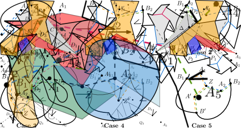
Figure 35: An illustration of how TripodGreedyChoice($D_{1},D_{2},D_{3}$) works. First the pseudo-triangle $\Delta$ (dashed in red) is computed. Then it calls SolveSubregion() on the yellow and blue subpolygons of $P\setminus\Delta$, to recursively partition these optimally. Moreover, using 22, we find all potential positions (in greedy-constructable optimal solutions) for star centers $A_{1}$ and $A_{2}$, whose piece contains a prefix (marked green in the figure) of the pseudo-diagonals adjacent to $D_{1}$ and $D_{2}$ (respectively). The pair which makes for the least restrictive (Definition 26) tripod point is chosen, and this point $C$ is returned. Curved parts indicated that details have been omitted.

Full algorithm.

The pseudo-code can be found in Algorithm 2, consisting of two mutually recursive functions TripodGreedyChoice() and SolveSubregion(). The function TripodGreedyChoice() will find the tripod point of the greedy tripod, and SolveSubregion($D_{1},D_{2}$) will optimally solve the sub-polygon enclosed by the diagonal $D_{1}$-$D_{2}$. To obtain the optimal partition for the full polygon, we can just call SolveSubregion() on some edge of $P$. The correctness follows from the above discussion.

1 function TripodGreedyChoice($D_{1},D_{2},D_{3}$):

       // Returns the greedy choice tripod point of the tripod supported by corners $D_{1},D_{2},D_{3}$ of $P$. See Figure 35.

       // Suppose, w.l.o.g. (other cases are similar), that we are like in Figure 6: that is the tripod should be oriented towards $D_{3}$ and the root is in the face fenced of by the $D_{2}$-$D_{3}$ pseudo-diagonal.

2       Construct the pseudo-diagonal $D_{1}$-$D_{2}$, say it goes through points $D_{1}=X_{1},X_{2},...,X_{k}=D_{2}$

3       Calculate the optimal number of star pieces to cover the sub-polygon defined by separator $X_{1}$-$X_{2}$, by calling SolveSubregion ($X_{1},X_{2}$)

4       Additionally, this finds all possible positions, in greedy constructable optimal solutions, of star centers that see a small part of the segment $X_{1}$-$X_{2}$ next to $D_{1}$

5       Do the same for diagonal $D_{2}$-$D_{3}$

6       Look at all combinations of star centers and return only the single tripod-center that makes for the greedy choice (if any).

7      

8

9

10function SolveSubregion($D_{1}$, $D_{2}$):

       // Requires that $D_{1},D_{2}$ is a diagonal of $P$. Call the sub-polygon on the right side (when looking from $D_{1}$ to $D_{2}$) of the diagonal $P^{\prime}$.

       // SolveSubregion ($D_{1},D_{2}$) will optimally partition $P^{\prime}$ into a minimum number of star-shaped pieces. Moreover, it will consider all possible positions, in greedy constructable solutions, for the star center that sees a small part of the $D_{1}D_{2}$ segment next to $D_{1}$.

11       Enumerate all valid positions of tripods (i.e. 3-tuples of concave corners) inside $P^{\prime}$, and call TripodGreedyChoice() on these.

12       Let $L$ be the set of lines that are either (i) the line through two corners of $P$, or (ii) the line through some tripod-center and the corresponding concave corner of $P$.

13       Let $S^{\textsc{(centers)}}$ be the set of intersection points of pairs of lines from $L$.

14       Call the dynamic programming algorithm on $P^{\prime}$ and $S^{\textsc{(centers)}}$ to find an optimal solution.

15       By 22 we can additionally find all possible positions of the star center seeing a prefix of the $D_{1}$-$D_{2}$ pseudo-diagonal from $D_{1}$ to $D_{2}$.

16      

17

Algorithm 2 Minimum Star Partition Algorithm.

Running time.

We now analyze the running time of Algorithm 2, and again we apply memoization to not recompute the same subpolygons multiple times. We will see that the total running time is $O(\mathrm{poly}(n))$—or, in fact $O(n^{107})$.

• TripodGreedyChoice() will be called at most $O(n^{3})$ times, since there are only $O(n^{3})$ choices for 3-tuples of corners $D_{1},D_{2},D_{3}$ of $P$. Constructing the pseudo-diagonals can be done in $O(n)$ time. There are at most $O(n^{6})$ possible positions for star centers, so only $O(n^{12})$ possible combinations for the greedy choice. For each of these combinations, we might need to go through the full polygon to see that the legs of the tripod does not intersect the polygon. Hence the computation inside TripodGreedyChoice() need in total $O(n^{3}\cdot n^{12}\cdot n)=O(n^{16})$ time over the run of the full algorithm.

• SolveSubregion() will be called at most $O(n^{2})$ times, since there are only $O(n^{2})$ choices for pairs of corners $D_{1},D_{2}$ of $P$. Enumerating valid tripod-positions can be done in $O(n^{4})$ time ($O(n^{3})$ many possible 3-tuples of corners, and each can be checked in $O(n)$ time by going through the polygon and constructing the pseudo-triangle to see if a valid tripod can be formed there). We then construct the set $S^{\textsc{(centers)}}$ of size at most $O(n^{6})$. Calling the dynamic programming algorithm on this set takes $O(n^{105})$ time (see Theorems 19 and 20). Followed from 22, in the same time, we can find all possible positions of star centers covering the start of the $D_{1}$-$D_{2}$ segment: indeed, we call the dynamic programming algorithm $\textnormal{{SolveSeparator}}(D_{1},A,X)$ (where $X\neq D_{1}$ is the closest point to $D_{1}$ in $S^{\textsc{(border)}}$ on the $D_{1}$-$D_{2}$ segment) for all possible star centers $A\in S^{\textsc{(centers)}}$, to see which ones of these give a partition of minimum size. Note that between these calls to SolveSeparator, we do not need to reset the dp-cache, so in total this takes only $O(n^{105})$ time. Hence, in total, over the full run of the algorithm, we will spend $O(n^{2}\cdot n^{105})=O(n^{107})$ time in SolveSubregion.

The above discussion concludes the proof of Section 1.

Appendix A Existence of Coordinate and Area Maximum Partitions

Proof of Lemma 3.

Recall that the Hausdorff distance between two compact sets $A,B\subset\mathbb{R}^{2}$ is defined as $d_{H}(A,B)\coloneqq\inf\{r\geq 0\mid A\subset B\oplus D(r)\text{ and }B\subset A\oplus D(r)\}$, where $\oplus$ is the Minkowski sum and $D(r)$ is the disk of radius $r$ centered at the origin. We will use the fact that $(M(\mathbb{R}^{2}),d_{H})$ is a compact metric space, where $M(\mathbb{R}^{2})$ denotes the set of all non-empty closed subsets of $\mathbb{R}^{2}$; see for instance [Eva08, Theorem 4.5].

Let $c^{*}=\sup c(\mathcal{Q})$, where the supremum is taken over all optimal star partitions $\mathcal{Q}$ of $P$. We claim there exists a star partition which realizes the coordinate vector $c^{*}$. Consider a sequence of optimal star partitions $(\mathcal{Q}_{i})_{i\in\mathbb{N}}$ so that $c(\mathcal{Q}_{i})$ converges to $c^{*}$ as $i\longrightarrow\infty$. Let $c(\mathcal{Q}_{i})=\langle A_{1i},\ldots,A_{ki}\rangle$ and let the pieces of $\mathcal{Q}_{i}$ be $Q_{1i},\ldots,Q_{ki}$ so that the maximum star center of $Q_{ji}$ is $A_{ji}$. Be passing to a subsequence, we can assume that the sequence $(Q_{1i})_{i\in\mathbb{N}}$ converges to a compact set $Q_{1}^{*}$ with respect to Hausdorff distance. Similarly, we can assume that $(Q_{ji})_{i\in\mathbb{N}}$ converges to $Q_{j}^{*}$ for each $j\in\{1,\ldots,k\}$. Let $\mathcal{Q}^{*}=\{Q_{1}^{*},\ldots,Q_{k}^{*}\}$ and $c^{*}=\langle A_{1}^{*},\ldots,A_{k}^{*}\rangle$. We claim that $\mathcal{Q}^{*}$ is a star partition of $P$ where $A_{j}^{*}$ is the star center of $Q_{j}^{*}$.

To see that $Q_{j}^{*}$ is star-shaped with star center $A_{j}^{*}$, we first observe that $A_{j}^{*}\in Q_{j}^{*}$. Otherwise, the star center $A_{ji}$ would not be in $Q_{ji}$ for sufficiently large values of $i$. Suppose now that $A_{j}^{*}$ is not a star center of $Q_{j}^{*}$. This means that there is a point $B\in Q_{j}^{*}$ so that the line segment $A_{j}^{*}B$ is not in $Q_{j}^{*}$. For each $i\in\mathbb{N}$, we can choose $B_{i}\in Q_{ji}$ so that $B_{i}\longrightarrow B$ for $i\longrightarrow\infty$. Since $A_{ji}\longrightarrow A_{j}^{*}$, $B_{i}\longrightarrow B$ and $A_{j}^{*}B$ is not in $Q_{j}^{*}$, it follows that $A_{ji}B_{i}$ is not in $Q_{ji}$ for sufficiently high values of $i$, which contradicts that $A_{ji}$ is a star center of $Q_{ji}$. In a similar way, we can argue that the sets in $\mathcal{Q}^{*}$ are interior-disjoint; otherwise, the sets in $\mathcal{Q}_{i}$ could not be interior-disjoint for sufficiently high values of $i$. Likewise, we get that $\bigcup\mathcal{Q}^{*}=P$, and we conclude that $\mathcal{Q}^{*}$ is a coordinate maximum optimal star partition of $P$. ∎

Proof sketch of Lemma 4.

The proof is analogous to that of Lemma 3. Without loss of generality, we can assume that $d=(1,0)$, so that for any set of points $A^{\prime}_{i},\ldots,A^{\prime}_{k}$, we have

$$\langle A^{\prime}_{i}\cdot d,A^{\prime}_{i}\cdot d^{\perp},A^{\prime}_{i+1}\cdot d,A^{\prime}_{i+1}\cdot d^{\perp},\ldots,A^{\prime}_{k}\cdot d,A^{\prime}_{k}\cdot d^{\perp}\rangle=\langle A^{\prime}_{i},A^{\prime}_{i+1},\ldots,A^{\prime}_{k}\rangle.$$

Define the supremum $\langle A^{*}_{i},A^{*}_{i+1},\ldots,A^{*}_{k}\rangle=\sup\langle A^{\prime}_{i},A^{\prime}_{i+1},\ldots,A^{\prime}_{k}\rangle$ over all partitions with star centers $A^{\prime}_{i},A^{\prime}_{i+1},\ldots,A^{\prime}_{k}$ in the region $F$ and the rest fixed at the points $A_{1},\ldots,A_{i-1}$. We then consider a convergent sequence of star partitions with fixed star centers $A_{1},\ldots,A_{i-1}$ and the rest converging to $A^{*}_{i},\ldots,A^{*}_{k}$, and it follows that the limit of the pieces constitute a partition realizing the supremum. ∎

Proof of Lemma 5.

The proof is similar to that of Lemma 3. Namely, let $a^{*}=\sup a(\mathcal{Q})$, where the supremum is taken over all star partitions $\mathcal{Q}$ of $P$ with star centers $\mathcal{A}$. We then consider a sequence of partitions $(\mathcal{Q}_{i})_{i\in\mathbb{N}}$ with star centers $\mathcal{A}$ so that $a(\mathcal{Q}_{i})\longrightarrow a^{*}$ as $i\longrightarrow\infty$. Let the pieces of $\mathcal{Q}_{i}$ be $Q_{1i},\ldots,Q_{ki}$ so that $A_{j}$ is a star center of $Q_{ji}$. By passing to a subsequence, we can assume that $(Q_{ji})_{i\in\mathbb{N}}$ converges to a compact set $Q_{j}^{*}$ for each $j\in\{1,\ldots,k\}$.

As in the proof of Lemma 3, we can conclude that $\mathcal{Q}^{*}=\{Q_{1}^{*},\ldots,Q_{k}^{*}\}$ is a star partition of $P$ with star centers $\mathcal{A}$ and that $a(\mathcal{Q}^{*})=a^{*}$, so $\mathcal{Q}^{*}$ is area maximum. ∎

Appendix B Structural Theorem

In this section, we give an elementary and independent proof of a structural theorem about optimal star partitions, which is not used in the rest of the paper. A point on the boundary of the polygon $P$ is canonical if it is a corner of $P$ or the endpoint of an extension of an edge of $P$; see Figure 36 (left).

Theorem 28.

Let $k$ be minimum such that there exists a star partition of $P$ consisting of $k$ polygons and assume $k\geq 2$. There exists a star partition $Q_{1},\ldots,Q_{k}$ of $P$, where each piece $Q_{i}$ has the following properties:

1. $\partial Q_{i}$ contains a concave corner of $P$, and

2. for each connected component of the shared boundary $\partial P\cap\partial Q_{i}$, both endpoints are canonical.

Figure 36: Left: A polygon with the extensions of the edges and the canonical points shown. Right: Using only canonical points as corners of pieces on the boundary of $P$, one of the points $C$ and $D$ must be used.

Before going into the proof, let us first make a few remarks. Note that there are at most $3n$ canonical points, since each edge of $P$ creates at most $2$ canonical points that are not corners of $P$. The algorithm described in this paper considers $O(n^{13})$ Steiner points on the boundary of $P$, so it might be possible to use property 2 to obtain a faster algorithm. However, in the proof of the theorem, we change the partition in order to only use canonical Steiner points on the boundary. It does therefore not follow immediately that our algorithm can also be modified to find the resulting partition, but we are confident that the result can be used to create a faster algorithm.

We find it somewhat surprising that canonical Steiner points suffice on the boundary of $P$, since, as shown in Figure 1, it is sometimes necessary to use Steiner points in the interior of $P$ of degree $\Omega(n)$, whereas the canonical points have degree at most $1$ (as defined in Section 1). Figure 36 (right) proves that it is necessary to have least some Steiner points on the boundary of $P$: In any partition into two star-shaped pieces, we must have a Steiner point on the segment $CD$.

Proof.

Let $Q_{1},\ldots,Q_{k}$ be a minimum star partition of $P$. Let us fix a star center $A_{i}$ in each piece $Q_{i}$. If $\partial Q_{i}\cap\partial Q_{j}\neq\emptyset$ and $i\neq j$, we say that $Q_{i}$ and $Q_{j}$ are neighbours. The shared boundary $\partial Q_{i}\cap\partial Q_{j}$ of two neighbours $Q_{i}$ and $Q_{j}$ is a collection of open polygonal curves. An interior point of an open curve is a point on the curve which is not an endpoint.

Claim 29.

Let $\gamma$ be an open curve in the shared boundary $\partial Q_{i}\cap\partial Q_{j}$ of two neighbours $Q_{i}$ and $Q_{j}$. We can assume that $\gamma$ is either a line segment or two line segments that have one of the star centers $A_{i}$ and $A_{j}$ as a common endpoint. If a star center of one piece is a corner of $\gamma$, the corner is convex with respect to that piece and concave with respect to the other piece.

Proof.

Figure 37: The process simplifying the shared boundary between $Q_{i}$ and $Q_{j}$ in order to satisfy 29. The gray region is the quadrilateral $F$.

Let the endpoints of $\gamma$ be $C$ and $D$; see Figure 37. Since the segments $A_{i}C$ and $A_{i}D$ are in $Q_{i}$, and $A_{j}C$ and $A_{j}D$ are in $Q_{j}$, we have a well-defined quadrilateral $F=A_{i}CA_{j}D$. If $A_{i}$ and $A_{j}$ are both convex corners of $F$, we replace $\gamma$ by the segment $CD$, which must be a diagonal of $F$. Otherwise, consider without loss of generality the case that $A_{i}$ is a concave corner of $F$. We then replace $\gamma$ by $CA_{i}\cup A_{i}D$. In either case, the modification clearly leaves $Q_{i}$ and $Q_{j}$ star-shaped, and we are left with a shared boundary of the claimed type. ∎

Property 1. In order to prove that there is a partition satisfying Property 1, suppose that $\partial Q_{i}$ does not contain a concave corner of $P$. We show how to modify the partition so that the property is eventually satisfied. In essence, we expand the piece $Q_{i}$ until Property 1 is eventually satisfied.

Claim 30.

We can assume that each concave corner $D$ of $Q_{i}$ is a concave corner of $P$ or a star center $A_{j}$ of a neighbour $Q_{j}$ of $Q_{i}$.

Proof.

We describe a way to expand $Q_{i}$ so that we eliminate concave corners of $Q_{i}$ which are neither corners of $P$ nor star centers of neighbours (note that if a concave corner of $Q_{i}$ touches $P$, then it touches $P$ at a concave corner). Let $CD$ and $DE$ be maximal segments on the boundary of $Q_{i}$ such that $D$ is a concave corner of $Q_{i}$ and no corner of $P$ and no star center of a neighbour is an interior point of $CD\cup DE$. It follows by 29 that this point $D$ can be assumed to lie on the boundary of two polygons $Q_{j}$ and $Q_{l}$ whose boundaries share a line segment $DF$. Informally, we now move $D$ towards $F$. This will expand $Q_{i}$ and shrink $Q_{j}$ and $Q_{l}$ and possibly also other neighbours of $Q_{i}$ whose boundaries contain segments or points on $CD\cup DE$. To be precise, define $D^{\prime}$ to be the first point on $DF$ from $D$ such that one of the following cases holds: (i) one of the segments $CD^{\prime}$ or $D^{\prime}E$ contains a corner of $P$, (ii) $D^{\prime}$ is the intersection of $DF$ and $CE$ (if it exists), (iii) one of the segments $CD^{\prime}$ or $D^{\prime}E$ contains a star center $A_{m}$, $m\neq i$, (iv) $D^{\prime}=F$. The cases are shown in Figure 38. We then assign the quadrilateral $CD^{\prime}ED$ to $Q_{i}$, which will increase $Q_{i}$, decrease the pieces intersected by $CD^{\prime}\cup D^{\prime}E$ and, by Lemma 1, all the involved pieces remain star-shaped. We repeat this operation, and it remains to argue that the process eventually terminates.

Figure 38: The process of eliminating concave corners of $Q_{i}$ that are not star centers of neighbouring pieces.

In case (i), $Q_{i}$ now touches $P$ at a corner which clearly must be concave. In case (ii), we have eliminated a concave corner of $Q_{i}$. In case (iii), we have increased the number of star centers on the boundary of $Q_{i}$, which can happen at most $k-1$ times. In case (iv), we eliminated a segment $DF$ of $Q_{j}$ and $Q_{l}$, which decreases the total number of segments of the pieces. We conclude that the operation can be repeated at most a finite number of times and the process therefore eventually terminates. ∎

A star neighbour of $Q_{i}$ is a neighbour $Q_{j}$ whose star center $A_{j}$ is on $\partial Q_{i}$. Recall that we assume $\partial Q_{i}$ does not contain a concave corner of $P$. Now, additionally assume that $Q_{i}$ is non-convex, i.e., $Q_{i}$ has a concave corner. As $\partial Q_{i}$ does not contain a concave corner of $P$, we can assume that this concave corner is the star center of a star neighbour by 30. To obtain a contradiction with the minimality of the start partition, we show that $Q_{i}$ can be subsumed by the star neighbours. To this end, we consider a triangulation of $Q_{i}$. The diagonals of the triangulation that have an endpoint at a concave corner of $Q_{i}$ partition $Q_{i}$ into convex polygons $R_{1},\ldots,R_{m}$, as illustrated in Figure 39 (left), where solid diagonals have an endpoint at a concave corner.

Figure 39: Left: We reassign the piece $Q_{i}$ to the pieces of the concave star neighbours. Right: We expand the convex piece $Q_{i}$ by adding the triangle $A_{j}CD$.

We assign a polygon $R_{p}$ to $Q_{j}$ if $A_{j}$ is on the boundary of $R_{p}$ and $R_{p}$ has not already been assigned to another star neighbour, as shown by the arrows in the figure. Thus, the considered star partition did not consist of a minimum number of polygons, which is a contradiction. Consequently, $Q_{i}$ must be convex.

As we assume $k\geq 2$, there has to be a piece $Q_{j}$ that is a neighbour of $Q_{i}$ so that the common boundary $\partial Q_{i}\cap\partial Q_{j}$ contains a segment $CD$. We expand $Q_{i}$ and shrink $Q_{j}$ by adding the triangle $A_{j}CD$ to $Q_{i}$, as shown in Figure 39 (right), which keeps $Q_{i}$ as well as $Q_{j}$ star-shaped. This can introduce concave corners $C$ and $D$ on $Q_{i}$, but we can proceed as in the proof of 30 and expand $Q_{i}$ until we hit a concave corner of $P$ or obtain that all concave corners are star centers. If we do not hit a concave corner of $P$, we can again argue that $Q_{i}$ can be subsumed by $Q_{j}$ and potentially other star neighbours, contradicting the minimality of the star partition.

Note that if a concave corner of $P$ appears on the boundary of a piece before the changes described above (including in the proof of 30), then the corner also appears on the piece afterwards. We conclude that we can expand each polygon $Q_{i}$ that does not contain a concave corner of $P$ until it eventually does. In the end, we obtain a minimum star partition with Property 1.

Property 2. We now prove that we can obtain Property 2. Consider an edge $CD$ of $P$. For each piece $Q_{i}$, it holds by the optimality of the partition that the intersection $CD\cap\partial Q_{i}$ is either empty or a single segment $EF$ (which may be a single point); see Figure 40. We call such a segment $EF$ a shared segment, and we say that a shared segment is canonical if both endpoints are canonical. We define the canonical prefix of $CD$ to be all the shared segments from $C$ to (and excluding) the first non-canonical shared segment. We show that we can modify the partition such that the number of segments in the canonical prefix increases. It therefore holds that the process must stop, so that all shared segments on $CD$ have canonical endpoints in the end. The process does not change whether shared segments on other edges of $P$ are canonical, so repeating the process for all edges yields a star partition with Property 2.

Figure 40: The fat segments are edges of $P$ and the thin black segments indicate the boundaries of pieces in the interior of $P$. The corners $C$ and $D$ as well as the interior points $E$ and $F$ are canonical, but $G$ is not. There are three segments in the canonical prefix of $CD$, namely the intersections of $CD$ with each of $\partial Q_{1},\partial Q_{2},\partial Q_{3}$.

Consider the first non-canonical segment $EF$, where $E$ is canonical but $F$ is not. Let $F^{\prime}$ be the first point on $FD$ from $F$ such that either (i) $F^{\prime}$ is canonical, (ii) $A_{i}F^{\prime}$ contains another star center $A_{j}$, or (iii) $A_{i}F^{\prime}$ contains a corner $G$ of $P$. Since the endpoint $D$ is canonical, the point $F^{\prime}$ is well-defined. The cases are illustrated in Figures 41, 42 and 43.

In case (i), we assign the triangle $A_{i}FF^{\prime}$ to $Q_{i}$, which according to Lemma 1 keeps all pieces star-shaped as the triangle does not contain any star centers of other pieces than $Q_{i}$. We have then increased the number of segments in the canonical prefix.

In case (ii), we assign the triangle $A_{i}EF^{\prime}$ to the piece $Q_{j}$. The shared segment $s=CD\cap\partial Q_{j}$ of the piece $Q_{j}$ now starts at the point $E$. The other endpoint of $s$ is either $F^{\prime}$ (as in Figure 41) or a later point. In the latter case, it is possible that $s$ is canonical, and we have increased the number of segments in the canonical prefix. If $s$ is not canonical, we repeat the process of repairing the non-canonical endpoint of $s$. Since the star center $A_{j}$ must be closer to the edge $CD$ than $A_{i}$, we encounter case (ii) less than $k$ times before we end in case (i) or (iii).

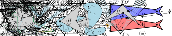
Figure 41: Case (i). We expand $Q_{i}$ with the triangle $A_{i}FF^{\prime}$.

Figure 42: Case (ii). We expand $Q_{j}$ with the triangle $A_{i}FF^{\prime}$.

It remains to consider case (iii), namely that $A_{i}F^{\prime}$ contains a corner $G$ of $P$. We know that $G\neq D$, since otherwise, we would have been in case (i). Let $F^{\prime\prime}$ be the first canonical point on the segment $F^{\prime}E$ from $F^{\prime}$, which is well-defined as $E$ is canonical. Furthermore, we know that $F^{\prime\prime}$ is on the segment $EF$, since otherwise, we should have been in case (i). Let $\mathcal{Q}^{\prime}=\{Q^{\prime}_{1},\ldots,Q^{\prime}_{f^{\prime}}\}\setminus\{Q_{i}\}$ be the set of pieces intersected by the interior of $GF^{\prime}$ in order from $G$ and excluding $Q_{i}$.

In a first step, we assign the triangle $A_{i}F^{\prime\prime}F^{\prime}$ to the piece $Q_{i}$. This can reduce pieces intersecting $A_{i}F^{\prime}$, but Lemma 1 ensures that they remain star-shaped. However, the point $F^{\prime}$ need not be canonical. In a second step, we therefore remove the triangle $\Delta=GF^{\prime\prime}F^{\prime}$ from $A_{i}$ and instead distribute $\Delta$ among the pieces $\mathcal{Q}^{\prime}$, as follows. For each $j=1,\ldots,f^{\prime}-1$, we consider the segment $s$ on the shared boundary of $Q^{\prime}_{j}$ and $Q^{\prime}_{j+1}$ with an endpoint on $GF^{\prime}$. We then extend $s$ into $\Delta$ until we reach one of the other segments $GF^{\prime\prime}$ or $F^{\prime\prime}F^{\prime}$ bounding $\Delta$, or we meet an extension that was already added for a smaller value of $j$. Since $F^{\prime\prime}$ was chosen as the first canonical point on $F^{\prime}E$, this results in a star partition of $P$. Furthermore, the shared segment of $Q_{i}$ on $CD$ has now become the segment $EF^{\prime\prime}$ (which might just be a single point), which is canonical, so we have increased the number of segments in the canonical prefix. Recall that we consider the number of segments in the prefix here and not the geometric length of the prefix; the geometric length of the prefix indeed can decrease.

Figure 43: Case (iii). In two steps, we distribute the triangle $A_{i}F^{\prime\prime}F^{\prime}$ among $Q_{i}$ and the pieces $Q^{\prime\prime}_{1},Q^{\prime\prime}_{2},Q^{\prime\prime}_{3}$ intersected by $GF^{\prime}$.

Finally, note that none of the above modifications of the star partition cause a piece $Q$ to become non-adjacent to a concave corner $H$ of $P$ if $Q$ was adjacent to $H$ before. More precisely, only the modifications in case (iii) changes the neighbourhood of a corner $G$ of $P$. However, as there are no star centers in the triangle $A_{i}EF^{\prime}$, the modifications will not remove $G$ from the boundary of any piece. ∎

References

- [AAE+17] Hugo A. Akitaya, Greg Aloupis, Jeff Erickson and Csaba D. Tóth “Recognizing Weakly Simple Polygons” In Discret. Comput. Geom. 58.4, 2017, pp. 785–821 DOI: 10.1007/s00454-017-9918-3
- [AAI86] Takao Asano, Tetsuo Asano and Hiroshi Imai “Partitioning a polygonal region into trapezoids” In J. ACM 33.2, 1986, pp. 290–312 DOI: 10.1145/5383.5387
- [AAM22] Mikkel Abrahamsen, Anna Adamaszek and Tillmann Miltzow “The Art Gallery Problem is -complete” In J. ACM 69.1, 2022, pp. 4:1–4:70 DOI: 10.1145/3486220
- [AAP86] Takao Asano, Tetsuo Asano and Ron Y. Pinter “Polygon Triangulation: Efficiency and Minimality” In J. Algorithms 7.2, 1986, pp. 221–231 DOI: 10.1016/0196-6774(86)90005-2
- [Abr21] Mikkel Abrahamsen “Covering Polygons is Even Harder” In 62nd IEEE Annual Symposium on Foundations of Computer Science (FOCS 2021), 2021, pp. 375–386 DOI: 10.1109/FOCS52979.2021.00045
- [ADG+20] Esther M. Arkin, Rathish Das, Jie Gao, Mayank Goswami, Joseph S.. Mitchell, Valentin Polishchuk and Csaba D. Tóth “Cutting Polygons into Small Pieces with Chords: Laser-Based Localization” In 28th Annual European Symposium on Algorithms (ESA 2020), 2020, pp. 7:1–7:23 DOI: 10.4230/LIPIcs.ESA.2020.7
- [AT81] David Avis and Godfried T. Toussaint “An efficient algorithm for decomposing a polygon into star-shaped polygons” In Pattern Recognit. 13.6, 1981, pp. 395–398 DOI: 10.1016/0031-3203(81)90002-9
- [BD92] Chandrajit L. Bajaj and Tamal K. Dey “Convex Decomposition of Polyhedra and Robustness” In SIAM J. Comput. 21.2, 1992, pp. 339–364 DOI: 10.1137/0221025
- [BFB12] Avisekh Banerjee, Hsi-Yung Feng and Evgueni V. Bordatchev “Process planning for Floor machining of 2D pockets based on a morphed spiral tool path pattern” In Computers & Industrial Engineering 63.4, 2012, pp. 971–979 DOI: 10.1016/j.cie.2012.06.008
- [BS03] Michael B. Bieterman and Donald R. Sandstrom “A curvilinear tool-path method for pocket machining” In J. Manuf. Sci. Eng. 125.4, 2003, pp. 709–715 DOI: 10.1115/1.1596579
- [BS21] Maike Buchin and Leonie Selbach “Decomposing Polygons into Fat Components” In 33rd Canadian Conference on Computational Geometry (CCCG 2021), 2021, pp. 175–184
- [CD85] Bernard Chazelle and David P. Dobkin “Optimal convex decompositions” In Computational Geometry 2, Machine Intelligence and Pattern Recognition, 1985, pp. 63–133 DOI: 10.1016/B978-0-444-87806-9.50009-8
- [CEX15] Hsien-Chih Chang, Jeff Erickson and Chao Xu “Detecting Weakly Simple Polygons” In Twenty-Sixth Annual ACM-SIAM Symposium on Discrete Algorithms (SODA 2015), 2015, pp. 1655–1670 DOI: 10.1137/1.9781611973730.110
- [Cha80] Bernard Chazelle “Computational geometry and convexity”, 1980
- [Cha82] Bernard Chazelle “A Theorem on Polygon Cutting with Applications” In 23rd Annual Symposium on Foundations of Computer Science (FOCS 1982), 1982, pp. 339–349 DOI: 10.1109/SFCS.1982.58
- [Cha84] Bernard Chazelle “Convex Partitions of Polyhedra: A Lower Bound and Worst-Case Optimal Algorithm” In SIAM J. Comput. 13.3, 1984, pp. 488–507 DOI: 10.1137/0213031
- [Cha87] Bernard Chazelle “Approximation and decomposition of shapes” In Algorithmic and Geometric Aspects of Robotics 1, Advances in Robotics, 1987, pp. 145–185
- [Cha91] Bernard Chazelle “Triangulating a Simple Polygon in Linear Time” In Discret. Comput. Geom. 6, 1991, pp. 485–524 DOI: 10.1007/BF02574703
- [Chv75] Vasek Chvátal “A combinatorial theorem in plane geometry” In J. Comb. Theory, Ser. B 18.1, 1975, pp. 39–41 DOI: 10.1016/0095-8956(75)90061-1
- [CP94] Bernard Chazelle and Leonidas Palios “Decomposition algorithms in geometry” In Algebraic Geometry and its applications, 1994, pp. 419–447 DOI: 10.1007/978-1-4612-2628-4˙27
- [CP97] Bernard Chazelle and Leonidas Palios “Decomposing the Boundary of a Nonconvex Polyhedron” In Algorithmica 17.3, 1997, pp. 245–265 DOI: 10.1007/BF02523191
- [Dam04] Mirela Damian “Exact and approximation algorithms for computing optimal fat decompositions” In Comput. Geom. 28.1, 2004, pp. 19–27 DOI: 10.1016/j.comgeo.2004.01.004
- [DKB13] Andrew Dobson, Athanasios Krontiris and Kostas E. Bekris “Sparse roadmap spanners” In Algorithmic Foundations of Robotics X (WAFR 2013), 2013, pp. 279–296 DOI: 10.1007/978-3-642-36279-8˙17
- [DO03] Mirela Damian-Iordache and Joseph O’Rourke “Partitioning Regular Polygons into Circular Pieces I: Convex Partitions” In Proceedings of the 15th Canadian Conference on Computational Geometry (CCCG 2003), 2003, pp. 43–46 URL: http://www.cccg.ca/proceedings/2003/27.pdf
- [DP04] Mirela Damian and Sriram V. Pemmaraju “Computing Optimal Diameter-Bounded Polygon Partitions” In Algorithmica 40.1, 2004, pp. 1–14 DOI: 10.1007/s00453-004-1092-3
- [ER97] Michal Etzion and Ari Rappoport “On compatible star decompositions of simple polygons” In IEEE Transactions on Visualization and Computer Graphics 3.1, 1997, pp. 87–95 DOI: 10.1109/2945.582388
- [Eva08] Steven N. Evans “Probability and real trees”, Lecture notes in mathematics 1920 Springer, 2008 DOI: 10.1007/978-3-540-74798-7
- [Fis78] Steve Fisk “A short proof of Chvátal’s Watchman Theorem” In J. Comb. Theory, Ser. B 24.3, 1978, pp. 374 DOI: 10.1016/0095-8956(78)90059-X
- [FP75] Hou-Yuan F. Feng and Theodosios Pavlidis “Decomposition of Polygons Into Simpler Components: Feature Generation for Syntactic Pattern Recognition” In IEEE Trans. Computers 24.6, 1975, pp. 636–650 DOI: 10.1109/T-C.1975.224276
- [GJP+78] M.. Garey, David S. Johnson, Franco P. Preparata and Robert Endre Tarjan “Triangulating a Simple Polygon” In Inf. Process. Lett. 7.4, 1978, pp. 175–179 DOI: 10.1016/0020-0190(78)90062-5
- [HM85] Stefan Hertel and Kurt Mehlhorn “Fast Triangulation of the Plane with Respect to Simple Polygons” In Inf. Control. 64.1-3, 1985, pp. 52–76 DOI: 10.1016/S0019-9958(85)80044-9
- [Kei85] J. Keil “Decomposing a Polygon into Simpler Components” In SIAM J. Comput. 14.4, 1985, pp. 799–817 DOI: 10.1137/0214056
- [Kei99] J. Keil “Polygon decomposition” In Handbook of computational geometry, 1999, pp. 491–518 DOI: 10.1016/B978-044482537-7/50012-7
- [Kre98] Marc J. Kreveld “On fat partitioning, fat covering and the union size of polygons” In Comput. Geom. 9.4, 1998, pp. 197–210 DOI: 10.1016/S0925-7721(96)00016-8
- [KS02] J. Keil and Jack Snoeyink “On the Time Bound for Convex Decomposition of Simple Polygons” In Int. J. Comput. Geom. Appl. 12.3, 2002, pp. 181–192 DOI: 10.1142/S0218195902000803
- [KS85] J. Keil and Jörg-R. Sack “Minimum Decompositions of Polygonal Objects” In Computational Geometry 2, Machine Intelligence and Pattern Recognition, 1985, pp. 197–216 DOI: 10.1016/B978-0-444-87806-9.50012-8
- [Lie07] Jyh-Ming Lien “Approximate Star-Shaped Decomposition of Point Set Data” In Eurographics Symposium on Point-Based Graphics (PBG 2007), 2007 DOI: 10.2312/SPBG/SPBG07/073-080
- [LL09] Jyh-Ming Lien and Yanyan Lu “Planning motion in point-represented contact spaces using approximate star-shaped decomposition” In IEEE/RSJ International Conference on Intelligent Robots and Systems (IROS 2009), 2009, pp. 5420–5425 DOI: 10.1109/IROS.2009.5354685
- [LN88] Robin Liu and Simeon C. Ntafos “On Decomposing Polygons into Uniformly Monotone Parts” In Inf. Process. Lett. 27.2, 1988, pp. 85–89 DOI: 10.1016/0020-0190(88)90097-X
- [LN91] Robon Liu and Simeon C. Ntafos “On Partitioning Rectilinear Polygons into Star-Shaped Polygons” In Algorithmica 6.6, 1991, pp. 771–800 DOI: 10.1007/BF01759071
- [Lub85] Anna Lubiw “Decomposing polygonal regions into convex quadrilaterals” In First Annual Symposium on Computational Geometry (SoCG 1985), 1985, pp. 97–106 DOI: 10.1145/323233.323247
- [MW97] Matthias Müller-Hannemann and Karsten Weihe “Minimum Strictly Convex Quadrangulations of Convex Polygons” In Thirteenth Annual Symposium on Computational Geometry (SoCG 1997), 1997, pp. 193–202 DOI: 10.1145/262839.262960
- [ORo87] Joseph O’Rourke “Art Gallery Theorems and Algorithms” Oxford University Press, 1987
- [OS83] Joseph O’Rourke and Kenneth J. Supowit “Some NP-hard polygon decomposition problems” In IEEE Trans. Inf. Theory 29.2, 1983, pp. 181–189 DOI: 10.1109/TIT.1983.1056648
- [OST18] Joseph O’Rourke, Subash Suri and Csaba D. Tóth “Polygons” In Handbook of discrete and computational geometry, 2018, pp. 787–810 DOI: 10.1201/9781315119601
- [PL19] Divyangkumar D. Patel and Devdas I. Lalwani “Effect of algorithm parameters in development of spiral tool path for machining of 2.5D star-shaped pockets” In International Journal of Computer Aided Engineering and Technology 11.6, 2019, pp. 727–746 DOI: 10.1504/IJCAET.2019.102501
- [Sch78] Bruce J. Schachter “Decomposition of Polygons into Convex Sets” In IEEE Trans. Computers 27.11, 1978, pp. 1078–1082 DOI: 10.1109/TC.1978.1675001
- [She92] Thomas C. Shermer “Recent results in art galleries” In Proc. IEEE 80.9, 1992, pp. 1384–1399 DOI: 10.1109/5.163407
- [SR95] Michal Shapira and Ari Rappoport “Shape blending using the star-skeleton representation” In IEEE Computer Graphics and Applications 15.2, 1995, pp. 44–50 DOI: 10.1109/38.365005
- [Tou82] Godfried T. Toussaint “Computational geometric problems in pattern recognition” In Pattern Recognition Theory and Applications: Proceedings of the NATO Advanced Study Institute, 1982, pp. 73–91 DOI: 10.1007/978-94-009-7772-3˙7
- [VM05] Gokul Varadhan and Dinesh Manocha “Star-shaped Roadmaps – A Deterministic Sampling Approach for Complete Motion Planning” In Robotics: Science and Systems (RSS 2005), 2005 DOI: 10.15607/RSS.2005.I.004
- [XHH+10] Jiazhi Xia, Ying He, Shuchu Han, Chi-Wing Fu, Feng Luo and Xianfeng Gu “Parameterization of star-shaped volumes using Green’s functions” In Advances in Geometric Modeling and Processing (GMP 2010), 2010, pp. 219–235 DOI: 10.1007/978-3-642-13411-1˙15
- [YL11] Wuyi Yu and Xin Li “Computing 3D shape guarding and star decomposition” In Computer Graphics Forum 30.7, 2011, pp. 2087–2096 DOI: 10.1111/j.1467-8659.2011.02056.x
- [ZKV+06] Liangjun Zhang, Young J. Kim, Gokul Varadhan and Dinesh Manocha “Fast C-obstacle query computation for motion planning” In IEEE International Conference on Robotics and Automation (ICRA 2006), 2006, pp. 3035–3040 DOI: 10.1109/ROBOT.2006.1642163