Growth-rate distributions of gut microbiota time series: neutral models and temporal dependence

Abstract

Logarithmic growth-rates are fundamental observables for describing ecological systems and the characterization of their distributions with analytical techniques can greatly improve their comprehension. Here a neutral model based on a stochastic differential equation with demographic noise, which presents a closed form for these distributions, is used to describe the population dynamics of microbiota. Results show that this model can successfully reproduce the log-growth rate distribution of the considered abundance time-series. More significantly, it predicts its temporal dependence, by reproducing its kurtosis evolution when the time lag $\tau$ is increased. Furthermore, its typical shape for large $\tau$ is assessed, verifying that the distribution variance does not diverge with $\tau$. The simulated processes generated by the calibrated stochastic equation and the analysis of each time-series, taken one by one, provided additional support for our approach.

Alternatively, we tried to describe our dataset by using a logistic model with an environmental stochastic term. Analytical and numerical results show that this model is not suited for describing the leptokurtic log-growth rates distribution found in our data. These results effectively support a neutral model with demographic stochasticity for describing the growth-rate dynamics and the stationary abundance distribution of the considered microbiota. This suggests that there are no significant parametric demographic differences among the species, which can be statistically characterized by the same vital rates.

1 Introduction

Quantitative studies of gut microbiota have generated an increasing and rich body of information about different features of these ecosystems. This has been made possible by the fact that nowadays these microbial communities present a more experimental accessibility than other macroscopic ecological communities, as current sequencing technologies can monitor with high temporal resolution the dynamics of abundance of bacteria [1]. Numerous studies have described some aspects of the community ecology of these systems. They outlined macroecological patterns that characterize global statistical relationships of spatial and temporal variation and taxonomical diversity [2, 3, 4] and even their temporal changes associated with host health, diet and lifestyle [5]. However, a robust and general description of gut microbiota at the level of population dynamics is still missing. Therefore, it is interesting and important to identify quantitative statistical stylized facts which can characterize the population dynamics of gut bacteria, with the ultimate goal of pointing out the biological processes and factors governing these dynamics.

In this work we will focus on the population dynamics displayed by the different species of bacteria present in gut microbiota. A very important observable used in the description of population dynamics is the logarithmic growth rate. Given an abundance time series $x(t)$, the log-growth rate is defined as: $g(t,\tau)=\ln{x(t+\tau)}-\ln{x(t)}$. The time series of this quantity have been traditionally used in population dynamics for analyzing important features of the corresponding populations. Some analysis methods proposed by Royama [6] are capable of generating clear diagnoses of their ecological features, in particular density dependence. This phenomenological approach is based on the fit of the population growth rate and it is more efficient in testing and diagnosing, rather than in modeling [7, 8].

The idea behind the use of this quantity, instead of directly considering abundance time series, is linked to the construction of an observable close to stationarity. In fact, abundances are frequently non-stationary and subject to large variations and measurement errors. It follows that it is more robust to consider the fluctuations of the observable, measured as the difference between two consecutive logarithms of the abundance. Indeed, if the process has multiplicative dynamics, logarithms are a natural choice because they eliminate underlying exponential growth trends. Finally, it is interesting to note that this observable has been traditionally associated with a discrete approximation for the instantaneous population per capita growth rate, since $\ln(x(t+1))-\ln(x(t))\approx\frac{1}{x}\frac{dx}{dt}$ in a first, rough approximation.

In this study we will focus on the characterization of the $P(g,\tau)$, the distribution of the $g(t,\tau)$ when the process has reached stationarity. This distribution has been already studied for the microbiota by Ji et al. [9]. Moreover, it has been actively investigated not only in other ecological systems [10], but also in finance (the return distribution) [15], economics [11, 12, 13] and social science [14]. There, the considered underlying observables were not population abundances but, respectively, prices, firms and fund sizes, and crimes.

Early simple multiplicative models, discrete or continuous, hypothesized that the Gaussian distribution should emerge as a typical shape modeling this distribution. In contrast, empirical studies showed that, generally, $P(g,\tau)$ are not simply characterized by Gaussian distributions, but it is common to find shapes close to the Laplace distribution [10, 11, 14] or, in finance, distributions with power-law tails [15, 16]. There is a second, important, statistical feature characterizing the temporal dependence of the shape of $P(g,\tau)$. $P(g,\tau)$ is markedly dependent on $\tau$ and seems to be attracted towards a Gaussian shape for increasing values of this parameter. This last behavior is well known in finance [15, 13], where it is called aggregational gaussianity and it is justified on the basis of the central limit theorem. As $g(t,\tau)$ is time additive, for independent data points, the distribution is expected to converge to a Gaussian one for large $\tau$.

In this study we will characterize $P(g,\tau)$ and its temporal dependence by using a stochastic model which describes the underlying abundance time series [17]. This method allows to analytically obtain the $P(g,\tau)$ and its temporal dependence and to compare them with the empirical data. In addition to the description of the principal features of the log-growth rate distribution, this approach suggests a specific model of population dynamics for the species present in the considered microbiota. This model is part of a class of models which describe ecological systems within a neutral framework. Neutral theories [18, 19] posit that the dominant factors that determine the structures of an ecological community are driven by the demographic randomness present in the populations, which determine their random drift. By contrast, the selection produced by the interactions among the individuals, the species identity and the environment effects are considered far less relevant. In its more universal implementation, the neutral theory of biodiversity models the organisms of a community with identical per capita death, birth, immigration and speciation rates [18]. Species are considered demographically and ecologically equivalent and characterized by the same demographic rates. Among the different models generated by these ideas, we consider a very simple and general one, based on a stochastic differential equation (SDE) which describes the dynamics of the population density. It is driven by a linear drift and the noise term includes the square root of the population density, which describes demographic noise [17]. This approach generates predictions at stationarity, which have been successfully applied in a variety of different systems, such as [20] .

With the aim of introducing some comparisons between the statistical patterns generated by different approaches, we consider a second model recently used for describing population dynamics in microbiota [21, 22]. In this approach, populations are modeled by a traditional logistic growth term, coupled with a source of environmental stochasticity implemented by a simple multiplicative term. In the next section these two models will be described in detail.

2 Data

In recent times microbiome data have become increasingly accessible and a variety of different datasets have been analyzed in several studies. Here we focus on the dataset previously considered by Zaoli et al. [22]. As we are interested in the population dynamics of the bacterial abundance, and not in the characterization of the community ecology, we look for data focusing on their statistical robustness rather than worrying about their generality. For this reason, we select time-series presenting daily sampling frequency, and a density of data points different from 0 of at least 75%. We end up with data from four healthy human individuals: 2 individuals (M3 and F4) from the Moving Pictures MP dataset [23], and the time-series of the post-travel period of individual A and the pre-Salmonella interval of individual B of the study of David et al. [5]. This dataset corresponds to a total of 1305 abundance time-series of bacterial operational taxonomical unit (OTU). In this time-series non-stationarity is a relative common issue. For reasons of statistical analysis and taking into account our modeling approach, only stationary series are taken into account. These series are selected by using the Dickey-Fuller test and correspond to 75% of the original dataset.

3 Methods

The neutral framework can be implemented by describing the abundance dynamics $x(t)$ with the following SDE:

$$dx_{t}=(b-x_{t}/a)dt+\sqrt{2Dx_{t}}dW_{t},$$ (1)

where $a,b,D>0$ and $W_{t}$ is a standard Wiener process. The solution of this equation is a randomly fluctuating population which is drawn back to a long-term deterministic value equal to $ab$, with a correlation time determined by $a$ and fluctuations controlled by the parameter $D$. This SDE is known in the literature as the Cox-Ingersoll-Ross (CIR) equation. It was first introduced by Feller for modeling population growth [24] and, following its use to model interest rates [25], it became very popular in the finance literature. More recently, it has been adopted for describing Neutral dynamics in ecological systems [17] and we consider this interpretation as the theoretical underpinning of its use in this work. This equation has an explicit solution. The propagator can be also analytically obtained and the stationary distribution is given by the Gamma distribution:

$$P(x)=\frac{x^{\alpha-1}e^{-x/Da}}{\Gamma(\alpha)(Da)^{\alpha}},$$ (2)

where we introduce the notation $\alpha=b/D$. Despite this process has been frequently used in finance, where returns are a fundamental measure, only recently an analytical result have been obtained for describing the log-growth rate distributions $P(g,\tau)$ [17]. Following Azaele et al. [17], this distribution can be obtained starting from the conditional transition density and the stationary probability distribution, which allows to calculate the probability at a given time $\tau$ of the ratio $r(\tau)=x(t_{0}+\tau)/x(t_{0})$, where $x(t_{0}+\tau)$, with $\tau>0$, and $x(t_{0})$ are the population abundance at time $t_{0}+\tau$ and $t_{0}$, respectively. Assuming stationarity at $t_{0}$, the probability distribution of $r(\tau)$ does not depend on $t_{0}$. The logarithmic growth rate distribution is finally obtained after the change of variable $g(\tau)=\ln{r(\tau)}$ and is given by:

$$P(g,\tau)=C\frac{e^{g}+1}{e^{g(\alpha+1)}}\bigg{[}\frac{4e^{2g}}{(e^{g}+1)^{2}e^{\tau/a}-4e^{g}}\bigg{]}^{\alpha+1/2}\bigg{[}{\sinh(\tau/2a)}\bigg{]}^{\alpha+1}\frac{e^{\frac{\alpha\tau}{2a}}}{1-e^{-\tau/a}}$$ (3)

where $C$ is a renormalization constant equal to $\frac{2^{\alpha-1}}{\sqrt{\pi}}\frac{\Gamma(\alpha+1/2)}{\Gamma(\alpha)}$. Note that the asymptotic behavior of the tails of the distribution, for $g\to\pm\infty$ and fixed $\tau$, follow $e^{-\alpha g}$.

For $\tau\to\infty$ eq. 3 reduces to:

$$P(g)=C\frac{2^{\alpha}e^{\alpha g}}{(e^{g}+1)^{2\alpha}}$$ (4)

which, remarkably, is not dependent on $a$. Note that for $\alpha=1$, it is a logistic distribution, a well known distribution with a shape quite similar to the normal one, but with heavier tails.

An alternative model which has been recently used for describing the abundance dynamics of microbiota [21, 22] is the logistic model, which is described by the following SDE:

$$dx_{t}=\frac{x_{t}}{a}(1-x_{t}/K)dt+\sqrt{\frac{\sigma^{2}}{a}}x_{t}dW_{t},$$ (5)

If $\sigma^{2}<2$, the stationary distribution of this SDE also follows a Gamma law [22], with mean $\langle x\rangle=K(1-\sigma^{2}/2)$. Unluckily, as the propagator is not known in closed form, the log-growth rate distribution can not be calculated mirroring the previous approach. In this case we can grasp some information about the behavior of $P(g,\tau)$ by calculating $d\ln{\frac{x}{\langle x\rangle}}$. By defining $y=\ln{\bigg{(}\frac{x}{K(1-\sigma^{2}/2)}\bigg{)}}$ and following the Itô calculus, we obtain $dy=\frac{1}{x}dx-\frac{1}{2x^{2}}(dx)^{2}$, from which it follows:

$$dy_{t}=\frac{1}{a}(1-\sigma^{2}/2)(1-e^{y_{t}})dt+\sqrt{\frac{\sigma^{2}}{a}}dW_{t}.$$ (6)

This expression, for $y\sim 0$, can be linearly approximated by:

$$dy_{t}\sim-\frac{1}{a}(1-\sigma^{2}/2)y_{t}dt+\sqrt{\frac{\sigma^{2}}{a}}dW_{t},$$ (7)

which is a Ornstein-Uhlenbeck process. It presents the stationary distribution $\widetilde{P}_{s}(y)=N\bigg{(}0,\frac{\sigma^{2}}{2(1-\sigma^{2}/2)}\bigg{)}$ and also a Gaussian propagator $\widetilde{P}(y,t_{0}+\tau|y^{\prime},t_{0})$ with mean $y^{\prime}e^{-\frac{\tau(1-\sigma^{2}/2)}{a}}$ and variance $\frac{\sigma^{2}(1-e^{-\frac{2\tau(1-\sigma^{2}/2)}{a}})}{2(1-\sigma^{2}/2)}$.

If $x(t)$ is the process of eq. 5, at stationarity $P(g,\tau)=\langle\delta(g-\ln{(\frac{x(t_{0}+\tau)}{x(t_{0})}}))\rangle=\langle\delta(g-(y-y^{\prime}))\rangle$, from which $P(g,\tau)=\int_{-\infty}^{+\infty}dy\int_{-\infty}^{+\infty}dy^{\prime}\delta(g-(y-y^{\prime}))P(y,t_{0}+\tau|y^{\prime},t_{0})P_{s}(y^{\prime})$, where there is no dependence on $t_{0}$ because we assumed stationarity. The approximation $y\sim 0$ is satisfied if $\frac{x(t)-\langle x\rangle}{\langle x\rangle}\sim 0$, which is typically true if the coefficient of variation $\sqrt{var(x)/\langle x\rangle^{2}}$ is small. As the coefficient of variation of the process in eq.5 depends only on $\sigma$, this approximation is valid in the regime of small $\sigma$, regardless of the other parameters. Thus, in this regime, we can use the propagator and the stationary distribution from the SDE of eq. 7 and calculate analytically the integral, obtaining:

$$P(g,\tau)\approx N\bigg{(}0,\frac{\sigma^{2}(1-e^{-\frac{\tau(1-\sigma^{2}/2)}{a}})}{(1-\sigma^{2}/2)}\bigg{)}.$$ (8)

Numerical simulations confirm this conclusion and show that the approximation is fine even for all the allowed $\sigma$ values (see Figure1). For example, for $\sigma=1.4$, $P(g,\tau)$ is perfectly normal, as can be seen by fitting it with a generic Gaussian distribution. The difference in the variance of this generic Gaussian and the one of equation 8 is only $3.6\%$. Finally, numerical simulations verify that the shape of the $P(g,\tau)$, regardless of the regimes considered, is always indistinguishable from a Gaussian one.

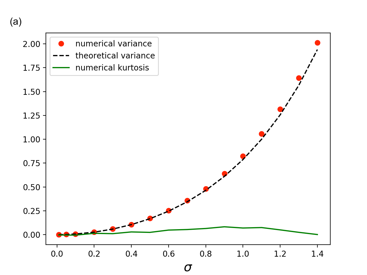
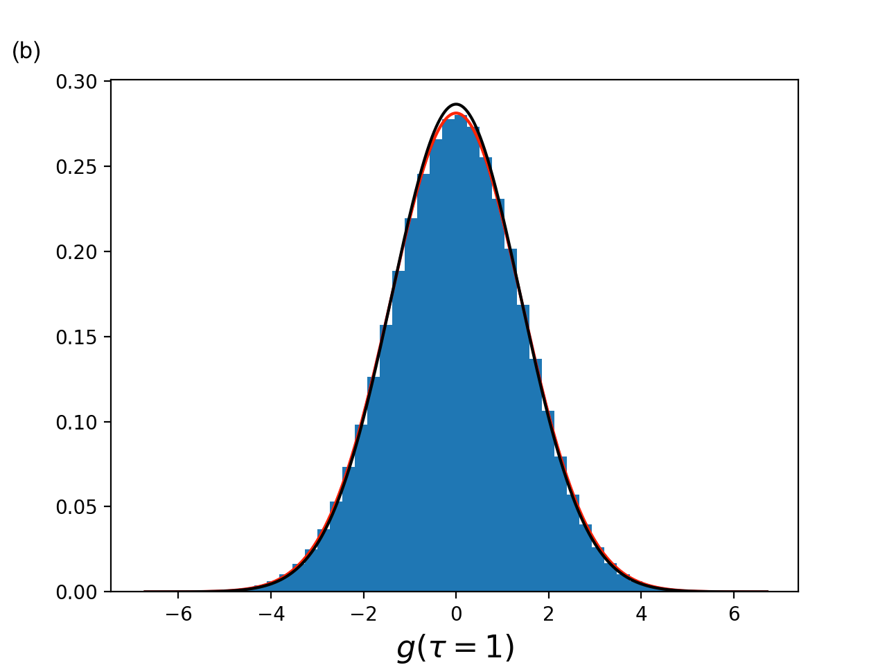
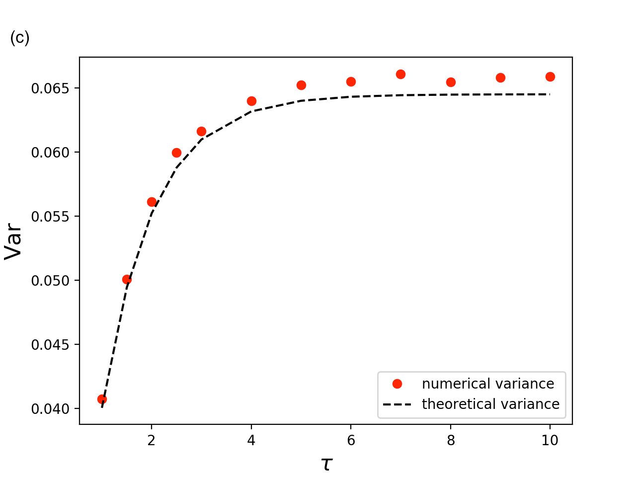
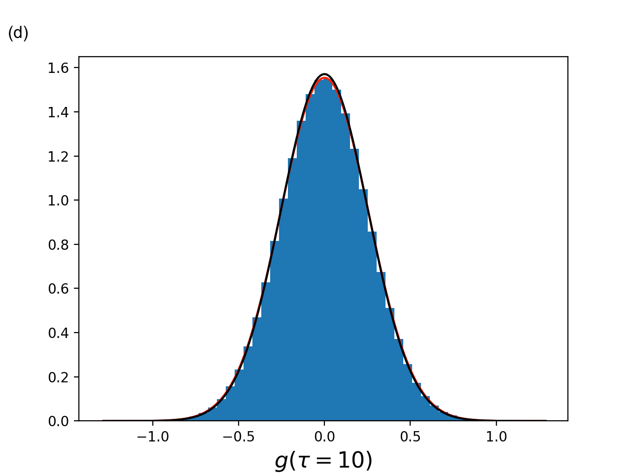
Figure 1: (a) Variance of $P(g,\tau)$ as a function of $\sigma$. Red points are obtained by numerical simulations of the SDE of eq. 5 ($K=1,a=1$). The black dashed line is the analytical approximation of eq. 8. The continuous green line represents the kurtosis of the distributions obtained by the numerical simulations. They are always very close to zero, showing that the distributions have always a Gaussian shape. (b) $P(g,\tau=1)$ for the numerical simulations with $K=1,a=1,\sigma=1.4$. The black line is the distribution obtained by the analytical approximation, the red one is a Gaussian fitting. Note that with these parameters values we are far from the regime where $P(y)$ of eq. 6 is gaussian, nevertheless the approximation continue to work very well. (c) Variance of $P(g,\tau)$ as a function of $\tau$. Red points are obtained by numerical simulations ($K=1,\sigma=0.25$). The black dashed line is the analytical approximation. (d) $P(g,\tau=10)$ for the numerical simulations ($K=1,a=1,\sigma=0.25$). The black line is the analytical approximation, the red one is a Gaussian fitting.

.

4 Results

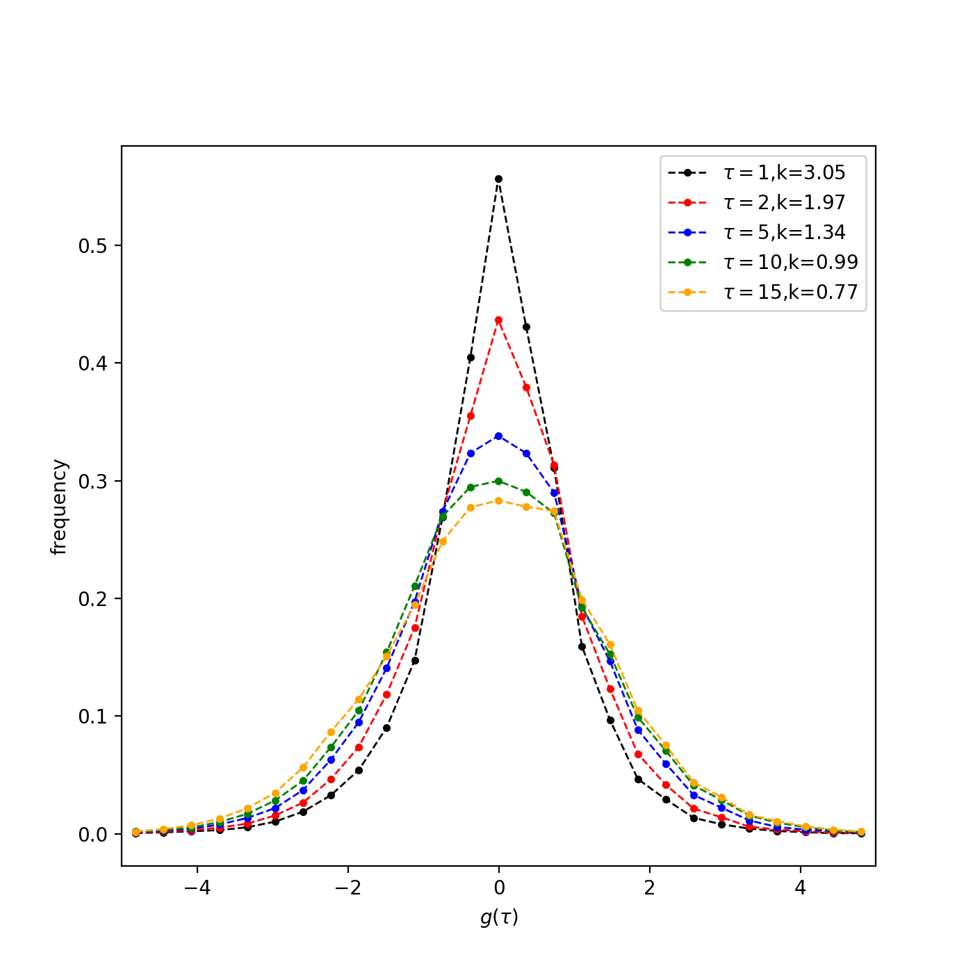
Figure 2: Distribution of log-growth rates measured at different time lags $\tau$. By increasing $\tau$, the distributions present lower peaks but less outliers. This change result in smaller excess kurtosis $k$.

Here we present the study of a selection of the dataset described in section 2 (individual A and individual B). However, similar results are obtained when considering the whole dataset (see Supplementary Material). The first part of the investigation analyzes the ensemble of all time-series present in this selected dataset together, assuming that the same single parametrization of the CIR model is able to describe the population dynamics of all OTUs. Assuming that all OTUs do not strongly interact between each other,we can model them as different realizations of a stochastic process defined by the same parameters. If the neutral hypothesis holds, all species are considered demographically and ecologically equivalent and can be modeled by the same rates.

First, we look at the log-growth rate distributions $P(g,\tau)$ for different values of $\tau$ (see Fig. 2). For small $\tau$ the distributions present a characteristic shape with a sharp and high peak followed by tails that decay slower than a Gaussian distribution. This shape is well characterized by the excess kurtosis ($k=\langle(\frac{x-\mu}{\sigma})^{4}\rangle-3$, where $\mu=\langle x\rangle$ and $\sigma^{2}=\langle(x-\mu)^{2}\rangle$), which is obviously positive and, for $\tau=1$, close to 3. Increasing $\tau$ the excess kurtosis becomes noticeably smaller: peaks decrease and tails become more similar to those of a Gaussian distribution.

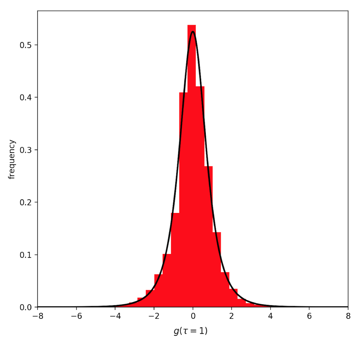
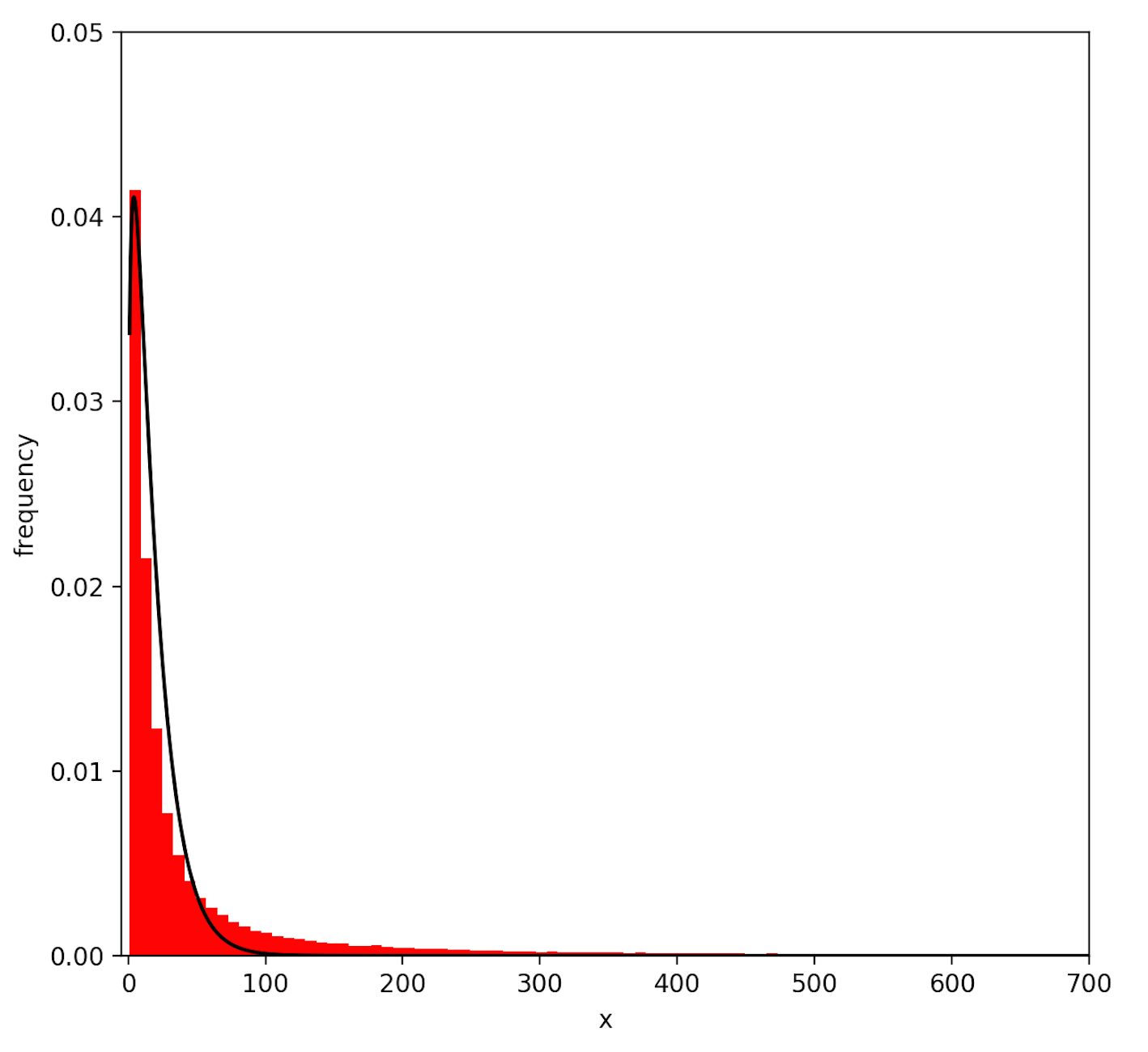
Figure 3: On the left: fit of $P(g,\tau=1)$ using the analytical expression of eq. 3. On the right: the stationary abundance distribution fitted using eq. 2 once fixed $\alpha$ with the results obtained by the estimation of the $P(g,\tau=1)$ parameters.

We focus on $P(g,\tau=1)$ and fit this distribution with eq. 3. Parameters are estimated using the Maximum Log-likelihood method, which provides the values $\alpha=b/D=1.24\pm 0.01$ and $a=3.56\pm 0.02$. The fit is excellent, as can be visually confirmed in Fig.3). To find further support of our hypothesis, we fit abundance experimental data coming from all our time-series with the stationary distribution of eq. 2 once fixed $\alpha$ with the results obtained by the estimation of the $P(g,\tau=1)$ parameters. We obtained $D\cdot a=17.01\pm 0.08$ and a satisfactory fit.

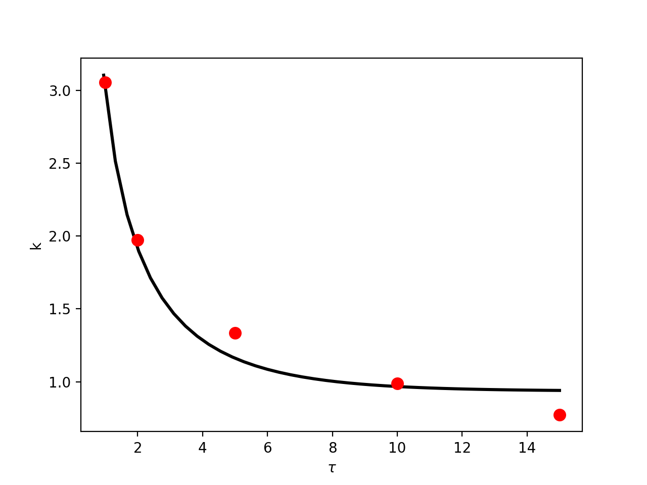
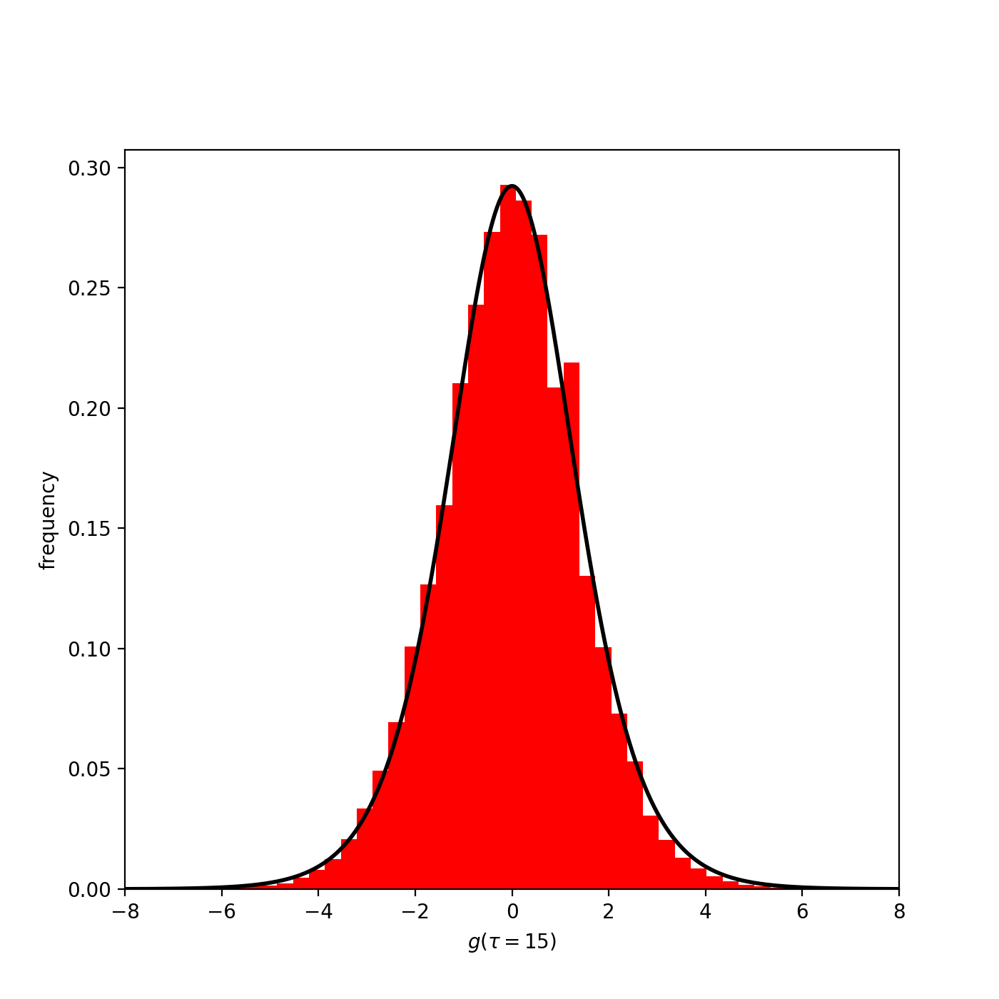
Figure 4: On the left: change of the kurtosis in dependence of $\tau$ values. The continuous line are the values predicted by using eq. 3, using the parameters values estimated at $\tau=1$. Red points are obtained from empirical data. On the right: The analytical distribution for $\tau>>1$ (see eq. 4) using $\alpha$ estimated at $\tau=1$ approximates $P(g,\tau=15)$ obtained from the experimental dataset.

Next, we test how our model can well describe the temporal shift of the shape of the $P(g,\tau)$ towards a distribution with smaller excess kurtosis. We do that by comparing the analytical prediction produced by eq. 3 with our experimental data. Predictions are generated calculating the excess kurtosis at different $\tau$ values from the analytical distribution with the parameters fixed by the estimation at $\tau=1$. Taking into account that kurtosis estimation is very sensitive to outliers, the excess kurtosis obtained from empirical data are very well matched by the analytical prediction, as can be seen in Fig. 4. By using the $\alpha$ value estimated at $\tau=1$ equation 4 can predict the $P(g,\tau)$ for $\tau\to\infty$, which is a very good approximation for every distribution with $\tau>>1$. The remarkably good result is displayed in Fig. 4.

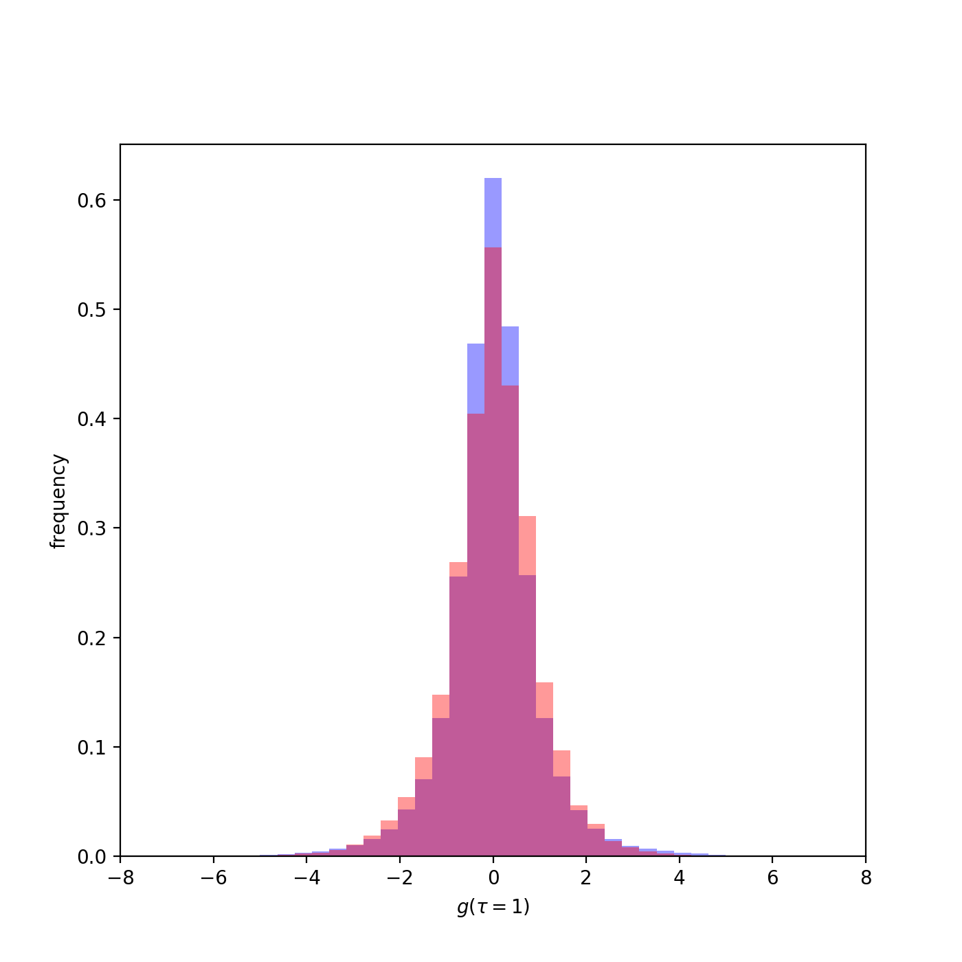
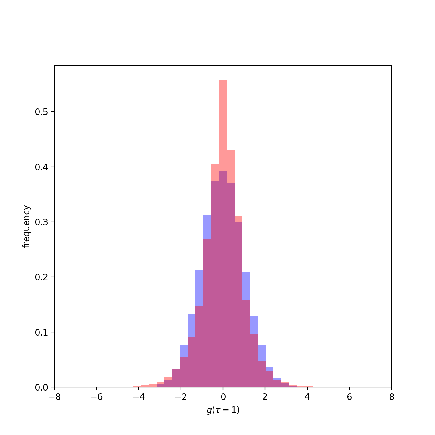
Figure 5: On the left: In red, empirical $P(g,\tau=1)$, in blue the distribution obtained from simulations of the neutral model of eq. 1, calibrated using our scheme based on the log-growth distribution and the stationary abundance distribution. On the right: In red, empirical $P(g,\tau=1)$, in blue the distribution obtained from simulations of the logistic model of eq. 5. The Kolmogorov-Smirnov statistic of the empirical sample with the simulated one is 50% larger than when simulations are performed with the SDE of eq. 1. In this simulation, $\sigma$ and $K$ parameters were calibrated using the stationary distribution, $a$ using $P(g,\tau=1)$ fitted with equation 8 (see Supplementary Material). Note that choosing different values of $a$ does not improve the fit with the empirical data.

Further support to the plausibility of the considered neutral model for describing our dataset can be found by looking at the $P(g,\tau=1)$ produced from long synthetic time-series generated by this model at stationarity. The SDE of equation 1 is calibrated by using the $b/D$ and $a$ values obtained from the log-growth distribution and $D\cdot a$ from the stationary abundance distribution. In Fig. 5 we can see how the synthetic distribution is comparable to the empirical one.

We can perform the same test using the logistic model of equation 5. As can be seen in Fig. 5 synthetic generated data very poorly describe the experimental ones. Even if the distribution of the simulated data generally match the scale of the dispersion of the empirical one, its shape does not adhere to the leptokurtic empirical distribution. This result is in accordance with our prediction of the approximation of eq. 7, which shows that the distribution is always practically indistinguishable from a Gaussian one.

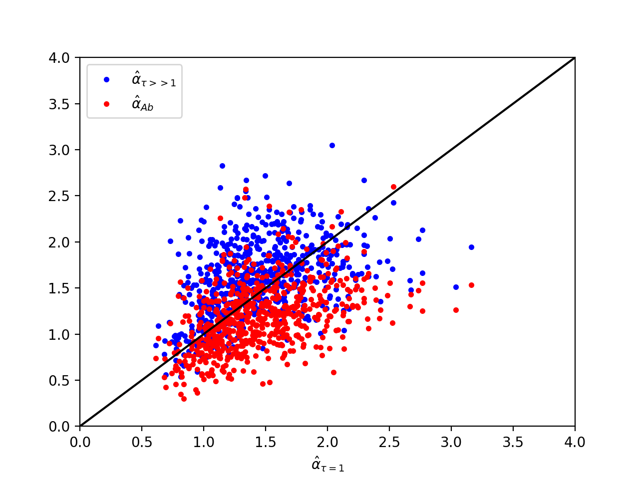
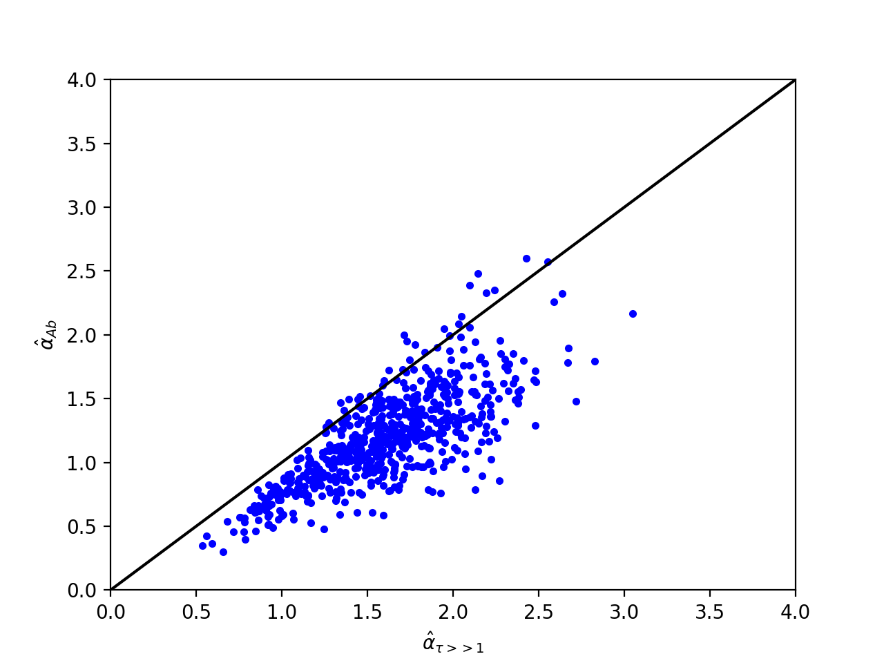
Figure 6: On the left: In this scattering plot blue points represent the $\hat{\alpha}_{\tau=1}$ ($\alpha$ estimated from $P(g,\tau=1)$), versus $\hat{\alpha}_{\tau>>1}$ ($\alpha$ inferred from $P(g,\tau>>1)$). Red points stand for $\hat{\alpha}_{\tau=1}$ versus $\hat{\alpha}_{Ab}$ ($\alpha$ estimated from the stationary abundance distribution). The Pearson correlation is equal to 0.40 and 0.43, respectively. On the right: The scattering plot of $\hat{\alpha}_{\tau>>1}$ versus $\hat{\alpha}_{Ab}$. The Pearson correlation is equal to 0.76. The continuous lines are $x=y$.

Our final evidence supporting the use of the model of eq. 1 comes from the analysis of each time-series taken one by one. In this case we do not assume that they are independent and the parameters that we fit are effective, thus possibly including the effect of interactions. In this approach, we independently fit the log-growth rate distribution for $\tau=1$ (2 fitting parameters), the log-growth rate distribution for $\tau>>1$ (1 fitting parameter) and the stationary abundance distribution (2 fitting parameters). For each time series, we compare the three independently estimated values of $\alpha$, which we indicate as $\hat{\alpha}_{\tau=1}$, $\hat{\alpha}_{\tau>>1}$ and $\hat{\alpha}_{Ab}$. Results can be seen on Fig. 6. Despite the dispersion of the points, which accounts for the heterogeneity of the time series, the estimated values are distributed close to the line $x=y$. Taking into account the size and noise of the time-series, the result suggests that the different approaches used to estimate the parameter values are consistent. A small systematic deviation between $\hat{\alpha}_{\tau>>1}$ and $\hat{\alpha}_{Ab}$ can suggests that the estimated $\hat{\alpha}_{\tau>>1}$ are in general larger than the $\hat{\alpha}_{Ab}$. The results presented in Fig. 6 excluded the time series which generate a $P(g,\tau=1)$ with a shape close to a Gaussian one. These time series are selected for presenting an excess kurtosis of the distribution smaller than $0.5$ and correspond to the $12\%$ of the original dataset. For these data the estimation of $\hat{\alpha}_{\tau=1}$ is not very reliable, and tend to be overestimated in relation to $\hat{\alpha}_{\tau>>1}$ and $\hat{\alpha}_{Ab}$ .

Finally, we report that the mean value of $\hat{\alpha}_{\tau=1}$ is equal to $1.45\pm 0.41$ and the estimation of $a$ coming from the analysis of each time-series taken one by one gives $3.63\pm 2.91$ days. These values are consistent with the ones found by analyzing the ensemble of all time-series together.

5 Discussion

Our results show that the considered neutral model with demographic stochasticity can successfully describe the log-growth rate distributions and the stationary abundance distribution derived from the stationary OTUs abundance time-series. More significantly, the model can predict the temporal dependence of the log-growth rate distribution, by reproducing the kurtosis evolution of $P(g,\tau)$ as a function of $\tau$. Furthermore, the typical shape of $P(g,\tau>>1)$ can be independently assessed using our approach. We can observe that this last distribution generally has a shape that is relatively close to a Gaussian one. It can be hypothesized that weak temporal dependencies between g(t) produce a slight deviation from the convergence to a Gaussian shape, as suggested by aggregational Gaussianity in the case of time additive independent variables. Our analysis reveals another interesting finding: the variance of this distribution does not diverge as $\tau$ increases.

In addition to these results obtained comparing the analytical predictions of the model with the experimental data, we can produce some numerical results which support these outcomes. In fact, the SDE, calibrated with the parameters obtained from the fitting of the distributions, is able to generate simulated processes with a log-growth rate synthetic distribution comparable with the empirical one. Finally, the analysis of each time-series, taken one by one, shows that the parameters inferred by independently fitting the log-growth rate distribution, the same distribution for large $\tau$ and the stationary abundance distribution are consistent. The comparison of their mean values with the estimations derived from the analysis of the ensemble of all time-series together are also consistent. This fact supports a neutral modeling approach: the demographic differences among species are not statistically significant, namely, they can be characterized by the same vital rates in a first approximation.

The most relevant result of our work is the description of the subtle temporal dependence of the log-growth rate distribution. The importance of this result is due to the fact that the distributions that reproduce the abundance and growth rate are flexible enough for describing very different datasets. On varying its parameters, distinct distributions can be seen as a special case of the Gamma one, which can describe data which present shapes close to power-laws, exponential, and even log-normals. The expression of eq. 3 turned out to be really versatile and has been able to reproduce log-growth rate generated by very different systems [26]. These results are important, but not necessarily conclusive for claiming that the considered SDE, with a mean reverting linear drift and demographic noise, can account for the description of so different datasets. Other features or more specific characteristics of the considered distribution, as for example its temporal dependence, should be assessed.

Another important point raised by our analysis is the fact that the logistic model with an environmental stochastic term is not suited for describing the $P(g,\tau)$ found in the considered microbiota dataset at stationarity. This was verified by looking at the distribution generated numerically using this SDE. As a more general conclusion, our analytical results demonstrated that for the regimes with small $\sigma$ this process produces normal $P(g,\tau)$ with a variance dependent on $\sigma$,$a$ and $\tau$. Numerical simulations confirmed that this analytical approximation is good in all the regimes. For these reasons, this approach can not reproduce empirical log-growth rate with leptokurtic distributions, at least in the current formulation. Even if it is difficult to affirm that, considering a linear or a logistic drift term, the presence of a demographic noise is a necessary condition for generating leptokurtic distributions, these results suggest that a simple multiplicative noise is not sufficient.

Finally, our study suggests that neutral models can effectively describe the population dynamics of bacteria in the considered microbiota. The existent literature on this theme reported conflicting evidence. It suggests that human microbial communities are not generally neutral but a small minority of cases already demonstrated the existence of neutral processes [2, 21]. These assessments were generally obtained carrying out an analysis of the characteristic of the community ecology based on macroecological statistical properties. Here, we arrived at this conclusions using a dynamical population approach. In this sense, our results, even if obtained over a limited dataset, are particularly interesting for their implications at the level of biological factors that control the dynamics of the considered populations. In fact, they not only suggest, like every neutral hypothesis, that the selection processes produced by the interactions among the individuals, the species and the environment are relatively less relevant than the demographic stochasticity present in the population dynamics, but also they give a form to the mechanisms that affect population dynamics. Demographic noise seems to be relatively more important than the environmental one for explaining $P(g,\tau)$. Stochastic logistic models with quenched noise (e.g., random parameters) can provide a wider variability in the temporal evolution of the population size and therefore an improved explanatory power which might better describe log-growth distributions. However, this approach is outside the scope of the present work.

6 Acknowledgments

E.B. thanks the LIPh lab at the Departamento di Fisica of the Università di Padova for its hospitality during the realization of this work. The authors acknowledge Jacopo Pasqualini for pre-processing the dataset considered in this analysis and Amos Maritan, Emanuele Pigani and Samir Suweis for fruitful discussions.

E.B. received partial financial support from the National Council for Scientific and Technological Development - CNPq (Grant No. 305008/2021-8).

References

References

- [1] Faust, K., Lahti, L., Gonze, D., de Vos, W. M., Raes, J. Metagenomics meets time series analysis: unraveling microbial community dynamics. Curr. Opin. Microbiol. 25, 56-66 (2015).
- [2] Li, L., Ma, Z. S. Testing the neutral theory of biodiversity with human microbiome datasets. Sci. Rep. 6, 31448 (2016).
- [3] Shoemaker, W. R., Locey, K. J., Lennon, J. T. A macroecological theory of microbial biodiversity. Nat. Ecol. Evol. 1, 107 (2017).
- [4] J. Grilli, Macroecological laws describe variation and diversity in microbial communities. Nat. Commun. 11, 4743 (2020).
- [5] David, L. A. et al. Host lifestyle affects human microbiota on daily timescales. Genome Biol. 15, R89 (2014).
- [6] Royama, T. Analytical Population Dynamics (Chapman & Hall, London, 1992).
- [7] Berryman, A., Turchin, P. Identifying the density-dependent structure underlying ecological time series. Oikos 92, 265-270 (2001).
- [8] Brigatti E, Vieira MV, Kajin M, Almeida PJ, de Menezes MA, Cerqueira R. Detecting and modelling delayed density-dependence in abundance time series of a small mammal (Didelphis aurita). Sci Rep. 2016 Feb 11;6:19553.
- [9] Ji, B.W., Sheth, R.U., Dixit, P.D. et al. Macroecological dynamics of gut microbiota. Nat Microbiol 5, 768-775 (2020).
- [10] Keitt, T. H. and Stanley, H. E. Dynamics of North American breeding bird populations. Nature 393, 257-260 (1998).
- [11] Stanley, M. H. R. et al. Scaling behaviour in the growth of companies. Nature 379, 804-806 (1996).
- [12] Dosi, Giovanni. 2005, Statistical regularities in the evolution of industries. a guide through some evidence and challenges for the theory, LEM Papers Series 2005/17, Lab- oratory of Economics and Management (LEM), Sant’Anna School of Advanced Studies, Pisa, Italy. Available at http://ideas.repec.org/p/ssa/lemwps/2005-17.html.
- [13] Y. Schwarzkopf and J. D. Farmer, Time Evolution of The Mutual Fund Size Distribution, Santa Fe Institute Working Paper, 08-08-031, (2008).
- [14] Luiz G.A. Alves, Haroldo V. Ribeiro, Renio S. Mendes, Scaling laws in the dynamics of crime growth rate, Physica A, 392, 2672-2679, (2013).
- [15] R. Cont (2001) Empirical properties of asset returns: stylized facts and statistical issues, Quantitative Finance, 1:2, 223-236.
- [16] De Sousa Filho FNM, Silva JN, Bertella MA, Brigatti E. 2021 The leverage effect and other stylized facts displayed by Bitcoin returns. Braz. J. Phys. 51, 576-586.
- [17] Azaele S, Pigolotti S, Banavar J, Maritan A. 2006 Dynamical evolution of ecosystems. Nature 444, 926-928.
- [18] Hubbell SP. 2001 The unified neutral theory of biodiversity and biogeography. Princeton, NJ: Princeton Univ. Press.
- [19] Volkov I, Banavar JR, Hubbell SP, Maritan A. 2003 Neutral theory and relative species abundance in ecology. Nature 424, 1035-1037.
- [20] S. Azaele et al., Rev. Mod. Phys., 88, 035003 (2016); F. Peruzzo et al., Phys. Rev. X, 10, 011032 (2020); S. Azaele et al., Phys. Rev. E, 80, 031916 (2009).
- [21] L. Descheemaeker S. de Buyl (2020) Stochastic logistic models reproduce experimental time series of microbial communities, eLife 9:e55650.
- [22] S. Zaoli, J. Grilli (2021) A macroecological description of alternative stable states reproduces intra- and inter-host variability of gut microbiome, Sci. Adv., 7, eabj2882.
- [23] J. G. Caporaso, C. L. Lauber, E. K. Costello, D. Berg-Lyons, A. Gonzalez, J. Stombaugh, D. Knights, P. Gajer, J. Ravel, N. Fierer, J. I. Gordon, R. Knight, Moving pictures of the human microbiome. Genome Biol. 12, R50 (2011).
- [24] Feller, W. (1951) Two singular diffusion problems, Ann. of Math., 54(1), 173-182.
- [25] Cox, J.C., Ingersoll, J.E., Ross, S.A. (1985) A theory of the term structure of interest rates, Econometrica, 53, 385-408.
- [26] Ashish B. George, James O’Dwyer, Universal abundance fluctuations across microbial communities, tropical forests, and urban populations, arXiv:2209.07628 (2023).