Graph Neural Networks for Pressure Estimation in Water Distribution Systems

Abstract

Pressure and flow estimation in Water Distribution Networks (WDN) allows water management companies to optimize their control operations. For many years, mathematical simulation tools have been the most common approach to reconstructing an estimate of the WDN hydraulics. However, pure physics-based simulations involve several challenges, e.g. partially observable data, high uncertainty, and extensive manual configuration. Thus, data-driven approaches have gained traction to overcome such limitations. In this work, we combine physics-based modeling and Graph Neural Networks (GNN), a data-driven approach, to address the pressure estimation problem. First, we propose a new data generation method using a mathematical simulation but not considering temporal patterns and including some control parameters that remain untouched in previous works; this contributes to a more diverse training data. Second, our training strategy relies on random sensor placement making our GNN-based estimation model robust to unexpected sensor location changes. Third, a realistic evaluation protocol considers real temporal patterns and additionally injects the uncertainties intrinsic to real-world scenarios. Finally, a multi-graph pre-training strategy allows the model to be reused for pressure estimation in unseen target WDNs. Our GNN-based model estimates the pressure of a large-scale WDN in The Netherlands with a MAE of 1.94mH₂O and a MAPE of 7%, surpassing the performance of previous studies. Likewise, it outperformed previous approaches on other WDN benchmarks, showing a reduction of absolute error up to approximately 52% in the best cases.

Keywords Graph Neural Networks  $\cdot$ Water Distribution Networks  $\cdot$ Pressure Estimation  $\cdot$ State Estimation  $\cdot$ GNN  $\cdot$ WDN

1 Introduction

State Estimation in Water Distribution Networks (WDNs) is a general problem that encompasses pressure and flow estimation, often using scarce and sparsely located sensor devices. WDNs management companies rely on such estimations for optimizing their operations. Knowing the state of the network at any given time enables water managers to perform real-time monitoring and control operations. The research community and practitioners working in this field have resorted for many years to the power of mathematical simulation tools to reconstruct an estimate of the system hydraulics (Fu et al., 2022a, ; Garzón et al.,, 2022). However, pure physics-based simulation approaches have to overcome the challenges of (i) data scarcity which translates to partially observable systems, (ii) high uncertainty introduced by the large number of parameters to configure, unexpected changes in consumers’ behavior reflected in uncertain demand patterns, and noisy sensor measurements, and (iii) extensive manual configuration that requires expert knowledge and usually hinders model re-usability in a different WDN (Wang et al.,, 2021; Fu et al., 2022a, ). The challenges associated with physics-based modeling of WDNs have motivated researchers to investigate the usage of data-driven approaches, or a combination of both, to address the state estimation problem (Meirelles et al.,, 2017; Lima et al.,, 2018).

Graph Neural Networks (GNNs) is a data-driven approach that has shown successful results in several estimation problems where data lies outside the Euclidean domain, and can be modeled as a graph. Since WDNs can be naturally modeled as a graph, GNNs can exploit the relational inductive biases imposed by the graph topology. As a result, GNNs have also attracted the attention of researchers in the field of WDNs. For example, (Tsiami and Makropoulos,, 2021) used temporal graph convolutional neural networks, a combination of Convolutional Neural Networks (CNNs) and GNNs, to extract temporal and spatial features simultaneously in a model to detect cyber-physical attacks in WDNs. (Zanfei et al.,, 2022) leveraged GNNs for burst detection algorithms. GNNs are also used for integrated water network partitioning and dynamic district metered areas (Fu et al., 2022b, ). In the context of Digital Twins of WDNs, a GNN-based model is used for Pump Speed-Based State Estimation (Bonilla et al.,, 2022). Other works are more similar to ours and use GNNs for pressure estimation (Hajgató et al.,, 2021; Ashraf et al.,, 2023).

In this work, we focus on pressure estimation by leveraging both physics-based simulation models and GNN-based data-driven approaches. Our work proposes a number of research contributions. First, we propose an advanced data generation model to overcome the lack of data required for model training. Our method relies on a mathematical simulation tool, but it does not consider time-dependent patterns, producing a more diverse training dataset. In addition, we include some control parameters that remain untouched in previous works which contributes to data variety and avoids that uncertainties propagate due to model simplification errors (Du et al.,, 2018). Second, our GNN-based estimation model is robust to unexpected sensor’s location changes due to the proposed training strategy that relies on random sensor placement. Third, we propose a realistic evaluation protocol. Thus, our test set generation method considers real time-dependent patterns and additionally injects the uncertainties intrinsic to real-world scenarios. Finally, the proposed GNN-based model is equipped with generalization capabilities by design, and a multi-graph pre-training strategy allows to reuse the model for pressure reconstruction in different WDNs.

As a consequence, our model reconstructed the junction pressures of Oosterbeek, a large-scale WDN in the Netherlands, with an average 1.94mH₂O absolute error, which represents an 8.57% improvement with respect to other models. Similarly, our model outperformed previous approaches on other WDNs benchmark datasets. The highest improvement was seen for C-Town (Ostfeld et al.,, 2012) with an absolute error decrease of 52.36%, for Richmond (Van Zyl,, 2001) an error deacrease of 5.31%, and 40.35% error decrease for L-Town (Vrachimis et al.,, 2022). In addition, our first attempt on model generalization shows that a multi-graph pre-training followed by fine-tuning helps to increase the model performance. In our case, the absolute error on Oosterbeek network reduced from 1.94 to 1.91mH₂O following our generalization strategy.

The remainder of this document is as follows. Section 2.3 describes the issues that need to be addressed by pressure reconstruction models and defines the criteria to assess the model capabilities. Section 3 depicts the related work in the field, narrowed to GNNs for node-level regression tasks and how previous work on GNN-based pressure estimation satisfies the criteria defined in the Section 2.3. The methodology is presented in Section 4, including the data generation process, a detailed description of our model architecture, and the details of the proposed approach for model training and evaluation. Section 5 describes the setup of the experimental phase. It includes a description of WDNs benchmark datasets used in this work, the base model configurations, and the evaluation metrics. Section 6 describes all the empirical evaluations of our approach. First, the experiments on the main use case of this study, Oosterbeek WDN, are depicted. Then, the experiments towards model generalization are shown. Next, the performance of the proposed model on different benchmark WDNs is presented. This section concludes with an ablation study to identify the contribution of the different components of the model architecture. A discussion of the most salient findings are presented in Section 7. Finally, the conclusions are presented in Section 8.

2 Pressure estimation in water distribution networks

2.1 Problem statement

Hydraulic experts have managed water distribution networks using essential measurements such as flow, demand, and pressure. These measurements offer a comprehensive perspective of a water distribution network, forming a foundation for various supervisory tasks like forecasting, leak detection, and operational control. In this study, we narrowed down our work to estimate pressure due to the ease of meter installation and the more affordable price compared to flow ones (Zhou et al.,, 2019). Nevertheless, to approximate a complete view of pressure in different locations in the water network, we use a data-driven model that can confront existing issues in practical water distribution networks.

A real-life water network can include thousands of junctions indicating water outlets, customers, and pipe interactions. However, only some junctions are sensor-equipped and well-maintained due to infrastructural limits and privacy concerns. Thus, they raise the need for more data and observable sensors to train a pressure estimation model in a high-quality manner. Specifically, during training, the model – typically structured with deep learning architectures as its backbone – learns to estimate the pressure at all unknown junctions within the network, relying on measurements from only a limited number of sensors. This approach recalls a typical semi-supervised learning problem with more considerations in the deployment context.

The application context is about what and when the trained model should be applied. Generally, a model is often associated with a unique water network and fixed sensors previously seen during training. Also, the training environment may exclude noisy, uncertain conditions that could affect the model’s decision-making. In other words, these challenges result in worse model performance when faced with unfamiliar network topologies or uncertain situations. Consequently, model retraining is inevitable, albeit such training is an expensive and unsustainable approach. This concern enhances the necessity of the generalization ability of pressure estimation models, which needs to be addressed in prior research. Before addressing this research gap, we will first delve into the specific problem within water networks and lay out the criteria necessary for a robust pressure estimation model.

2.2 Partially-Observable Data and Realistic Model Evaluation

Water Distribution Networks domain is characterized by partial-observability due to the limited sensor coverage. This imposes an additional challenge because the reconstruction models need to be trained on fully-observable network operation snapshots. The common approach to overcome this limitation is to rely on mathematical hydraulic simulation tools, e.g. EPANET (Rossman,, 1999), WNTR (Klise et al.,, 2018), to generate full-views of the network operation and use them for model training (Hajgató et al.,, 2021; Xing and Sela,, 2022; Ashraf et al.,, 2023; Zhou et al.,, 2023).

Although the hydraulic simulations solve the lack of training data for the reconstruction models, the remaining challenge is how to create a valid and reliable evaluation protocol and the data used for it. Sampling from the data generated from the simulation models and splitting them into training and test sets is not enough. Ideally, the assumption behind machine learning models is that the training data is ruled by the exact same distribution of the data on which the model will be evaluated. However, having absolute control over the data generation process and meeting such a perfect match between both distributions is unrealistic and the assumption is violated under real-world conditions (Bickel et al.,, 2007; Hendrycks and Gimpel,, 2017; Fang et al.,, 2022). Thus, the prediction models should be robust to distribution shifts between training and testing samples, i.e., be able to generalize to out-of-distribution (OOD) data (Farquhar and Gal,, 2022).

Figure 1: Density Distribution of training and test sets in C-Town, Richmond, L-Town and Oosterbeek WDNs, generated by the Hydraulic Simulation tool EPANET.

We observed that the data distribution of the training and test sets created by the simulation models are identical, which is unnatural in practice. The density distributions of training and test sets from different WDNs, generated by the Hydraulic Simulation tool EPANET, are shown in Figure 1. In this case, the simulation’s control parameters, e.g. reservoir total heads, junction demands, pump speed, were randomly adjusted for every run. Nonetheless, as evident from the image, the distributions of the training and test sets created by the hydraulic simulations are identical in all examples. In this case, evaluating the reconstruction models on data generated by the same algorithm is simply evaluating the ability of the model to reconstruct the signals already seen during the training process.

In our work we propose a realistic test set generation process that relies on time-based demand patterns. In addition, Gaussian noise is injected before the simulation to mimic the uncertainty intrinsic to real-world scenarios. Combining time-based demand patterns and noise injection allows to create realistic scenarios to evaluate the ability of the models to generalize to OOD data, with visible differences in density distribution between training and test sets.

2.3 Criteria for model assessment

The out-of-distribution problem is a persistent challenge in mathematical simulations, originating from uncertainty and variability in hydraulic parameters, such as consumer demand, pipe roughness, and material aging attributes. Modeling and monitoring these values are complex and costly. This difficulty arises exponentially in sophisticated cases, such as fluids in curved pipes, lack of measurements, or when exterior reasons cause unforeseen effects on the network (Campos et al.,, 2021). In addition, the generalization ability is weak because the hydraulic simulations cannot be applied to an unseen water network. Thus, they cannot deal with such problems and lag behind their standard capability.

In light of the limitations of conventional simulations, previous studies have proposed using more efficient surrogate models (which we will discuss in Section 3). However, it is critical to note that they overlooked the OOD problem. Thus, it essentially motivates a list of criteria that indicate the favorable capabilities of a surrogate model addressing the pressure estimation task on water distribution networks while taking into account the OOD, generalizability, and flexibility as follows.

1. $\bm{(\mathbb{C}1)}$ The surrogate model should have topology awareness to effectively solve the pressure estimation task. In addition, it must be able to perform seamlessly on any Water Distribution Network, regardless of whether its topology is observable during training. This is an important aspect of generalizability, making it more useful in practice.

2. $\bm{(\mathbb{C}2)}$ The surrogate model should be adaptable to various contextual circumstances. Adjusting a variety of sensor measurements can be a typical example. This criterion allows for model flexibility when new measurement meters are introduced. In addition, it counters situations where one or more sensors are deactivated for maintenance purposes.

3. $\bm{(\mathbb{C}3)}$ To capture the OOD problem, model robustness should be taken into account, especially in the evaluation phase. The uncertainty inherited from the real world can yield noise in observations, including data transmission and discrepancy of hydraulic parameters between simulated and actual water networks. Many existing approaches do not address these issues, as they are often tested in well-simulated and noise-free cases that do not account for uncertainty.

Satisfying all factors simultaneously is difficult. For this reason, the provided list is used to evaluate the state-of-the-art methods for estimating pressure in the next section. Then, we will introduce our solution that fulfills all three criteria on the list. Our empirical experiments have shown that the suggested model outperforms other baselines, even when taking into account its parameter complexity.

3 Related Work

3.1 GNNs for node-level regression task

(Wu et al.,, 2021) categorized GNN based on their purposes into graph-level, link-level, and node-level tasks. These categories indicate the versatility and primary focus of GNN to provide outcomes across various domains. For instance, graph-level and link-level have been employed in domains such as chemistry (Reiser et al.,, 2022), bioinformatics (Nguyen et al.,, 2020), and recommendation systems (Chen et al., 2020c, ). On the other hand, the node-level category has been dominated by node classification tasks. One illustrative example is in the field of physics, where GNN can predict the probability that an individual particle is associated with the pileup part of an event(Shlomi et al.,, 2020). In finance, loan fraud detection within consumer networks is a popular example of a node classification task (Xu et al.,, 2021).

As an influence of prevalent node classification tasks, well-known GNN architectures have been developed to excel in this domain (Defferrard et al.,, 2016; Chen et al., 2020b, ; Veličković et al.,, 2018). This focus led to a relative lack of attention in node regression tasks and caused ambiguity regarding their effectiveness in handling continuous values within the node-level regime. Hence, in this paper, we aim to bridge the research gap and explore the potential of these methods in addressing node regression challenges.

While some studies have started exploring node-level regression in specific domains, such as traffic (Derrow-Pinion et al., 2021a, ) and recommendation systems (Ying et al.,, 2018), the water domain remains relatively unexplored. With this in mind, our primary objective is to compare popular approaches in a regression task known as pressure estimation and to introduce our cutting-edge GNN architecture designed for this purpose. It could open new avenues for GNN applications, especially in water management.

3.2 State Estimation with GNNs

State Estimation plays a critical role as a fundamental process that provides adequate information for WDN management, monitoring, and maintenance, such as leak localization (Mücke et al.,, 2023), optimal control (Martínez et al.,, 2007) and cyber-attack detection (Taormina et al.,, 2018). Recent works have started to study GNNs when they outperformed classical models in graph-related tasks, especially in pressure estimation (Hajgató et al.,, 2021). Generally, GNN attempts to predict all pressure values at nodes using limited historical sensor values. For an overview, we list the most important works and evaluate them against the predefined criteria.

(Hajgató et al.,, 2021) is the first work that proposes to train a GNN model named ChebNet on a well-defined synthetic dataset. $\bm{(\mathbb{C}2)}$ are satisfied because the authors trained the model on various snapshots concerning different sensor locations. In contrast, achieving $\bm{(\mathbb{C}3)}$ is vague as all reports were based on time-irrelevant and synthetic data. In addition, the model cannot deal with the generalization problem due to the limitation of spectral-based models (Zhang et al.,, 2019). Concretely, each spectral model is trained on and linked to a particular topology, so using a single model on diverse WDNs is impractical. Hence, it fails to satisfy $\bm{(\mathbb{C}1)}$.

(Ashraf et al.,, 2023) improved the above work on historical data. In this case, working with a spatial-based GNN can solve the generalization problem, so it is possible to satisfy $\bm{(\mathbb{C}1)}$. In addition, testing on noisy time-relevant data could be seen as an uncertainty consideration . However, this work heavily depends on historical data generated from a pure mathematical simulation engaging with “unchanged" dynamic parameters (e.g., customer demand patterns). In practice, this approach does not apply to the cases where those parameters are prone to error or unknown (Kumar et al.,, 2008). Hence, we consider that it weakly satisfies $\bm{(\mathbb{C}3)}$. However, the author fixed sensor positions during training, which could negatively affect the model observability to other regions in the WDN. For this reason, stacking very deep layers that increase model complexity is inevitable to ensure the information propagation from far-away neighbors to fixed sensors (Barceló et al.,, 2020). Additionally, retraining the model is mandatory whenever a new measurement is introduced, which has detrimental effects on its flexibility and scalability. Thus, the model violates $\bm{(\mathbb{C}2)}$.

Note that we exclude the heuristic-based methods as they do not consider the topology in decision-making. Also, several graph-related approaches (Kumar et al.,, 2008; Xing and Sela,, 2022) have existed in this field. However, they accessed historical data, and neither attempted to solve the task in a generalized manner. Alternatively, we assume that prior knowledge (i.e., historical data) is unavailable. In this work, we delve into the capability of GNNs in a general case, in which the trained model can be applied to any WDN and any scenario.

4 Methodology

4.1 Water network as graph

A water distribution network is a complex infrastructure that provides safe and reliable access to clean water for individual usage. Thus, it is crucial to ensure it properly functions and sustainably meets the needs of the serving community. This monitoring process starts with gathering information from data streams captured by sensors installed in the network. For notation, we define a finite segment of the data stream as a scenario. Each scenario is divided into snaphots, preserving the network state at a particular timestamp.

Mathematically, a snapshot is represented as a finite, homogeneous, and undirected graph $\mathcal{G}=\{\mathcal{X},\mathcal{E},\mathcal{A}\}$ that has $N$ nodes and $M$ edges. Edges represent pipes, valves, and pumps, while nodes can be junctions, reservoirs, and tanks. The nodal features are stored in the matrix $\mathcal{X}\in\mathbb{R}^{N\times d_{node}}$, where $|\mathcal{X}|=N$ and $d_{node}$ is the number of feature channels. In this work, pressure is the unique node feature because it is recognized as the most vital stable factor in monitoring the WDN (Christodoulou et al.,, 2018) and aligns with prior research(Hajgató et al.,, 2021; Ashraf et al.,, 2023). Thus, from now, we refer $\mathcal{X}$ to a pressure matrix, and the feature dimension $d_{node}$ is fixed to 1.

$\mathcal{E}\in\mathbb{R}^{M\times d_{edge}}$ is an edge feature matrix, where $|\mathcal{E}|=M$ and $d_{edge}$ is the edge dimension. Depending on a particular model, we set $d_{edge}$ to $0$ if unused or $2$, which indicates pipe lengths and diameters are supported. The node connection is represented in an adjacency matrix $\mathcal{A}\in\mathbb{R}^{N\times N}$, where $a_{ij}=1$ means node $i$ and $j$ are connected by a link, whose edge attribute $e_{ij}\in\mathcal{E}$, and $a_{ij}=0$ for otherwise.

Observing accurate pressure $\mathcal{X}$ for an entire water network is challenging due to partial observability. Hence, we rely on a physics-based simulation model to construct synthetic pressure as training samples for the surrogate model. Concretely, the simulation takes a range of simulation parameters, including static parameters, such as nodal elevation and pipe diameter, and dynamic parameters, like junction demands and tank settings. Then, it solves a hydraulic equation to estimate the pressure and flow at unknown nodes in a Water Distribution Network (Simpson and Elhay,, 2011). Note that in our case, as we tackle a multi-topology problem, we flexibly compute head losses modeled in pipes using various formulas, such as Hanze-Williams, Daisy-Wechbach, and Chezy-Manning. For more details on solving hydraulic optimization, we refer the reader to the EPANET engine, which serves as our default mathematical simulation (Rossman,, 1999).

Despite the usability of conventional simulations, they demand a manual calibration process to stay synchronized with the actual physical water network. Also, they lack efficiency and suffer from the OOD problem mentioned in Section 2.3. In light of these limitations, we adopt a strategic alternative. In particular, we merely leverage a simulation model to generate synthetic samples once. Subsequently, these synthetic samples serve as the training data for our calibration-free surrogate model. The trained model can infer the pressure of any water network in the deployment. In the following section, we focus on the first stage, where we construct the training dataset using the conventional simulation.

4.2 Dataset creation

Throughout this paper, GNNs take WDN snapshots as input features. In particular, each snapshot provides a global view of a WDN graph representing concrete pressure values at an arbitrary time. Additionally, it contains topological information (e.g., nodal degree, node connectivity, and edge attributes) from a corresponding water network. We denote as a clean snapshot the one that describes an instantaneous pressure state without any hidden information. In contrast, a masked snapshot portrays a partially observable network in which the target feature known as pressure is mostly undetermined except for a small number of metered areas.

The conventional generation requires temporal patterns to create a set of clean snapshots. A pattern records a time series of a specific simulation parameter, such as customer demand or pump curve, in a fixed period. In other words, such a series is periodic and bound in common scenarios. However, it is not guaranteed that these patterns include all events, and real-world data is highly volatile. For example, a model trained on data created from past patterns can fail to estimate the pressure of a WDN during the long-term COVID-19 pandemic due to the unexpected sudden change in water consumption that was never found in such patterns (Campos et al.,, 2021). Furthermore, the number of available patterns is seldom provided or partially accessible due to privacy-related concerns, especially in public benchmark WDNs. For this reason, they are often repetitively overused in modeling large-scale water networks where the number of nodes is exponential compared to the required patterns. This significantly impacts dataset diversity and, therefore, limits the model capability to satisfy criteria $\bm{(\mathbb{C}3)}$.

Before proposing our alternative solution, we review existing generation methods to analyze the effect of time-series patterns on simulation parameters. Generally, two existing options include time-dependent and sampling-based ones. Table 4.2 indicates the existing methods for selecting and altering dynamic parameters. The underlying simulation still plays a crucial role in creating clean snapshots given an arbitrary set of parameters. Still, each method has a specific selection and adjustment of dynamic parameters with respect to a design space.

Table 1: The selection of dynamic parameters between conventional simulations and sampling-based generations. Parameters marked with a check can exhibit varying values, whereas others remain constant throughout the generation process. Note that the dynamic parameter selection also depends on component availability in a particular network and dataset creation stability to prevent abnormal results.

1.5cmDataset Creation	1.4cmReservoir Total Heads	1.3cmJunction
Demand	1.4cmPump
Speed	1.4cmPump
Status	1.4cmTank
Levels	1.4cmValve
Settings	1.4cmValve
Status	1.4cmPipe
Roughness
(Rossman,, 1999)	✓	✓	✓a
(Hajgató et al.,, 2020)		✓	✓	✓	✓
Our	✓	✓	✓	✓	✓	✓	✓	✓
a Pump speed is implicitly adjusted by a pump curve pattern.

The conventional simulation method, EPANET (Rossman,, 1999), operates time-dependently and relies primarily on fixed patterns. Excessive use of these patterns results in temporal correlations among snapshots, primarily due to their inherent seasonal factors. This issue becomes inevitable, especially in large-scale networks, where numerous unmeasurable nodes require pattern assignments to complete a simulation process. Consequently, this leads to information leakage between snapshots within the same scenario (see after-splitting data distribution in training and testing sets in Figure 1).

Alternatively, (Hajgató et al.,, 2020) eliminate time patterns and consider a single snapshot as an instantaneous scenario. This way is more delicate to provide more observations for data-hungry models. However, (Hajgató et al.,, 2020) focus only on pump optimization, so half of the listed parameters remain untouched.

Both available generations assume the remaining parameters are deterministic and unchanged. Nevertheless, these parameters (e.g., pipe roughness) can be critical factors affecting the simulation result (Zanfei et al.,, 2023). Thus, neglecting any of these parameters can restrict the model in learning representations of WDN snapshots.

Intuitively, we consider a comprehensive modification of all dynamic parameters as a data augmentation to ensure the simulation quality and address the generalization problem. Our main objective is to design a sufficient search space to provide different pressure views from flexible sensor positions. This approach helps alleviate the data-hungry issue when training deep learning models and benefits model robustness thanks to the augmented data space (Cubuk et al.,, 2020).

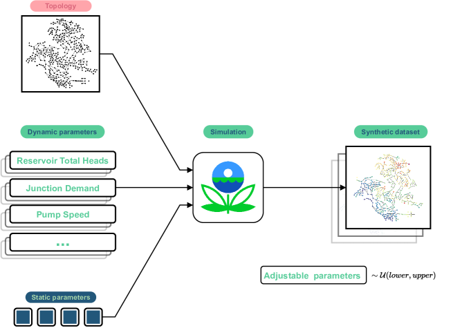
Figure 2: Our data generation approach. Dynamic parameters are sampled from a uniform distribution and passed to the mathematical simulation with static values and WDN topology. The result is a synthetic dataset containing legit snapshots whose pressure range should be close to reality.

In particular, we adopt a brute-force approach to explore the full range of available dynamic parameters. To ensure the simulation quality, we exclude parameter sets producing pressure ranges exceeding practical limits. Subsequently, our generation takes these sets of dynamic parameters, an unchanged static set, and the topology of a particular water network to generate a single snapshot using the conventional simulation (refer to Figure 2). Note that it only performs a single simulation step that removes the essence of temporal patterns. This process outcome is a set of distinct immediate pressure states, which are more versatile and independent in time. In contrast to the classical usage, this approach eliminates the temporal correlation concern and leverages all dynamic parameters to generate training samples designed to cover the entire input space.

4.3 Model Architecture

The model is expected to learn a graph representation from existing known signals to estimate unknown pressures. After this, given a deterministic topology, we need an approach to spread local representations from meter nodes to distant neighbors efficiently. We first recap Message Passing Neural Networks (MPNN) (Gilmer et al.,, 2017), the generic framework for spatial GNNs. Then, we discuss Graph Attention Network (GAT) (Veličković et al.,, 2018) as one of our fundamental components. In light of this, we propose GATRes as a principal block and devise the overall architecture illustrated in Figure 3.

4.3.1 Preliminaries

Considering a GNN as a series of stacked layers, MPNN describes a specific layer to transform previous representations to successive ones using message propagation. We omit the layer index for simplicity and denote representations of a target node $i$ as $x_{i}$. Noticeably, the first representations are input features known as pressure values. Then, the output representations of a consecutive layer are computed as follows:

$$z_{i}=\textrm{UPDATE}\left(x_{i},\bigoplus_{j\in\mathcal{N}(i)}\textrm{MSG}(x_{j})\right)$$ (1)

where $z_{i}$ is the corresponding output of the target node $i$, $\mathcal{N}(i)$ denotes the 1-hop neighbors, MSG and UPDATE are differential functions describing messages received from neighbors and the way to update that information concerning its previous representations respectively.

$\bigoplus$ is a differentiable, permutation-invariant function, ensuring the gradient flow backward for model optimization and addressing concerns related to node ordering (Gilmer et al.,, 2017). This function plays a critical role in aggregating neighbor messages into the target one.

Depending on the task-specific purpose, numerous ways exist to define the message aggregator, such as mean, max, sum (Xu et al.,, 2019), or Multilayer Perceptron (Zeng et al.,, 2020). Ideally, $\bigoplus$ is designed to propagate messages from surrounding nodes in a sparse fashion, which only matters to non-zero values. Thus, this scheme efficiently scales when dealing with enormous graphs and economically saves the memory allocation budget.

Next, we explain GAT in view of a target node $i$. Concretely, GAT focuses on the intermediate representation relationship between the target node $i$ and one of its 1-hop neighbors $j$. If a node pairs with itself, it forms a self-attention relationship. Hence, we strategically establish a virtual self-loop link in every node to put weights between itself representations compared to the aggregated ones from the neighborhood. Mathematically, we can rewrite the GAT formula according to Equation 1 as:

$$z_{i}=\overset{H}{\underset{h}{\bigg{|}\bigg{|}}}\underset{j\in\mathcal{N}(i)\cup\{i\}}{{\sum}}\alpha^{h}_{ij}\theta x_{j}=GAT(x_{i})$$ (2)

where $H$ is the number of heads, $||$ is a concatenation operator, $\theta\in\mathbb{R}^{d_{in}\times d_{out}}$ is the layer weight matrix with $d_{in}$ and $d_{out}$ that are the input and output representation dimensions, respectively. For each head $h$, the attention coefficient $\alpha$ is computed as:

$$\alpha_{ij}=\textrm{softmax}(\sigma(a^{T}[\theta x_{i}||\theta x_{j}]))$$ (3)

where $\textrm{softmax}(x)=\frac{e^{x_{i}}}{\sum_{j\in\mathcal{N}(i)\cup\{i\}}e^{x_{j}}}$ is used to compute the important score between the target node $i$ and a neighbor $j$. Before calculating softmax, the concatenation of both nodal representations is then parameterized by learnable weights $a\in\mathbb{R}^{1\times 2d_{out}}$ and passed through a non-linear activation function $\sigma(.)$ (e.g., ReLU, GELU, or LeakyRELU (Xu et al.,, 2015)).

Inspired from (Vaswani et al.,, 2017), GAT leverages multiple heads to perform parallel computation and produce diverse linear views. In the original work, those head views should be joined to “merge” all-in-one representations, thanks to a linear layer mapping the concatenated heads. However, the conventional approach (Veličković et al.,, 2018) is to stack numerous concatenated GAT layers sequentially (hence, without any head joint) except for the last layer, where a final mean view is computed but only for the final logit in a classification task. The postponed head joining could preserve irrelevant views in the consecutive layer that double the detrimental effects of the nodal feature sparsity due to the high masking rate in an unsupervised setting. In other words, irrelevant head views quickly saturate the impact of final nodal presentations and accelerate the smoothing process (that is, oversmoothing (Chen et al., 2020a, )). Extra propagation layers are helpless because they worsen the situation. Thus, we hypothesize that merging head views could complete the original design and suppress unrelated information. Intuitively, whether to apply a linear transformation to the concatenation head view as in (Vaswani et al.,, 2017) or merely take an average of head representations arises.

4.3.2 GATRes

Alternatively, we propose using an additional GAT layer to evaluate head views generated from the previous one. We name this approach as GAT with Residual Connections (GATRes). Mathematically, we define our GATRes as follows:

$$z_{i}=x_{i}+\frac{1}{|\mathcal{N}(i)+1|}\underset{j\in\mathcal{N}(i)\cup\{i\}}{\sum}GAT(GAT(x_{j};\alpha,\Theta);\beta,\Psi)$$ (4)

where, attention coefficients $\alpha\in\mathbb{R}^{N\times H}$ computed in Equation 3 and learnable weight matrix $\Theta\in\mathbb{R}^{d_{in}\times Hd_{out}}$ belong to the first GAT. Identically, $\beta\in\mathbb{R^{N}}$ and $\Psi\in\mathbb{R}^{Hd_{out}\times d_{out}}$ are from the second GAT but different in shape.

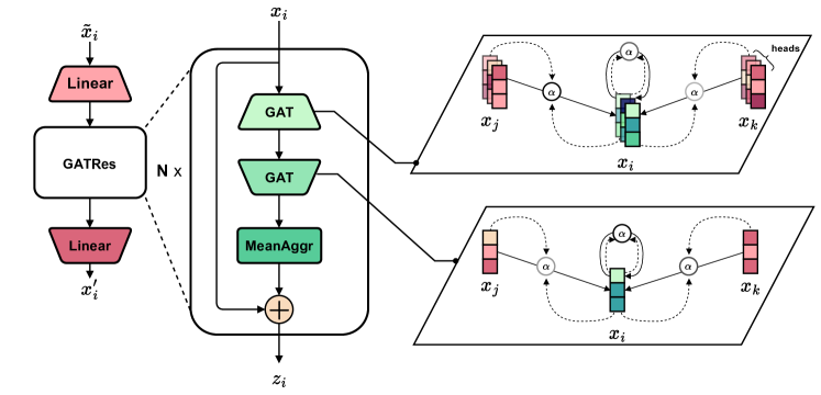
Figure 3: GATRes architecture. The left image indicates the overall architecture consists of two linear layers interleaving with GATRes blocks. The middle figure illustrates the abstract view in each block. The right-side ones explain the message aggregation mechanism between neighbor nodes.

As in the middle image in Figure 3, we feed the intermediate input $x_{i}$ to two GAT layers sequentially. For a target node $i$, the inner $GAT:\mathbb{R}^{N\times d_{in}}\rightarrow\mathbb{R}^{N\times Hd_{out}}$ devises multi-head views and weighs them among its 1-hop neighbors. In other words, it additionally enriches the diversity of multi-head views using the message aggregation from surrounding nodes.

Then, the outer $GAT:\mathbb{R}^{N\times Hd_{out}}\rightarrow\mathbb{R}^{N\times d_{out}}$ creates a bottleneck in the feature dimension and, again, reweights the target representation considering the ones of its neighbors. Note that the second GAT has exactly one head to transform all previous heads into a consistent view. We call this process a squeezing technique. Since most initial features are noise or zeros, squeezing can reduce the sparsity duplication in feature space caused by head concatenation and, therefore, benefits second attention among nodal pairs. Moreover, we consider the distribution of pressure values in the neighborhood, so we empirically apply a mean aggregator to the current representations (Xu et al.,, 2019). Afterward, we use a non-parametric residual connection with the intermediate input $x_{i}$ that allows depth extension and diminishes the overfitting problem (He et al.,, 2016).

As in Figure 3, the overall structure is a stack of numerous GATRes blocks. As each block considers 1-hop neighborhoods, stacking multi-blocks allows message propagation to faraway neighbors in the graph. Before message propagation layers, we employ a shared-weight linear transformation to project the masked input nodal features to higher-dimensional space. The details of masked inputs will be explained in the following subsection. We refer to the first linear layer as the steaming layer, which is well-known in computer vision tasks (Dosovitskiy et al.,, 2021; Tan and Le,, 2019). After message propagation, the final linear layer acts as a decoder to project higher-dimensional representations back to the original dimension (i.e., $d_{node}=1$). The end-to-end model will then output an immediate snapshot in which all pressure values at any junctions are recovered.

4.4 Model training

This section introduces our solution to leverage GATRes to solve the pressure estimation task. We first describe the general training scheme applied to any GNN model. Then, we provide an approach to test the trained model on time-relevant data. We also interpret why the proposed solution satisfies the criteria found in Section 3.

4.4.1 Training details

Pressure estimation is a semi-supervised node-level task. Concretely, it aims to predict missing node features in the entire graph, given limited known nodal information and graph-related properties. Due to the lack of historical data and sensor scarcity, we leverage nodal features $\mathcal{X}$ created in our data generation to form the training set.

To begin with, we sample a binary mask vector $m=\{m_{1},m_{2},...,m_{N}\}$ where each $m_{i}\in\{0,1\}$. We then construct a feature subset of the masked node $\tilde{\mathcal{X}}\subset\mathcal{X}$ in which its element $\tilde{x}_{i}$ is denoted as:

$$\tilde{x}_{i}=\begin{cases}0&m_{i}=1\\ x_{i}&m_{i}=0\end{cases}$$ (5)

There exist various masking strategies, such as learnable [MASK] tokens, feature permutation, arbitrary vector substitution, and mixup nodal features, which could be helpful for future work. In this work, we opt for a simple masking approach: replacing the node features with zeros in the masked positions to create the masked $\tilde{\mathcal{X}}$ (Equation 5). We then formalize the pressure estimation as follows:

$$\mathcal{X}^{\prime}=f_{GNN}(\tilde{\mathcal{X}},\mathcal{A},\mathcal{E};\Theta)$$ (6)

where $f_{GNN}:\mathbb{R}^{N\times d_{node}}\times\mathbb{R}^{N\times N}\times\mathbb{R}^{M\times d_{edge}}\mapsto\mathbb{R}^{N\times d_{node}}$ is a generic GNN function that takes partial-observable feature matrix $\tilde{\mathcal{X}}$, the topology $\mathcal{A}$, and edge attributes $\mathcal{E}$ as inputs and yields reconstructed features $\mathcal{X}^{\prime}$ characterized by model weights $\Theta$. The key idea is to find the optimal weights that satisfy the minimum error between predicted and ground truth nodal features. Mathematically, the objective is formalized as follows:

$$\Theta^{*}=\operatorname*{argmin}_{\Theta}\mathcal{L}(\mathcal{X}^{\prime},\mathcal{X})$$ (7)

Empirically, we use the mean square error (MSE) as a default loss function $\mathcal{L}$ for GATRes because it yields the best result in our tests. In addition, inspired by BERT (Devlin et al.,, 2018), the loss is computed on masked positions. After computation, model weights $\Theta$ are updated by the partial derivatives w.r.t the computed loss. For detail, we refer to gradient descent optimization techniques (Ruder,, 2016; Kingma and Ba,, 2014) . The training progress is then iterated with different masked features $\tilde{\mathcal{X}}$ derived from the original features $\mathcal{X}$ until the model convergence.

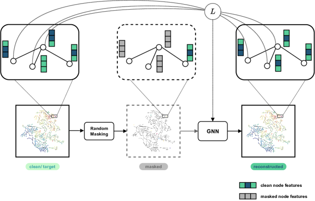
Figure 4: Graph Neural Network training scheme. Given clean snapshots, we mask out a significant number (95%) of node features. The remaining data is then sent into a GNN playing as an autoencoder to rebuild missing values with regard to graph properties (such as topology and edge attributes). GNN weights are updated using the loss derived by the predicted and ground truth values at masked places.

4.4.2 Testing details

In testing, the test graphs can be represented as $\mathcal{G}_{test}=\{\tilde{\mathcal{X}}_{test},\mathcal{A}_{test},\mathcal{E}_{test}\}$. By default, topology and edge attributes are retained as in training while $\tilde{\mathcal{X}}_{test}$ is varied and its data distribution is undetermined. For the generalization problem, $\mathcal{G}_{test}$ can differ from the training graphs in any property. In other words, the model should be able to estimate pressure on an unseen topology and an unknown data distribution.

With the time involved, the test graph at a particular time $t$ is denoted as $\mathcal{G}^{t}_{test}$. As the designed model takes only one snapshot as input, we feed temporal $\mathcal{G}^{t}_{test}$ into GATRes sequentially and individually. As a result, the reconstructed outcome does not affect the consecutive reconstructions during inference phase. In other words, this simple strategy isolates the model decision from the tendency to time-related data rarely found in training.

Developing data generation concerning time data and a temporal GNN is also possible, but it exponentially raises the cost of complexity and computation. Thus, we encourage further work to explore temporal models, timed data generation, and the trade-off between efficiency and performance in the future. In contrast, snapshot-based generators and GNNs ensure efficiency that satisfies practical needs (e.g. inference time).

4.4.3 Criteria satisfaction

Figure 4 illustrates the training scheme leveraging the synthetic dataset to solve the pressure estimation task on practical data. We remark that it satisfies the predefined criteria: $\bm{(\mathbb{C}1)}$ by GATRes being a spatial-based GNN approach that has topology awareness in its decision, $\bm{(\mathbb{C}2)}$ by random masking that dynamically changes sensor positions and myriad contextual snapshots from our data generation tool, and $\bm{(\mathbb{C}3)}$ by effectively evaluating the model on unseen time-relevant data with respect to uncertainty conditions.

5 Experiment settings

5.1 Datasets

The main use case in this study was performed using a private large-scale WDN in The Netherlands in the area of Oosterbeek. The network comprises 5855 junctions and 6188 pipes. Figure 5(a) shows the topology and the pressures at the nodes from some random snapshot of Oosterbeek WDN.

We also used four publicly available WDNs benchmarks, namely Anytown (Walski et al.,, 1987), C-Town (Ostfeld et al.,, 2012), L-Town (Vrachimis et al.,, 2022), and Richmond (Van Zyl,, 2001) to provide a baseline for evaluation and reproducibility of our work . Finally, in the experiments related to model generalization, we used two additional public datasets, Ky13 (Hernadez et al.,, 2016) and an anonymized WDN called “Large” (Sitzenfrei et al.,, 2023). The WDNs used in this study vary is size and structure, ranging from small and medium size to large-scale networks like “Large” and Oosterbeek, as can be seen in Figure 5. Table 2 shows the main characteristics of each network.

Figure 5: Water Distribution Networks used in this study.

Table 2: Properties of WDNs used in this study.

WDNs:	Oosterbeek	Anytown	C-Town	L-Town	Richmond	Ky13	Large
$junctions$	5855	22	388	785	865	775	3557
$pipes$	6188	41	429	909	949	915	4021

5.2 Baseline models settings

Generally, two goals dictate the baseline selection. Section 3 mentions the first goal: to try out popular GNN architectures on a node-level regression problem. The aim is to achieve acceptable errors when the models are tested on data points that are from an unknown “nature” distribution. The second goal is to explore existing frameworks, from synthesized data querying and model training to evaluation phases. We aim to establish a reliable benchmarking framework for pressure estimation tasks or problems related to water distribution networks. In other words, the model that performs better in our tests should be more useful in practical applications.

For this purpose, we compare our GATRes architecture to popular GNNs, including GCNii (Chen et al., 2020b, ) and GAT (Veličković et al.,, 2018). In addition to this, GraphConWat (GCW) (Hajgató et al.,, 2021) and mGCN (Ashraf et al.,, 2023), which are dominant approaches in solving pressure estimation using GNN with sparse information, are also considered in our comparison. Table 3 summarizes the model settings. It is worth noting that we uniquely employ the best settings in each model across all considered WDNs to guarantee $\bm{(\mathbb{C}1)}$ satisfaction.

Table 3: Baseline settings.

	GCNii	GAT	GCW	0.11GCW
tuned
(ours)	mGCN	0.11GATRes
small
(ours)	0.11GATRes
large
(ours)
#blocks	64	10	4	4	45	15	25
#hidden.channels	32	{32,64}	{120,60,30}	32	{98,196}	{32,64}	{128,256}
Coefficient K	-	-	{240,120,20,1}	{24,12,10,1}	-	-	-
Loss	MSE	MSE	MSE	MSE	MAE	MSE	MSE
Learning Rate	3e-4	3e-4	3e-4	3e-4	1e-5	5e-4	5e-4
Weight Decay	1e-6	1e-6	1e-6	1e-6	0	1e-6	1e-6
Edge Attribute	binary	binary	binary	binary	pipe.len, pipe.diaa	binary	binary
Norm Type	znorm	znorm	minmax	znorm	minmax	znorm	znorm
a Pipe lengths and pipe diameters. They are static parameters gathered from the corresponding Water Distribution Network.

GATRes-small with hyperparameters is the optimal version after the optimization process, which will be carefully explained in the latter section. To study the impact of the model size, we also introduce GATRes-large scaling close to mGCN in terms of the number of parameters.

GAT remained at a shallow depth to prevent the oversmoothing problem (Chen et al., 2020a, ). Precisely, neighbor features encoded by a too-deep GNN converged to indistinguishable embeddings that harm the model performance. Empirically, we balance the trade-off between performance and efficiency for each model to select the appropriate hyperparameters.

In GraphConvWat models, we detached binary masks from the input features as these masks did not improve the model performance, which aligns with the findings in (Ashraf et al.,, 2023). Furthermore, GraphConvWat tuned is a lightweight version in which the degrees of the Chebyshev polynomial $K_{i}$ are set to smaller values to reduce complexity and work surprisingly well in our experiments.

Training mGCN slightly diverged from its original work in sensor positions. Concretely, (Ashraf et al.,, 2023) trained mGCN using fixed sensors with extensive historical data. However, as we explained in Section 4.4, this data was inaccessible throughout training. Therefore, we fed different random masks into the model in each epoch. Considering a synthetic dataset, the model had an opportunity to capture meaningful patterns in various sensor positions.

5.3 Evaluation metrics

The most common evaluation metrics used for assessing the performance of regression models are Root Mean Square Error (RMSE), Mean Absolute Error (MAE) and Mean Absolute Percentage Error (MAPE) (Zhao et al.,, 2019; Derrow-Pinion et al., 2021b, ; Jiang and Luo,, 2022). We consider important to use evaluation metrics which are common not only in the Machine Learning domain, but also in hydrologic sciences. Following the insights from (Legates and McCabe Jr.,, 1999), the models should be evaluated using both, relative and absolute error metrics. Thus, our model is evaluated using MAE and MAPE. Additionally, we included the Nash and Sutcliffe Coefficient of Efficiency (NSE), widely used to evaluate the performance of hydrologic models (Legates and McCabe Jr.,, 1999). Finally, we used an accuracy metric defined as the ratio of positive predictions over the total number of predicted values. The positive predictions are those that deviates at most a certain threshold $(\delta_{\text{thresh}})$ from the true value. Thus, the evaluation metrics used in this work are defined as follows:

$$\text{MAE}=\frac{1}{N}\sum_{i=1}^{N}|y_{i}-\hat{y}_{i}|$$ (8)

$$\text{MAPE}=\frac{1}{N}\sum_{i=1}^{N}\frac{|y_{i}-\hat{y}_{i}|}{y_{i}}$$ (9)

$$\text{NSE}=1-\frac{\sum_{i=1}^{N}({y_{i}-\hat{y}_{i}})^{2}}{\sum_{i=1}^{N}({y_{i}-\overline{y}})^{2}}$$ (10)

$$acc(@\delta_{\text{thresh}})=\frac{1}{N}\sum_{i=1}^{N}{positive_{i}}~{};~{}~{}~{}positive=\begin{cases}1,&\text{if}~{}|y_{i}-\hat{y}_{i}|\leq\delta_{\text{thresh}}*y_{i}\\ 0,&\text{otherwise}\end{cases}$$ (11)

where $\bm{y}$ denotes the true values, $\bm{\hat{y}}$ denotes the predicted values, $\bm{\overline{y}}$ is the mean of the true values, and $\bm{N}$ is the number of values to predict.

6 Experiments

6.1 Baseline comparison on Oosterbeek WDN

In this experiment, we investigated the proposed model performance against GNN variants on a large-scale WDN benchmark called Oosterbeek. Specifically, given the topology and hydraulic-related parameters, our dataset generation provided 10,000 synthetic snapshots divided into 6000, 2000, and 2000 for training, validation, and testing sets, respectively. However, as we discussed in Section 2.2, these synthetic sets might not reflect real-world scenarios. Therefore, we merely used them to keep track of model learning during the training process.

Alternatively, we performed the comparison on the Oosterbeek dataset recorded every five minutes for 24 hours. We relied on mathematical simulation to produce reproducible results that resembled real-world conditions. The topology and predefined parameters set by hydraulic experts under a calibration process made them valid for our analysis. As a result, we considered the simulated outcomes of time-relevant data as ground truths. However, it was essential to acknowledge that specific hydraulic parameters, such as customer demands and pipe roughness, remained undetermined due to the dimensional explosion in parameter space, leading to noticeable errors in practical scenarios (Zhou et al.,, 2023). To replicate this uncertainty, we utilized a distortion approach on junction demands during the testing phase inspired by (Zhou et al.,, 2023; Mücke et al.,, 2023). We then listed two testing strategies in detail as follows.

1. Clean test. We assumed there was no uncertainty in this test so that baseline models could observe clean, calibrated simulation pressures. Noticeably, because they all considered snapshots as individual samples, we can sample random masks indicating the visible virtual sensors per snapshot in every run. Running 100 times with diverse measurement locations would show the model capability in perfect condition.

2. Noisy test. Following (Zhou et al.,, 2023), we injected Gaussian noise into junction demands before the simulation was processed and then paired each outcome snapshot with a random mask for a test case. We set a tougher noise that went beyond the original tests. The new noisy test involved the mean and standard deviation of 10% and 100% of the initial demands, respectively. We ran 100 test cases and reported statistical findings.

Table 4: Model comparison in the clean test performed on 24-hour Oosterbeek WDN at 95% masking rate.

Model	0.1#Milion Params($\downarrow$)	MAE($\downarrow$)	1.3cmMAPE($\downarrow$)	NSE($\uparrow$)	Acc(@0.1)($\uparrow$)
GCNii (Chen et al., 2020b, )	0.65	6.357$\pm$0.0197	0.2147$\pm$0.0008	-0.0137$\pm$0.0061	38.48$\pm$0.1351
GAT (Veličković et al.,, 2018)	0.35	3.726$\pm$0.0120	0.1287$\pm$0.0008	0.3276$\pm$0.0037	73.52$\pm$0.0900
GraphConvWat (Hajgató et al.,, 2021)	0.92	3.067$\pm$0.0077	0.1160$\pm$0.0004	0.6938$\pm$0.0020	69.92$\pm$0.1205
GraphConvWat-tuned	0.23	2.293$\pm$0.0087	0.0821$\pm$0.0005	0.7518$\pm$0.0024	83.03$\pm$0.1025
mGCN (Ashraf et al.,, 2023)	2.48	2.111$\pm$0.0085	0.0806$\pm$0.0003	0.7100$\pm$0.0030	84.05$\pm$0.0693
GATRes-small (ours)	0.66	1.937$\pm$0.0074	0.0703$\pm$0.0005	0.7773$\pm$0.0025	87.48$\pm$0.0761
GATRes-large (ours)	1.67	2.020$\pm$0.0132	0.0711$\pm$0.0003	0.7864$\pm$0.0031	84.33$\pm$0.1347

Table 5: Model comparison in the noisy test performed on 24-hour Oosterbeek WDN at 95% masking rate.

Model	0.1#Milion Params($\downarrow$)	MAE($\downarrow$)	1.3cmMAPE($\downarrow$)	NSE($\uparrow$)	Acc(@0.1)($\uparrow$)
GCNii (Chen et al., 2020b, )	0.65	6.696$\pm$0.0838	0.2484$\pm$0.0552	-0.1064$\pm$0.0266	36.02$\pm$0.4684
GAT (Veličković et al.,, 2018)	0.35	4.397$\pm$0.3052	0.2112$\pm$0.0767	0.1490$\pm$0.1153	66.98$\pm$1.6290
GraphConvWat (Hajgató et al.,, 2021)	0.92	3.611$\pm$0.1234	0.1551$\pm$0.0376	0.5877$\pm$0.0370	62.99$\pm$1.1600
GraphConvWat-tuned	0.23	2.347$\pm$0.0252	0.0963$\pm$0.0363	0.749$\pm$0.0086	81.09$\pm$0.3877
mGCN (Ashraf et al.,, 2023)	2.48	2.188$\pm$0.0558	0.0948$\pm$0.0155	0.6993$\pm$0.0213	82.83$\pm$0.4199
GATRes-small (ours)	0.66	1.964$\pm$0.0301	0.0802$\pm$0.0458	0.778$\pm$0.0113	86.56$\pm$0.2826
GATRes-large (ours)	1.67	2.115$\pm$0.0503	0.0799$\pm$0.0207	0.7417$\pm$0.0140	83.43$\pm$0.5044

Regarding the experimental setting, we trained all models in 500 epochs with a batch size of 8 for a fair comparison among the baseline models. Early Stopping was applied to suppress training if the validation error had no improvements in 100 steps. We used Adam optimizer (Kingma and Ba,, 2014) and set the default masking rate at 95%, leaving only 5% of nodes unmasked.

For evaluation, we tested the baseline models on the 24-hour Oosterbeek, repeating the process a hundred times. The mean and standard deviation of the results are presented in Table 4. Unless otherwise specified, the default is a clean test in our experiments. The results of the noisy test are given in Table 5.

Table 4 shows that GATRes-small achieved accurate junction pressure reconstruction with an average relative error of 7% and an absolute error of 1.93 water column meters, even with a sparse masking ratio of 95%. Notably, the testing data were time-sensitive and originated from an unfamiliar distribution our models were not exposed to during training. The good results on snapshot-based models suggest that in case temporal data is not available, snapshot-based models seem to be good alternatives.

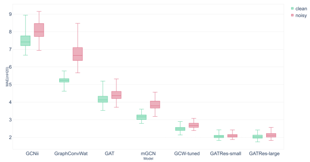
Figure 6: Baseline Mean Absolute Errors measured for a single snapshot under both clean and noisy conditions.

Our next focus was on analyzing the baseline robustness. Precisely, we assessed each baseline on clean and noisy tests using an individual snapshot with a hundred randomly initialized masks. Our primary objective was to measure the model’s robustness in these contrasting scenarios. A superior model should exhibit minimal error discrepancy between them. As illustrated in Figure 6, both versions of GATRes consistently maintained similar error levels even under conditions of high uncertainty. In contrast, other models exhibited a noticeable gap in their results when transitioning from clean to noisy environments.

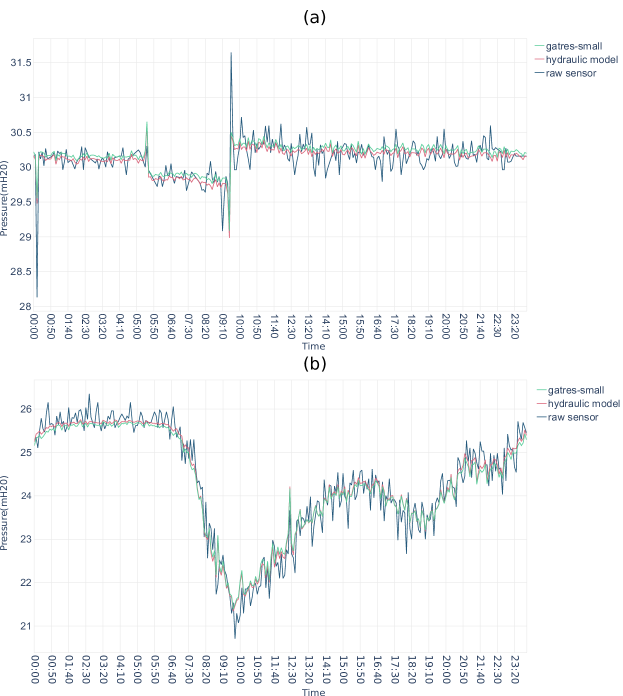
Figure 7: Pressure values estimated on other actual sensors

Finally, we conducted a detailed analysis of our top-performing model, GATRes-small, based on the evaluations conducted earlier. In this analysis, we intentionally covered sensor locations to observe model inference on those nodes. Figure 7 illustrates time series data from the predictions of GATRes-small, a well-calibrated simulation, and actual meter readings. As expected, GATRes closely mirrors the behavior of the hydraulic simulation, demonstrating sufficient capability of a desired surrogate model. Although a slight difference exists between them, both time series were bounded in the range of actual measurements.

6.2 Generalization

This set of experiments are the first attempts aimed to achieve generalization capabilities of our model. We want to evaluate whether training a model on different topologies simultaneously can equip the model with generalization capabilities. For this, we chose three different WDNs, which topologies vary in structure and size.

First, we trained GATRes-small on L-Town, Ky13 and “Large” WDNs simultaneously. This model is named as Multi-Graph model. We wanted to evaluate the performance of this model on a fully unseen topology. Hence, we executed Zero-Shot inference (predict on a WDN topology not seen during training) using the Multi-Graph model on our main use case Oosterbeek WDN. This model was trained with the ReduceLROnPlateau learning rate scheduler from Pytorch library. The scheduler reduces the learned rate if the model does not improve for a certain number of epochs. This model was trained with a batch size of 16 for 500 epochs. The initial learning rate was set to 5$e$-3 and it is reduced by a factor of $0.1$ if the validation loss does not improve for $30$ consecutive epochs.

A second experiment is transfer learning, a technique motivated by the fact that humans use previously learned knowledge to solve new tasks faster or better (Pan and Yang,, 2009). Hence, the learned weights by a model trained on some particular network(s) can be transferred to train and improve the prediction capabilities of a model on a new, previously unseen WDN. We applied transfer learning and fine-tuning, which involves using the weights of a pre-trained model on a source dataset to initialize the weights of the new model that will be trained on the target dataset.

In our work, the pre-trained model is the Multi-Graph model, trained on L-Town, Ky13 and “Large”, and the Fine-Tuned model has as the target the Oosterbeek WDN. Usually, during fine-tuning, the top layers of the pre-trained model are frozen and reused as feature extractors for the target data. We empirically found that unfreezing the entire model and retraining all layers produces better results. Thus, we initialized the weights of the target model with those of the pre-trained one. Then, we reduced the learning rate for training the target model to avoid completely changing the pre-trained weights during fine-tuning. The learning rate was reduced from 5$e$-3 in the source model to 1$e$-4 during fine-tuning. The target model was trained with a batch size of 8 for 200 epochs. The results of these experiments are shown in Table 6. They reflect those of (Yosinski et al.,, 2014) who also found that combining transfer learning with fine-tuning shows better performance than a model trained directly on a target dataset.

Table 6: Generalization evaluation on 24-hour Oosterbeek WDN

	MAE ($\downarrow$)	MAPE ($\downarrow$)	NSE ($\uparrow$)
GATRes-small	1.9370 $\pm$0.0074	0.0703 $\pm$0.0005	0.7773 $\pm$0.0025
Multi-Graph (Zero-Shot)	3.0597 $\pm$0.0074	0.0998 $\pm$0.0005	0.5700 $\pm$0.0045
Fine-tuned	1.9097 $\pm$0.0076	0.0695 $\pm$0.0005	0.7980 $\pm$0.0030

6.3 The effect of masking ratios

To explore the model capability, we investigated the GATRes-small on myriad masking rates. Identical to the previous experiment, the model was trained on the synthetic dataset generated from our algorithm and performed a clean test on the 24-hour data. Both were devised from the Oosterbeek WDN. In addition, each GATRes-small corresponding to a specific mask rate was trained within 200 epochs with the default settings. For convenience, we replaced the model name with fixed masking rates in this experiment.

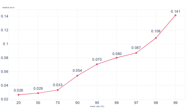
Figure 8: Relative errors (MAPE) for nodal pressure on different masking ratios(lower is better).

Figure 8 shows the influence of the masking ratio on the proposed model. Each ratio indicates a specific probability of missing nodal features (i.e., the pressure signals in a snapshot graph). Due to the sensor density being exceptionally sparse in real-world scenarios, the typical benchmark of 95%, commonly found in previous studies, is deficient in reflecting this practical issue. Therefore, we report errors occurring in all cases with lower and more extreme ratios that exceed the standard. Additional metrics are found in Table 7.

Table 7: Detailed performance of GATRes-small on different masking ratios.

Mask ratio(%)	MAE($\downarrow$)	MAPE($\downarrow$)	NSE($\uparrow$)	Acc(@0.1)($\uparrow$)
20	0.610	0.0265	0.9599	0.9760
50	0.798	0.0286	0.9372	0.9654
70	0.900	0.0331	0.9301	0.9586
90	1.457	0.0544	0.8603	0.9167
95	1.939	0.0703	0.7770	0.8746
96	2.213	0.0800	0.7185	0.8467
97	2.415	0.0867	0.7059	0.8148
98	3.075	0.1091	0.5648	0.7465
99	4.087	0.1414	0.3424	0.6396

6.4 Baseline comparison on benchmark WDNs

In this set of experiments we compared the performance of GATRes-small against two state-of-the-art baseline models, GraphConvWat (Hajgató et al.,, 2021) and mGCN (Ashraf et al.,, 2023). We evaluated the three models on four benchmark WDNs: Anytown, C-Town, Richmond, and L-Town, described in Section 5.1. The data used in these experiments were created following the method proposed by (Hajgató et al.,, 2020) to facilitate comparability under the original conditions defined by previous works. We created 1,000 snapshots for Anytown, 10,000 snapshots for C-Town and L-Town, and 20,000 snapshots for Richmond. Then, the datasets were split into training, validation and test sets in a 6:2:2 ratio.

We used the same experimental settings as proposed in the baseline approaches to guarantee a fair comparison. Thus, in all experiments the models are trained for 2,000 epochs with early stopping, using the Adam gradient-based optimization algorithm (Kingma and Ba,, 2014). The GraphConvWat model training was stopped if the validation loss did not improve for 50 consecutive epochs. In the case of mGCN, the training was stopped if no improvement is seen after 250 epochs. Likewise mGCN, our model training is stopped after 250 epochs if no improvement is observed. In all cases, it is considered an improvement when the validation loss decreases at least by 1e-6.

The evaluation of the models’ performance on each WDN, with the exception of Anytown, was using data that included realistic demand patterns per node. In the case of C-Town and Richmond, the WDN snapshots for evaluation were created using a 24-hour demand pattern time series sampled at 5 minutes interval. L-Town evaluation snapshots were created using a 1-week demand pattern time series sampled at 5 minutes interval. Table 8 shows the results of the performance comparison of ten runs per WDN, and then the mean and standard deviation are reported. As can be seen from the table, our model GATRes-small achieves the lowest MAE in all WDNs and the lowest MAPE in all networks but Richmond. Likewise, GATRes-small achieves the higher NSE in all WDNs but Richmond.

Table 8: Models performance comparison on 24-hour demand pattern time series data.

WDN	Metrics	Models
		GraphConvWat	mGCN	GATRes-small (ours)
C-Town	MAE ($\downarrow$)	14.8860 $\pm$0.1418	19.9138 $\pm$0.0948	09.4860 $\pm$0.1822
	MAPE ($\downarrow$)	0.1028 $\pm$0.0009	0.1318 $\pm$0.0005	0.0690 $\pm$0.0010
	NSE ($\uparrow$)	0.7870 $\pm$0.0046	0.6310 $\pm$0.0030	0.8480 $\pm$0.0075
Richmond	MAE ($\downarrow$)	4.3501 $\pm$0.0170	2.9690 $\pm$0.0283	2.8114 $\pm$0.0899
	MAPE ($\downarrow$)	0.0196 $\pm$0.0001	0.0128 $\pm$0.0002	0.0133 $\pm$0.0005
	NSE ($\uparrow$)	0.9500 $\pm$0.0000	0.9630 $\pm$0.0046	0.9390 $\pm$0.0030
L-Town	MAE ($\downarrow$)	3.4505 $\pm$0.0129	1.5928 $\pm$0.0050	0.9501 $\pm$0.0086
	MAPE ($\downarrow$)	0.0611 $\pm$0.0002	0.0305 $\pm$0.0001	0.0157 $\pm$0.0002
	NSE ($\uparrow$)	0.5040 $\pm$0.0049	0.8000 $\pm$0.0000	0.9000 $\pm$0.0000

One limitation of previous approaches is the evaluation of model performance on unrealistic data, i.e., an exact copy of the training data distribution (Section 2.2). In previous approaches, the snapshots representing random WDN states used for training, validation and test are created by the same algorithm. Consequently, the distribution of the data used for testing is a fidelity copy of the data used for training. However, in practice, the distribution of the real data differs from the data used for training the reconstruction models, as explained in Section 2.2. Therefore, it is important that the models adapt to circumvent such uncertainties. Previous approaches achieve impressive performance when tested on replicas of the training data (see Table 9), but the performance drop is evident when they are evaluated on a realistic scenario (see Table 8).

Table 9: Models performance comparison on synthetic sampling-based snapshots following (Hajgató et al.,, 2020) approach.

WDN	Metrics	Models
		GraphConvWat	mGCN	GATRes-small (ours)
Anytown	MAE ($\downarrow$)	5.1044 $\pm$0.0714	3.9460 $\pm$0.0642	3.9245 $\pm$0.1056
	MAPE ($\downarrow$)	0.0654 $\pm$0.0012	0.0497 $\pm$0.0009	0.0491 $\pm$0.0012
	NSE ($\uparrow$)	0.7440 $\pm$0.0049	0.8020 $\pm$0.0075	0.7980 $\pm$0.0189
C-Town	MAE ($\downarrow$)	4.1619 $\pm$0.0170	1.6963 $\pm$0.0133	1.8928 $\pm$0.0149
	MAPE ($\downarrow$)	0.0354 $\pm$0.0001	0.0148 $\pm$0.0001	0.0169 $\pm$0.0001
	NSE ($\uparrow$)	0.9640 $\pm$0.0049	0.9900 $\pm$0.0000	0.9900 $\pm$0.0000
Richmond	MAE ($\downarrow$)	2.3999 $\pm$0.0069	0.6363 $\pm$0.0061	1.5979 $\pm$0.0106
	MAPE ($\downarrow$)	0.0110 $\pm$0.0000	0.0029 $\pm$0.0000	0.0080 $\pm$0.0001
	NSE ($\uparrow$)	0.9805 $\pm$0.0003	0.9900 $\pm$0.0000	0.9750 $\pm$0.0009
L-Town	MAE ($\downarrow$)	1.2970 $\pm$0.0036	0.2441 $\pm$0.0014	0.4930 $\pm$0.0028
	MAPE ($\downarrow$)	0.0159 $\pm$0.0000	0.0030 $\pm$0.0000	0.0061 $\pm$0.0000
	NSE ($\uparrow$)	0.9700 $\pm$0.0000	1.0000 $\pm$0.0000	1.0000 $\pm$0.0000

The density distributions of training and test sets in C-Town, Richmond and L-Town WDNs are shown in Figure 9. It is clear that the distributions of the training and testing data created by the same algorithm (mathematical simulation) are identical, while the distribution of the test data with a demand pattern greatly differs from the one used during training. This shows the ability of GATRes to adapt to the changes that occur in real life scenarios. It also shows that other models achieve better results only when evaluated on fidelity copies of the training data, caused by overfitting due to the large model complexity of the previous approaches. The density distribution plot in Figure 9(b) explains the good performance of mGCN on Richmond WDN in terms of MAPE and NSE (Table 8), the time-based demand pattern test dataset has a similar distribution than the one used for training.

Figure 9: Comparison of density distributions of synthetic and time-based datasets in C-Town, Richmond and L-Town WDNs.

6.5 Ablation study

The ablation study presented in this section evaluates the importance of the different components of GATRes model architecture, and the effect of their removal or alteration on performance. In every run, a specific component is removed or altered, and GATRes is restored to its original version before a new change is made. The different variants used in the ablation study are the following:

• Without Residual Connections (woResCon). The residual connections used within each GATRes Block are removed.

• Without Mean Aggregation (woMeanAggr). The Mean Aggregation applied after the second convolution within each GATRes Block is removed and the residual connection is added to the output of the second convolution.

• Without Residual Connection and Without Mean Aggregation (woResCon-woAggr). Both, the residual connection and the mean aggregation are removed from the GATRes Block.

• Mean Aggregation Outside the Block (MeanAggrOut). Instead of applying a mean aggregation within each block, it is applied only once in the forward pass, after the output of the last GATRes Block and before the final Linear layer.

These experiments were performed by training GATRes-small on the C-Town WDN. As can be seen in Table 10, removing the Residual Connections produced the highest negative impact on model performance for all metrics.

Table 10: Ablation study of GATRes evaluated on C-Town 24-hour time series data.

Variants	MAE ($\downarrow$)	MAPE ($\downarrow$)	NSE ($\uparrow$)
GATRes-small	09.4860 $\pm$0.1822	0.0690 $\pm$0.001	0.8480 $\pm$0.0075
woMeanAggr	09.7479 $\pm$0.1444	0.0686 $\pm$0.0009	0.8473 $\pm$0.0046
woResCon-woAggr	10.0934 $\pm$0.1644	0.0735 $\pm$0.0010	0.8150 $\pm$0.0062
MeanAggrOut	10.3735 $\pm$0.1251	0.0735 $\pm$0.0006	0.8333 $\pm$0.0058
woResCon	11.5362 $\pm$0.1697	0.0815 $\pm$0.0008	0.7694 $\pm$0.0089

7 Discussion

In this section, we generally discuss our findings and technical changes that affect our model in estimating pressures on Water Distribution Networks. We first review changes that made GATRes versions outperform other baselines and their limitations. Then, we discuss the role of synthetic data and the relationship between hydraulic simulation and surrogate models. Finally, we address the question of generalizability in the context of our research.

7.1 General findings and limitation

GATRes qualified all criteria for model assessment as in Section 4.4.3 and achieved pressure reconstruction with an average relative error of 7% and an absolute error of 1.93 water column meters on a 95% masking rate (see Table 4). We attribute its success primarily to the fundamental blocks and training strategy. These blocks update the weights of connections using nodal features and, therefore, relax the original topology in a given Water Distribution Network. This relaxation provides robustness and generalizability to GATRes in uncertain conditions and across diverse network topologies, which may vary in size, headloss formula, and component configurations. Furthermore, GATRes utilizes a random sensor replacement strategy, eliminating the need for time-consuming retraining when a new sensor is introduced in the future. For these reasons, both blocks within the architecture and training strategy sharpen a GATRes as a highly reusable and sustainable solution for predicting pressures in numerous Water Distribution Networks.

However, it is essential to acknowledge the limitations when GATRes comes to scale. The limit becomes apparent when comparing the larger and smaller versions of GATRes in Tables 4 and 5. The larger GATRes eventually reaches a saturation point of performance and is surpassed by its smaller counterpart. The same finding is available in both GATConvWat variants. They likely originate from inherent issues in graph neural networks, such as over-smoothing and over-squashing, where nodes tend to propagate redundant information excessively (Di Giovanni et al.,, 2023). While GATRes employs residual connections that partially mitigate the over-smoothing and mainly contribute to the model performance, as shown in Section 6.5, they are unable to eliminate this phenomenon completely (Kipf and Welling,, 2017). To address these issues in the future, potential solutions may include exploring graph rewiring strategies and subgraph sampling techniques.

7.2 Benefit of synthetic data

Throughout our experiments, the integration of data generated by our innovative tool has proven to be a game-changer when it comes to training deep models. Those results not only achieve remarkable accuracy but also indicate the helpfulness of synthetic data, especially when sensor records or simulation parameters are restricted. Indeed, these common issues have been found in many public benchmarks, such as five reviewed water networks in Section 5.1, due to the missing historical patterns and privacy issues. They have made reproducibility a persistent challenge in water network research.

As a solution, our data generation tool extends the limits in approaching these public networks without confidential matters. For practical purposes, the synthesized training set could involve as many cases as possible, reducing the risk of long-term incidents that may not have occurred in historical records. Thus, it boosts model robustness when dealing with unforeseen scenarios.

7.3 Relationship between hydraulic simulations and GATRes

Yet, an intriguing question arises: Can we replace traditional mathematical simulations with surrogate models like GATRes? Conventional simulation bridges the interaction between hydraulic experts and the Water Distribution Network in water management. Such an interaction should be preserved in the design or analysis phase. In the deployment, especially for Digital Twin or water systems on big data, pressure estimate models often deal with heavy computation and require a low response time (Pesantez et al.,, 2022). In this case, GATRes and GNN variants can be alternative approaches due to their competitive results and impressive throughput (see Table LABEL:tab:throughput). However, these deep models may involve the risk of over-relaxation of energy conservation laws and other constraints within the actual networks. The risk is often minimal in pure physics-based simulations.

Accordingly, these simulations still play a critical role in data synthesis as they define a valid boundary for newly created models thanks to their generated training samples and testing environments. When fast computation is required, GATRes is a good alternative to estimate the pressure of a large WDN given unlimited sensor streams. In the future, it is potential to focus on physics-inspired models that can regularize GATRes to preserve fundamental physical laws and yield more confident results.

7.4 Generalization

GATRes is able to generalize to previously unseen WDNs by design given the ability of spatial methods (e.g. GAT) to generalize across graphs (Bronstein et al.,, 2017). On the contrary, previous works that rely on spectral approaches suffer from the generalization problem because their convolutions (e.g. ChebNet) depend on the eigen-functions of the Laplacian matrix of a particular graph (Zhang et al.,, 2019).

GATRes trained on multiple WDNs simultaneously produced a MAE of 3.06mH₂O and a MAPE of 9.98%, on average, at zero-shot inference on 24-hour Oosterbeek WDN. These results are impressive given that pressure estimation was performed on a completely different, previously unseen, WDN. Moreover, the fine-tuned model, on the target dataset Oosterbeek, produced a reduction in MAE of 1.51% with respect to the model trained directly and only on Oosterbeek.

The results of our first attempts towards generalization (see Table 6) show that our approach is worth further exploration. GNN models fail to generalize when the local structures of the graphs in the training data differ from the local structures in the test data (Yehudai et al.,, 2021). Then, a possible explanation of the generalization capabilities of GATRes is the training on several WDNs simultaneously. Using graphs that differ in size and structure, for training, allows GATRes to learn a richer set of local structures that may be present in the target WDN. Despite these promising results, several questions remain unanswered. For example, how to choose the right WDNs in order to enrich the training data in terms of local structures’ diversity? How to design a pre-trained task that can effectively capture the local-level patterns and extrapolate those to unseen larger graphs? How to train a GNN-based foundation model, in the Water Management Domain, that can be applied on different downstream tasks on any WDN topology? All these questions open paths for future research directions.

8 Conclusions

In this work we presented a hybrid, physics-based and data-driven, approach to address the problem of state estimation in WDNs. We leveraged mathematical simulation tools and GNNs to reconstruct the missing pressures at 95% of the junctions in the network, from only 5% of them seen during training. We also tested our approach on more extreme cases of sensor sparcity, reaching up to 99% masking rate. Our work proposes a number of research contributions. First, a new training data generation process that does not consider time-dependent patterns and includes control parameters for the simulation that were fully overlooked in previous works. This results in a more diverse training dataset and avoids uncertainty propagation due to model simplification errors. In addition, our random masking strategy during training provides robustness against sensors’ location changes due to new installations or maintenance. Moreover, the proposed evaluation method considers real time-dependent patterns and Gaussian noise injection, producing the out-of-distribution data intrinsic to real-world scenarios. Thus, enabling the resilience of the model to unexpected circumstances. Furthermore, a multi-graph pre-training strategy followed by fine-tuning allowed to improve the performance of the model with respect to the one trained and evaluated on a single topology.

Our model was evaluated on a large-scale network in The Netherlands, as well as on several WDNs benchmark datasets, showing a clear improvement over previous approaches. GATRes obtained an average MAE of 1.94mH₂O, which represents an 8.57% improvement with respect to other models. Similarly, it showed a reduction of MAE up to $\approx$52% on other WDN benchmarks, in the best cases, with respect to previous approaches. We attribute the high performance of GATRes to its building blocks and training strategy. These blocks relax the original topology leveraging nodal features to re-weight the connections by means of an attention mechanism. Despite its success, there are still some aspects that demand further exploration. On the one hand, while the residual connections mitigate the over-smoothing problem, inherent to GNNs, the phenomenon is not completely removed. Therefore, other techniques such as graph rewiring and subgraph sampling would be a fruitful area for further work. On the other hand, our multi-graph pre-training strategy is a promising direction towards model generalization and transferability in the WDNs domain. Nonetheless, further research needs to examine more closely the links between the topologies of the WDNs chosen for pre-training, the pre-training task, and their effect on the generalization capabilities of the model.

Data Availability Statement

In this section, we provide an overview of the publicly available benchmark water distribution networks and libraries that were employed in our study. Specifically, three networks, including Anytown (Walski et al.,, 1987), C-Town (Ostfeld et al.,, 2012), and Richmond (Van Zyl,, 2001), have been collected on Github (Hajgató et al.,, 2021). The L-town dataset is referenced in the paper by (Vrachimis et al.,, 2022), while the Ky13 benchmark (Hernadez et al.,, 2016) can be readily obtained via a free download on https://www.uky.edu/WDST/database.html. The “Large" network is referenced in the “Availability of Data and Materials" section in (Sitzenfrei et al.,, 2023). The Oosterbeek water network is not publicly available, as it is provided under confidentiality by the water provider Vitens.

In terms of libraries, we employed Matplotlib version 3.7.1 (Hunter,, 2007) (licensed under BSD) and Plotly version 5.15 (Inc.,, 2015), licensed under MIT, to craft our visual figures. The data generation tool was constructed using the Epynet wrapper, available on https://github.com/Vitens/epynet, and is licensed under Apache-2.0. We also leveraged the WNTR library (Klise et al.,, 2018), and Ray version 2.3.1 (Moritz et al.,, 2018) in our implementation.

Our datasets are organized in the zarr format, a file storage structure created using the Zarr-Python package version 2.14.2 (Miles et al.,, 2020), which is licensed under MIT. These datasets were employed in training both baseline models and GATRes variants using PyTorch (Paszke et al.,, 2019) and PyTorch Geometric (Fey and Lenssen,, 2019). We also tracked the training using tracking tools such as Wandb (Biewald,, 2020) and Aim (Arakelyan et al.,, 2020). The dataset generation tool and GATRes models are open-sourced at https://github.com/DiTEC-project/gnn-pressure-estimation.

Acknowledgments

This work is funded by the project DiTEC: Digital Twin for Evolutionary Changes in Water Networks (NWO 19454). We express our appreciation to Ton Blom and the Digital Twin group at Vitens, a Dutch drinking water company, for providing hydraulic knowledge and valuable data. Furthermore, we are grateful to Prof. A. Veldman for our insightful discussions. Also, we thank the Center for Information Technology of the University of Groningen for their support and for providing access to the Hábrók high performance computing cluster. We also thank M. Hadadian, F. Blaauw and Researchable for discussions about the experiments platform.

References

- Arakelyan et al., (2020) Arakelyan, G., Soghomonyan, G., and The Aim team (2020). Aim.
- Ashraf et al., (2023) Ashraf, I., Hermes, L., Artelt, A., and Hammer, B. (2023). Spatial graph convolution neural networks for water distribution systems. In International Symposium on Intelligent Data Analysis, pages 29–41. Springer.
- Barceló et al., (2020) Barceló, P., Kostylev, E. V., Monet, M., Pérez, J., Reutter, J., and Silva, J. P. (2020). The logical expressiveness of graph neural networks. In International Conference on Learning Representations.
- Bickel et al., (2007) Bickel, S., Brückner, M., and Scheffer, T. (2007). Discriminative learning for differing training and test distributions. In Proceedings of the 24th international conference on Machine learning, pages 81–88.
- Biewald, (2020) Biewald, L. (2020). Experiment tracking with weights and biases. Software available from wandb.com.
- Bonilla et al., (2022) Bonilla, C. A., Zanfei, A., Brentan, B., Montalvo, I., and Izquierdo, J. (2022). A digital twin of a water distribution system by using graph convolutional networks for pump speed-based state estimation. Water, 14(4):514.
- Bronstein et al., (2017) Bronstein, M. M., Bruna, J., LeCun, Y., Szlam, A., and Vandergheynst, P. (2017). Geometric deep learning: going beyond euclidean data. IEEE Signal Processing Magazine, 34(4):18–42.
- Campos et al., (2021) Campos, M. A. S., Carvalho, S. L., Melo, S. K., Gonçalves, G. B. F. R., dos Santos, J. R., Barros, R. L., Morgado, U. T. M. A., da Silva Lopes, E., and Abreu Reis, R. P. (2021). Impact of the covid-19 pandemic on water consumption behaviour. Water Supply, 21(8):4058–4067.
- (9) Chen, D., Lin, Y., Li, W., Li, P., Zhou, J., and Sun, X. (2020a). Measuring and relieving the over-smoothing problem for graph neural networks from the topological view. Proceedings of the AAAI Conference on Artificial Intelligence, 34(04):3438–3445.
- (10) Chen, M., Wei, Z., Huang, Z., Ding, B., and Li, Y. (2020b). Simple and deep graph convolutional networks. In III, H. D. and Singh, A., editors, Proceedings of the 37th International Conference on Machine Learning, volume 119 of Proceedings of Machine Learning Research, pages 1725–1735. PMLR.
- (11) Chen, Z., Wang, Y., Zhao, B., Cheng, J., Zhao, X., and Duan, Z. (2020c). Knowledge graph completion: A review. Ieee Access, 8:192435–192456.
- Christodoulou et al., (2018) Christodoulou, S. E., Fragiadakis, M., Agathokleous, A., and Xanthos, S. (2018). Chapter 1 - introduction. In Christodoulou, S. E., Fragiadakis, M., Agathokleous, A., and Xanthos, S., editors, Urban Water Distribution Networks, pages 1–20. Butterworth-Heinemann.
- Cubuk et al., (2020) Cubuk, E. D., Zoph, B., Shlens, J., and Le, Q. (2020). Randaugment: Practical automated data augmentation with a reduced search space. In Larochelle, H., Ranzato, M., Hadsell, R., Balcan, M., and Lin, H., editors, Advances in Neural Information Processing Systems, volume 33, pages 18613–18624. Curran Associates, Inc.
- Defferrard et al., (2016) Defferrard, M., Bresson, X., and Vandergheynst, P. (2016). Convolutional neural networks on graphs with fast localized spectral filtering. In Proceedings of the 30th International Conference on Neural Information Processing Systems, NIPS’16, page 3844–3852, Red Hook, NY, USA. Curran Associates Inc.
- (15) Derrow-Pinion, A., She, J., Wong, D., Lange, O., Hester, T., Perez, L., Nunkesser, M., Lee, S., Guo, X., Wiltshire, B., Battaglia, P. W., Gupta, V., Li, A., Xu, Z., Sanchez-Gonzalez, A., Li, Y., and Velickovic, P. (2021a). Eta prediction with graph neural networks in google maps. In Proceedings of the 30th ACM International Conference on Information & Knowledge Management, CIKM ’21, page 3767–3776, New York, NY, USA. Association for Computing Machinery.
- (16) Derrow-Pinion, A., She, J., Wong, D., Lange, O., Hester, T., Perez, L., Nunkesser, M., Lee, S., Guo, X., Wiltshire, B., et al. (2021b). Eta prediction with graph neural networks in google maps. In Proceedings of the 30th ACM International Conference on Information & Knowledge Management, pages 3767–3776.
- Devlin et al., (2018) Devlin, J., Chang, M.-W., Lee, K., and Toutanova, K. (2018). Bert: Pre-training of deep bidirectional transformers for language understanding. arXiv preprint arXiv:1810.04805.
- Di Giovanni et al., (2023) Di Giovanni, F., Giusti, L., Barbero, F., Luise, G., Lio, P., and Bronstein, M. M. (2023). On over-squashing in message passing neural networks: The impact of width, depth, and topology. In International Conference on Machine Learning, pages 7865–7885. PMLR.
- Dosovitskiy et al., (2021) Dosovitskiy, A., Beyer, L., Kolesnikov, A., Weissenborn, D., Zhai, X., Unterthiner, T., Dehghani, M., Minderer, M., Heigold, G., Gelly, S., Uszkoreit, J., and Houlsby, N. (2021). An image is worth 16x16 words: Transformers for image recognition at scale. In International Conference on Learning Representations.
- Du et al., (2018) Du, K., Ding, R.-y., Wang, Z.-h., Song, Z.-g., Xu, B.-f., Zhou, M., Bai, Y., and Zhang, J. (2018). Direct inversion algorithm for pipe resistance coefficient calibration of water distribution systems. Journal of Water Resources Planning and Management, 144(7):04018027.
- Fang et al., (2022) Fang, Z., Li, Y., Lu, J., Dong, J., Han, B., and Liu, F. (2022). Is out-of-distribution detection learnable? Advances in Neural Information Processing Systems, 35:37199–37213.
- Farquhar and Gal, (2022) Farquhar, S. and Gal, Y. (2022). What ’out-of-distribution’ is and is not. In NeurIPS ML Safety Workshop.
- Fey and Lenssen, (2019) Fey, M. and Lenssen, J. E. (2019). Fast graph representation learning with PyTorch Geometric. In ICLR Workshop on Representation Learning on Graphs and Manifolds.
- (24) Fu, G., Jin, Y., Sun, S., Yuan, Z., and Butler, D. (2022a). The role of deep learning in urban water management: A critical review. Water Research, page 118973.
- (25) Fu, M., Rong, K., Huang, Y., Zhang, M., Zheng, L., Zheng, J., Falah, M. W., and Yaseen, Z. M. (2022b). Graph neural network for integrated water network partitioning and dynamic district metered areas. Scientific Reports, 12(1):19466.
- Garzón et al., (2022) Garzón, A., Kapelan, Z., Langeveld, J., and Taormina, R. (2022). Machine learning-based surrogate modeling for urban water networks: Review and future research directions. Water Resources Research, 58(5):e2021WR031808.
- Gilmer et al., (2017) Gilmer, J., Schoenholz, S. S., Riley, P. F., Vinyals, O., and Dahl, G. E. (2017). Neural message passing for quantum chemistry. In Proceedings of the 34th International Conference on Machine Learning - Volume 70, ICML’17, page 1263–1272. JMLR.org.
- Hajgató et al., (2021) Hajgató, G., Gyires-Tóth, B., and Paál, G. (2021). GraphConvWat. https://github.com/BME-SmartLab/GraphConvWat.
- Hajgató et al., (2021) Hajgató, G., Gyires-Tóth, B., and Paál, G. (2021). Reconstructing nodal pressures in water distribution systems with graph neural networks. arXiv preprint arXiv:2104.13619.
- Hajgató et al., (2020) Hajgató, G., Paál, G., and Gyires-Tóth, B. (2020). Deep reinforcement learning for real-time optimization of pumps in water distribution systems. Journal of Water Resources Planning and Management, 146(11):04020079.
- He et al., (2016) He, K., Zhang, X., Ren, S., and Sun, J. (2016). Deep residual learning for image recognition. In Proceedings of the IEEE conference on computer vision and pattern recognition, pages 770–778.
- Hendrycks and Gimpel, (2017) Hendrycks, D. and Gimpel, K. (2017). A baseline for detecting misclassified and out-of-distribution examples in neural networks. In 5th International Conference on Learning Representations, ICLR 2017, Toulon, France, April 24-26, 2017, Conference Track Proceedings. OpenReview.net.
- Hernadez et al., (2016) Hernadez, E., Hoagland, S., and Ormsbee, L. (2016). Water Distribution Database for Research Applications, pages 465–474.
- Hunter, (2007) Hunter, J. D. (2007). Matplotlib: A 2d graphics environment. Computing in Science & Engineering, 9(3):90–95.
- Inc., (2015) Inc., P. T. (2015). Plotly.
- Jiang and Luo, (2022) Jiang, W. and Luo, J. (2022). Graph neural network for traffic forecasting: A survey. Expert Systems with Applications, 207:117921.
- Kingma and Ba, (2014) Kingma, D. P. and Ba, J. (2014). Adam: A method for stochastic optimization. arXiv preprint arXiv:1412.6980.
- Kipf and Welling, (2017) Kipf, T. N. and Welling, M. (2017). Semi-supervised classification with graph convolutional networks. In International Conference on Learning Representations.
- Klise et al., (2018) Klise, K. A., Murray, R., and Haxton, T. (2018). An overview of the water network tool for resilience (wntr). In Proceedings of the 1st International WDSA/CCWI Joint Conference, Kingston, Ontario, Canada. Sandia National Lab.(SNL-NM), Albuquerque, NM (United States).
- Kumar et al., (2008) Kumar, S. M., Narasimhan, S., and Bhallamudi, S. M. (2008). State estimation in water distribution networks using graph-theoretic reduction strategy. Journal of Water Resources Planning and Management, 134(5):395–403.
- Legates and McCabe Jr., (1999) Legates, D. R. and McCabe Jr., G. J. (1999). Evaluating the use of “goodness-of-fit” measures in hydrologic and hydroclimatic model validation. Water Resources Research, 35(1):233–241.
- Lima et al., (2018) Lima, G. M., Brentan, B. M., Manzi, D., and Luvizotto Jr, E. (2018). Metamodel for nodal pressure estimation at near real-time in water distribution systems using artificial neural networks. Journal of Hydroinformatics, 20(2):486–496.
- Martínez et al., (2007) Martínez, F., Hernández, V., Alonso, J. M., Rao, Z., and Alvisi, S. (2007). Optimizing the operation of the Valencia water-distribution network. Journal of Hydroinformatics, 9(1):65–78.
- Meirelles et al., (2017) Meirelles, G., Manzi, D., Brentan, B., Goulart, T., and Luvizotto, E. (2017). Calibration model for water distribution network using pressures estimated by artificial neural networks. Water Resources Management, 31:4339–4351.
- Miles et al., (2020) Miles, A., Kirkham, J., Durant, M., Bourbeau, J., Onalan, T., Hamman, J., Patel, Z., Rocklin, M., Dussin, R., and Schut, V. (2020). zarr-developers/zarr-python: v2. 4.0.
- Moritz et al., (2018) Moritz, P., Nishihara, R., Wang, S., Tumanov, A., Liaw, R., Liang, E., Elibol, M., Yang, Z., Paul, W., Jordan, M. I., and Stoica, I. (2018). Ray: A distributed framework for emerging ai applications. In Proceedings of the 13th USENIX Conference on Operating Systems Design and Implementation, OSDI’18, page 561–577, USA. USENIX Association.
- Mücke et al., (2023) Mücke, N. T., Pandey, P., Jain, S., Bohté, S. M., and Oosterlee, C. W. (2023). A probabilistic digital twin for leak localization in water distribution networks using generative deep learning. Sensors, 23(13).
- Nguyen et al., (2020) Nguyen, T., Le, H., Quinn, T. P., Nguyen, T., Le, T. D., and Venkatesh, S. (2020). GraphDTA: predicting drug–target binding affinity with graph neural networks. Bioinformatics, 37(8):1140–1147.
- Ostfeld et al., (2012) Ostfeld, A., Salomons, E., Ormsbee, L., Uber, J. G., Bros, C. M., Kalungi, P., Burd, R., Zazula-Coetzee, B., Belrain, T., Kang, D., et al. (2012). Battle of the water calibration networks. Journal of water resources planning and management, 138(5):523–532.
- Pan and Yang, (2009) Pan, S. J. and Yang, Q. (2009). A survey on transfer learning. IEEE Transactions on knowledge and data engineering, 22(10):1345–1359.
- Paszke et al., (2019) Paszke, A., Gross, S., Massa, F., Lerer, A., Bradbury, J., Chanan, G., Killeen, T., Lin, Z., Gimelshein, N., Antiga, L., et al. (2019). Pytorch: An imperative style, high-performance deep learning library. Advances in neural information processing systems, 32.
- Pesantez et al., (2022) Pesantez, J. E., Alghamdi, F., Sabu, S., Mahinthakumar, G., and Berglund, E. Z. (2022). Using a digital twin to explore water infrastructure impacts during the covid-19 pandemic. Sustainable Cities and Society, 77:103520.
- Reiser et al., (2022) Reiser, P., Neubert, M., Eberhard, A., Torresi, L., Zhou, C., Shao, C., Metni, H., van Hoesel, C., Schopmans, H., Sommer, T., et al. (2022). Graph neural networks for materials science and chemistry. Communications Materials, 3(1):93.
- Rossman, (1999) Rossman, L. A. (1999). The epanet programmer’s toolkit for analysis of water distribution systems. In WRPMD’99: Preparing for the 21st Century, pages 1–10.
- Ruder, (2016) Ruder, S. (2016). An overview of gradient descent optimization algorithms. arXiv preprint arXiv:1609.04747.
- Shlomi et al., (2020) Shlomi, J., Battaglia, P., and Vlimant, J.-R. (2020). Graph neural networks in particle physics. Machine Learning: Science and Technology, 2(2):021001.
- Simpson and Elhay, (2011) Simpson, A. and Elhay, S. (2011). Jacobian matrix for solving water distribution system equations with the darcy-weisbach head-loss model. Journal of Hydraulic Engineering, 137(6):696–700.
- Sitzenfrei et al., (2023) Sitzenfrei, R., Hajibabaei, M., Hesarkazzazi, S., and Diao, K. (2023). Dual graph characteristics of water distribution networks—how optimal are design solutions? Complex & Intelligent Systems, 9(1):147–160.
- Tan and Le, (2019) Tan, M. and Le, Q. (2019). EfficientNet: Rethinking model scaling for convolutional neural networks. In Chaudhuri, K. and Salakhutdinov, R., editors, Proceedings of the 36th International Conference on Machine Learning, volume 97 of Proceedings of Machine Learning Research, pages 6105–6114. PMLR.
- Taormina et al., (2018) Taormina, R., Galelli, S., Tippenhauer, N. O., Salomons, E., Ostfeld, A., Eliades, D. G., Aghashahi, M., Sundararajan, R., Pourahmadi, M., Banks, M. K., Brentan, B. M., Campbell, E., Lima, G., Manzi, D., Ayala-Cabrera, D., Herrera, M., Montalvo, I., Izquierdo, J., Luvizotto, E., Chandy, S. E., Rasekh, A., Barker, Z. A., Campbell, B., Shafiee, M. E., Giacomoni, M., Gatsis, N., Taha, A., Abokifa, A. A., Haddad, K., Lo, C. S., Biswas, P., Pasha, M. F. K., Kc, B., Somasundaram, S. L., Housh, M., and Ohar, Z. (2018). Battle of the attack detection algorithms: Disclosing cyber attacks on water distribution networks. Journal of Water Resources Planning and Management, 144(8):04018048.
- Tsiami and Makropoulos, (2021) Tsiami, L. and Makropoulos, C. (2021). Cyber—physical attack detection in water distribution systems with temporal graph convolutional neural networks. Water, 13(9):1247.
- Van Zyl, (2001) Van Zyl, J. E. (2001). A methodology for improved operational optimization of water distribution systems. Dataset, University of Exeter UK.
- Vaswani et al., (2017) Vaswani, A., Shazeer, N., Parmar, N., Uszkoreit, J., Jones, L., Gomez, A. N., Kaiser, Ł., and Polosukhin, I. (2017). Attention is all you need. Advances in neural information processing systems, 30.
- Veličković et al., (2018) Veličković, P., Cucurull, G., Casanova, A., Romero, A., Liò, P., and Bengio, Y. (2018). Graph Attention Networks. International Conference on Learning Representations.
- Vrachimis et al., (2022) Vrachimis, S. G., Eliades, D. G., Taormina, R., Kapelan, Z., Ostfeld, A., Liu, S., Kyriakou, M., Pavlou, P., Qiu, M., and Polycarpou, M. M. (2022). Battle of the leakage detection and isolation methods. Journal of Water Resources Planning and Management, 148(12):04022068.
- Walski et al., (1987) Walski, T. M., Brill Jr, E. D., Gessler, J., Goulter, I. C., Jeppson, R. M., Lansey, K., Lee, H.-L., Liebman, J. C., Mays, L., Morgan, D. R., et al. (1987). Battle of the network models: Epilogue. Journal of Water Resources Planning and Management, 113(2):191–203.
- Wang et al., (2021) Wang, S., Taha, A. F., Gatsis, N., Sela, L., and Giacomoni, M. H. (2021). Probabilistic state estimation in water networks. IEEE Transactions on Control Systems Technology, 30(2):507–519.
- Wu et al., (2021) Wu, Z., Pan, S., Chen, F., Long, G., Zhang, C., and Yu, P. S. (2021). A comprehensive survey on graph neural networks. IEEE Transactions on Neural Networks and Learning Systems, 32(1):4–24.
- Xing and Sela, (2022) Xing, L. and Sela, L. (2022). Graph neural networks for state estimation in water distribution systems: Application of supervised and semisupervised learning. Journal of Water Resources Planning and Management, 148(5):04022018.
- Xu et al., (2021) Xu, B., Shen, H., Sun, B., An, R., Cao, Q., and Cheng, X. (2021). Towards consumer loan fraud detection: Graph neural networks with role-constrained conditional random field. In Proceedings of the AAAI Conference on Artificial Intelligence, volume 35, pages 4537–4545.
- Xu et al., (2015) Xu, B., Wang, N., Chen, T., and Li, M. (2015). Empirical evaluation of rectified activations in convolutional network. arXiv preprint arXiv:1505.00853.
- Xu et al., (2019) Xu, K., Hu, W., Leskovec, J., and Jegelka, S. (2019). How powerful are graph neural networks? In 7th International Conference on Learning Representations, ICLR 2019, New Orleans, LA, USA, May 6-9, 2019. OpenReview.net.
- Yehudai et al., (2021) Yehudai, G., Fetaya, E., Meirom, E., Chechik, G., and Maron, H. (2021). From local structures to size generalization in graph neural networks. In International Conference on Machine Learning, pages 11975–11986. PMLR.
- Ying et al., (2018) Ying, R., He, R., Chen, K., Eksombatchai, P., Hamilton, W. L., and Leskovec, J. (2018). Graph convolutional neural networks for web-scale recommender systems. In Proceedings of the 24th ACM SIGKDD International Conference on Knowledge Discovery & Data Mining, KDD ’18, page 974–983, New York, NY, USA. Association for Computing Machinery.
- Yosinski et al., (2014) Yosinski, J., Clune, J., Bengio, Y., and Lipson, H. (2014). How transferable are features in deep neural networks? Advances in neural information processing systems, 27.
- Zanfei et al., (2022) Zanfei, A., Menapace, A., Brentan, B. M., Righetti, M., and Herrera, M. (2022). Novel approach for burst detection in water distribution systems based on graph neural networks. Sustainable Cities and Society, 86:104090.
- Zanfei et al., (2023) Zanfei, A., Menapace, A., Brentan, B. M., Sitzenfrei, R., and Herrera, M. (2023). Shall we always use hydraulic models? a graph neural network metamodel for water system calibration and uncertainty assessment. Water Research, 242:120264.
- Zeng et al., (2020) Zeng, H., Zhou, H., Srivastava, A., Kannan, R., and Prasanna, V. (2020). Graphsaint: Graph sampling based inductive learning method. In International Conference on Learning Representations.
- Zhang et al., (2019) Zhang, S., Tong, H., Xu, J., and Maciejewski, R. (2019). Graph convolutional networks: a comprehensive review. Computational Social Networks, 6(1):1–23.
- Zhao et al., (2019) Zhao, L., Song, Y., Zhang, C., Liu, Y., Wang, P., Lin, T., Deng, M., and Li, H. (2019). T-gcn: A temporal graph convolutional network for traffic prediction. IEEE transactions on intelligent transportation systems, 21(9):3848–3858.
- Zhou et al., (2019) Zhou, X., Tang, Z., Xu, W., Meng, F., Chu, X., Xin, K., and Fu, G. (2019). Deep learning identifies accurate burst locations in water distribution networks. Water Research, 166:115058.
- Zhou et al., (2023) Zhou, X., Zhang, J., Guo, S., Liu, S., and Xin, K. (2023). A convenient and stable graph-based pressure estimation methodology for water distribution networks: Development and field validation. Water Research, 233:119747.