A Universal Framework for Multiport Network Analysis of Reconfigurable Intelligent Surfaces

Abstract

Reconfigurable intelligent surface (RIS) is an emerging paradigm able to control the propagation environment in wireless systems. Most of the research on RIS has been dedicated to system-level optimization and, with the advent of beyond diagonal RIS (BD-RIS), to RIS architecture design. However, developing general and unified electromagnetic (EM)-compliant models for RIS-aided systems remains an open problem. In this study, we propose a universal framework for the multiport network analysis of RIS-aided systems. With our framework, we model RIS-aided systems and RIS architectures through impedance, admittance, and scattering parameter analysis. Based on these analyses, three equivalent models are derived accounting for the effects of impedance mismatching and mutual coupling. The three models are then simplified by assuming large transmission distances, perfect matching, and no mutual coupling to understand the role of the RIS in the communication model. The derived simplified models are consistent with the model used in related literature, although we show that an additional approximation is commonly considered in the literature. We discuss the benefits of each analysis in characterizing and optimizing the RIS and how to select the most suitable parameters according to the needs. Numerical results provide additional evidence of the equivalence of the three analyses.

I Introduction

Reconfigurable intelligent surface (RIS) is a promising technology expected to revolutionize future wireless systems [1]. An RIS is a surface made of multiple reflecting elements, each of which can be reconfigured to impose an adaptive phase shift to the incident electromagnetic (EM) wave. In this way, RIS can dynamically manipulate the EM properties of the propagation environment, and enable the so-called concept of smart radio environment [2]. Since an RIS can manipulate the incident signal in a nearly passive manner, RIS is also a cost-effective solution characterized by low power consumption.

A substantial number of studies on RIS have been devoted to system-level optimization. Specifically, RIS has been optimized to enhance the performance of wireless communication systems, including single-cell [3, 4], multi-cell [5], multi-RIS [6], and wideband communications [7]. Meanwhile, RIS has been integrated with multiple access schemes such as non-orthogonal multiple access (NOMA) [8] and rate splitting multiple access (RSMA) [9], to ease the requirement of complex signal processing at the transmitter. In addition to wireless communication systems, RIS has been also applied to wireless power transfer (WPT) systems [10], simultaneous wireless information and power transfer (SWIPT) systems [11], radio frequency (RF) sensing systems [12], and dual-function radar-communication (DFRC) systems [13]. While the aforementioned works [3]-[13] apply an idealized RIS model, research has been conducted to optimize RIS in the presence of discretized reflection coefficients [14], imperfect channel state information (CSI) [15], and mutual coupling [16, 17, 18, 19, 20, 21]. Furthermore, RIS has been prototyped in [22, 23, 24], demonstrating its practicability.

Works [3]-[24] have considered the optimization of conventional RIS. In a conventional RIS architecture, also known as single-connected RIS, the reflection coefficient of each RIS element is individually controlled through a tunable load, resulting in a diagonal scattering matrix [25]. Recently, a novel advance in RIS, namely beyond diagonal RIS (BD-RIS), has been proposed [26], which relies on novel RIS architectures yielding scattering matrices not limited to being diagonal. The conventional RIS architecture has been first generalized by interconnecting groups of/all the RIS elements to each other through tunable impedance components, resulting in the group-/fully-connected architectures, respectively [25]. Group- and fully-connected RIS have been optimized assuming continuous values [27, 28], considering practical discrete values [29], and in the presence of mutual coupling [30]. Forest-connected and tree-connected RIS have been proposed in [31] to achieve the same performance enhancement of group- and fully-connected RIS, respectively, but with a reduced circuit complexity. Furthermore, the RIS architectures achieving the best trade-off between performance and circuit complexity have been characterized in [32]. BD-RIS architectures have been investigated also with the objective of achieving full-space coverage, by passively reflecting and transmitting the incident signal [33]. To improve the performance while preserving full-space coverage, multi-sector BD-RIS has been proposed [34, 35, 36]. Different from the fixed BD-RIS architectures studied in [25]-[36], dynamic BD-RIS architectures have been studied in [37, 38], where higher flexibility is achieved by reconfiguring the interconnections among the RIS elements on a per channel realization basis.

While most of the research on conventional RIS and BD-RIS has primarily focused on system-level RIS optimization [3]-[24] and on RIS architecture development [25]-[38], only a few works have been devoted to model and analyze RIS-aided communication systems accounting for the EM properties of the RIS [39]. With a focus on RIS modeled as an antenna array connected to a reconfigurable impedance network, three equivalent analyses are available to show the role of an RIS in wireless networks from different perspectives. First, in [25], an RIS-aided communication model has been derived using multiport network analysis based on scattering parameters. Second, in [40], another RIS-aided communication model has been developed by using the impedance parameters. Interestingly, it has been shown in [41] that the scattering parameters analysis of [25] and the impedance parameters analysis of [40] lead to the same conclusion under the assumptions of perfect matching and no mutual coupling. Third, another equivalent analysis based on admittance parameters has been proposed in [31] to model BD-RIS with sparse interconnections among the RIS elements. However, there is currently no universal framework for modeling RIS-aided systems according to impedance, admittance, and scattering parameters and clarifying the meaning of the different components in each model. Such a universal framework would improve our understanding of the different EM-compliant models for RIS-aided systems, and would provide additional tools to perform system level RIS optimization. Furthermore, it is still missing a thorough analysis of the impact of each approximation and assumption made to simplify the RIS-aided communication models.

Motivated by the above considerations, in this paper, we depart from existing works on EM-compliant RIS-aided communication modeling [25, 40, 41] and derive a universal framework to analyze RIS-aided communication systems. This universal framework can be used to carry out a multiport network analysis of RIS-aided communication systems based on impedance, admittance, and scattering parameters, also denoted as $Z$-, $Y$-, and $S$-parameters, respectively. As a result of these analyses, we can derive three RIS-aided communication models accounting for mutual coupling effects and impedance mismatching, and show their equivalence. The contributions of this paper are summarized as follows.

First, we propose a universal framework to derive the communication model of an RIS-aided system. We exploit the proposed universal framework to analyze RIS-aided communication systems based on the $Z$-, $Y$-, and $S$-parameters. Through these three independent analyses, we first derive three general channel models, accounting for the effects of impedance mismatching and mutual coupling at the transmitter, RIS, and receiver.

Second, since it is difficult to interpret the derived general channel models, we approximate them by considering the so-called unilateral approximation, applicable in the case of large transmission distances. Interestingly, the derived simplified models have tractable expressions yet capture the effect of impedance mismatching and mutual coupling.

Third, we further simplify the channel models to get engineering insights into the role of the RIS by assuming that all the antennas are perfectly matched and there is no mutual coupling. We show that these models are consistent with the model widely accepted in related literature, although an additional approximation is commonly considered in the literature. We numerically quantify the impact of such an approximation and show that it vanishes as the number of RIS elements increases.

Fourth, we characterize conventional RIS and BD-RIS architectures by using $Z$-, $Y$-, and $S$-parameters. Since the three descriptions are equivalent, we discuss how to select the most suitable parameters to describe the RIS architecture according to the needs. While $Z$- and $S$-parameters have been widely used to characterize conventional RIS with and without mutual coupling, respectively, we show that $Y$-parameters are particularly useful for BD-RIS. In addition, we illustrate the advantages of the three parameters in optimizing conventional RIS and BD-RIS by studying three optimization problems.

Organization: In Section II, we provide the multiport network analysis. In Section III, we derive the general RIS-aided communication models based on $Z$-, $Y$-, and $S$-parameters. In Section IV, we simplify the derived models by using the unilateral approximation. In Section V, we further simplify the models assuming perfect matching and no mutual coupling, and compare them with the widely used RIS-aided channel model. In Section VI, we discuss the advantages of using the different parameters in characterizing and optimizing an RIS. In Section VII, we evaluate the performance of an RIS-aided system obtained by solving the presented case studies. Finally, Section VIII concludes this work.

Notation: Vectors and matrices are denoted with bold lower and bold upper letters, respectively. Scalars are represented with letters not in bold font. $|a|$ and arg$(a)$ refer to the absolute value and phase of a complex scalar $a$. $[\mathbf{a}]_{i}$ and $\|\mathbf{a}\|$ refer to the $i$th element and $l_{2}$-norm of a vector $\mathbf{a}$, respectively. $\mathbf{A}^{T}$, $\mathbf{A}^{H}$, $[\mathbf{A}]_{i,j}$, and $\|\mathbf{A}\|_{F}$ refer to the transpose, conjugate transpose, $(i,j)$th element, and Frobenius norm of a matrix $\mathbf{A}$, respectively. $\mathbb{R}$ and $\mathbb{C}$ denote real and complex number sets, respectively. $j=\sqrt{-1}$ denotes the imaginary unit. $\mathbf{0}$ and $\mathbf{I}$ denote an all-zero matrix and an identity matrix with appropriate dimensions, respectively. $\mathcal{CN}(\mathbf{0},\mathbf{I})$ denotes the distribution of a circularly symmetric complex Gaussian random vector with mean vector $\mathbf{0}$ and covariance matrix $\mathbf{I}$ and $\sim$ stands for “distributed as”. diag$(a_{1},\ldots,a_{N})$ refers to a diagonal matrix with diagonal elements being $a_{1},\ldots,a_{N}$. diag$(\mathbf{A}_{1},\ldots,\mathbf{A}_{N})$ refers to a block diagonal matrix with blocks being $\mathbf{A}_{1},\ldots,\mathbf{A}_{N}$.

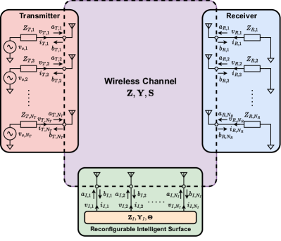
Figure 1: Multiport model of an RIS-aided communication system.

II Multiport Network Analysis

We consider a multiple-input multiple-output (MIMO) communication system aided by an RIS, where there are $N_{T}$ antennas at the transmitter, $N_{R}$ antennas at the receiver, and $N_{I}$ antennas at the RIS, as represented in Fig. 1. As in [25], we model the wireless channel as an $N$-port network, with $N=N_{T}+N_{I}+N_{R}$. According to the multiport network analysis [43, Chapter 4], this $N$-port network can be characterized by using its impedance, admittance, or scattering matrix, as described in the following.

II-A Modeling Based on the Impedance Parameters

The $N$-port network modeling the wireless channel can be characterized by its impedance matrix $\mathbf{Z}\in\mathbb{C}^{N\times N}$, such that

$$\mathbf{v}=\mathbf{Z}\mathbf{i},$$ (1)

where $\mathbf{v}\in\mathbb{C}^{N\times 1}$ and $\mathbf{i}\in\mathbb{C}^{N\times 1}$ are the voltages and currents at the $N$ ports, respectively. We can partition $\mathbf{v}$, $\mathbf{i}$, and $\mathbf{Z}$ as

$$\mathbf{v}=\begin{bmatrix}\mathbf{v}_{T}\\ \mathbf{v}_{I}\\ \mathbf{v}_{R}\end{bmatrix},\;\mathbf{i}=\begin{bmatrix}\mathbf{i}_{T}\\ \mathbf{i}_{I}\\ \mathbf{i}_{R}\end{bmatrix},\;\mathbf{Z}=\begin{bmatrix}\mathbf{Z}_{TT}&\mathbf{Z}_{TI}&\mathbf{Z}_{TR}\\ \mathbf{Z}_{IT}&\mathbf{Z}_{II}&\mathbf{Z}_{IR}\\ \mathbf{Z}_{RT}&\mathbf{Z}_{RI}&\mathbf{Z}_{RR}\end{bmatrix},$$ (2)

where $\mathbf{v}_{i}\in\mathbb{C}^{N_{i}\times 1}$ and $\mathbf{i}_{i}\in\mathbb{C}^{N_{i}\times 1}$ for $i\in\{T,I,R\}$ refer to the voltages and currents at the antennas of the transmitter, RIS, and receiver, respectively. Accordingly, $\mathbf{Z}_{TT}\in\mathbb{C}^{N_{T}\times N_{T}}$, $\mathbf{Z}_{II}\in\mathbb{C}^{N_{I}\times N_{I}}$, and $\mathbf{Z}_{RR}\in\mathbb{C}^{N_{R}\times N_{R}}$ refer to the impedance matrices of the antenna arrays at the transmitter, RIS, and receiver, respectively. The diagonal entries of $\mathbf{Z}_{TT}$, $\mathbf{Z}_{II}$, and $\mathbf{Z}_{RR}$ refer to the antenna self-impedance while the off-diagonal entries refer to antenna mutual coupling. $\mathbf{Z}_{RT}\in\mathbb{C}^{N_{R}\times N_{T}}$, $\mathbf{Z}_{IT}\in\mathbb{C}^{N_{I}\times N_{T}}$, and $\mathbf{Z}_{RI}\in\mathbb{C}^{N_{R}\times N_{I}}$ refer to the transmission impedance matrices from the transmitter to receiver, from the transmitter to the RIS, and from the RIS to the receiver, respectively.

At the transmitter, the $n_{T}$th antenna is connected in series with a source voltage $v_{s,n_{T}}$ and a source impedance $Z_{T,n_{T}}$, for $n_{T}=1,\ldots,N_{T}$. Therefore, $\mathbf{v}_{T}$ and $\mathbf{i}_{T}$ are related by

$$\mathbf{v}_{T}=\mathbf{v}_{s,T}-\mathbf{Z}_{T}\mathbf{i}_{T},$$ (3)

where $\mathbf{v}_{s,T}=[v_{s,1},v_{s,2},\ldots,v_{s,N_{T}}]^{T}\in\mathbb{C}^{N_{T}\times 1}$ refers to the source voltage vector and $\mathbf{Z}_{T}\in\mathbb{C}^{N_{T}\times N_{T}}$ is a diagonal matrix given by $\mathbf{Z}_{T}=\textrm{diag}(Z_{T,1},Z_{T,2},\ldots,Z_{T,N_{T}})$. At the RIS, the $N_{I}$ antennas are connected to an $N_{I}$-port reconfigurable impedance network and $\mathbf{v}_{I}$ is related to $\mathbf{i}_{I}$ by

$$\mathbf{v}_{I}=-\mathbf{Z}_{I}\mathbf{i}_{I},$$ (4)

where $\mathbf{Z}_{I}\in\mathbb{C}^{N_{I}\times N_{I}}$ is the impedance matrix of the $N_{I}$-port reconfigurable impedance network. At the receiver, the $n_{R}$th antenna is connected in series with a load impedance $Z_{R,n_{R}}$, for $n_{R}=1,\ldots,N_{R}$. Therefore, $\mathbf{v}_{R}$ and $\mathbf{i}_{R}$ are related by

$$\mathbf{v}_{R}=-\mathbf{Z}_{R}\mathbf{i}_{R},$$ (5)

where $\mathbf{Z}_{R}\in\mathbb{C}^{N_{R}\times N_{R}}$ is a diagonal matrix given by $\mathbf{Z}_{R}=\textrm{diag}(Z_{R,1},Z_{R,2},\ldots,Z_{R,N_{R}})$.

II-B Modeling Based on the Admittance Parameters

The wireless channel can also be characterized by its admittance matrix $\mathbf{Y}\in\mathbb{C}^{N\times N}$, with $\mathbf{Y}=\mathbf{Z}^{-1}$, such that

$$\mathbf{i}=\mathbf{Y}\mathbf{v}.$$ (6)

Similar to $\mathbf{Z}$, also $\mathbf{Y}$ can be partitioned as

$$\mathbf{Y}=\begin{bmatrix}\mathbf{Y}_{TT}&\mathbf{Y}_{TI}&\mathbf{Y}_{TR}\\ \mathbf{Y}_{IT}&\mathbf{Y}_{II}&\mathbf{Y}_{IR}\\ \mathbf{Y}_{RT}&\mathbf{Y}_{RI}&\mathbf{Y}_{RR}\end{bmatrix},$$ (7)

where $\mathbf{Y}_{ij}\in\mathbb{C}^{N_{i}\times N_{j}}$ for $i,j\in\{T,I,R\}$.

At the transmitter, $\mathbf{v}_{T}$ and $\mathbf{i}_{T}$ are related by

$$\mathbf{i}_{T}=\mathbf{i}_{s,T}-\mathbf{Y}_{T}\mathbf{v}_{T},$$ (8)

where $\mathbf{i}_{s,T}\in\mathbb{C}^{N_{T}\times 1}$ refers to the source current vector and $\mathbf{Y}_{T}\in\mathbb{C}^{N_{T}\times N_{T}}$ is a diagonal matrix given by $\mathbf{Y}_{T}=\mathbf{Z}_{T}^{-1}$. At the RIS, $\mathbf{v}_{I}$ and $\mathbf{i}_{I}$ are related by

$$\mathbf{i}_{I}=-\mathbf{Y}_{I}\mathbf{v}_{I},$$ (9)

where $\mathbf{Y}_{I}\in\mathbb{C}^{N_{I}\times N_{I}}$ is the admittance matrix of the $N_{I}$-port reconfigurable impedance network, given by $\mathbf{Y}_{I}=\mathbf{Z}_{I}^{-1}$. At the receiver, $\mathbf{v}_{R}$ and $\mathbf{i}_{R}$ are related by

$$\mathbf{i}_{R}=-\mathbf{Y}_{R}\mathbf{v}_{R},$$ (10)

where $\mathbf{Y}_{R}\in\mathbb{C}^{N_{R}\times N_{R}}$ is diagonal given by $\mathbf{Y}_{R}=\mathbf{Z}_{R}^{-1}$.

II-C Modeling Based on the Scattering Parameters

Finally, the wireless channel can be characterized by its scattering matrix $\mathbf{S}\in\mathbb{C}^{N\times N}$, so that we have

$$\mathbf{b}=\mathbf{S}\mathbf{a},$$ (11)

where $\mathbf{a}\in\mathbb{C}^{N\times 1}$ and $\mathbf{b}\in\mathbb{C}^{N\times 1}$ are the incident and reflected waves at the ports, respectively. We partition $\mathbf{a}$, $\mathbf{b}$, and $\mathbf{S}$ as

$$\mathbf{a}=\begin{bmatrix}\mathbf{a}_{T}\\ \mathbf{a}_{I}\\ \mathbf{a}_{R}\end{bmatrix},\;\mathbf{b}=\begin{bmatrix}\mathbf{b}_{T}\\ \mathbf{b}_{I}\\ \mathbf{b}_{R}\end{bmatrix},\;\mathbf{S}=\begin{bmatrix}\mathbf{S}_{TT}&\mathbf{S}_{TI}&\mathbf{S}_{TR}\\ \mathbf{S}_{IT}&\mathbf{S}_{II}&\mathbf{S}_{IR}\\ \mathbf{S}_{RT}&\mathbf{S}_{RI}&\mathbf{S}_{RR}\end{bmatrix},$$ (12)

where $\mathbf{a}_{i}\in\mathbb{C}^{N_{i}\times 1}$ and $\mathbf{b}_{i}\in\mathbb{C}^{N_{i}\times 1}$ for $i\in\{T,I,R\}$ refer to the incident and reflected waves at the antennas of the transmitter, RIS, and receiver, respectively, and $\mathbf{S}_{ij}\in\mathbb{C}^{N_{i}\times N_{j}}$ for $i,j\in\{T,I,R\}$. Remarkably, according to [43, Chapter 4], the vectors $\mathbf{v}$ and $\mathbf{i}$ are related to $\mathbf{a}$ and $\mathbf{b}$ though

$$\mathbf{v}=\mathbf{a}+\mathbf{b},\;\mathbf{i}=\frac{\mathbf{a}-\mathbf{b}}{Z_{0}}=Y_{0}\left(\mathbf{a}-\mathbf{b}\right),$$ (13)

respectively, where $Z_{0}$ is the characteristic impedance used to compute the $S$-parameters, typically set as $Z_{0}=50$ $\Omega$, and $Y_{0}=1/Z_{0}$ is the characteristic admittance. In addition, the matrix $\mathbf{S}$ can be expressed as a function of $\mathbf{Z}$ as

$$\mathbf{S}=\left(\mathbf{Z}+Z_{0}\mathbf{I}\right)^{-1}\left(\mathbf{Z}-Z_{0}\mathbf{I}\right).$$ (14)

At the transmitter, $\mathbf{a}_{T}$ and $\mathbf{b}_{T}$ are related by

$$\mathbf{a}_{T}=\mathbf{b}_{s,T}+\mathbf{\Gamma}_{T}\mathbf{b}_{T},$$ (15)

where $\mathbf{b}_{s,T}\in\mathbb{C}^{N_{T}\times 1}$ refers to the source wave vector and $\mathbf{\Gamma}_{T}\in\mathbb{C}^{N_{T}\times N_{T}}$ is diagonal with its $(n_{T},n_{T})$th element being the reflection coefficient of the $n_{T}$th source impedance, i.e.,

$$\mathbf{\Gamma}_{T}=\left(\mathbf{Z}_{T}+Z_{0}\mathbf{I}\right)^{-1}\left(\mathbf{Z}_{T}-Z_{0}\mathbf{I}\right).$$ (16)

At the RIS, $\mathbf{a}_{I}$ and $\mathbf{b}_{I}$ are related by

$$\mathbf{a}_{I}=\boldsymbol{\Theta}\mathbf{b}_{I},$$ (17)

where $\boldsymbol{\Theta}\in\mathbb{C}^{N_{I}\times N_{I}}$ denotes the scattering matrix of the $N_{I}$-port reconfigurable impedance network, written as

$$\boldsymbol{\Theta}=\left(\mathbf{Z}_{I}+Z_{0}\mathbf{I}\right)^{-1}\left(\mathbf{Z}_{I}-Z_{0}\mathbf{I}\right).$$ (18)

At the receiver, $\mathbf{a}_{R}$ and $\mathbf{b}_{R}$ are related by

$$\mathbf{a}_{R}=\mathbf{\Gamma}_{R}\mathbf{b}_{R},$$ (19)

where $\mathbf{\Gamma}_{R}\in\mathbb{C}^{N_{R}\times N_{R}}$ is diagonal with its $(n_{R},n_{R})$th element being the reflection coefficient of the $n_{R}$th load, i.e.,

$$\mathbf{\Gamma}_{R}=\left(\mathbf{Z}_{R}+Z_{0}\mathbf{I}\right)^{-1}\left(\mathbf{Z}_{R}-Z_{0}\mathbf{I}\right).$$ (20)

III General RIS-Aided Communication Model

We have characterized the relationships between the electrical properties at the transmitter, RIS, and receiver of an RIS-aided communication system. In this section, we determine the channel $\mathbf{H}\in\mathbb{C}^{N_{R}\times N_{T}}$ relating the voltage vector at the transmitter (transmitted signal) $\mathbf{v}_{T}$ and the voltage vector at the receiver (received signal) $\mathbf{v}_{R}$ through $\mathbf{v}_{R}=\mathbf{H}\mathbf{v}_{T}$. To this end, we introduce a universal framework enabling three equivalent analyses, based on $Z$-, $Y$-, and $S$-parameters.

III-A Universal Framework

Consider the following mathematical problem. Given two variable vectors $\mathbf{x}\in\mathbb{C}^{N\times 1}$ and $\mathbf{y}\in\mathbb{C}^{N\times 1}$, and a constant matrix $\mathbf{A}\in\mathbb{C}^{N\times N}$, respectively partitioned as

$$\mathbf{x}=\begin{bmatrix}\mathbf{x}_{1}\\ \mathbf{x}_{2}\\ \mathbf{x}_{3}\end{bmatrix},\;\mathbf{y}=\begin{bmatrix}\mathbf{y}_{1}\\ \mathbf{y}_{2}\\ \mathbf{y}_{3}\end{bmatrix},\;\mathbf{A}=\begin{bmatrix}\mathbf{A}_{11}&\mathbf{A}_{12}&\mathbf{A}_{13}\\ \mathbf{A}_{21}&\mathbf{A}_{22}&\mathbf{A}_{23}\\ \mathbf{A}_{31}&\mathbf{A}_{32}&\mathbf{A}_{33}\end{bmatrix},$$ (21)

where $\mathbf{x}_{i}\in\mathbb{C}^{N_{i}\times 1}$, $\mathbf{y}_{i}\in\mathbb{C}^{N_{i}\times 1}$, $\mathbf{A}_{ij}\in\mathbb{C}^{N_{i}\times N_{j}}$ for $i,j\in\{1,2,3\}$, and $N_{1}+N_{2}+N_{3}=N$, our goal is to solve

$$\begin{cases}\mathbf{y}=\mathbf{A}\mathbf{x},\\ \mathbf{x}_{1}=\mathbf{c}_{1}+\mathbf{A}_{1}\mathbf{y}_{1},\\ \mathbf{x}_{2}=\mathbf{A}_{2}\mathbf{y}_{2},\\ \mathbf{x}_{3}=\mathbf{A}_{3}\mathbf{y}_{3},\end{cases}$$ (22)

where $\mathbf{c}_{1}\in\mathbb{C}^{N_{1}\times 1}$ and $\mathbf{A}_{i}\in\mathbb{C}^{N_{i}\times N_{i}}$ for $i\in\{1,2,3\}$ are constant. In other words, we want to characterize the two variable vectors $\mathbf{x}$ and $\mathbf{y}$ as functions of the constants $\mathbf{A}$, $\mathbf{c}_{1}$, $\mathbf{A}_{1}$, $\mathbf{A}_{2}$, and $\mathbf{A}_{3}$. Remarkably, system (22) provides a universal framework that can be used to describe the equations of the multiport network analysis based on $Z$-, $Y$-, and $S$-parameters. In Tab. I, we report the relationship between the variables in this framework and the quantities in the three different parameters introduced in Section II.

TABLE I: Relationship between the universal framework
and the $Z$-, $Y$-, and $S$-parameters.

Framework	$Z$-parameters	$Y$-parameters	$S$-parameters
$\mathbf{x}$	$\mathbf{v}$	$\mathbf{i}$	$\mathbf{a}$
$\mathbf{y}$	$\mathbf{i}$	$\mathbf{v}$	$\mathbf{b}$
$\mathbf{A}$	$\mathbf{Z}^{-1}$	$\mathbf{Y}^{-1}$	$\mathbf{S}$
$\mathbf{c}_{1}$	$\mathbf{v}_{s,T}$	$\mathbf{i}_{s,T}$	$\mathbf{b}_{s,T}$
$\mathbf{A}_{1}$	$-\mathbf{Z}_{T}$	$-\mathbf{Y}_{T}$	$\mathbf{\Gamma}_{T}$
$\mathbf{A}_{2}$	$-\mathbf{Z}_{I}$	$-\mathbf{Y}_{I}$	$\boldsymbol{\Theta}$
$\mathbf{A}_{3}$	$-\mathbf{Z}_{R}$	$-\mathbf{Y}_{R}$	$\mathbf{\Gamma}_{R}$

To solve system (22), we rewrite it in a compact form

$$\begin{cases}\mathbf{y}=\mathbf{A}\mathbf{x},\\ \mathbf{x}=\mathbf{c}+\overline{\mathbf{A}}\mathbf{y},\end{cases}$$ (23)

where we introduce $\mathbf{c}\in\mathbb{C}^{N\times 1}$ and $\overline{\mathbf{A}}\in\mathbb{C}^{N\times N}$ as

$$\mathbf{c}=\begin{bmatrix}\mathbf{c}_{1}\\ \mathbf{0}\\ \mathbf{0}\end{bmatrix},\;\overline{\mathbf{A}}=\begin{bmatrix}\mathbf{A}_{1}&\mathbf{0}&\mathbf{0}\\ \mathbf{0}&\mathbf{A}_{2}&\mathbf{0}\\ \mathbf{0}&\mathbf{0}&\mathbf{A}_{3}\end{bmatrix}.$$ (24)

System (23) can be solved by noting that

$$\mathbf{x}=\mathbf{c}+\overline{\mathbf{A}}\mathbf{A}\mathbf{x},$$ (25)

gives

$$\mathbf{x}=\left(\mathbf{I}-\overline{\mathbf{A}}\mathbf{A}\right)^{-1}\mathbf{c}.$$ (26)

Thus, by introducing $\widetilde{\mathbf{A}}=\left(\mathbf{I}-\overline{\mathbf{A}}\mathbf{A}\right)^{-1}$, partitioned as

$$\widetilde{\mathbf{A}}=\begin{bmatrix}\widetilde{\mathbf{A}}_{11}&\widetilde{\mathbf{A}}_{12}&\widetilde{\mathbf{A}}_{13}\\ \widetilde{\mathbf{A}}_{21}&\widetilde{\mathbf{A}}_{22}&\widetilde{\mathbf{A}}_{23}\\ \widetilde{\mathbf{A}}_{31}&\widetilde{\mathbf{A}}_{32}&\widetilde{\mathbf{A}}_{33}\end{bmatrix},$$ (27)

we have

$$\mathbf{x}_{1}=\widetilde{\mathbf{A}}_{11}\mathbf{c}_{1},\;\mathbf{x}_{2}=\widetilde{\mathbf{A}}_{21}\mathbf{c}_{1},\;\mathbf{x}_{3}=\widetilde{\mathbf{A}}_{31}\mathbf{c}_{1},$$ (28)

providing an expression for the vector $\mathbf{x}$. Given $\mathbf{x}$, the vector $\mathbf{y}$ is determined by applying $\mathbf{y}=\mathbf{A}\mathbf{x}$ and system (22) is solved.

III-B Impedance Parameters Analysis

With the $Z$-parameters, the channel $\mathbf{H}$ is derived by solving the system of the four linear equations (1), (3), (4), and (5). According to Sec. III-A, this system gives

$$\mathbf{v}=\left(\mathbf{I}+\overline{\mathbf{Z}}\mathbf{Z}^{-1}\right)^{-1}\mathbf{v}_{s},$$ (29)

where we define $\mathbf{v}_{s}\in\mathbb{C}^{N\times 1}$ and $\overline{\mathbf{Z}}\in\mathbb{C}^{N\times N}$ as

$$\mathbf{v}_{s}=\begin{bmatrix}\mathbf{v}_{s,T}\\ \mathbf{0}\\ \mathbf{0}\end{bmatrix},\;\overline{\mathbf{Z}}=\begin{bmatrix}\mathbf{Z}_{T}&\mathbf{0}&\mathbf{0}\\ \mathbf{0}&\mathbf{Z}_{I}&\mathbf{0}\\ \mathbf{0}&\mathbf{0}&\mathbf{Z}_{R}\end{bmatrix}.$$ (30)

Thus, by introducing $\widetilde{\mathbf{Z}}=\left(\mathbf{I}+\overline{\mathbf{Z}}\mathbf{Z}^{-1}\right)^{-1}$, partitioned as

$$\widetilde{\mathbf{Z}}=\begin{bmatrix}\widetilde{\mathbf{Z}}_{TT}&\widetilde{\mathbf{Z}}_{TI}&\widetilde{\mathbf{Z}}_{TR}\\ \widetilde{\mathbf{Z}}_{IT}&\widetilde{\mathbf{Z}}_{II}&\widetilde{\mathbf{Z}}_{IR}\\ \widetilde{\mathbf{Z}}_{RT}&\widetilde{\mathbf{Z}}_{RI}&\widetilde{\mathbf{Z}}_{RR}\end{bmatrix},$$ (31)

we have

$$\mathbf{v}_{T}=\widetilde{\mathbf{Z}}_{TT}\mathbf{v}_{s,T},\;\mathbf{v}_{R}=\widetilde{\mathbf{Z}}_{RT}\mathbf{v}_{s,T}.$$ (32)

As a consequence of (32), we obtain

$$\mathbf{v}_{R}=\widetilde{\mathbf{Z}}_{RT}\mathbf{v}_{s,T}=\widetilde{\mathbf{Z}}_{RT}\widetilde{\mathbf{Z}}_{TT}^{-1}\mathbf{v}_{T},$$ (33)

yielding

$$\mathbf{H}=\widetilde{\mathbf{Z}}_{RT}\widetilde{\mathbf{Z}}_{TT}^{-1},$$ (34)

which is the general channel model based on the $Z$-parameters.

III-C Admittance Parameters Analysis

With the $Y$-parameters, the channel $\mathbf{H}$ is derived by solving the system of the four linear equations (6), (8), (9), and (10). According to Sec. III-A, this system gives

$$\mathbf{i}=\left(\mathbf{I}+\overline{\mathbf{Y}}\mathbf{Y}^{-1}\right)^{-1}\mathbf{i}_{s},$$ (35)

where we define $\mathbf{i}_{s}\in\mathbb{C}^{N\times 1}$ and $\overline{\mathbf{Y}}\in\mathbb{C}^{N\times N}$ as

$$\mathbf{i}_{s}=\begin{bmatrix}\mathbf{i}_{s,T}\\ \mathbf{0}\\ \mathbf{0}\end{bmatrix},\;\overline{\mathbf{Y}}=\begin{bmatrix}\mathbf{Y}_{T}&\mathbf{0}&\mathbf{0}\\ \mathbf{0}&\mathbf{Y}_{I}&\mathbf{0}\\ \mathbf{0}&\mathbf{0}&\mathbf{Y}_{R}\end{bmatrix}.$$ (36)

Thus, by introducing $\widetilde{\mathbf{Y}}=\left(\mathbf{I}+\overline{\mathbf{Y}}\mathbf{Y}^{-1}\right)^{-1}$, partitioned as

$$\widetilde{\mathbf{Y}}=\begin{bmatrix}\widetilde{\mathbf{Y}}_{TT}&\widetilde{\mathbf{Y}}_{TI}&\widetilde{\mathbf{Y}}_{TR}\\ \widetilde{\mathbf{Y}}_{IT}&\widetilde{\mathbf{Y}}_{II}&\widetilde{\mathbf{Y}}_{IR}\\ \widetilde{\mathbf{Y}}_{RT}&\widetilde{\mathbf{Y}}_{RI}&\widetilde{\mathbf{Y}}_{RR}\end{bmatrix},$$ (37)

we have

$$\mathbf{i}_{T}=\widetilde{\mathbf{Y}}_{TT}\mathbf{i}_{s,T},\;\mathbf{i}_{R}=\widetilde{\mathbf{Y}}_{RT}\mathbf{i}_{s,T}.$$ (38)

As a consequence of (8), (10), and (38), we obtain

$$\mathbf{v}_{R} =-\mathbf{Y}_{R}^{-1}\mathbf{i}_{R}=-\mathbf{Y}_{R}^{-1}\widetilde{\mathbf{Y}}_{RT}\mathbf{i}_{s,T}$$ (39)

$$=\mathbf{Y}_{R}^{-1}\widetilde{\mathbf{Y}}_{RT}\left(\widetilde{\mathbf{Y}}_{TT}-\mathbf{I}\right)^{-1}\mathbf{Y}_{T}\mathbf{v}_{T},$$ (40)

yielding

$$\mathbf{H}=\mathbf{Y}_{R}^{-1}\widetilde{\mathbf{Y}}_{RT}\left(\widetilde{\mathbf{Y}}_{TT}-\mathbf{I}\right)^{-1}\mathbf{Y}_{T},$$ (41)

which is the general channel model with the $Y$-parameters.

III-D Scattering Parameters Analysis

With the $S$-parameters, the channel $\mathbf{H}$ is derived by solving the system of (11), (15), (17), and (19). According to Sec. III-A, and using $\mathbf{b}=\mathbf{S}\mathbf{a}$, this system gives

$$\mathbf{b}=\mathbf{S}\left(\mathbf{I}-\mathbf{\Gamma}\mathbf{S}\right)^{-1}\mathbf{b}_{s},$$ (42)

where we define $\mathbf{b}_{s}\in\mathbb{C}^{N\times 1}$ and $\mathbf{\Gamma}\in\mathbb{C}^{N\times N}$ as

$$\mathbf{b}_{s}=\begin{bmatrix}\mathbf{b}_{s,T}\\ \mathbf{0}\\ \mathbf{0}\end{bmatrix},\;\mathbf{\Gamma}=\begin{bmatrix}\mathbf{\Gamma}_{T}&\mathbf{0}&\mathbf{0}\\ \mathbf{0}&\boldsymbol{\Theta}&\mathbf{0}\\ \mathbf{0}&\mathbf{0}&\mathbf{\Gamma}_{R}\end{bmatrix}.$$ (43)

Thus, by introducing $\widetilde{\mathbf{S}}=\mathbf{S}\left(\mathbf{I}-\mathbf{\Gamma}\mathbf{S}\right)^{-1}$, partitioned as

$$\widetilde{\mathbf{S}}=\begin{bmatrix}\widetilde{\mathbf{S}}_{TT}&\widetilde{\mathbf{S}}_{TI}&\widetilde{\mathbf{S}}_{TR}\\ \widetilde{\mathbf{S}}_{IT}&\widetilde{\mathbf{S}}_{II}&\widetilde{\mathbf{S}}_{IR}\\ \widetilde{\mathbf{S}}_{RT}&\widetilde{\mathbf{S}}_{RI}&\widetilde{\mathbf{S}}_{RR}\end{bmatrix},$$ (44)

we have

$$\mathbf{b}_{T}=\widetilde{\mathbf{S}}_{TT}\mathbf{b}_{s,T},\;\mathbf{b}_{R}=\widetilde{\mathbf{S}}_{RT}\mathbf{b}_{s,T}.$$ (45)

As a consequence of (13), (15), (19), and (45), we obtain

$$\mathbf{v}_{R} =\mathbf{a}_{R}+\mathbf{b}_{R}=\left(\mathbf{\Gamma}_{R}+\mathbf{I}\right)\widetilde{\mathbf{S}}_{RT}\mathbf{b}_{s,T}$$ (46)

$$=\left(\mathbf{\Gamma}_{R}+\mathbf{I}\right)\widetilde{\mathbf{S}}_{RT}\left(\mathbf{I}+\mathbf{\Gamma}_{T}\widetilde{\mathbf{S}}_{TT}+\widetilde{\mathbf{S}}_{TT}\right)^{-1}\mathbf{v}_{T},$$ (47)

yielding

$$\mathbf{H}=\left(\mathbf{\Gamma}_{R}+\mathbf{I}\right)\widetilde{\mathbf{S}}_{RT}\left(\mathbf{I}+\mathbf{\Gamma}_{T}\widetilde{\mathbf{S}}_{TT}+\widetilde{\mathbf{S}}_{TT}\right)^{-1},$$ (48)

which is the general channel model based on the $S$-parameters, in agreement with [25].

III-E Equivalence Between General Models

We have derived three general channel models in (34), (41), and (48), based on $Z$-, $Y$-, and $S$-parameters, respectively. We now confirm, for the first time, that these channel models are equivalent representations of a RIS-aided system.

For this purpose, it is necessary to relate the vectors $\mathbf{i}_{s,T}$ and $\mathbf{b}_{s,T}$ to the vector $\mathbf{v}_{s,T}$ by observing that (3), (8), and (15) are three equivalent descriptions of the electrical properties at the transmitter. By equating (3) and (8), and recalling that $\mathbf{Y}_{T}=\mathbf{Z}_{T}^{-1}$, we obtain

$$\mathbf{i}_{s,T}=\mathbf{Y}_{T}\mathbf{v}_{s,T},$$ (49)

giving the relationship between $\mathbf{i}_{s,T}$ and $\mathbf{v}_{s,T}$. In addition, by equating (3) and (15), and using (13) and (16), we obtain

$$\mathbf{b}_{s,T}=\frac{\mathbf{I}-\mathbf{\Gamma}_{T}}{2}\mathbf{v}_{s,T},$$ (50)

giving the relationship between $\mathbf{b}_{s,T}$ and $\mathbf{v}_{s,T}$.

We first show that the general channel model based on the $Z$-parameters (34) is equivalent to the general channel model based on the $Y$-parameters (41). To this end, we note that (34) is a direct consequence of (29) and that (41) is a direct consequence of (35). Thus, it is convenient to just show that (29) and (35) are equivalent. By using $\overline{\mathbf{Z}}=\overline{\mathbf{Y}}^{-1}$ and $\mathbf{Z}=\mathbf{Y}^{-1}$, we can rewrite (29) as

$$\mathbf{v}=\left(\mathbf{I}+\overline{\mathbf{Y}}^{-1}\mathbf{Y}\right)^{-1}\mathbf{v}_{s}.$$ (51)

Then, recalling that $\mathbf{i}=\mathbf{Y}\mathbf{v}$ and observing that (49) gives $\mathbf{v}_{s}=\overline{\mathbf{Y}}^{-1}\mathbf{i}_{s}$, from (51) we obtain

$$\mathbf{i} =\mathbf{Y}\left(\mathbf{I}+\overline{\mathbf{Y}}^{-1}\mathbf{Y}\right)^{-1}\overline{\mathbf{Y}}^{-1}\mathbf{i}_{s}$$ (52)

$$=\left(\mathbf{I}+\overline{\mathbf{Y}}\mathbf{Y}^{-1}\right)^{-1}\mathbf{i}_{s},$$ (53)

giving (35). Thus, we have that the general channel models (34) and (41) are equivalent since they are a direct consequence of equivalent equations.

We now show that the general channel model based on the $Z$-parameters (34) is also equivalent to the general channel model based on the $S$-parameters (48). Since (34) is a direct consequence of (29) and (48) is a direct consequence of (42), it is convenient to just show that (29) and (42) are equivalent. By using $\overline{\mathbf{Z}}=Z_{0}\left(\mathbf{I}+\mathbf{\Gamma}\right)\left(\mathbf{I}-\mathbf{\Gamma}\right)^{-1}$ and $\mathbf{Z}=Z_{0}\left(\mathbf{I}+\mathbf{S}\right)\left(\mathbf{I}-\mathbf{S}\right)^{-1}$, we can rewrite (29) as

$$\mathbf{v} =\left(\mathbf{I}+\left(\mathbf{I}+\mathbf{\Gamma}\right)\left(\mathbf{I}-\mathbf{\Gamma}\right)^{-1}\left(\mathbf{I}-\mathbf{S}\right)\left(\mathbf{I}+\mathbf{S}\right)^{-1}\right)^{-1}\mathbf{v}_{s}$$ (54)

$$=\left(\mathbf{I}+\mathbf{S}\right)\left(\mathbf{I}-\mathbf{\Gamma}\mathbf{S}\right)^{-1}\left(\mathbf{I}-\mathbf{\Gamma}\right)\mathbf{v}_{s}/2.$$ (55)

Then, recalling that $\mathbf{b}=(\mathbf{S}^{-1}+\mathbf{I})^{-1}\mathbf{v}$ and observing that (50) gives $\mathbf{v}_{s}=2(\mathbf{I}-\mathbf{\Gamma})^{-1}\mathbf{b}_{s}$, from (55) we obtain

$$\mathbf{b} =\left(\mathbf{S}^{-1}+\mathbf{I}\right)^{-1}\left(\mathbf{I}+\mathbf{S}\right)\left(\mathbf{I}-\mathbf{\Gamma}\mathbf{S}\right)^{-1}\mathbf{b}_{s}$$ (56)

$$=\mathbf{S}\left(\mathbf{I}-\mathbf{\Gamma}\mathbf{S}\right)^{-1}\mathbf{b}_{s},$$ (57)

giving (42). Thus, the general channel models (34) and (48) are equivalent since they are a direct consequence of equivalent equations, in agreement with microwave theory [43, Chapter 4]. By the transitive property of the equivalence relation, we also have that the general channel models based on the $Y$- and $S$-parameters are equivalent.

IV RIS-Aided Communication Model with Unilateral Approximation

We have derived three general channel models based on the $Z$-, $Y$-, and $S$-parameters. They account for imperfect matching and mutual coupling at the transmitter, RIS, and receiver as they have been obtained without any approximation or assumption. However, it is difficult to obtain insights into the role of the RIS in the communication model due to the presence of matrix inversion operations. To gain a better understanding of the communication models, in this section, we approximate the general models by assuming sufficiently large transmission distances.

IV-A Universal Framework

We begin by simplifying the universal framework introduced in Sec. III-A. Specifically, we consider the matrix $\mathbf{A}$ to be block lower triangular given by

$$\mathbf{A}=\begin{bmatrix}\mathbf{A}_{11}&\mathbf{0}&\mathbf{0}\\ \mathbf{A}_{21}&\mathbf{A}_{22}&\mathbf{0}\\ \mathbf{A}_{31}&\mathbf{A}_{32}&\mathbf{A}_{33}\end{bmatrix}.$$ (58)

Remarkably, system (22) with $\mathbf{A}$ given by (58) provides a universal framework that can be used to describe the equations based on $Z$-, $Y$-, and $S$-parameters with the unilateral approximation [42], as it will be clarified in Sec. IV-B, IV-C, and IV-D, respectively. With the simplification in (58), the solution to system (22) given by (28) simplifies as

$$\mathbf{x}_{1}=\left(\mathbf{I}-\mathbf{A}_{1}\mathbf{A}_{11}\right)^{-1}\mathbf{c}_{1},$$ (59)

$$\mathbf{x}_{2}=\left(\mathbf{I}-\mathbf{A}_{2}\mathbf{A}_{22}\right)^{-1}\mathbf{A}_{2}\mathbf{A}_{21}\left(\mathbf{I}-\mathbf{A}_{1}\mathbf{A}_{11}\right)^{-1}\mathbf{c}_{1},$$ (60)

$$\mathbf{x}_{3}=\left(\mathbf{A}_{3}^{-1}-\mathbf{A}_{33}\right)^{-1}\left(\mathbf{A}_{31}+\mathbf{A}_{32}\left(\mathbf{A}_{2}^{-1}-\mathbf{A}_{22}\right)^{-1}\mathbf{A}_{21}\right)\\ \times\left(\mathbf{I}-\mathbf{A}_{1}\mathbf{A}_{11}\right)^{-1}\mathbf{c}_{1},$$ (61)

allowing to explicitly express $\mathbf{x}$ in terms of $\mathbf{A}$, $\mathbf{c}_{1}$, $\mathbf{A}_{1}$, $\mathbf{A}_{2}$, and $\mathbf{A}_{3}$. In the following, we use this universal framework to derive the channel model based on $Z$-, $Y$-, and $S$-parameters.

IV-B Impedance Parameters Analysis

To simplify (34), we observe that with a large transmission distance between a transmitter and a receiver, the electrical properties at the transmitter are approximately independent of the electrical properties at the receiver. The minimum transmission distance at which this phenomenon occurs is a function of the number of antennas at the transmitter and receiver, their radiation pattern, and the antenna spacing, as discussed in [42]. Thus, assuming that the transmission distance is large enough, we can consider the so-called unilateral approximation and set $\mathbf{Z}_{TI}=\mathbf{0}$, $\mathbf{Z}_{TR}=\mathbf{0}$, and $\mathbf{Z}_{IR}=\mathbf{0}$ [42]. Note that with this approximation we do not assume the wireless channel to be non-reciprocal. Conversely, we set to zero the upper block triangular part of $\mathbf{Z}$ as it does not impact the expression of $\mathbf{H}$. Thus, we can express $\mathbf{v}_{T}$ and $\mathbf{v}_{R}$ as

$$\mathbf{v}_{T}=\left(\mathbf{I}+\mathbf{Z}_{T}\mathbf{Z}_{TT}^{-1}\right)^{-1}\mathbf{v}_{s,T},$$ (62)

$$\mathbf{v}_{R}=\mathbf{Z}_{R}\left(\mathbf{Z}_{R}+\mathbf{Z}_{RR}\right)^{-1}\left(\mathbf{Z}_{RT}-\mathbf{Z}_{RI}\left(\mathbf{Z}_{I}+\mathbf{Z}_{II}\right)^{-1}\mathbf{Z}_{IT}\right)\\ \times\left(\mathbf{Z}_{T}+\mathbf{Z}_{TT}\right)^{-1}\mathbf{v}_{s,T},$$ (63)

according to Sec. IV-A. Consequently, the channel model based on the $Z$-parameters is given by

$$\mathbf{H}=\mathbf{Z}_{R}\left(\mathbf{Z}_{R}+\mathbf{Z}_{RR}\right)^{-1}\\ \times\left(\mathbf{Z}_{RT}-\mathbf{Z}_{RI}\left(\mathbf{Z}_{I}+\mathbf{Z}_{II}\right)^{-1}\mathbf{Z}_{IT}\right)\mathbf{Z}_{TT}^{-1},$$ (64)

explicitly clarifying the impact of $\mathbf{Z}$, $\mathbf{Z}_{T}$, $\mathbf{Z}_{I}$, and $\mathbf{Z}_{R}$, in agreement with [40, Corollary 1].

IV-C Admittance Parameters Analysis

As discussed for the $Z$-parameters, we can also simplify (41) by considering the unilateral approximation. Setting $\mathbf{Z}_{TI}=\mathbf{0}$, $\mathbf{Z}_{TR}=\mathbf{0}$, and $\mathbf{Z}_{IR}=\mathbf{0}$, and recalling that the entire matrix $\mathbf{Y}$ is related to $\mathbf{Z}$ through $\mathbf{Y}=\mathbf{Z}^{-1}$, we obtain $\mathbf{Y}_{TI}=\mathbf{0}$, $\mathbf{Y}_{TR}=\mathbf{0}$, and $\mathbf{Y}_{IR}=\mathbf{0}$, allowing us to express $\mathbf{i}_{T}$ and $\mathbf{i}_{R}$ as

$$\mathbf{i}_{T}=\left(\mathbf{I}+\mathbf{Y}_{T}\mathbf{Y}_{TT}^{-1}\right)^{-1}\mathbf{i}_{s,T},$$ (65)

$$\mathbf{i}_{R}=\mathbf{Y}_{R}\left(\mathbf{Y}_{R}+\mathbf{Y}_{RR}\right)^{-1}\Bigl{(}\mathbf{Y}_{RT}\Bigr{.}\\ \left.-\mathbf{Y}_{RI}\left(\mathbf{Y}_{I}+\mathbf{Y}_{II}\right)^{-1}\mathbf{Y}_{IT}\right)\left(\mathbf{Y}_{T}+\mathbf{Y}_{TT}\right)^{-1}\mathbf{i}_{s,T},$$ (66)

according to Sec. IV-A. Thus, the channel model based on the $Y$-parameters with the unilateral approximation is given by

$$\mathbf{H}=\left(\mathbf{Y}_{R}+\mathbf{Y}_{RR}\right)^{-1}\left(-\mathbf{Y}_{RT}+\mathbf{Y}_{RI}\left(\mathbf{Y}_{I}+\mathbf{Y}_{II}\right)^{-1}\mathbf{Y}_{IT}\right),$$ (67)

explicitly defining the effect of $\mathbf{Y}$, $\mathbf{Y}_{T}$, $\mathbf{Y}_{I}$, and $\mathbf{Y}_{R}$.

IV-D Scattering Parameters Analysis

As done for the $Z$- and $Y$-parameters, we simplify (48) by considering the unilateral approximation to better understand the role of the RIS. Setting $\mathbf{Z}_{TI}=\mathbf{0}$, $\mathbf{Z}_{TR}=\mathbf{0}$, and $\mathbf{Z}_{IR}=\mathbf{0}$, and recalling (14), we obtain $\mathbf{S}_{TI}=\mathbf{0}$, $\mathbf{S}_{TR}=\mathbf{0}$, and $\mathbf{S}_{IR}=\mathbf{0}$, which allow us to express $\mathbf{b}_{T}$ and $\mathbf{b}_{R}$ as

$$\mathbf{b}_{T}=\mathbf{S}_{TT}\left(\mathbf{I}-\mathbf{\Gamma}_{T}\mathbf{S}_{TT}\right)^{-1}\mathbf{b}_{s,T},$$ (68)

$$\mathbf{b}_{R}=\left(\mathbf{I}-\mathbf{S}_{RR}\mathbf{\Gamma}_{R}\right)^{-1}\left(\mathbf{S}_{RT}+\mathbf{S}_{RI}\left(\mathbf{I}-\boldsymbol{\Theta}\mathbf{S}_{II}\right)^{-1}\boldsymbol{\Theta}\mathbf{S}_{IT}\right)\\ \times\left(\mathbf{I}-\mathbf{\Gamma}_{T}\mathbf{S}_{TT}\right)^{-1}\mathbf{b}_{s,T},$$ (69)

according to Sec. IV-A. Thus, the channel model based on the $S$-parameters with the unilateral approximation is given by

$$\mathbf{H}=\left(\mathbf{\Gamma}_{R}+\mathbf{I}\right)\left(\mathbf{I}-\mathbf{S}_{RR}\mathbf{\Gamma}_{R}\right)^{-1}\\ \times\left(\mathbf{S}_{RT}+\mathbf{S}_{RI}\left(\mathbf{I}-\boldsymbol{\Theta}\mathbf{S}_{II}\right)^{-1}\boldsymbol{\Theta}\mathbf{S}_{IT}\right)\left(\mathbf{I}+\mathbf{S}_{TT}\right)^{-1},$$ (70)

clearly highlighting the role of $\mathbf{S}$, $\mathbf{\Gamma}_{T}$, $\boldsymbol{\Theta}$, and $\mathbf{\Gamma}_{R}$.

Remarkably, the three models (64), (67), and (70) effectively show the impact of $\mathbf{Z}_{I}$, $\mathbf{Y}_{I}$, and $\boldsymbol{\Theta}$ on the communication, while still capturing the impact of imperfect matching and mutual coupling at the transmitter, RIS, and receiver.

IV-E Mappings Between Parameters

Under the unilateral approximation, we can derive simplified mappings that allow us to express the $Y$- and $S$-parameters as functions of $Z$-parameters.

IV-E1 From $Z$- to $Y$-Parameters

To express the matrices $\mathbf{Y}_{RT}$, $\mathbf{Y}_{RI}$, and $\mathbf{Y}_{IT}$ as functions of $\mathbf{Z}$, we consider the relationship $\mathbf{Y}=\mathbf{Z}^{-1}$ where $\mathbf{Z}$ has been simplified through the unilateral approximation, i.e., $\mathbf{Z}_{TI}=\mathbf{0}$, $\mathbf{Z}_{TR}=\mathbf{0}$, and $\mathbf{Z}_{IR}=\mathbf{0}$. Thus, by computing $\mathbf{Y}$, we have

$$\mathbf{Y}_{RI}=-\mathbf{Z}_{RR}^{-1}\mathbf{Z}_{RI}\mathbf{Z}_{II}^{-1},\;\mathbf{Y}_{IT}=-\mathbf{Z}_{II}^{-1}\mathbf{Z}_{IT}\mathbf{Z}_{TT}^{-1},$$ (71)

$$\mathbf{Y}_{RT}=\mathbf{Z}_{RR}^{-1}\left(-\mathbf{Z}_{RT}+\mathbf{Z}_{RI}\mathbf{Z}_{II}^{-1}\mathbf{Z}_{IT}\right)\mathbf{Z}_{TT}^{-1}.$$ (72)

IV-E2 From $Z$- to $S$-Parameters

To express the matrices $\mathbf{S}_{RT}$, $\mathbf{S}_{RI}$, and $\mathbf{S}_{IT}$ as functions of $\mathbf{Z}$, we consider the relationship (14) where $\mathbf{Z}_{TI}=\mathbf{0}$, $\mathbf{Z}_{TR}=\mathbf{0}$, and $\mathbf{Z}_{IR}=\mathbf{0}$. Thus, it can be proved that

$$\mathbf{S}_{RI}=2Z_{0}\left(\mathbf{Z}_{RR}+Z_{0}\mathbf{I}\right)^{-1}\mathbf{Z}_{RI}\left(\mathbf{Z}_{II}+Z_{0}\mathbf{I}\right)^{-1},$$ (73)

$$\mathbf{S}_{IT}=2Z_{0}\left(\mathbf{Z}_{II}+Z_{0}\mathbf{I}\right)^{-1}\mathbf{Z}_{IT}\left(\mathbf{Z}_{TT}+Z_{0}\mathbf{I}\right)^{-1},$$ (74)

$$\mathbf{S}_{RT}=2Z_{0}\left(\mathbf{Z}_{RR}+Z_{0}\mathbf{I}\right)^{-1}\Bigl{(}\mathbf{Z}_{RT}\Bigr{.}\\ \left.-\mathbf{Z}_{RI}\left(\mathbf{Z}_{II}+Z_{0}\mathbf{I}\right)^{-1}\mathbf{Z}_{IT}\right)\left(\mathbf{Z}_{TT}+Z_{0}\mathbf{I}\right)^{-1}.$$ (75)

Interestingly, these mappings further clarify the equivalence of the three analyses and the meaning of the different terms. In the following, we show that these mappings play a fundamental role in relating the EM-compliant models derived in this study with the channel model widely used in related literature.

TABLE II: Channel models based on $Z$-, $Y$-, and $S$-parameters with corresponding assumptions and approximations.

	$Z$-parameters	$Y$-parameters	$S$-parameters
Channel model	$\widetilde{\mathbf{Z}}_{RT}\widetilde{\mathbf{Z}}_{TT}^{-1}$	$\mathbf{Y}_{R}^{-1}\widetilde{\mathbf{Y}}_{RT}\left(\widetilde{\mathbf{Y}}_{TT}-\mathbf{I}\right)^{-1}\mathbf{Y}_{T}$	$\left(\mathbf{\Gamma}_{R}+\mathbf{I}\right)\widetilde{\mathbf{S}}_{RT}\left(\mathbf{I}+\mathbf{\Gamma}_{T}\widetilde{\mathbf{S}}_{TT}+\widetilde{\mathbf{S}}_{TT}\right)^{-1}$
A1: Sufficiently large transmission distances⋆	$\mathbf{Z}_{TI}=\mathbf{0}$, $\mathbf{Z}_{TR}=\mathbf{0}$, $\mathbf{Z}_{IR}=\mathbf{0}$	$\mathbf{Y}_{TI}=\mathbf{0}$, $\mathbf{Y}_{TR}=\mathbf{0}$, $\mathbf{Y}_{IR}=\mathbf{0}$	$\mathbf{S}_{TI}=\mathbf{0}$, $\mathbf{S}_{TR}=\mathbf{0}$, $\mathbf{S}_{IR}=\mathbf{0}$
Channel model with A1	$\mathbf{Z}_{R}\left(\mathbf{Z}_{R}+\mathbf{Z}_{RR}\right)^{-1}\left(\mathbf{Z}_{RT}-\mathbf{Z}_{RI}\left(\mathbf{Z}_{I}+\mathbf{Z}_{II}\right)^{-1}\mathbf{Z}_{IT}\right)\mathbf{Z}_{TT}^{-1}$	$\left(\mathbf{Y}_{R}+\mathbf{Y}_{RR}\right)^{-1}\left(-\mathbf{Y}_{RT}+\mathbf{Y}_{RI}\left(\mathbf{Y}_{I}+\mathbf{Y}_{II}\right)^{-1}\mathbf{Y}_{IT}\right)$	$\left(\mathbf{\Gamma}_{R}+\mathbf{I}\right)\left(\mathbf{I}-\mathbf{S}_{RR}\mathbf{\Gamma}_{R}\right)^{-1}\left(\mathbf{S}_{RT}+\mathbf{S}_{RI}\left(\mathbf{I}-\boldsymbol{\Theta}\mathbf{S}_{II}\right)^{-1}\boldsymbol{\Theta}\mathbf{S}_{IT}\right)\left(\mathbf{I}+\mathbf{S}_{TT}\right)^{-1}$
A2: Perfect matching and no mutual coupling at TX and RX	$\mathbf{Z}_{TT}=Z_{0}\mathbf{I}$, $\mathbf{Z}_{RR}=Z_{0}\mathbf{I}$	$\mathbf{Y}_{TT}=Y_{0}\mathbf{I}$, $\mathbf{Y}_{RR}=Y_{0}\mathbf{I}$	$\mathbf{S}_{TT}=\mathbf{0}$, $\mathbf{S}_{RR}=\mathbf{0}$
A3: Impedances at TX and RX equal to $Z_{0}$	$\mathbf{Z}_{T}=Z_{0}\mathbf{I}$, $\mathbf{Z}_{R}=Z_{0}\mathbf{I}$	$\mathbf{Y}_{T}=Y_{0}\mathbf{I}$, $\mathbf{Y}_{R}=Y_{0}\mathbf{I}$	$\mathbf{\Gamma}_{T}=\mathbf{0}$, $\mathbf{\Gamma}_{R}=\mathbf{0}$
Channel model with A1, A2, and A3	$\frac{1}{2Z_{0}}\left(\mathbf{Z}_{RT}-\mathbf{Z}_{RI}\left(\mathbf{Z}_{I}+\mathbf{Z}_{II}\right)^{-1}\mathbf{Z}_{IT}\right)$	$\frac{1}{2Y_{0}}\left(-\mathbf{Y}_{RT}+\mathbf{Y}_{RI}\left(\mathbf{Y}_{I}+\mathbf{Y}_{II}\right)^{-1}\mathbf{Y}_{IT}\right)$	$\mathbf{S}_{RT}+\mathbf{S}_{RI}\left(\mathbf{I}-\boldsymbol{\Theta}\mathbf{S}_{II}\right)^{-1}\boldsymbol{\Theta}\mathbf{S}_{IT}$
A4: Perfect matching and no mutual coupling at RIS	$\mathbf{Z}_{II}=Z_{0}\mathbf{I}$	$\mathbf{Y}_{II}=Y_{0}\mathbf{I}$	$\mathbf{S}_{II}=\mathbf{0}$
Channel model with A1, A2, A3, and A4	$\frac{1}{2Z_{0}}\left(\mathbf{Z}_{RT}-\mathbf{Z}_{RI}\left(\mathbf{Z}_{I}+Z_{0}\mathbf{I}\right)^{-1}\mathbf{Z}_{IT}\right)$	$\frac{1}{2Y_{0}}\left(-\mathbf{Y}_{RT}+\mathbf{Y}_{RI}\left(\mathbf{Y}_{I}+Y_{0}\mathbf{I}\right)^{-1}\mathbf{Y}_{IT}\right)$	$\mathbf{S}_{RT}+\mathbf{S}_{RI}\boldsymbol{\Theta}\mathbf{S}_{IT}$

^⋆ Distances larger than the critical distance provided in [42].

V RIS-Aided Communication Model with Perfect Matching and No Mutual Coupling

We have derived three general channel models based on the $Z$-, $Y$-, and $S$-parameters, and we have simplified them by considering the unilateral approximation. In this section, we further simplify the obtained models to gain engineering insights into the role of the RIS in the communication system.

V-A Impedance Parameters Analysis

To further simplify (64), we consider two assumptions in addition to the unilateral approximation. First, we assume that the antennas at the transmitter and receiver are perfectly matched and have no mutual coupling, yielding $\mathbf{Z}_{TT}=Z_{0}\mathbf{I}$ and $\mathbf{Z}_{RR}=Z_{0}\mathbf{I}$. Second, we assume that the impedances at the transmitter $Z_{T,n_{T}}$ and the receiver $Z_{R,n_{R}}$ are all $Z_{0}$, i.e., $\mathbf{Z}_{T}=Z_{0}\mathbf{I}$ and $\mathbf{Z}_{R}=Z_{0}\mathbf{I}$. With these assumptions, the channel model (64) simplifies to

$$\mathbf{H}=\frac{1}{2Z_{0}}\left(\mathbf{Z}_{RT}-\mathbf{Z}_{RI}\left(\mathbf{Z}_{I}+\mathbf{Z}_{II}\right)^{-1}\mathbf{Z}_{IT}\right).$$ (76)

In addition, assuming perfect matching and no mutual coupling at the RIS, i.e., $\mathbf{Z}_{II}=Z_{0}\mathbf{I}$, we obtain

$$\mathbf{H}=\frac{1}{2Z_{0}}\left(\mathbf{Z}_{RT}-\mathbf{Z}_{RI}\left(\mathbf{Z}_{I}+Z_{0}\mathbf{I}\right)^{-1}\mathbf{Z}_{IT}\right),$$ (77)

giving the simplified channel model based on the $Z$-parameters with perfect matching and no mutual coupling. By further assuming the RIS elements to be canonical minimum scattering antennas [44], the channel without the RIS is equivalent to the channel when the RIS elements are open-circuited, i.e., $\mathbf{Z}_{I}=\infty\mathbf{I}$, given by $\mathbf{H}=\mathbf{Z}_{RT}/(2Z_{0})$ following (77).

V-B Admittance Parameters Analysis

To further simplify (67), we consider the two additional assumptions as discussed for the $Z$-parameters. First, assuming perfect matching and no mutual coupling at the transmitter and receiver, and noting that, with the unilateral approximation, the relationship $\mathbf{Y}=\mathbf{Z}^{-1}$ implies $\mathbf{Y}_{ii}=\mathbf{Z}_{ii}^{-1}$, for $i\in\{T,I,R\}$, we obtain $\mathbf{Y}_{TT}=Y_{0}\mathbf{I}$ and $\mathbf{Y}_{RR}=Y_{0}\mathbf{I}$. Second, considering all the impedances at the transmitter and receiver to be $Z_{0}$, and recalling that $\mathbf{Y}_{T}=\mathbf{Z}_{T}^{-1}$ and $\mathbf{Y}_{R}=\mathbf{Z}_{R}^{-1}$, we have $\mathbf{Y}_{T}=Y_{0}\mathbf{I}$ and $\mathbf{Y}_{R}=Y_{0}\mathbf{I}$. With these assumptions, the channel model (67) simplifies to

$$\mathbf{H}=\frac{1}{2Y_{0}}\left(-\mathbf{Y}_{RT}+\mathbf{Y}_{RI}\left(\mathbf{Y}_{I}+\mathbf{Y}_{II}\right)^{-1}\mathbf{Y}_{IT}\right),$$ (78)

In addition, assuming perfect matching and no mutual coupling at the RIS, i.e., $\mathbf{Y}_{II}=Y_{0}\mathbf{I}$, we obtain

$$\mathbf{H}=\frac{1}{2Y_{0}}\left(-\mathbf{Y}_{RT}+\mathbf{Y}_{RI}\left(\mathbf{Y}_{I}+Y_{0}\mathbf{I}\right)^{-1}\mathbf{Y}_{IT}\right),$$ (79)

giving the simplified channel model based on the $Y$-parameters with perfect matching and no mutual coupling.

V-C Scattering Parameters Analysis

As done for $Z$- and $Y$-parameters, we now further simplify (70). First, assuming perfect matching and no mutual coupling at the transmitter and receiver, and noting that, with the unilateral approximation, (14) implies $\mathbf{S}_{ii}=\left(\mathbf{Z}_{ii}+Z_{0}\mathbf{I}\right)^{-1}\left(\mathbf{Z}_{ii}-Z_{0}\mathbf{I}\right)$, for $i\in\{T,I,R\}$, we obtain $\mathbf{S}_{TT}=\mathbf{0}$ and $\mathbf{S}_{RR}=\mathbf{0}$. Second, considering all the impedances at the transmitter and receiver to be $Z_{0}$, and recalling (16) and (20), we have $\mathbf{\Gamma}_{T}=\mathbf{0}$ and $\mathbf{\Gamma}_{R}=\mathbf{0}$. With these two assumptions, (70) simplifies to

$$\mathbf{H}=\mathbf{S}_{RT}+\mathbf{S}_{RI}\left(\mathbf{I}-\boldsymbol{\Theta}\mathbf{S}_{II}\right)^{-1}\boldsymbol{\Theta}\mathbf{S}_{IT}.$$ (80)

In addition, assuming perfect matching and no mutual coupling at the RIS, i.e., $\mathbf{S}_{II}=\mathbf{0}$, we obtain

$$\mathbf{H}=\mathbf{S}_{RT}+\mathbf{S}_{RI}\boldsymbol{\Theta}\mathbf{S}_{IT},$$ (81)

which is the simplified channel model based on $S$-parameters with perfect matching and no mutual coupling, commonly used in communications in agreement with [25]. We summarize the main results of the three analyses based on $Z$-, $Y$-, and $S$-parameters in Tab. II.

V-D Mappings Between Parameters

Under the assumptions of perfect matching and no mutual coupling, we can derive more simplified mappings that allow us to express the $Y$- and $S$-parameters as functions of $Z$-parameters. By using such mappings, it is possible to directly show that the simplified channel models (77), (79), and (81) are equivalent.

V-D1 From $Z$- to $Y$-Parameters

Considering the unilateral approximation and perfect matching and no mutual coupling at the transmitter and receiver, the matrices $\mathbf{Y}_{RT}$, $\mathbf{Y}_{RI}$, and $\mathbf{Y}_{IT}$ can be expressed as functions of $\mathbf{Z}$ by setting $\mathbf{Z}_{TT}=Z_{0}\mathbf{I}$ and $\mathbf{Z}_{RR}=Z_{0}\mathbf{I}$ in (71) and (72), yielding

$$\mathbf{Y}_{RI}=-\frac{\mathbf{Z}_{RI}\mathbf{Z}_{II}^{-1}}{Z_{0}},\;\mathbf{Y}_{IT}=-\frac{\mathbf{Z}_{II}^{-1}\mathbf{Z}_{IT}}{Z_{0}},$$ (82)

$$\mathbf{Y}_{RT}=\frac{1}{Z_{0}^{2}}\left(-\mathbf{Z}_{RT}+\mathbf{Z}_{RI}\mathbf{Z}_{II}^{-1}\mathbf{Z}_{IT}\right).$$ (83)

In addition, with perfect matching and no mutual coupling at the RIS, i.e., $\mathbf{Z}_{II}=Z_{0}\mathbf{I}$, (82) and (83) boil down to

$$\mathbf{Y}_{RI}=-\frac{\mathbf{Z}_{RI}}{Z_{0}^{2}},\;\mathbf{Y}_{IT}=-\frac{\mathbf{Z}_{IT}}{Z_{0}^{2}},$$ (84)

$$\mathbf{Y}_{RT}=\frac{1}{Z_{0}^{2}}\left(-\mathbf{Z}_{RT}+\frac{\mathbf{Z}_{RI}\mathbf{Z}_{IT}}{Z_{0}}\right).$$ (85)

Interestingly, by substituting $\mathbf{Y}_{I}=\mathbf{Z}_{I}^{-1}$, (84), and (85) into (79), we directly obtain (77), confirming that the two analyses based on $Z$- and $Y$-parameters lead to the same result.

V-D2 From $Z$- to $S$-Parameters

To express the matrices $\mathbf{S}_{RT}$, $\mathbf{S}_{RI}$, and $\mathbf{S}_{IT}$ as functions of $\mathbf{Z}$ with the unilateral approximation and perfect matching and no mutual coupling at the transmitter and receiver, we can set $\mathbf{Z}_{TT}=Z_{0}\mathbf{I}$ and $\mathbf{Z}_{RR}=Z_{0}\mathbf{I}$ in (73), (74), and (75), yielding

$$\mathbf{S}_{RI}=\mathbf{Z}_{RI}\left(\mathbf{Z}_{II}+Z_{0}\mathbf{I}\right)^{-1},\;\mathbf{S}_{IT}=\left(\mathbf{Z}_{II}+Z_{0}\mathbf{I}\right)^{-1}\mathbf{Z}_{IT},$$ (86)

$$\mathbf{S}_{RT}=\frac{1}{2Z_{0}}\left(\mathbf{Z}_{RT}-\mathbf{Z}_{RI}\left(\mathbf{Z}_{II}+Z_{0}\mathbf{I}\right)^{-1}\mathbf{Z}_{IT}\right).$$ (87)

In addition, with perfect matching and no mutual coupling at the RIS, i.e., $\mathbf{Z}_{II}=Z_{0}\mathbf{I}$, (86) and (87) boil down to

$$\mathbf{S}_{RI}=\frac{\mathbf{Z}_{RI}}{2Z_{0}},\;\mathbf{S}_{IT}=\frac{\mathbf{Z}_{IT}}{2Z_{0}},$$ (88)

$$\mathbf{S}_{RT}=\frac{1}{2Z_{0}}\left(\mathbf{Z}_{RT}-\frac{\mathbf{Z}_{RI}\mathbf{Z}_{IT}}{2Z_{0}}\right).$$ (89)

Interestingly, by substituting (18), (88), and (89) into (81), we directly obtain (77), confirming that the two analyses based on the $Z$- and $S$-parameters lead to the same conclusion.

V-E Relationship with the Widely Used Model

We have derived three equivalent simplified channel models under the assumptions of perfect matching and no mutual coupling. In this section, we relate these models with the RIS-aided channel model widely used in related literature.

In RIS literature [3]-[38], the notation

$$\mathbf{H}_{RT}=\mathbf{S}_{RT},\;\mathbf{H}_{RI}=\mathbf{S}_{RI},\;\mathbf{H}_{IT}=\mathbf{S}_{IT},$$ (90)

is commonly used to denote the channel matrices from the transmitter to the receiver, from the RIS to the receiver, and from the transmitter to the RIS, respectively. By substituting (90) into the simplified channel based on the $S$-parameters (81), we obtain

$$\mathbf{H}=\mathbf{H}_{RT}+\mathbf{H}_{RI}\boldsymbol{\Theta}\mathbf{H}_{IT},$$ (91)

which is the RIS-aided communication model widely used in related literature. Thus, we can conclude that the widely used model (91) is derived by considering the unilateral approximation and under the assumptions of perfect matching and no mutual coupling, in agreement with [25].

An interesting aspect of the channel model (91) is the dependence of $\mathbf{H}_{RT}$ on $\mathbf{H}_{RI}$ and $\mathbf{H}_{IT}$ as a result of (88), (89), and (90). However, this aspect is commonly neglected in related literature, where it is implicitly considered

$$\mathbf{S}_{RT}\approx\frac{\mathbf{Z}_{RT}}{2Z_{0}},$$ (92)

as an approximation of (89). Remarkably, (92) can be obtained by considering the relationship

$$\mathbf{Z}=2Z_{0}\left(\mathbf{I}-\mathbf{S}\right)^{-1}-Z_{0}\mathbf{I},$$ (93)

which is derived from (14), by applying the first-order Neumann series approximation $\left(\mathbf{I}-\mathbf{S}\right)^{-1}\approx\left(\mathbf{I}+\mathbf{S}\right)$. With this approximation, from (93) we obtain $\mathbf{Z}\approx Z_{0}\left(\mathbf{I}+2\mathbf{S}\right)$, directly giving (92). Note that the first-order Neumann series approximation holds as long as $\|\mathbf{S}\|_{F}$ is small, which is typically valid in wireless communication scenarios given the high losses suffered from the propagating signal.

According to the approximation in (92), when the direct channel between transmitter and receiver is completely obstructed, i.e., $\mathbf{Z}_{RT}=\mathbf{0}$, we have $\mathbf{H}_{RT}=\mathbf{0}$, as widely accepted in related literature. However, according to (89), a completely obstructed direct channel, i.e., $\mathbf{Z}_{RT}=\mathbf{0}$, gives $\mathbf{H}_{RT}=-\mathbf{H}_{RI}\mathbf{H}_{IT}$, which is in general non zero, as correctly noticed in [21, 41]. The physical meaning of having $\mathbf{H}_{RT}\neq\mathbf{0}$ in the case of a completely obstructed direct channel, i.e., $\mathbf{Z}_{RT}=\mathbf{0}$, lies in the structural scattering of the RIS.

Since the approximation in (92) causes an inconsistency, especially when $\mathbf{Z}_{RT}=\mathbf{0}$, it is worth quantifying the difference between (91) and the channel model resulting from (92), widely used in the literature. To this end, we assume a completely obstructed direct channel, i.e., $\mathbf{Z}_{RT}=\mathbf{0}$, and consider a single-input single-output (SISO) system, i.e., $N_{R}=1$ and $N_{T}=1$, where (91) boils down to

$$h=-\mathbf{h}_{RI}\mathbf{h}_{IT}+\mathbf{h}_{RI}\boldsymbol{\Theta}\mathbf{h}_{IT},$$ (94)

and, considering the approximation in (92), to

$$h\approx\mathbf{h}_{RI}\boldsymbol{\Theta}\mathbf{h}_{IT}\triangleq h^{\prime}.$$ (95)

In the following, we derive the scaling laws of the received signal power achieved under the channel models in (94) and (95) when a conventional RIS architecture is considered.

As for the model in (94), the received signal power is given by $P_{R}=|-\mathbf{h}_{RI}\mathbf{h}_{IT}+\mathbf{h}_{RI}\boldsymbol{\Theta}\mathbf{h}_{IT}|^{2}$, where a unit transmit power is assumed with no loss of generality. Thus, the maximum received signal power is given by

$$P_{R}=\left(\left|\mathbf{h}_{RI}\mathbf{h}_{IT}\right|+\sum_{n_{I}=1}^{N_{I}}\left|\left[\mathbf{h}_{RI}\right]_{n_{I}}\left[\mathbf{h}_{IT}\right]_{n_{I}}\right|\right)^{2},$$ (96)

achievable by co-phasing the terms $-\mathbf{h}_{RI}\mathbf{h}_{IT}$ and $\mathbf{h}_{RI}\boldsymbol{\Theta}\mathbf{h}_{IT}$ through an appropriate phase shift introduced by $\boldsymbol{\Theta}$.

As for the widely used model $h^{\prime}$, the received signal power is equal to $P_{R}^{\prime}=|\mathbf{h}_{RI}\boldsymbol{\Theta}\mathbf{h}_{IT}|^{2}$. Thus, it is possible to optimize the RIS to achieve a received signal power of

$$P_{R}^{\prime}=\left(\sum_{n_{I}=1}^{N_{I}}\left|\left[\mathbf{h}_{RI}\right]_{n_{I}}\left[\mathbf{h}_{IT}\right]_{n_{I}}\right|\right)^{2}.$$ (97)

We define the relative difference between the average received signal power $\text{E}[P_{R}]$ and $\text{E}[P_{R}^{\prime}]$ as

$$\delta=\frac{\text{E}\left[P_{R}\right]-\text{E}\left[P_{R}^{\prime}\right]}{\text{E}\left[P_{R}\right]}.$$ (98)

To gain numerical insights into (98), we consider line-of-sight (LoS) channels given by $\mathbf{h}_{RI}=[e^{\phi_{1}},\ldots,e^{\phi_{N_{I}}}]$ and $\mathbf{h}_{IT}=[e^{\psi_{1}},\ldots,e^{\psi_{N_{I}}}]^{T}$. With these channels, in the case of the model $h$, we have

$$\text{E}\left[P_{R}\right]=\text{E}\left[\left|\mathbf{h}_{RI}\mathbf{h}_{IT}\right|^{2}\right]+N_{I}^{2}+2N_{I}\text{E}\left[\left|\mathbf{h}_{RI}\mathbf{h}_{IT}\right|\right].$$ (99)

Approximating the term $\mathbf{h}_{RI}\mathbf{h}_{IT}$ as a sum of $N_{I}$ independent and identically distributed (i.i.d.) random variables with mean $0$ and variance $1$, it holds $\mathbf{h}_{RI}\mathbf{h}_{IT}\sim\mathcal{CN}(0,N_{I})$ by the Central Limit Theorem. Thus, by using $\text{E}[|\mathbf{h}_{RI}\mathbf{h}_{IT}|]=\sqrt{\frac{\pi}{4}N_{I}}$ and $\text{E}[|\mathbf{h}_{RI}\mathbf{h}_{IT}|^{2}]=N_{I}$, we have

$$\text{E}\left[P_{R}\right]=N_{I}^{2}+\sqrt{\pi N_{I}}N_{I}+N_{I}.$$ (100)

Besides, in the case of the widely used model $h^{\prime}$, we have

$$\text{E}\left[P_{R}^{\prime}\right]=P_{R}^{\prime}=N_{I}^{2}.$$ (101)

Considering (100) and (101), the relative difference between $\text{E}[P_{R}]$ and $\text{E}[P_{R}^{\prime}]$ under LoS channels is equal to

$$\delta=\frac{\sqrt{\pi N_{I}}+1}{N_{I}+\sqrt{\pi N_{I}}+1},$$ (102)

giving $\delta\rightarrow 0$ for $N_{I}\rightarrow\infty$.

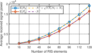
Figure 2: Average received signal power obtained with the model $h$ and the widely used model $h^{\prime}$.

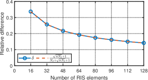
Figure 3: Relative difference between the average received signal power obtained with the model $h$ and the widely used model $h^{\prime}$.

TABLE III: Constraints of lossless and reciprocal RIS architectures based on $Z$-, $Y$-, and $S$-parameters.

	$Z$-parameters	$Y$-parameters	$S$-parameters
Single-connected	$\mathbf{Z}_{I}=\mathrm{diag}\left(Z_{1},\ldots,Z_{N_{I}}\right)$, $Z_{n_{I}}=jX_{n_{I}}$, $X_{n_{I}}\in\mathbb{R}$, $\forall n_{I}$	$\mathbf{Y}_{I}=\mathrm{diag}\left(Y_{1},\ldots,Y_{N_{I}}\right)$, $Y_{n_{I}}=jB_{n_{I}}$, $B_{n_{I}}\in\mathbb{R}$, $\forall n_{I}$	$\boldsymbol{\Theta}=\mathrm{diag}\left(\Theta_{1},\ldots,\Theta_{N_{I}}\right)$, $\Theta_{n_{I}}=e^{j\theta_{n_{I}}}$, $\theta_{n_{I}}\in[0,2\pi)$, $\forall n_{I}$
Fully-connected	$\mathbf{Z}_{I}=j\mathbf{X}_{I}$, $\mathbf{X}_{I}=\mathbf{X}_{I}^{T}$, $\mathbf{X}_{I}\in\mathbb{R}^{N_{I}\times N_{I}}$	$\mathbf{Y}_{I}=j\mathbf{B}_{I}$, $\mathbf{B}_{I}=\mathbf{B}_{I}^{T}$, $\mathbf{B}_{I}\in\mathbb{R}^{N_{I}\times N_{I}}$	$\boldsymbol{\Theta}^{H}\boldsymbol{\Theta}=\mathbf{I}$, $\boldsymbol{\Theta}=\boldsymbol{\Theta}^{T}$
Group-connected	$\mathbf{Z}_{I}=\mathrm{diag}\left(\mathbf{Z}_{I,1},\ldots,\mathbf{Z}_{I,G}\right)$, $\mathbf{Z}_{I,g}=j\mathbf{X}_{I,g}$, $\mathbf{X}_{I,g}=\mathbf{X}_{I,g}^{T}$, $\mathbf{X}_{I,g}\in\mathbb{R}^{N_{G}\times N_{G}}$, $\forall g$	$\mathbf{Y}_{I}=\mathrm{diag}\left(\mathbf{Y}_{I,1},\ldots,\mathbf{Y}_{I,G}\right)$, $\mathbf{Y}_{I,g}=j\mathbf{B}_{I,g}$, $\mathbf{B}_{I,g}=\mathbf{B}_{I,g}^{T}$, $\mathbf{B}_{I,g}\in\mathbb{R}^{N_{G}\times N_{G}}$, $\forall g$	$\boldsymbol{\Theta}=\mathrm{diag}\left(\boldsymbol{\Theta}_{1},\ldots,\boldsymbol{\Theta}_{G}\right)$, $\boldsymbol{\Theta}_{g}^{H}\boldsymbol{\Theta}_{g}=\mathbf{I}$, $\boldsymbol{\Theta}_{g}=\boldsymbol{\Theta}_{g}^{T}$, $\forall g$
Tree-connected⋆	$-$	$\mathbf{Y}_{I}=j\mathbf{B}_{I}$, $\mathbf{B}_{I}=\mathbf{B}_{I}^{T}$, $\mathbf{B}_{I}\in\mathbb{R}^{N_{I}\times N_{I}}$, $\left[\mathbf{B}_{I}\right]_{i,j}=0$ if $\left|i-j\right|>1$	$-$
Forest-connected⋆	$-$	$\mathbf{Y}_{I}=\mathrm{diag}\left(\mathbf{Y}_{I,1},\ldots,\mathbf{Y}_{I,G}\right)$, $\mathbf{Y}_{I,g}=j\mathbf{B}_{I,g}$, $\mathbf{B}_{I,g}=\mathbf{B}_{I,g}^{T}$, $\mathbf{B}_{I,g}\in\mathbb{R}^{N_{G}\times N_{G}}$, $\left[\mathbf{B}_{I,g}\right]_{i,j}=0$ if $\left|i-j\right|>1$, $\forall g$	$-$

^⋆ For these RIS families, the tridiagonal RIS architecture is considered [31], and the constraints cannot be expressed in terms of the $Z$- and $S$-parameters.

In Fig. 2, we report the average received signal power achieved with $h$ and the approximated model $h^{\prime}$. We observe that the received signal power for the channel $h$ is higher because of the additional term $-\mathbf{h}_{RI}\mathbf{h}_{IT}$. In addition, in Fig. 3, we report the relative difference between the average received signal power achieved with $h$ and with the approximated model $h^{\prime}$. We observe that, despite the difference vanishes when $N_{I}\rightarrow\infty$, it is non-negligible for a practical number of RIS elements since it vanishes slowly with $N_{I}$.

VI RIS Architectures and Optimization

We have shown that $Z$-, $Y$-, and $S$-parameters can be equivalently used to characterize the RIS-aided communication model. Similarly, they can be equivalently used to characterize the $N_{I}$-port reconfigurable impedance network implementing the RIS. In this section, we discuss how the matrices $\mathbf{Z}_{I}$, $\mathbf{Y}_{I}$, and $\boldsymbol{\Theta}$ can be used to characterize different RIS architectures, including conventional RIS and BD-RIS. In addition, we discuss the advantages of $Z$-, $Y$-, and $S$-parameters in optimizing the RIS.

VI-A RIS Architectures

In conventional RIS, also known as single-connected, each RIS port is solely connected to ground through a tunable impedance [25]. Hence, the resulting impedance, admittance, and scattering matrices are diagonal, as given in Tab. III, where $Z_{n_{I}}$ is the tunable impedance connecting the $n_{I}$th RIS port to ground, $Y_{n_{I}}=Z_{n_{I}}^{-1}$, and $\Theta_{n_{I}}$ is the reflection coefficient corresponding to $Z_{n_{I}}$, given by $\Theta_{n_{I}}=(Z_{n_{I}}-Z_{0})/(Z_{n_{I}}+Z_{0})$, according to (18), for $n_{I}=1,\ldots,N_{I}$. Furthermore, in the case of a lossless single-connected RIS, $Z_{n_{I}}$ and $Y_{n_{I}}$ are purely imaginary, and $|\Theta_{n_{I}}|=1$, for $n_{I}=1,\ldots,N_{I}$, as shown in Tab. III. This conventional circuit topology is the simplest RIS circuit topology, offering limited flexibility [25].

To overcome the limited flexibility of conventional RIS, the ports in BD-RIS can also be connected to each other through additional tunable impedance (or admittance) components. By denoting the tunable admittance connecting the $n_{I}$th port to the $m_{I}$th port as $Y_{n_{I},m_{I}}$, the $(n_{I},m_{I})$th entry of the admittance matrix is given by

$$\left[\mathbf{Y}_{I}\right]_{n_{I},m_{I}}=\begin{cases}-Y_{n_{I},m_{I}}&n_{I}\neq m_{I}\\ Y_{n_{I}}+\sum_{k\neq n_{I}}Y_{n_{I},k}&n_{I}=m_{I}\end{cases},$$ (103)

as discussed in [25]. Thus, the admittance matrix of BD-RIS is not limited to being diagonal. The same holds for the impedance and scattering matrices of BD-RIS, as it can be easily noticed by applying $\mathbf{Z}_{I}=\mathbf{Y}_{I}^{-1}$ and (18). Depending on the topology of the interconnections between the RIS ports, multiple RIS architectures have been proposed. In Tab. III, we report the constraint of fully-/group-connected RIS [25], and tree-/forest-connected RIS with the tridiagonal architecture [31] based on the three parameters. In group- and forest-connected RIS, the elements are grouped into $G$ groups, each with size $N_{G}=N/G$, such that $\mathbf{Z}_{I,g}\in\mathbb{C}^{N_{G}\times N_{G}}$, $\mathbf{Y}_{I,g}\in\mathbb{C}^{N_{G}\times N_{G}}$, and $\boldsymbol{\Theta}_{g}\in\mathbb{C}^{N_{G}\times N_{G}}$ are the impedance, admittance, and scattering matrix of the $g$th group, for $g=1,\ldots,G$, respectively [25, 31]. The $N_{I}$-port network of the RIS is often assumed to be reciprocal (not including non-reciprocal media) and lossless (to maximize the scattered power). If the RIS is reciprocal, the impedance, admittance, and scattering matrices are symmetric. Furthermore, if the RIS is lossless, the impedance and admittance matrices are purely imaginary while the scattering matrix is unitary, as shown in Tab. III.

VI-B RIS Optimization Based on the Impedance Parameters

Since $Z$-, $Y$-, and $S$-parameters can be used interchangeably to characterize the RIS architecture, we now highlight the advantages of using the different parameters to optimize the RIS. To this end, we consider three case studies derived from the received signal power maximization problem in an RIS-aided MIMO system. In this communication system, the transmitted signal is expressed as $\mathbf{v}_{T}=\mathbf{w}s$, where $\mathbf{w}\in\mathbb{C}^{N_{T}\times 1}$ is the normalized precoder subject to $\|\mathbf{w}\|=1$, and $s\in\mathbb{C}$ is the transmitted symbol with average power $P_{T}=\mathrm{E}[|s|^{2}]$. Besides, the signal used for detection is given by $z=\mathbf{g}\mathbf{v}_{R}\in\mathbb{C}$, where $\mathbf{g}\in\mathbb{C}^{1\times N_{R}}$ is the normalized combiner subject to the constraint $\|\mathbf{g}\|=1$, and $\mathbf{v}_{R}=\mathbf{H}\mathbf{v}_{T}$ is the received signal. Thus, the received signal power is given by $P_{R}=P_{T}|\mathbf{g}\mathbf{H}\mathbf{w}|^{2}$.

$Z$-parameters proved to be the effective representation when optimizing the RIS with mutual coupling [16]-[20]. Specifically, RIS characterized through the $Z$-parameters have been optimized by applying the Neumann series approximation [16]-[18], by iteratively optimizing the tunable loads in closed-form [19], and trough gradient ascent [20]. Furthermore, it has been shown that $Z$-parameters facilitate the optimization of BD-RIS in the presence of mutual coupling at the RIS [30].

As a case study, we consider the received signal power maximization problem in an RIS-aided system in the presence of mutual coupling, with the RIS being group-connected, including single- and fully-connected as two special cases [25]. Considering lossless and reciprocal RIS, i.e., with $\mathbf{Z}_{I}=j\mathbf{X}_{I}$ and $\mathbf{X}_{I}=\mathbf{X}_{I}^{T}$, where $\mathbf{X}_{I}$ is the RIS reactance matrix, and $\mathbf{H}$ given as in (76), our problem writes as

$$\underset{\mathbf{w},\mathbf{g},\mathbf{X}_{I}}{\mathsf{\mathrm{max}}}\;\; \frac{P_{T}}{4Z_{0}^{2}}\left|\mathbf{g}\left(\mathbf{Z}_{RT}-\mathbf{Z}_{RI}\left(j\mathbf{X}_{I}+\mathbf{Z}_{II}\right)^{-1}\mathbf{Z}_{IT}\right)\mathbf{w}\right|^{2}$$ (104)

$$\mathsf{\mathrm{s.t.}}\;\;\; \mathbf{X}_{I}=\mathrm{diag}\left(\mathbf{X}_{I,1},\ldots,\mathbf{X}_{I,G}\right),$$ (105)

$$\mathbf{X}_{I,g}=\mathbf{X}_{I,g}^{T},\;\forall g,$$ (106)

$$\left\|\mathbf{w}\right\|=1,\;\left\|\mathbf{g}\right\|=1,$$ (107)

which is solved by jointly optimizing $\mathbf{w}$, $\mathbf{g}$, and $\mathbf{X}_{I}$. To solve (104)-(107), we initialize $\mathbf{X}_{I}$ to a feasible value and alternate between the following two steps. First, with $\mathbf{X}_{I}$ fixed, $\mathbf{w}$ and $\mathbf{g}$ are updated as the dominant right and left singular vectors of $\mathbf{Z}_{RT}-\mathbf{Z}_{RI}(j\mathbf{X}_{I}+\mathbf{Z}_{II})^{-1}\mathbf{Z}_{IT}$, respectively, which is globally optimal. Second, with $\mathbf{w}$ and $\mathbf{g}$ fixed, $\mathbf{X}_{I}$ is updated by solving

$$\underset{\mathbf{X}_{I}}{\mathsf{\mathrm{max}}}\;\left|z_{RT}^{\text{eff}}-\mathbf{z}_{RI}^{\text{eff}}\left(j\mathbf{X}_{I}+\mathbf{Z}_{II}\right)^{-1}\mathbf{z}_{IT}^{\text{eff}}\right|^{2}\;\mathsf{\mathrm{s.t.}}\;\eqref{eq:PR-z-c1},\;\eqref{eq:PR-z-c2},$$ (108)

where $z_{RT}^{\text{eff}}=\mathbf{g}\mathbf{Z}_{RT}\mathbf{w}$, $\mathbf{z}_{RI}^{\text{eff}}=\mathbf{g}\mathbf{Z}_{RI}$, and $\mathbf{z}_{IT}^{\text{eff}}=\mathbf{Z}_{IT}\mathbf{w}$, as proposed in [30]. These two steps are alternatively repeated until convergence of the objective (104).

VI-C RIS Optimization Based on the Admittance Parameters

RIS optimization based on $Y$-parameters is necessary in the case of BD-RIS whose admittance matrix $\mathbf{Y}_{I}$ is sparse, i.e., there is only a limited number of tunable admittance components interconnecting the RIS elements, such as in tree- and forest-connected RISs [31]. In this case, $Y$-parameters are the effective representation since the entries of $\mathbf{Y}_{I}$ are directly linked to the tunable admittance components in the BD-RIS circuit topology, as given by (103).

As a case study, we consider the received signal power maximization problem in an RIS-aided system, with the RIS being forest-connected, including single- and tree-connected as two special cases [31]. Considering lossless and reciprocal RIS, i.e., with $\mathbf{Y}_{I}=j\mathbf{B}_{I}$ and $\mathbf{B}_{I}=\mathbf{B}_{I}^{T}$, where $\mathbf{B}_{I}$ is the RIS susceptance matrix, and $\mathbf{H}$ given as in (79), assuming no mutual coupling, our problem writes as

$$\underset{\mathbf{w},\mathbf{g},\mathbf{B}_{I}}{\mathsf{\mathrm{max}}}\;\; \frac{P_{T}}{4Y_{0}^{2}}\left|\mathbf{g}\left(-\mathbf{Y}_{RT}+\mathbf{Y}_{RI}\left(j\mathbf{B}_{I}+Y_{0}\mathbf{I}\right)^{-1}\mathbf{Y}_{IT}\right)\mathbf{w}\right|^{2}$$ (109)

$$\mathsf{\mathrm{s.t.}}\;\;\; \mathbf{B}_{I}=\mathrm{diag}\left(\mathbf{B}_{I,1},\ldots,\mathbf{B}_{I,G}\right),$$ (110)

$$\mathbf{B}_{I,g}=\mathbf{B}_{I,g}^{T},\>\left[\mathbf{B}_{I,g}\right]_{i,j}=0\textrm{ if }\left|i-j\right|>1,\forall g,$$ (111)

$$\left\|\mathbf{w}\right\|=1,\;\left\|\mathbf{g}\right\|=1,$$ (112)

where (111) indicates that the $g$th block of the susceptance matrix $\mathbf{B}_{g}$ has a tridiagonal architecture, as introduced in [31]. To jointly optimize $\mathbf{w}$, $\mathbf{g}$, and $\mathbf{B}_{I}$, we initialize $\mathbf{B}_{I}$ to a feasible value and alternate between the following two steps. First, with $\mathbf{B}_{I}$ fixed, $\mathbf{w}$ and $\mathbf{g}$ are updated as the dominant right and left singular vectors of $-\mathbf{Y}_{RT}+\mathbf{Y}_{RI}(j\mathbf{B}_{I}+Y_{0}\mathbf{I})^{-1}\mathbf{Y}_{IT}$, respectively, which is a global optimal solution. Second, with $\mathbf{w}$ and $\mathbf{g}$ fixed, $\mathbf{B}_{I}$ is updated by solving

$$\underset{\mathbf{B}_{I}}{\mathsf{\mathrm{max}}}\;\left|-y_{RT}^{\text{eff}}+\mathbf{y}_{RI}^{\text{eff}}\left(j\mathbf{B}_{I}+Y_{0}\mathbf{I}\right)^{-1}\mathbf{y}_{IT}^{\text{eff}}\right|^{2}\;\mathsf{\mathrm{s.t.}}\;\eqref{eq:PR-y-c1},\;\eqref{eq:PR-y-c2},$$ (113)

where $y_{RT}^{\text{eff}}=\mathbf{g}\mathbf{Y}_{RT}\mathbf{w}$, $\mathbf{y}_{RI}^{\text{eff}}=\mathbf{g}\mathbf{Y}_{RI}$, and $\mathbf{y}_{IT}^{\text{eff}}=\mathbf{Y}_{IT}\mathbf{w}$. Remarkably, (113) has been solved in [31], where a globally optimal solution for each block $\mathbf{B}_{I,g}$ has been proposed. These two steps are alternatively repeated until convergence of (109).

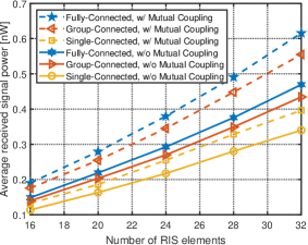
(a) $Z$-parameters, w/ and w/o mutual coupling.

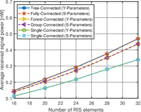
(b) $Y$- and $S$-parameters, w/o mutual coupling.

Figure 4: Average received signal power maximized using $Z$-, $Y$-, and $S$-parameters.

VI-D RIS Optimization Based on the Scattering Parameters

$S$-parameters have been commonly used to optimize conventional RIS in the vast majority of related works [3]-[15]. $S$-parameters own their popularity to the widely used channel model (81), in which $\boldsymbol{\Theta}=\mathrm{diag}\left(e^{j\theta_{1}},\ldots,e^{j\theta_{N_{I}}}\right)$ in the case of a lossless single-connected RIS. For single-connected RIS, $S$-parameters allow to directly optimize the phase shifts $\theta_{n_{I}}\in[0,2\pi)$ through several optimization techniques, including semidefinite relaxation (SDR) [3], iterative closed-form solutions [4], majorization-minimization (MM) and manifold optimization [5], alternating direction method of multipliers (ADMM) [13], and branch-and-bound (B&B) method [14]. For BD-RIS, the $S$-parameters enable the use of manifold optimization by exploiting the unitary constraint on $\boldsymbol{\Theta}$ [33]-[35]. In addition, the $S$-parameters allow for efficient optimization of BD-RIS by using tailored decompositions of $\boldsymbol{\Theta}$ [27], through symmetric unitary projection [28], and by solving the orthogonal Procrustes problem [36].

As a case study, we consider the received signal power maximization problem in an RIS-aided system, with the RIS being group-connected. Considering lossless and reciprocal RIS, i.e., with $\boldsymbol{\Theta}^{H}\boldsymbol{\Theta}=\mathbf{I}$ and $\boldsymbol{\Theta}=\boldsymbol{\Theta}^{T}$, and $\mathbf{H}$ given as in (81), assuming no mutual coupling, our problem writes as

$$\underset{\mathbf{w},\mathbf{g},\boldsymbol{\Theta}}{\mathsf{\mathrm{max}}}\;\; P_{T}\left|\mathbf{g}\left(\mathbf{S}_{RT}+\mathbf{S}_{RI}\boldsymbol{\Theta}\mathbf{S}_{IT}\right)\mathbf{w}\right|^{2}$$ (114)

$$\mathsf{\mathrm{s.t.}}\;\;\; \boldsymbol{\Theta}=\mathrm{diag}\left(\boldsymbol{\Theta}_{1},\ldots,\boldsymbol{\Theta}_{G}\right),$$ (115)

$$\boldsymbol{\Theta}_{g}=\boldsymbol{\Theta}_{g}^{T},\;\boldsymbol{\Theta}_{g}^{H}\boldsymbol{\Theta}_{g}=\mathbf{I},\;\forall g,$$ (116)

$$\left\|\mathbf{w}\right\|=1,\;\left\|\mathbf{g}\right\|=1,$$ (117)

which is solved by jointly optimizing $\mathbf{w}$, $\mathbf{g}$, and $\boldsymbol{\Theta}$. To this end, we initialize $\boldsymbol{\Theta}$ to a feasible value and alternate between the following two steps. First, with $\boldsymbol{\Theta}$ fixed, $\mathbf{w}$ and $\mathbf{g}$ are updated as the dominant right and left singular vectors of $\mathbf{S}_{RT}+\mathbf{S}_{RI}\boldsymbol{\Theta}\mathbf{S}_{IT}$, respectively, which is globally optimal. Second, with $\mathbf{w}$ and $\mathbf{g}$ fixed, $\boldsymbol{\Theta}$ is updated by solving

$$\underset{\boldsymbol{\Theta}}{\mathsf{\mathrm{max}}}\;\left|s_{RT}^{\text{eff}}+\mathbf{s}_{RI}^{\text{eff}}\boldsymbol{\Theta}\mathbf{s}_{IT}^{\text{eff}}\right|^{2}\;\mathsf{\mathrm{s.t.}}\;\eqref{eq:PR-s-c1},\;\eqref{eq:PR-s-c2},$$ (118)

where $s_{RT}^{\text{eff}}=\mathbf{g}\mathbf{S}_{RT}\mathbf{w}$, $\mathbf{s}_{RI}^{\text{eff}}=\mathbf{g}\mathbf{S}_{RI}$, and $\mathbf{s}_{IT}^{\text{eff}}=\mathbf{S}_{IT}\mathbf{w}$. Remarkably, (118) has been solved for group-connected RIS through a closed-form global optimally solution in [27]. These two steps are alternatively repeated until convergence of (114).

VII Numerical Results

In this section, we evaluate the performance obtained by solving the three optimization problems presented in Sec. VI, using $Z$-, $Y$-, and $S$-parameters. The transmitter, RIS, and receiver are located at $(0,0)$, $(50,2)$, and $(52,0)$ in meters (m), respectively. We set $N_{T}=2$ and $N_{R}=2$, and assume that the direct channel between the transmitter and receiver is completely obstructed, i.e., $\mathbf{Z}_{RT}=\mathbf{0}$. For the large-scale path loss of the channels from the RIS to the receiver and from the transmitter to the RIS, we use the distance-dependent path loss model $L_{ij}(d_{ij})=L_{0}d_{ij}^{-\alpha_{ij}}$, where $L_{0}$ is the reference path loss at distance 1 m, $d_{ij}$ is the distance, and $\alpha_{ij}$ is the path loss exponent, for $ij\in\{RI,IT\}$. We set $L_{0}=-30$ dB, $\alpha_{RI}=2.8$, $\alpha_{IT}=2$, and $P_{T}=10$ mW. For the small-scale fading, we model the channels as i.i.d. Rayleigh, i.e., $\mathbf{S}_{RI}\sim\mathcal{CN}(\mathbf{0},L_{RI}\mathbf{I})$ and $\mathbf{S}_{IT}\sim\mathcal{CN}(\mathbf{0},L_{IT}\mathbf{I})$. Given $\mathbf{Z}_{RT}$, $\mathbf{S}_{RI}$, and $\mathbf{S}_{IT}$, we obtain the rest of the off-diagonal blocks of $\mathbf{Z}$, $\mathbf{Y}$, and $\mathbf{S}$ through (84), (85), (88), and (89).

In Fig. 4, we report the average received signal power obtained by optimizing the RIS through $Z$-, $Y$-, and $S$-parameters. In the case of group- and forest-connected RISs, the group size is $N_{G}=4$. The schemes “w/o Mutual Coupling” are obtained by setting $\mathbf{Z}_{II}=Z_{0}\mathbf{I}$. Besides, the schemes “w/ Mutual Coupling” in Fig. 4(a) are obtained by modeling $\mathbf{Z}_{II}$ as follows: its diagonal entries are set to $Z_{0}$, assuming perfectly matched RIS elements, while its off-diagonal entries are modeled as in [30], considering the RIS antennas being dipoles with length $\ell=\lambda/4$ and inter-element distance $d=\lambda/4$, where $\lambda=c/f$ is the wavelength with frequency $f=28$ GHz. We make the following observations.

First, BD-RIS outperforms single-connected RIS in the presence of mutual coupling because of its higher flexibility, in agreement with [30], and also with no mutual coupling since Rayleigh small-scale fading is considered [25, 31].

Second, the presence of mutual coupling between the RIS elements increases the performance, in accordance with [20]. We observe this gain for all the considered RIS architectures by assuming that the RIS mutual coupling matrix $\mathbf{Z}_{II}$ is perfectly known during the optimization process.

Third, in the absence of mutual coupling, single-/group-/fully-connected RIS architectures optimized with the $Z$-parameters achieve the same performance as the same architectures optimized with the $S$-parameters, providing additional evidence of the equivalence of the two analyses. In our case study, optimizing based on the $S$-parameters is preferred since closed-form solutions are available, leading to a low-complexity optimization process [27].

Fourth, in the absence of mutual coupling, single-/group-/fully-connected RISs optimized with the $S$-parameters achieve the same performance as single-/forest-/tree-connected RISs optimized with the $Y$-parameters, respectively, in agreement with [31]. In our case study, forest-/tree-connected RISs are preferred over group-/fully-connected RISs since they are characterized by a reduced circuit complexity [31].

VIII Conclusion

We introduced a universal framework to perform multiport network analysis of an RIS-aided communication system. The proposed framework is used to analyze the RIS-aided system based on the $Z$-, $Y$-, and $S$-parameters. Based on these three independent analyses, three equivalent channel models are derived accounting for the effects of impedance mismatching and mutual coupling at the transmitter, RIS, and receiver. Subsequently, to gain insights into the role of the RIS in the communication model, these models are simplified by assuming large transmission distances, perfect matching, and no mutual coupling. The equivalence between the obtained simplified models is shown by providing the mappings between the different parameters of the three representations. The derived simplified channel model is consistent with the channel model widely used in related literature. However, we show that an additional approximation is commonly considered in related literature, whose impact in terms of received signal power vanishes as the number of RIS elements increases.

Since $Z$-, $Y$-, and $S$-parameters are equivalent representations, we discuss the advantages of each of them in the characterization of the RIS architecture and its optimization. To this end, we present three case studies and show that it is convenient to solve each of them by using a different multiport network model representation. Numerical results further support the equivalence of the three analyses.

References

• [1] Q. Wu, S. Zhang, B. Zheng, C. You, and R. Zhang, “Intelligent reflecting surface-aided wireless communications: A tutorial,” IEEE Trans. Commun., vol. 69, no. 5, pp. 3313–3351, 2021.
• [2] M. Di Renzo, A. Zappone, M. Debbah, M.-S. Alouini, C. Yuen, J. de Rosny, and S. Tretyakov, “Smart radio environments empowered by reconfigurable intelligent surfaces: How it works, state of research, and the road ahead,” IEEE J. Sel. Areas Commun., vol. 38, no. 11, pp. 2450–2525, 2020.
• [3] Q. Wu and R. Zhang, “Intelligent reflecting surface enhanced wireless network via joint active and passive beamforming,” IEEE Trans. Wireless Commun., vol. 18, no. 11, pp. 5394–5409, 2019.
• [4] H. Guo, Y.-C. Liang, J. Chen, and E. G. Larsson, “Weighted sum-rate maximization for reconfigurable intelligent surface aided wireless networks,” IEEE Trans. Wireless Commun., vol. 19, no. 5, pp. 3064–3076, 2020.
• [5] C. Pan, H. Ren, K. Wang, W. Xu, M. Elkashlan, A. Nallanathan, and L. Hanzo, “Multicell MIMO communications relying on intelligent reflecting surfaces,” IEEE Trans. Wireless Commun., vol. 19, no. 8, pp. 5218–5233, 2020.
• [6] B. Zheng, C. You, and R. Zhang, “Double-IRS assisted multi-user MIMO: Cooperative passive beamforming design,” IEEE Trans. Wireless Commun., vol. 20, no. 7, pp. 4513–4526, 2021.
• [7] H. Li, W. Cai, Y. Liu, M. Li, Q. Liu, and Q. Wu, “Intelligent reflecting surface enhanced wideband MIMO-OFDM communications: From practical model to reflection optimization,” IEEE Trans. Commun., vol. 69, no. 7, pp. 4807–4820, 2021.
• [8] Y. Xiu, J. Zhao, W. Sun, M. Di Renzo, G. Gui, Z. Zhang, and N. Wei, “Reconfigurable intelligent surfaces aided mmwave NOMA: Joint power allocation, phase shifts, and hybrid beamforming optimization,” IEEE Trans. Wireless Commun., vol. 20, no. 12, pp. 8393–8409, 2021.
• [9] A. Bansal, K. Singh, B. Clerckx, C.-P. Li, and M.-S. Alouini, “Rate-splitting multiple access for intelligent reflecting surface aided multi-user communications,” IEEE Trans. Veh. Technol., vol. 70, no. 9, pp. 9217–9229, 2021.
• [10] Z. Feng, B. Clerckx, and Y. Zhao, “Waveform and beamforming design for intelligent reflecting surface aided wireless power transfer: Single-user and multi-user solutions,” IEEE Trans. Wireless Commun., vol. 21, no. 7, pp. 5346–5361, 2022.
• [11] Y. Zhao, B. Clerckx, and Z. Feng, “IRS-aided SWIPT: Joint waveform, active and passive beamforming design under nonlinear harvester model,” IEEE Trans. Commun., vol. 70, no. 2, pp. 1345–1359, 2022.
• [12] J. Hu, H. Zhang, B. Di, L. Li, K. Bian, L. Song, Y. Li, Z. Han, and H. V. Poor, “Reconfigurable intelligent surface based RF sensing: Design, optimization, and implementation,” IEEE J. Sel. Areas Commun., vol. 38, no. 11, pp. 2700–2716, 2020.
• [13] R. Liu, M. Li, Y. Liu, Q. Wu, and Q. Liu, “Joint transmit waveform and passive beamforming design for RIS-aided DFRC systems,” IEEE J. Sel. Top. Signal Process., vol. 16, no. 5, pp. 995–1010, 2022.
• [14] B. Di, H. Zhang, L. Song, Y. Li, Z. Han, and H. V. Poor, “Hybrid beamforming for reconfigurable intelligent surface based multi-user communications: Achievable rates with limited discrete phase shifts,” IEEE J. Sel. Areas Commun., vol. 38, no. 8, pp. 1809–1822, 2020.
• [15] Y. Chen, Y. Wang, and L. Jiao, “Robust transmission for reconfigurable intelligent surface aided millimeter wave vehicular communications with statistical CSI,” IEEE Trans. Wireless Commun., vol. 21, no. 2, pp. 928–944, 2022.
• [16] X. Qian and M. Di Renzo, “Mutual coupling and unit cell aware optimization for reconfigurable intelligent surfaces,” IEEE Wireless Commun. Lett., vol. 10, no. 6, pp. 1183–1187, 2021.
• [17] A. Abrardo, D. Dardari, M. Di Renzo, and X. Qian, “MIMO interference channels assisted by reconfigurable intelligent surfaces: Mutual coupling aware sum-rate optimization based on a mutual impedance channel model,” IEEE Wireless Commun. Lett., vol. 10, no. 12, pp. 2624–2628, 2021.
• [18] P. Mursia, S. Phang, V. Sciancalepore, G. Gradoni, and M. Di Renzo, “SARIS: Scattering aware reconfigurable intelligent surface model and optimization for complex propagation channels,” IEEE Wireless Commun. Lett., 2023.
• [19] H. E. Hassani, X. Qian, S. Jeong, N. Perović, M. Di Renzo, P. Mursia, V. Sciancalepore, and X. Costa-Pérez, “Optimization of RIS-aided MIMO–a mutually coupled loaded wire dipole model,” arXiv preprint arXiv:2306.09480, 2023.
• [20] M. Akrout, F. Bellili, A. Mezghani, and J. A. Nossek, “Physically consistent models for intelligent reflective surface-assisted communications under mutual coupling and element size constraint,” arXiv preprint arXiv:2302.11130, 2023.
• [21] A. Abrardo, A. Toccafondi, and M. Di Renzo, “Analysis and optimization of reconfigurable intelligent surfaces based on S-parameters multiport network theory,” arXiv preprint arXiv:2308.16856, 2023.
• [22] L. Dai, B. Wang, M. Wang, X. Yang, J. Tan, S. Bi, S. Xu, F. Yang, Z. Chen, M. Di Renzo, C.-B. Chae, and L. Hanzo, “Reconfigurable intelligent surface-based wireless communications: Antenna design, prototyping, and experimental results,” IEEE Access, vol. 8, pp. 45 913–45 923, 2020.
• [23] S. Zhao, R. Langwieser, and C. F. Mecklenbraeuker, “Reconfigurable digital metasurface for 3-bit phase encoding,” in WSA 2021; 25th International ITG Workshop on Smart Antennas, 2021, pp. 1–6.
• [24] J. Rao, Y. Zhang, S. Tang, Z. Li, S. Shen, C.-Y. Chiu, and R. Murch, “A novel reconfigurable intelligent surface for wide-angle passive beamforming,” IEEE Trans. Microw. Theory Tech., vol. 70, no. 12, pp. 5427–5439, 2022.
• [25] S. Shen, B. Clerckx, and R. Murch, “Modeling and architecture design of reconfigurable intelligent surfaces using scattering parameter network analysis,” IEEE Trans. Wireless Commun., vol. 21, no. 2, pp. 1229–1243, 2022.
• [26] H. Li, S. Shen, M. Nerini, and B. Clerckx, “Reconfigurable intelligent surfaces 2.0: Beyond diagonal phase shift matrices,” IEEE Commun. Mag., 2023.
• [27] M. Nerini, S. Shen, and B. Clerckx, “Closed-form global optimization of beyond diagonal reconfigurable intelligent surfaces,” IEEE Trans. Wireless Commun., 2023.
• [28] T. Fang and Y. Mao, “A low-complexity beamforming design for beyond-diagonal RIS aided multi-user networks,” arXiv preprint arXiv:2307.09807, 2023.
• [29] M. Nerini, S. Shen, and B. Clerckx, “Discrete-value group and fully connected architectures for beyond diagonal reconfigurable intelligent surfaces,” IEEE Trans. Veh. Technol., 2023.
• [30] H. Li, S. Shen, M. Nerini, M. Di Renzo, and B. Clerckx, “Beyond diagonal reconfigurable intelligent surfaces with mutual coupling: Modeling and optimization,” arXiv preprint arXiv:2310.02708, 2023.
• [31] M. Nerini, S. Shen, H. Li, and B. Clerckx, “Beyond diagonal reconfigurable intelligent surfaces utilizing graph theory: Modeling, architecture design, and optimization,” arXiv preprint arXiv:2305.05013, 2023.
• [32] M. Nerini and B. Clerckx, “Pareto frontier for the performance-complexity trade-off in beyond diagonal reconfigurable intelligent surfaces,” IEEE Commun. Lett., 2023.
• [33] H. Li, S. Shen, and B. Clerckx, “Beyond diagonal reconfigurable intelligent surfaces: From transmitting and reflecting modes to single-, group-, and fully-connected architectures,” IEEE Trans. Wireless Commun., vol. 22, no. 4, pp. 2311–2324, 2023.
• [34] ——, “Beyond diagonal reconfigurable intelligent surfaces: A multi-sector mode enabling highly directional full-space wireless coverage,” IEEE J. Sel. Areas Commun., vol. 41, no. 8, pp. 2446–2460, 2023.
• [35] ——, “Synergizing beyond diagonal reconfigurable intelligent surface and rate-splitting multiple access,” arXiv preprint arXiv:2303.06912, 2023.
• [36] B. Wang, H. Li, Z. Cheng, S. Shen, and B. Clerckx, “A dual-function radar-communication system empowered by beyond diagonal reconfigurable intelligent surface,” arXiv preprint arXiv:2301.03286, 2023.
• [37] Q. Li, M. El-Hajjar, I. Hemadeh, A. Shojaeifard, A. A. M. Mourad, B. Clerckx, and L. Hanzo, “Reconfigurable intelligent surfaces relying on non-diagonal phase shift matrices,” IEEE Trans. Veh. Technol., vol. 71, no. 6, pp. 6367–6383, 2022.
• [38] H. Li, S. Shen, and B. Clerckx, “A dynamic grouping strategy for beyond diagonal reconfigurable intelligent surfaces with hybrid transmitting and reflecting mode,” IEEE Trans. Veh. Technol., 2023.
• [39] M. Di Renzo, F. H. Danufane, and S. Tretyakov, “Communication models for reconfigurable intelligent surfaces: From surface electromagnetics to wireless networks optimization,” Proc. IEEE, vol. 110, no. 9, pp. 1164–1209, 2022.
• [40] G. Gradoni and M. Di Renzo, “End-to-end mutual coupling aware communication model for reconfigurable intelligent surfaces: An electromagnetic-compliant approach based on mutual impedances,” IEEE Wireless Commun. Lett., vol. 10, no. 5, pp. 938–942, 2021.
• [41] J. A. Nossek, D. Semmler, M. Joham, and W. Utschick, “Physically consistent modelling of wireless links with reconfigurable intelligent surfaces using multiport network analysis,” arXiv preprint arXiv:2308.12223, 2023.
• [42] M. T. Ivrlač and J. A. Nossek, “Toward a circuit theory of communication,” IEEE Trans. Circuits Syst. I: Regul. Pap., vol. 57, no. 7, pp. 1663–1683, 2010.
• [43] D. M. Pozar, Microwave engineering.   John wiley & sons, 2011.
• [44] W. Kahn and H. Kurss, “Minimum-scattering antennas,” IEEE Trans. Antennas Propag., vol. 13, no. 5, pp. 671–675, 1965.