Superradiance in the Kerr-Taub-NUT spacetime

Abstract

Superradiance is the effect of field waves being amplified during reflection from a charged or rotating black hole. In this paper, we study the low-energy dynamics of super-radiant scattering of massive scalar and massless higher spin field perturbations in a generic axisymmetric stationary Ker-Taub-NUT (Newman-Unti-Tamburino) spacetime, which represents sources with both gravitomagnetic monopole moment (magnetic mass) and gravitomagnetic dipole moment (angular momentum). We obtain a generalized Teukolsky master equation for all spin perturbation fields. The equations are separated into their angular and radial parts. The angular equations lead to spin-weighted spheroidal harmonic functions that generalize those in Kerr spacetime. We identify an effective spin as a coupling between frequency (or energy) and the NUT parameter. The behaviors of the radial wave function near the horizon and at the infinite boundary are studied. We provide analytical expressions for low-energy observables such as emission rates and cross sections of all massless fields with spin, including scalar, neutrino, electromagnetic, Rarita-Schwinger, and gravitational waves.

I Introduction

The origins of energy in the universe, such as the quasi-stellar radio source, are intriguing. The violent release of enormous amounts of energy might result from the gravitational collapse. A natural consequence is the formation of compact objects without spherical symmetry, such as neutron stars or black hole spacetime with physical singularities [1]. The Penrose process corresponds to a radiation enhancement process that permits continuously extracting the Coulomb energy or rotational energy of a charged or rotating black hole, through its absorption of particles with negative energies or angular momentum [2, 3]. Superradiance is a field theory generalization of the Penrose process that takes into account the intrinsic properties of the point particles, such as spins. It is an enhanced radiating effect with monochromatic amplification of scattering waves [4, 5, 6, 7, 8, 9, 10]. The superradiant scattering of spin particles in the Kerr spacetime has been studied. They include electromagnetic and gravitational waves [11, 12, 13, 14, 15, 16], electrons and neutrino waves [17, 18, 19, 20, 21, 22], the Rarita-Schwinger field [23, 24, 25], and the gravitational waves [26, 27, 28, 29, 30, 31]. There is no superadiance for the Dirac and Rarita-Schwinger fields. The super-radiant scattering of scalar waves in the Kerr spacetime is described by a relativistic Klein-Gordon equation, which turns out to be separable [32, 33]. Recently, the superradiance instability of the Kerr and Kerr-Newman black holes has been revisited [34, 35].

The perturbation equation for all spin particles can also be derived in the Newman-Penrose formalism [36, 37, 38, 39]. The electromagnetic and gravitational perturbation equations in the Kerr-Newman spacetime are not decoupled [40, 41]. When derive the perturbation equation for all spin particles in Kerr spacetime in terms of the Teukolsky equation [42, 43, 44], it is common to adopt the Kinnersley tetrad [45]. The real null tetrad lies in the two repeated principal null directions. Thus, the Kerr spacetime belongs to Petrov type D [46, 47], according to the Goldberg-Sachs theorem [48]. The Teukolsky equation describes the dynamics of superradiance for spin particles in rotating spacetime. The equation turns out to be separable in the Kerr-Taub-NUT spacetime with a symmetric Misner string [49]. The solutions to the equations in the Kerr spacetime turn out to be exactly solvable and can be expressed in terms of confluent Heun equations [50, 51]. The solution to the angular equation can be expressed in terms of spin-weighted spheroidal harmonics [52, 53, 54, 55, 56, 57]. The radial equation can be recasted in Schrödinger equation form with an effective potential, named the Regge-Wheeler-Zerilli equation  [58, 59, 60, 59]. The perturbation equation due to source can be constructed [61]. Higher-order Teukolsky perturbation equations in the Kerr spacetime have been studied [62, 63, 64].

The equilibrium state of the superradiance process can be understood through black hole thermodynamics [65, 66, 67, 68]. Combining with quantum mechanics methods, it is found that a black hole can create and emit particles, as if it were a macroscopic thermal object with temperature. The radiation would carry away energy, and the mass of the black hole would decrease, thus causing an evaporation process [69, 70, 71]. The process can be understood by considering the vacuum fluctuations outside of the horizon, which create virtual photon pairs, and the tidal forces pulling them apart and converting them into real ones. If the tidal forces get strong enough, even massive virtual particle pairs such as electrons and positions, etc., can also be pulled apart. The analytical properties of Hawking radiation can be described by transition coefficients and energy flux [72]. The low-energy dynamics of the rotating spacetime can be probed and inferred by emission rates, including super-radiant emission and graybody factors [73, 74]. The separability of the equations for radiative higher-spin fields is obvious in spherical, symmetric spacetime [75, 76, 77]. Recently, Teukolsky equations for all spin fields in symmetric spacetime were obtained [78].

The Superradiance of the massless field in different rotating spacetimes, such as dilaton gravity, high-dimensional gravity, brane gravity and gauged supergravity, has also been studied [79, 80, 81]. The conformal symmetry of the scalar wave function at low frequencies is emergent in the extremal limit of the Kerr black hole and has raised interest in the conjecture called Kerr/CFT correspondence [82, 83]. If a light boson, e.g,. an axion, exists with proper mass, gravitational bound states are formed around rotating charged black holes. These bound states could continuously extract electromagnetic or rotational energy from black holes [84]. Moreover, black hole evaporation can be explored by considering a massive charged scalar field in Kerr-Newman spacetime [85, 86]. In particular, motivated by that scalar as a dark matter candidate around the galaxy, the superradiance phenomenon of a scalar boson field in a Kerr black hole has been studied recently [87, 88, 89].

The angular momentum per unit mass can be viewed as the gravitomagnetic dipole moment of spacetime; it would be interesting to also consider the gravitomagnetic monopole of spacetime, namely, the Taub-NUT spacetime [90, 91]. Compared to Schwarzschild spacetime, there is an additional NUT parameter. The NUT parameter has the interpretation of a gravitomagnetic (monopole) charge. It may also be interpreted as the twist [92] or vorticity of holographic fluid [93]. There are two unique properties of the Taub-NUT metric. One is that spacetime is intrinsically rotating due to the magnetic mass source, namely, the NUT parameter. The other is that it is not asymptotically flat at infinity in the large distance limit. The first property can be understood by noticing a non-vanishing $g_{t\phi}$ component of the metric. It’s also worth noticing that the component is not asymptotically flat at infinity. This represents a topological line defect, i.e., a wire singularity of spacetime, in terms of “Misner string”, which is symmetrically distributed along the polar axis [94, 95, 96]. There are conical singularities on its axis of symmetry that can be removed by imposing an appropriate periodic condition on the time coordinate. It results in the Misner condition, the gravitomagnetic analog of Dirac’s string quantization conditions [97, 96]. The periodic condition implies a finite temperature [98, 99, 100]. The position of the Misner string as the singularity on the axis of the respective Taub-NUT spacetime can be described by the Manko-Ruiz (MR) parameter [101], which is present in the non-diagonal elements of the metric $g_{t\phi}$. The metric is related to closed time-like lines [96], time machines, and wormholes [102].

In this paper, we study the super-radiant scattering of all spin fields in the Kerr-Taub-NUT spacetime [103, 104]. The spacetime is a local analytic axial-symmetric stationary solution of the vacuum Einstein-Maxwell equations [105]. It represents a source with a mass $M$, a NUT parameter $n$, and an angular momentum per unit mass $a$. The metric is the nature generalization of the Kerr spacetime, in which $a$ can be interpreted as the gravitomagnetic dipole moment [106]. The NUT parameter $n$ has an interpretation of gravitomagnetic monopole moment or magnetic mass, which is dual to the gravitoelectric mass $M$ [107, 108]. The metric with electric charge $Q$ is the the most general stationary solution of the Einstein-Maxwell equation, in terms of the Ker-Newman-Taub-NUT spacetime [109, 110]. It is known that given a spherical, symmetric metric, we can construct its rotating counterpart by using the extended Newman-Jain algorithm (ENJA) with a noncomplexification procedure [111, 112, 113]. In this paper, we generalize the method from a spherical, symmetric spacetime to a generic axial, symmetric stationary spacetime.

The paper is organized as follows: In Sec. II, we give the derivation of an axial symmetric stationary rotating metric. The method is generic, and we obtain the Kerr-Newman-Taub-NUT metric with the MR parameter. In Sec. III, we describe the superradiance of a charged massive scalar in the Kerr-Newman-Taub-NUT (KNTN) spacetime. In Sec. IV, we investigate the superradiance of massless spinning particles in a Kerr-Taub-NUT (KTN) spacetime. In Sec. V, we present the low-energy dynamical observables for the superradiance of massless spin particles in the KTN spacetime. We summarize the results in the last section VI. In this paper, we adopt the metric signature of Minkowski spacetime as $(-1,+1,+1,+1)$. Throughout this paper, we work in natural and geometric units such that the reduced Planck constant $\hbar$, the speed of light $c$ in vacuum, and Newton’s gravitational constant $G$ equal unity.

II The Kerr-Taub-NUT spacetime

II.1 General Axial-symmetric metric

As a generalization of the spherical, symmetric spacetime [112], let us consider a general axial symmetric stationary spacetime with metric

$$ds^{2}=-f[dt+Wd\phi]^{2}+\frac{1}{g}dr^{2}+hd\Omega_{2},$$ (1)

where $f,g,h$, and $w$ are functions to be determined. For the stationary metric, all of them are time-independent. Due to the presence of $W(r,\theta)$, the metric is rotating along the polar axis. We denote $w=W(r,0)$, which is polar angle independent. If $w=0$, it reduces to a spherical, symmetric metric. $d\Omega_{2}\equiv d\theta^{2}+\sin^{2}\theta d\phi^{2}$ is the solid angle of co-dimension $2$ spatial space. The metric of the solutions to the Einstein equations has to be asymptotically flat at spatial infinity. Thus, the functions $f,g$, and $h$ have to satisfy the asymptotic conditions

$$f(r),g(r)\overset{r\to\infty}{=}1,\quad h(r)\overset{r\to\infty}{=}r^{2}.$$ (2)

Note that $w(r)$ doesn’t need to be asymptotic flat at infinity. In the NP formalism, the inverse metric of Eq. (1) becomes

$$g^{\mu\nu}=-2l^{(\mu}n^{\nu)}+2m^{(\mu}\bar{m}^{\nu)},$$ (3)

where the null tetrads are

$$\begin{split}l^{\mu}&=\left(0,1,0,0\right),\\ n^{\mu}&=\left(\sqrt{\frac{g}{f}},-\frac{g}{2},0,0\right),\\ m^{\mu}&=\frac{1}{\sqrt{2h}}\left(-\frac{iw}{\sin\theta},0,1,\frac{i}{\sin\theta}\right).\\ \end{split}$$ (4)

We have chosen the real tetrad $l^{\mu}$ as the outgoing null vector tangent to the light cone, and $n^{\mu}$ is the ingoing null vector. They satisfy the orthonormal conditions in Eqs. (275) and (276). Firstly, let’s transform the metric in Boyer-Lindquist (BL) coordinates $(t,r,\theta,\phi)$ to the outgoing or ingoing Eddington-Finkelstein (EF) coordinates $(u/v,r,\theta,\phi)$ by imposing a retarded time $u=t-r_{\star}$ or advanced time $v=t+r_{\star}$, where $r_{\star}$ is the tortoise coordinates and the null coordinate transformations are

$$dt=du+\frac{dr}{\sqrt{f(r)g(r)}},\quad dt=dv-\frac{dr}{\sqrt{f(r)g(r)}}.$$ (5)

Then the metric transforms into a generic metric in the outgoing EF coordinates as

$$\begin{split}ds^{2}&=-f(du+wd\phi)^{2}-2\sqrt{\frac{f}{g}}(du+wd\phi)dr+hd\Omega_{2}\\ &=-f(du+wd\phi)(dv+wd\phi)+hd\Omega_{2},\end{split}$$ (6)

where $u$ and $v$ denote the retarded and advanced time, respectively. They characterize the radial coordinate of the photon at a fixed instant time $t$. The coordinate lines of constants $u$ or $v$ represent outgoing or ingoing radial null rays [114]. The function $r$ is a function of $u$ and $v$, defined implicitly by the relation $r_{\star}(r)=(v-u)/2$. When $w=0$, the metric reduces to spherical, symmetric spacetime, e.g., the Schwarzschild metric. Secondly, by performing a complex coordinate transformation on the $(u,r)$ or $(v,r)$ plane, we have

$$\begin{split}&(u,v,r)\to(u-ia\cos\theta,v+ia\cos\theta,r+ia\cos\theta),\\ \end{split}$$ (7)

where $a$ is the rotational parameter. The complex transformation in Eq. (7) transforms the vectors $e^{\mu}_{a}=(\delta_{t}^{\mu},\delta_{r}^{\mu},\delta_{\theta}^{\mu},\delta_{\phi}^{\mu})\to(\delta_{t}^{\mu},\delta_{r}^{\mu},ia\sin\theta(\delta_{t}^{\mu}-\delta_{r}^{\mu}),\delta_{\phi}^{\mu})$ . Under the transformation, the functions $\{f,g,h,w\}$ are also expected to be transformed to the other functions $\{F,G,H,W\}$, respectively. $f,g,h$ are functions of radial coordinates only, while $F,G,H$ will depend on not only $r$ but also the polar angle $\theta$. The tetrad in the EF coordinates becomes

$$\begin{split}l^{\mu}&=\left(0,1,0,0\right),\\ n^{\mu}&=\left(\sqrt{\frac{G}{F}},-\frac{G}{2},0,0\right),\\ m^{a}&=\frac{1}{\sqrt{2H}}\left(-\frac{iW}{\sin\theta}+ia\sin\theta,-ia\sin\theta,1,\frac{i}{\sin\theta}\right),\\ \end{split}$$ (8)

where we assume that $H$ is a complex function and denote $|H|\equiv\sqrt{H\bar{H}}$ as the amplitude of $H$. The new metric in the outgoing EF coordinates is

$$\begin{split}ds^{2}&=-Fdu^{2}-2\sqrt{\frac{F}{G}}dudr\\ &+2\bigg{[}a\sin^{2}\theta\bigg{(}F-\sqrt{\frac{F}{G}}\bigg{)}-FW\bigg{]}dud\phi\\ &+2(a\sin^{2}\theta-W)\sqrt{\frac{F}{G}}drd\phi\\ &+|H|d\theta^{2}+\bigg{[}\sin^{2}\theta\bigg{(}|H|+2\sqrt{\frac{F}{G}}(a^{2}\sin\theta^{2}-aW)\bigg{)}\\ &-F(a\sin^{2}\theta-W)^{2}\bigg{]}d\phi^{2}.\\ \end{split}$$ (9)

For non-rotating metric (i.e., $a=0$), the metric in Eq. (9) recovers Eq. (6).

In the situation where $W=0$, the metric reduces to

$$\begin{split}ds^{2}&=-Fdu^{2}-2\sqrt{\frac{F}{G}}dudr+2a\sin^{2}\theta\bigg{(}F-\sqrt{\frac{F}{G}}\bigg{)}dud\phi\\ &+2a\sin^{2}\theta\sqrt{\frac{F}{G}}drd\phi\\ &+|H|d\theta^{2}+\sin^{2}\theta\bigg{[}|H|+a^{2}\sin\theta^{2}\bigg{(}2\sqrt{\frac{F}{G}}-F\bigg{)}\bigg{]}d\phi^{2}.\\ \end{split}$$ (10)

This recovers the metric for generating the Kerr metric without the NUT parameter. Finally, we need to bring the rotating metric in the EF coordinates back to the BL ones by using a global coordinate transformation [115]

$$du\to dt+\lambda(r)dr,\quad d\phi\to d\phi+\chi(r)dr,$$ (11)

where $\lambda$ and $\chi$ depend on $r$ only to ensure integrability, so that we can integrate the two equations to obtain the global coordinates $u(t,r)$ and $\phi(\phi,r)$. By requiring that the mixing components of the metric terms $g_{tr}$ and $g_{r\phi}$ are absent, we obtain

$$\begin{split}\lambda(r)=-\frac{\Sigma+a^{2}\sin^{2}\theta-aW}{\Delta},\quad\chi(r)=-\frac{a}{\Delta},\\ \end{split}$$ (12)

where we have denoted metric functions

$$\begin{split}\Sigma\equiv\sqrt{\frac{G}{F}}|H|,\quad\Delta\equiv a^{2}\sin^{2}\theta+G|H|.\\ \end{split}$$ (13)

Note that when $F=G$, we have $\Sigma=|H|$ and $\Delta=a^{2}\sin^{2}\theta+G\Sigma$.

Since $\chi$ and $\lambda$ are only radial coordinate dependent,

$$\lambda(r)=-\frac{k+a^{2}-aw}{a^{2}+gh},~{}\chi(r)=-\frac{a}{a^{2}+gh},~{}k=\sqrt{\frac{g}{f}}h,\quad$$ (14)

where $w\equiv W(\theta=\pi/2)$. We will focus on the rotation motion near the equatorial plane with $\theta=\pi/2$, then $F,G,|H|,\Sigma$ reduces to a combination of $f,g,h,k$, respectively, as For the nonrotating metric (i.e., $a=0$),

$$\lambda(r)=-\frac{1}{\sqrt{fg}},\quad\chi(r)=0,\quad k=\sqrt{\frac{g}{f}}h,$$ (15)

and $\Delta=gh$. The constraints imply that the combinations of $G,F,K$ as above should also be $\theta$ independent.

We obtain a stationary axis-symmetric rotating spacetime metric

$$\begin{split}ds^{2}&=-Fdt^{2}+\frac{|H|}{G|H|+a^{2}\sin^{2}\theta}dr^{2}+2\bigg{(}(a\sin^{2}\theta-W)F-a\sin^{2}\theta\sqrt{\frac{F}{G}}\bigg{)}dtd\phi\\ &+|H|dr^{2}+\bigg{(}|H|\sin^{2}\theta+2a\sin^{2}\theta\sqrt{\frac{F}{G}}(a\sin^{2}\theta-W)-F(a\sin^{2}\theta-W)^{2}\bigg{)}d\phi^{2}.\\ \end{split}$$ (16)

In the NP formalism, the tetrad in the BL coordinates can be chosen as

$$\begin{split}l^{\mu}&=\bigg{(}\frac{G|H|+a\sqrt{FG}(a\sin^{2}\theta-W)}{F(G|H|+a^{2}\sin^{2}\theta)},\sqrt{\frac{G}{F}},0,\frac{a}{G|H|+a^{2}\sin^{2}\theta}\sqrt{\frac{G}{F}}\bigg{)},\\ n^{\mu}&=\bigg{(}\frac{G|H|-a\sqrt{FG}(a\sin^{2}\theta-W)+2a^{2}\sin^{2}\theta}{2(G|H|+a^{2}\sin^{2}\theta)},-\frac{1}{2}\sqrt{FG},0,-\frac{a\sqrt{FG}}{2(G|H|+a^{2}\sin^{2}\theta)}\bigg{)},\\ m^{\mu}&=\bigg{(}-\frac{i\csc\theta[a\sin^{2}\theta-\sqrt{FG}(a\sin^{2}\theta-W)]}{\sqrt{2}(G|H|+a^{2}\sin^{2}\theta)}\sqrt{\frac{G|H|}{F}},-\frac{ia\sin\theta}{\sqrt{2H}},\frac{1}{\sqrt{2H}},\frac{i\csc\theta G\sqrt{H}}{\sqrt{2}(G|H|+a^{2}\sin^{2}\theta)}\bigg{)}.\\ \end{split}$$ (17)

On the other hand, from Eqs. (12) and (13), we can rewrite $F$ and $G$ as

$$\begin{split}&F=\frac{\Delta-a^{2}\sin^{2}\theta}{\Sigma^{2}}|H|=\frac{a^{2}\cos^{2}\theta+gh}{[a^{2}\cos^{2}\theta+k+a(W-w)]^{2}}|H|,\\ &G=\frac{\Delta-a^{2}\sin^{2}\theta}{|H|}=\frac{a^{2}\cos^{2}\theta+gh}{|H|}.\\ \end{split}$$ (18)

In the non-rotating limit (i.e., $a\to 0$), we expect the metric functions $(F,G,H,W)$ reduces to $(f,g,h,w)$. In this case, the NP null tetrads of the axial symmetric spacetime, according to Eq. (17), reduce to

$$\begin{split}l^{\mu}&=\bigg{(}\frac{1}{f},\sqrt{\frac{g}{f}},0,0\bigg{)},\\ n^{\mu}&=\bigg{(}\frac{1}{2},-\frac{1}{2}\sqrt{fg},0,0\bigg{)},\\ m^{\mu}&=\frac{1}{\sqrt{2h}}\bigg{(}-\frac{iw}{\sin\theta},0,1,\frac{i}{\sin\theta}\bigg{)},\\ \end{split}$$ (19)

when $w(r)=0$, it recovers that in a spherically symmetric static spacetime. Our results are applicable to the generic case, e.g., when the metric function $f\neq g$ in Eq. (1). If $F\neq G$, then $|H|\neq\Sigma$, the metric in Eq. (16) can be rewritten as

$$\begin{split}ds^{2}&=\frac{|H|}{\Sigma}\bigg{(}-\frac{\Delta}{\Sigma}[dt-(a\sin^{2}\theta-W)d\phi]^{2}+\frac{\Sigma}{\Delta}dr^{2}+\Sigma d\theta^{2}\\ &+\frac{\sin^{2}\theta}{\Sigma}[adt-(\Sigma+a^{2}\sin^{2}\theta-aW)d\phi]^{2}\bigg{)},\quad\\ \end{split}$$ (20)

where $\Sigma$ and $\Delta$ in the notation of original metric functions are

$$\Sigma\equiv k+a^{2}\cos^{2}\theta+a(W-w),\quad\Delta\equiv a^{2}+gh.$$ (21)

In this case, $H(r,\theta)$ remains an unknown function that needs to be determined by the Einstein field equations. In particular, the arbitrary function $H=H(r,\theta)$ can be chosen in such a way that a physically acceptable rotating solution to the components $(r,\theta)$ of mixing terms of the Einstein tensor identically vanishes, i.e., $G_{r\theta}=0$.

II.2 Properties of Taub-NUT spacetime

II.2.1 Taub-NUT spacetime

The Taub-NUT (Newman-Unti-Tamburino) metric is a vacuum solution of Einstein’s equation. It is a natural generalization of the Schwarzaschild metric and takes the form of [97, 96, 101]

$$\begin{split}ds^{2}&=-f[dt+2n(\cos\theta+C)d\phi]^{2}+\frac{dr^{2}}{f}\\ &+(r^{2}+n^{2})d\Omega_{2},\\ \end{split}\qquad$$ (22)

where the metric function is

$$f=1-\frac{2(Mr+n^{2})}{r^{2}+n^{2}},$$ (23)

where $f(r)<0$ corresponds to the Taub universe and $f(r)>0$ corresponds to NUT space. The Taub-NUT spacetime is space-like at $r=0$ and is time-like at infinity. When $n=0$, it recovers the Schwarzschild metric. The metric is sourced by mass $M$ together with the NUT parameter $n$. Note that even in the limit that $M\to 0$, the metric still indicates a curved spacetime with horizons at $r_{\pm}=\pm n$. When the time is periodically identified as $t\sim t+8\pi n$, the Misner string is unobservable. By imposing Wick rotating to imaginary time $t\to-i\tau$, and $n\to-iN$, we obtain the Euclidean version of the Taub-NUT spacetime, which is asymptotically locally flat (ALF) but not asymptotically flat (AF) [116]. The non-vanishing NUT parameter is present in the $g_{t\phi}$ component of the metric, where $g_{t\phi}\overset{r\to\infty}{=}-4n(\cos\theta+C)$. As a result, the metric is not asymptotically flat at infinity in the large distance limit (i.e., $r\to\infty$) (i.e., $r\to\infty$). $C$ is the MR parameter, which defines the position of the Misner string in the Taub-NUT spacetime. The Taub-NUT metric is geodesically complete for any value of $C$, but the absence of closed time-like and null geodesics requires $|C|\leq 1$ [117].

II.2.2 Brill spacetime

The Brill spacetime, or charged Taub-NUT spacetime, is a natural generalization of the Reissner-Nordström (RN) metric without central singularity, with the metric function $f(r)$ in a form [118]

$$f=1-\frac{2(Mr+n^{2})-Q^{2}}{r^{2}+n^{2}}.$$ (24)

When $n\neq 0$, the Brill metric owns the property that there is no central singular in this spacetime since the metric function never diverges at $r=0$, e.g., $f(0)\neq\infty$. In fact, one can check that the Brill metric nor has curvature singularity, e.g., $R,R_{\mu\nu}R^{\mu\nu},R_{\mu\nu\rho\sigma}R^{\mu\nu\rho\sigma}$ are not divergent at $r=0$. When $n=0$, it recovers the RN metric. $Q$ denotes the charge of the spacetime. The corresponding electric gauge field is

$$A=-\frac{Qr}{r^{2}+n^{2}}[dt+2n(\cos\theta+C)d\phi].$$ (25)

II.3 Kerr-Newman-Taub-NUT spacetime

The metric of the Taub-NUT spacetime in Eq. (22) belongs to a class of axial symmetric spacetime with metric functions in Eq. (1) specified as

$$W=2n(\cos\theta+C),\quad w=2nC,\quad h=r^{2}+n^{2},$$ (26)

where $n$ is the NUT parameter and $\left|C\right|\leq 1$ is the MR parameter that adjusts the location of the string singularities. By imposing the ENJA upon the Brill metric in Eqs. (22) with the metric function in (24), we obtain the exact metric of Kerr-Newman-Taub-NUT spacetime in the BL coordinates as

$$\begin{split}ds^{2}&=-\frac{\Delta}{\Sigma}\big{[}dt-[a\sin^{2}\theta-2n(\cos\theta+C)]d\phi\big{]}^{2}+\frac{\Sigma}{\Delta}dr^{2}\\ &+\Sigma d\theta^{2}+\frac{\sin^{2}\theta}{\Sigma}[adt-(r^{2}+n^{2}+a^{2}-2anC)d\phi]^{2}.\\ \end{split}$$ (27)

For Taub-NUT spacetime, we have $f=g$ in Eq. (22), thus $F=G$ and $\Sigma=H$, which satisfy the constraints $G_{r\theta}=0$. The metric functions according to Eq. (21) are

$$\begin{split}\Sigma&=a^{2}\cos^{2}\theta+\sqrt{\frac{g}{f}}h(r)+a(W-w)\\ &=r^{2}+(a\cos\theta+n)^{2},\\ \Delta&=a^{2}+(r^{2}+n^{2})f(r)\\ &=r^{2}-2Mr+a^{2}-n^{2}+Q^{2},\\ \end{split}$$ (28)

where the metric function $f(r)=g(r)$ is given in Eq. (24), $W$, $w$, and $h$ are given in Eq. (26). $M$ is mass, $J=Ma$ is angular momentum, and $n$ is the NUT parameter that has an interpretation of magnetic mass or gravitomagnetic monopole (charge). The metric is a generalization of the KNTN spacetime with MR parameter $C$, which indicates the position of the Misner string. On one hand, by setting $a=0$, the metric specializes to Brill metric as long as $Q\leq n$. The metric function $\Delta/\Sigma\equiv f(r)$ recovers Eq. (24). On the other hand, by setting $n=0$, It reduces to the Kerr metric in BF coordinate. The outer and inner horizons of KNTN spacetime are

$$r_{\pm}=M\pm\sqrt{M^{2}+n^{2}-Q^{2}-a^{2}}.$$ (29)

Note that $r_{\pm}$ is no longer real for $a^{2}+Q^{2}>M^{2}+n^{2}$. Thus, the absence of naked singularity requires that $|a|\leq\sqrt{M^{2}+n^{2}-Q^{2}}$. The physical singularity at $\Sigma=0$, i.e., $r=0$ and $a\cos\theta+n=0$ is no longer hidden behind the horizon, violating cosmic censorship. It’s worth noticing that in Eq.(22), the NUT parameter $n$ presents a factor $r^{2}+n^{2}$ in front of the solid angle $d\Omega_{2}$ of a sphere. The surface areas of the outer and inner horizons are

$$A_{\pm}=4\pi(r_{\pm}^{2}+a^{2}+n^{2}-2anC).$$ (30)

The entropy of the black hole is characterized by the Bekenstein-Hawking formula as

$$S_{\pm}=\frac{A_{\pm}}{4}.$$ (31)

They are identified with a quarter of the areas of the horizon. $S_{+}=S_{BH}$ corresponds to the entropy at the event horizon. Thus, a black hole is a thermal object with temperatures in terms of the outer and inner horizons as

$$T_{\pm}\equiv\frac{\kappa_{\pm}}{2\pi}=\frac{r_{+}-r_{-}}{A_{\pm}}=\frac{\sqrt{M^{2}+n^{2}-Q^{2}-a^{2}}}{2\pi(r_{\pm}^{2}+a^{2}+n^{2}-2anC)},\quad$$ (32)

where $T_{+}$ corresponds to the Hawking temperature. $\kappa_{\pm}$ is the surface gravity on the corresponding horizon of the KNTN spacetime as

$$\kappa_{\pm}\equiv\frac{r_{+}-r_{-}}{2(r_{\pm}^{2}+a^{2}+n^{2}-2anC)},\quad$$ (33)

where $r_{\pm}$ can be expressed in $(M,n,Q,a)$ by using Eq.(29). It is obvious that both Hawking temperature and surface gravity are inversely proportional to the (reduced) areas of horizons. Note that $\kappa_{\pm}$ carries a scaling dimension inversely proportional to the length dimension, i.e., $[L^{-1}]$.

The outer and inner ergosurfaces, called ergosurfaces, are surfaces of infinite redshift as

$$r_{\pm}^{E}=M\pm\sqrt{M^{2}+n^{2}-Q^{2}-a^{2}\cos^{2}\theta}.$$ (34)

They involve not only the radial but also the polar angle for describing the rotational motion. By using the fact that the world line of a particle has to be time-like or light-like (for massless particles such as the photon and graviton, etc.), the angular velocities of the KTN spacetime with respect to a distant observer are determined within the upper and lower critical velocities as

$$\Omega\equiv\frac{d\phi}{dt}=\frac{a\sin\theta\pm\sqrt{\Delta}}{(r^{2}+a^{2}+n^{2}-2anC)\sin\theta\pm[a\sin^{2}\theta-2n(\cos\theta+C)]\sqrt{\Delta}}.$$ (35)

They depend on both radial and polar angle coordinates. The angular velocity $\Omega$ is vanishing at infinity radial distances, i.e., $\Omega\overset{r\to\infty}{=}0$, except along the polar axis. The angular velocity $\Omega$ as they approach the horizons reduces to

$$\Omega_{\pm}=\frac{a}{r_{\pm}^{2}+a^{2}+n^{2}-2anC}=4\pi\frac{a}{A_{\pm}},$$ (36)

which can be interpreted as the angular velocities of the horizons. In fact, the tidal forces become much stronger, so that even the spacetime within, including the outer and inner horizons, is rotating at angular velocities. In this case, both upper and lower velocities reduce to the same one along the polar axis. In this situation, $\Omega_{\pm}$ depends on Misner string (or wireline defect) MR parameter $C$ as

$$\Omega|_{\theta=0}=\frac{1}{-2n(1+C)},\quad\Omega|_{\theta=\pi}=\frac{1}{-2n(-1+C)}.$$ (37)

They represent the rotating velocities of the Misner string along the polar axis towards the north pole ($\theta=0$) and that towards the south pole ($\theta=\pi$), separately. Although the two Misner strings are symmetric along the polar axis, in general, they are rotating not only in the opposite direction but also at different velocities. This will lead to frame-dragging effects, which measure the difference between a particle co-rotating or counter-rotating along the rotating directions of sources. Thus, when $C=\pm 1$, there is only one Misner string or wireline defect along the polar axis, towards either the north pole ($\theta=0$) with a finite angular velocity as

$$\Omega|_{\theta=0}=-\frac{1}{4n},\quad$$ (38)

or towards the south pole ($\theta=\pi$) with an angular velocity

$$\Omega|_{\theta=\pi}=\frac{1}{4n}.$$ (39)

For $C=1$, the south pole axis is regular; for $C=-1$, the north pole is regular. For the special case when $C=+1$ or $C=-1$, there is only a single semi-infinite singularity on the upper or lower part of the symmetry axis, namely, along the north or south pole, respectively. All other values (i.e., $C\neq\pm 1$) correspond to Taub-NUT solutions with two semi-infinite singularities. Especially when $C=0$, the angular momentum of the middle rod vanishes since the diverging angular momentum of the two semi-infinite rods cancel each other since the two line singularities are symmetric. In particular, when $C=0$, there is no conical singularity. In addition, the two Misner strings are rotating in opposite directions but with the same amplitude of velocities. They form a pair of counter-rotating strings with velocities as

$$\Omega|_{\theta=0}=-\frac{1}{2n},\quad\Omega|_{\theta=\pi}=\frac{1}{2n}.$$ (40)

The NUT parameter, or gravitomagnetic mass, plays the role of the source of two physical strings threading spacetime along the axis of symmetry, towards both the north pole and the south pole simultaneously. Therefore, we can interpret the NUT parameter as a twist since the Taub-NUT spacetime with $C=0$ is also in terms of a twisting spacetime. To be brief, when $C=\pm 1$, it corresponds to a regular south/north pole axis. The singularity presents in the north/south sphere and towards the north/south pole with a rotating frequency of $\Omega=\mp 1/4n$, respectively. When $C=0$, there are two wire singularities going towards the south and north poles simultaneously, but with counter-rotating frequency $\Omega=\mp 1/2n$, respectively. The relative minus sign indicates that the two-line singularities are in counter-rotating directions. The KNTN spacetime is a stationary, axially symmetric solution to the Einstein-Maxwell equation. It describes a rotating electrically charged source with the NUT parameter. One can check that the KNTN metric satisfies the Einstein field equations as

$$G_{\mu\nu}=\kappa_{N}T_{\mu\nu}.$$ (41)

where the electromagnetic stress tensor is

$$\begin{split}T_{\mu\nu}&=\frac{1}{4\pi}\bigg{(}F_{\mu\rho}F^{~{}\rho}_{\nu}-\frac{1}{4}g_{\mu\nu}F^{\rho\sigma}F_{\rho\sigma}\bigg{)},\\ \end{split}$$ (42)

where the gauge field $2$-form is

$$\begin{split}F=dA&=\frac{Q}{\Sigma^{2}}[-[r^{2}-(a\cos\theta+n)^{2}][dt\\ &-(a\sin^{2}\theta-2n(\cos\theta+C))d\phi]\wedge dr\\ &+2r\sin\theta(a\cos\theta+n)[adt\\ &-(r^{2}+a^{2}+n^{2}-2anC)d\phi]\wedge d\theta].\\ \end{split}$$ (43)

In the KNTN spacetime, according to Eq. (296), we have the electromagnetic field tensor in the NP formalism as

$$\begin{split}&\phi_{0}=\phi_{2}=0,\\ &\phi_{1}=\frac{Q}{2[r-i(a\cos\theta+n)]^{2}}.\end{split}$$ (44)

The $1$-form electric gauge field in KNTN spacetime is

$$\begin{split}A=-\frac{Qr}{\Sigma}\big{[}dt-[a\sin^{2}\theta-2n(\cos\theta+C)]d\phi\big{]}.\end{split}$$ (45)

When $a=0$, it recovers that in Brill spacetime as Eq. (25).

The KNTN spacetime is stationary and axially symmetric. There are two Killing vectors, $\xi_{(t)}=\partial_{t}$, $\xi_{(\phi)}=\partial_{\phi}$, associated with the time translational and azimuthal rotational isometries of the KNTN metric, respectively. The surface where the Killing vector $\xi_{(t)}$ becomes a null vector is called the stationary limit surface. The killing vector is time-like outside the surface and space-like in The ergosphere, a region between the ergosurfaces and the horizons. An observer who follows integral curves of $\xi_{(t)}$, is a static observer with zero angular velocity relative to radial infinity. The co-rotating Killing vectors as two null generators on the horizon are

$$\xi_{\pm}=\partial_{t}+\Omega_{\pm}\partial_{\phi}.$$ (46)

$\Omega_{\pm}$ are the angular velocities on the horizons as Eq. (36). The surface where the Killing vector $\xi_{\pm}$ becomes a null vector is called the speed-of-light surface. The co-rotating Killing vector $\xi_{+}$ is space-like outside the surface and time-like in the region between the surface and the event horizons. An observer who moves along an integral curve of $\xi_{+}$, is a rigidly rotating observer with the same angular velocity $\Omega_{+}$ as that of the even horizon with respect to static observers at infinity. As a result, the electrostatic potential $\Phi_{\pm}\equiv-\xi_{\pm}^{\mu}A_{\mu}(r_{\pm})$ for the Kerr-Newman-Taub-NUT spacetime measured at the north or south poles of the $2$-sphere with radius $r_{\star}$ with respect to the horizon is defined by

$$\Phi_{\pm}=4\pi\frac{Qr_{\pm}}{A_{\pm}}=\frac{Qr_{\pm}}{r_{\pm}^{2}+a^{2}+n^{2}-2anC},\quad$$ (47)

where $A_{\mu}(r_{\pm})$ are the gauge fields in Eq. (45) located at horizons $r=r_{\pm}$ given by Eq.(29). The electric static potential $\Phi_{\pm}$ represents the potential energy of a test particle with an electric charge opposite to that of the black hole on the horizons. It is not singular at horizon. Later on, we are able to express all universal low-energy dynamical observables on superradiance in terms of the thermal dynamical variables studied above.

III Klein-Gordon equation in the Kerr-Newman-Taub-NUT spacetime

In this section, as a warmup, let’s consider a charged massive scalar field $\Phi$ in the background of Kerr-Newman-Taub-NUT spacetime. The scalar field satisfies the relativistic Klein-Gorden (KG) equation in curved spacetime:

$$\begin{split}(D_{\mu}D^{\mu}-\mu^{2})\Phi=0,\\ \end{split}$$ (48)

where $D_{\mu}=\nabla_{\mu}-iqA_{\mu}$ is covariant derivative. The parameters $\mu$ and $q$ are the mass and charge coupling constants of the charged massive scalar field, respectively.  $A_{\mu}$ is the electromagnetic gauge field in the KNTN spacetime as given in Eq. (45). In KNTU spacetime with the metric given in Eq. (27), the KG equation can be expressed as

$$\begin{split}&\frac{\partial}{\partial r}\bigg{(}\Delta\frac{\partial}{\partial r}\Phi\bigg{)}+\frac{\omega^{2}(r^{2}+a^{2}+n^{2}-2anC)^{2}+m^{2}a^{2}-2qQr[\omega(r^{2}+a^{2}+n^{2}-2anC)-am]-q^{2}Q^{2}r^{2}}{\Delta}\Phi\\ &+2\omega ma\bigg{(}1-\frac{(r^{2}+a^{2}+n^{2}-2anC)}{\Delta}\bigg{)}\Phi-\mu^{2}r^{2}\Phi+\frac{1}{\sin\theta}\frac{\partial}{\partial\theta}\bigg{(}\sin\theta\frac{\partial}{\partial\theta}\Phi\bigg{)}-\frac{m^{2}}{\sin^{2}\theta}\Phi\\ &-\omega^{2}[a\sin\theta-2n(\cos\theta+C)\csc\theta]^{2}\Phi-4\omega mn\frac{\cos\theta+C}{\sin^{2}\theta}\Phi-\mu^{2}(a\cos\theta+n)^{2}\Phi=0.\end{split}$$ (49)

In the static and axisymmetric spacetime background, the equations can be solved through variable separation methods. By making the variable separation assumption that the wave function decomposes into angular and radial modes as

$$\Phi(t,r,\theta,\phi)=\int d\omega\sum_{lm}e^{-i\omega t}e^{im\phi}S_{\omega lm}(\theta,\phi)R_{\omega lm}(r),$$ (50)

where $\omega>0$ is the wave frequency. $(l,m)$ are the spheroidal harmonic index (e.g., the orbital angular momentum) and the azimuthal harmonic index (e.g., the magnetic angular momentum) of the wave function, separately. In the spherical case, $l$ and $m$ are the eigenvalues of the usual angular momentum operator associated with the rotational and axial symmetry, respectively. $S_{\omega lm}$ and $R_{\omega lm}$ (we have omitted the dependence on $a$, $\mu$, and $q$ for briefness) denote the angular and radial parts of the scalar wave function $\Phi$. We obtain two independent equations of motion: the angular equation for $S_{\omega lm}(\theta)\equiv S$ and the radial equation for $R_{\omega lm}(r)\equiv R$, separately.

III.1 Angular equations

The angular equations of motion can be rewritten as

$$\begin{split}&\bigg{[}\frac{1}{\sin\theta}\frac{d}{d\theta}\bigg{(}\sin\theta\frac{d}{d\theta}\bigg{)}-\bigg{(}\bar{s}\cot\theta+\frac{\bar{m}}{\sin\theta}-a\omega\sin\theta\bigg{)}^{2}\\ &-\mu^{2}(a\cos\theta+n)^{2}+\lambda\bigg{]}S=0,\\ \end{split}$$ (51)

where we have made notations of an effective spin or twist parameter and magnetic quantum number as

$$\bar{s}\equiv 2n\omega,\quad\bar{m}=m+\bar{s}C.$$ (52)

To make the wave function $S$ single valued in azimuthal angle $\phi$, $\bar{m}=m+\bar{s}C$ has to be an integer, which means $m$ and $\bar{s}$ (since $C=0,\pm 1$) are either both integers or both half-integers. We can also rewrite the angular equation in Eq. (51) as

$$\begin{split}&\bigg{[}\frac{1}{\sin\theta}\frac{d}{d\theta}\bigg{(}\sin\theta\frac{d}{d\theta}S\bigg{)}-\bigg{(}\bar{s}\cot\theta+\frac{\bar{m}}{\sin\theta}\bigg{)}^{2}\\ &+a^{2}(\omega^{2}-\mu^{2})\cos^{2}\theta+2a(\omega\bar{s}-n\mu^{2})\cos\theta+\bar{\lambda}\bigg{]}S=0,\\ \end{split}$$ (53)

where we have denoted the separation constant $\lambda$ in terms of the eigenvalue $\bar{\lambda}$ for the massive case as

$$\begin{split}\lambda&=\bar{\lambda}-2a\bar{m}\omega+a^{2}\omega^{2}+n^{2}\mu^{2}.\\ \end{split}$$ (54)

For the case that the position of the Misner string is symmetric, i.e., $C=0$, Eq. (53) is the form of the angular equation from the relativistic Klein-Gordon equations in the Kerr-Newman-dynonic black hole. The effective spin $\bar{s}$ can be identified with the product of $-qQ_{m}$, where $q$ is the electric charge and $Q_{m}$ is the magnetic or dyonic charge of the black hole [119]. In analogy to that, the Dirac quantization condition for $qQ_{m}\in{\mathbbm{Z}}/2$ implies that the electric charge $q$ is quantized given a non-vanishing magnetic charge $Q_{m}$. The effective spin $\bar{s}$ must be quantized as $\bar{s}\in{\mathbbm{Z}}/2$. For the non-rotating case (i.e., $a=0$), they reduce to the angular equations in Brill spacetime in Eqs. (22) and (24). The Eq. (51) is a generalized angular spheroidal differential equation. The generic solutions to the angular wave equation are spin-weighted spheroidal functions, as summarized in the Appendix I. By making a coordinate transformation defined by

$$y\equiv\frac{1-\cos\theta}{2}\in[0,1],$$ (55)

the differential equation becomes

$$\begin{split}&S^{\prime\prime}+\frac{2y-1}{y(y-1)}S^{\prime}-\frac{1}{y(y-1)}\bigg{(}\lambda-[a(1-2y)+n]^{2}\mu^{2}+\frac{[\bar{m}+4a\omega y(y-1)+\bar{s}(1-2y)]^{2}}{4y(y-1)}\bigg{)}S=0,\\ \end{split}$$ (56)

where the prime denotes the derivative with respect to a new coordinate $y$. The exact solution is 

$$\begin{split}S(y)&=y^{\beta_{1}}(y-1)^{\beta_{2}}e^{\beta_{3}y}\big{[}c_{1}\text{HeunC}[q,\alpha,\gamma,\delta,\epsilon,y]+c_{2}y^{1-\gamma}\text{HeunC}[q+(1-\gamma)(\epsilon-\delta),\alpha+(1-\gamma)\epsilon,2-\gamma,\delta,\epsilon,y]\big{]},\\ \end{split}$$ (57)

where the exponential phases are

$$\beta_{1}=-(\bar{s}+\bar{m})/2,~{}\beta_{2}=-(\bar{s}-\bar{m})/2,~{}\beta_{3}=-2ak,$$ (58)

where $k\equiv\sqrt{\omega^{2}-\mu^{2}}$ is the momentum of the free massive particle, and

$$\begin{split}&\gamma=1-\bar{s}-\bar{m},\quad\delta=1-\bar{s}+\bar{m},\quad\epsilon=-4ak,\\ &q=\lambda+\bar{s}+2a\bar{m}(\bar{m}+\bar{s}-1)+2a\omega(\bar{m}+\bar{s})-(a+n)^{2}\mu^{2},\quad\alpha=4a[k(\bar{s}-1)+\bar{s}\omega-n\mu^{2}].\\ \end{split}$$ (59)

They are parameters of the confluent Heun function. By changing the coordinates as

$$z\equiv\cos\theta=1-2y\in[-1,1],$$ (60)

the analytic solution to the angular equation can be rewritten as

$$\begin{split}S(z)&=e^{-ak(1-z)}(1+z)^{-\frac{\bar{s}-\bar{m}}{2}}\big{[}c_{1}(1-z)^{-\frac{\bar{m}+\bar{s}}{2}}\text{HeunC}[q,\alpha,\gamma,\delta,\epsilon,{(1-z)}/{2}]\\ &+c_{2}(1-z)^{\frac{\bar{m}+\bar{s}}{2}}\text{HeunC}[q+(1-\gamma)(\epsilon-\delta),\alpha+(1-\gamma)\epsilon,2-\gamma,\delta,\epsilon,{(1-z)}/{2}]\big{]},\\ \end{split}$$ (61)

where the coefficients are defined in Eq. (59). When $n=0$ (i.e., $\bar{s}=0$ and $\bar{m}=m$), and $\mu=0$ (i.e., $k=\omega$), the coefficient reduces to be

$$\begin{split}&\gamma=1-m,\quad\delta=1+m,\quad\epsilon=-4a\omega,\\ &q=\lambda+2a\omega(2m-1),\quad\alpha=-4a\omega.\\ \end{split}$$ (62)

The solution reduces to ordinary spheroidal harmonics $S_{lm}$ for massless scalars in Kerr spacetime as

$$\begin{split}S(z)&=e^{-c(1-z)}\left(\frac{z+1}{z-1}\right)^{m/2}\Bigg{[}c_{1}2^{m}\text{HeunC}\left[\lambda+2c(2m-1),-4c,1-m,1+m,-4c,\frac{1-z}{2}\right]\\ &c_{2}(1-z)^{m}\text{HeunC}\left[\lambda-m(m+1)-2c,-4c(m+1),1+m,1+m,-4a\omega,\frac{1-z}{2}\right]\Bigg{]},\\ \end{split}$$ (63)

where $c\equiv a\omega$ is the spheroidal parameter. When $c=0$, the eigenvalue is $\lambda=l(l+1)$, and the solution reduces to the ordinary spherical harmonics $Y_{lm}$ in terms of hypergeometric functions as

$$\begin{split}S(z)&=\bigg{(}\frac{1+z}{1-z}\bigg{)}^{m/2}\bigg{[}c_{1}\,{}_{2}F_{1}\left(-l,l+1;1-m;\frac{1-z}{2}\right)+c_{2}(1-z)^{m}\,_{2}F_{1}\left(m-l,l+m+1;m+1;\frac{1-z}{2}\right)\bigg{]},\end{split}\quad$$ (64)

This is the special case of Eq. (254) with $s=0$. We can express it as the associated Legendre polynomials in Eq.(256). For a massless scalar (i.e., $\mu=0$) in KTN spacetime, the angular equation in Eq. (51) reduces to

$$\begin{split}&\bigg{[}\frac{1}{\sin\theta}\frac{d}{d\theta}\bigg{(}\sin\theta\frac{d}{d\theta}S\bigg{)}-\bigg{(}\bar{s}\cot\theta+\frac{\bar{m}}{\sin\theta}\bigg{)}^{2}\\ &+[a\omega\cos\theta+\bar{s}]^{2}-\bar{s}^{2}+\bar{\lambda}\bigg{]}S=0.\\ \end{split}$$ (65)

We have used the shift of the eigenvalue as

$$\lambda=\bar{\lambda}-2a\bar{m}\omega+a^{2}\omega^{2}=\tilde{\lambda}-2a\bar{m}\omega.$$ (66)

III.2 Radial equations

The radial equations of motion can be rewritten as

$$\frac{1}{\Delta}\frac{d}{dr}\bigg{(}\Delta\frac{d}{dr}R\bigg{)}+\bigg{(}\frac{K^{2}}{\Delta^{2}}-\frac{\mu^{2}r^{2}+\lambda}{\Delta}\bigg{)}R=0,$$ (67)

where the metric function $\Delta$ is given in Eq. (28), and the function $K$ for KNTN is defined as

$$K=\omega(r^{2}+a^{2}+n^{2}-2anC)-ma-qQr,$$ (68)

and $\lambda$ is the separation constant for solving the angular wave function. In general, it cannot be analytically expressed only in terms of $l$ and $m$ in the presence of non-vanishing $\omega,a,n$. We can express the $\lambda$ in terms of the eigenvalue $\bar{\lambda}$ as Eq. (54). In the low-frequency limit $\omega\ll 1$ and when the wavelength of the scalar field is large compared to the radius of BH curvature, i.e., $\omega M\ll 1$, we can drop both $\omega$ and $\omega^{2}$ terms in the second row of the bracket. For a massless scalar field ($\mu=0$) in the low-frequency limit, $M\omega\ll 1$, the radial wave equation simplifies as

$$\begin{split}&\frac{d}{dr}\bigg{(}\Delta\frac{d}{dr}R\bigg{)}+\bigg{(}\frac{[(r_{+}^{2}+a^{2}+n^{2})\omega-a\bar{m}-qQr_{+}]^{2}}{(r-r_{+})(r_{+}-r_{-})}-\frac{[(r_{-}^{2}+a^{2}+n^{2})\omega-a\bar{m}-qQr_{-}]^{2}}{(r-r_{-})(r_{+}-r_{-})}+q^{2}Q^{2}-\lambda\bigg{)}R=0.\end{split}$$ (69)

In the statice limit (i.e., $\omega=0$, then $\bar{m}=m$) for neutral particle (i.e., $Q=0$), the radial equation simplifies as

$$\frac{d}{dr}\bigg{(}\Delta\frac{d}{dr}R\bigg{)}+\bigg{(}\frac{a^{2}m^{2}}{\Delta}-\lambda\bigg{)}R=0.$$ (70)

The solutions to the equations are the associated Legendre’s functions with an imaginary second index as

$$\begin{split}R&=c_{1}P_{l}^{-\frac{iam}{\sqrt{M^{2}+n^{2}-a^{2}}}}\left(\frac{r-M}{\sqrt{M^{2}+n^{2}-a^{2}}}\right)+c_{2}Q_{l}^{-\frac{iam}{\sqrt{M^{2}+n^{2}-a^{2}}}}\left(\frac{r-M}{\sqrt{M^{2}+n^{2}-a^{2}}}\right),\\ \end{split}$$ (71)

where $a<\sqrt{M^{2}+n^{2}}$ is assumed and the corresponding eigenvalue is $\lambda=l(l+1)$ which is determined through the angular wave function. In general, we can express the radial equation in Eq. (67) more explicitly as

$$\begin{split}&R^{\prime\prime}+\bigg{(}\frac{1}{r-r_{+}}+\frac{1}{r-r_{-}}\bigg{)}R^{\prime}+\bigg{(}\frac{k_{0}^{2}}{(r_{+}-r_{-})^{2}}+\frac{\mu_{+}}{r-r_{+}}+\frac{\mu_{-}}{r-r_{-}}+\frac{\nu_{+}^{2}}{(r-r_{+})^{2}}+\frac{\nu_{-}^{2}}{(r-r_{-})^{2}}\bigg{)}R=0,\\ \end{split}$$ (72)

where the prime is a derivative with respect to the radial coordinate $r$, etc. We have used $\Delta=(r-r_{+})(r-r_{-})$ with horizon radius $r_{\pm}$ as in Eq. (29). The equations have singularities at $r=r_{\pm}$ and $r=\infty$. The coefficients are

$$\begin{split}&k_{0}=k(r_{+}-r_{-}),\quad\mu_{\pm}=-\frac{\lambda_{\pm}}{r_{+}-r_{-}},\quad\nu_{\pm}=\frac{\omega\left(r_{\pm}^{2}+a^{2}+n^{2}\right)-(a\bar{m}+qQr_{\pm})}{r_{+}-r_{-}},\\ \end{split}$$ (73)

where $k$ is the translational momentum of a particle with rest mass $\mu$ staying at spatial infinity as

$$k=\sqrt{\omega^{2}-\mu^{2}}.$$ (74)

To find the exact solutions, we can first make a change in the coordinate variables as

$$x=\frac{r_{+}-r}{r_{+}-r_{-}}\in(-\infty,0].$$ (75)

The radial equation in Eq. (67) become of the form

$$\begin{split}&R^{\prime\prime}+\bigg{(}\frac{1}{x}+\frac{1}{x-1}\bigg{)}R^{\prime}+\bigg{(}k_{0}^{2}+\frac{\lambda_{+}}{x}+\frac{\lambda_{-}}{x-1}+\frac{\nu_{+}^{2}}{x^{2}}+\frac{\nu_{-}^{2}}{(x-1)^{2}}\bigg{)}R=0,\end{split}$$ (76)

where the prime denotes derivatives with respect to $x$, and the coefficients $A_{\pm}$ are

$$\begin{split}\lambda_{\pm}&=\pm\bigg{(}\lambda-k^{2}r_{\pm}^{2}-(\omega r_{\pm}-qQ)^{2}+\frac{q^{2}Q^{2}}{2}+\frac{2[\omega(a^{2}+n^{2}+r_{+}r_{-})-a\bar{m}-qQ(r_{+}+r_{-})/2]^{2}}{(r_{+}-r_{-})^{2}}\bigg{)}.\\ \end{split}$$ (77)

The parameters $\nu_{\pm}$ in Eq. (73) can be expressed in terms of frequencies and the Hawking temperature or surface gravities in Eqs. (32) and (33) as

$$\begin{split}\nu_{\pm}=\frac{\omega-\omega_{\pm}}{4\pi T_{\pm}}=\frac{\omega-\omega_{\pm}}{2\kappa_{\pm}},\end{split}$$ (78)

where $\omega_{\pm}$ are critical values of angular frequency on the outer and inner (or event and Cauchy) horizons as

$$\omega_{\pm}=\frac{am+qQr_{\pm}}{r_{\pm}^{2}+a^{2}+n^{2}-2anC}=m\Omega_{\pm}+q\Phi_{\pm},$$ (79)

where $\Omega_{\pm}$ are angular velocites of horizons in Eq. (36), and $\Phi_{\pm}$ are electrostatice potentials of horizons in Eq. (47), respectively. The general solution to the radial equation can be expressed in terms of

$$\begin{split}R&=e^{ik_{0}x}(-x)^{i\nu_{+}}(1-x)^{i\nu_{-}}[c_{1}\text{HeunC}[q,\alpha,\gamma,\delta,\epsilon,x]+c_{2}x^{1-\gamma}\text{HeunC}[(1-\gamma)(\epsilon-\delta)+q,\alpha+(1-\gamma)\epsilon,2-\gamma,\delta,\epsilon,x]],\\ \end{split}$$ (80)

where the coefficients are

$$\begin{split}&\epsilon=2ik_{0},\quad\gamma=1+2i\nu_{+},\quad\delta=1+2i\nu_{-},\\ &q=\lambda_{+}+\frac{1}{2}[1+\gamma(\epsilon-\delta)],\quad\alpha=\lambda_{+}+\lambda_{-}+\frac{1}{2}(\gamma+\delta)\epsilon.\\ \end{split}$$ (81)

Therefore, with Eq. (76), the general solution to the radial equation is

$$\begin{split}R(r)&=\bigg{(}\frac{r-r_{-}}{r_{+}-r_{-}}\bigg{)}^{i\nu_{-}}\Bigg{[}c_{1}e^{ik(r-r_{+})}\bigg{(}\frac{r-r_{+}}{r_{+}-r_{-}}\bigg{)}^{i\nu_{+}}\text{HeunC}\left[q,\alpha,1+2i\nu_{+},\delta,\epsilon,\frac{r_{+}-r}{r_{+}-r_{-}}\right]\\ &+c_{2}e^{-ik(r-r_{+})}\bigg{(}\frac{r-r_{+}}{r_{+}-r_{-}}\bigg{)}^{-i\nu_{+}}\text{HeunC}\left[q+2i\nu_{+}(\delta-\epsilon),\alpha-2i\nu_{+}\epsilon,1-2i\nu_{+},\delta,\epsilon,\frac{r_{+}-r}{r_{+}-r_{-}}\right]\Bigg{]}.\\ \end{split}$$ (82)

III.2.1 Near-horizon behavior

In the near outer horizon limit, i.e., $r\to r_{+}$, the radial wave function behaves as

$$\begin{split}R(r)&\overset{r\to r_{+}}{=}c_{1}e^{ik(r-r_{+})}\bigg{(}\frac{r-r_{+}}{r-r_{-}}\bigg{)}^{i\nu_{+}}\\ &+c_{2}e^{-ik(r-r_{+})}\bigg{(}\frac{r-r_{+}}{r-r_{-}}\bigg{)}^{-i\nu_{+}},\\ \end{split}$$ (83)

where $\omega_{+}$ is the angular frequency and $\nu_{+}$ is defined in Eq. (78). For the massless case (i.e., $\mu=0$, $k=\omega$), the radial wave function can be reexpressed as

$$\begin{split}R&\overset{r\to r_{+}}{=}c_{1}e^{i(\omega-\omega_{+})r_{\star}}+c_{2}e^{-i(\omega-\omega_{+})r_{\star}},\\ \end{split}$$ (84)

where $r_{\star}$ is the tortoise coordinate defined by

$$\begin{split}r_{\star}&=r+\frac{1}{2\kappa_{+}}\ln\frac{|r-r_{+}|}{r_{+}-r_{-}}-\frac{1}{2\kappa_{-}}\ln\frac{|r-r_{-}|}{r_{+}-r_{-}},\\ \end{split}$$ (85)

where $\kappa_{\pm}$ is the surface gravity of the KNTN spacetime in Eq. (33). By using Eq. (79), we have

$$\begin{split}r_{\star}\omega_{+}&\overset{r\to r_{+}}{=}\frac{am+qQr_{+}}{r_{+}-r-}\ln\frac{r-r_{+}}{r-r_{-}}+\ldots,\\ \end{split}$$ (86)

where $\ldots$ denotes an irrelevant constant term. The radial wave function can also be rewritten by combining the frequency and magnetic quantum number phase factor as

$$\begin{split}e^{-i\omega t}e^{im\phi}R&\overset{r\to r_{+}}{=}c_{1}e^{-i\omega u}e^{im\tilde{\phi}}+c_{2}e^{-i\omega v}e^{im\bar{\phi}},\\ \end{split}$$ (87)

where $u=t-r_{\star}$ and $v=t+r_{\star}$ are retarded and advanced time, and the corresponding retarded and advanced azimuthal angles in outgoing and ingoing EF coordinates are, respectively

$$\begin{split}&\tilde{\phi}=\phi-\frac{a}{r_{+}-r_{-}}\ln\frac{r-r_{+}}{r-r_{-}},\\ &\bar{\phi}=\phi+\frac{a}{r_{+}-r_{-}}\ln\frac{r-r_{+}}{r-r_{-}}.\\ \end{split}$$ (88)

The coefficients $c_{1,2}$ are associated with the outgoing and ingoing modes, respectively. By imposing the in-falling boundary condition (i.e., $c_{1}=0$), we obtain the general solution to the radial equations in Eq. (82) as

$$\begin{split}&R(r)=e^{ik(r-r_{+})}\bigg{(}\frac{r-r_{-}}{r_{+}-r_{-}}\bigg{)}^{i\nu_{-}}\bigg{(}\frac{r-r_{+}}{r_{+}-r_{-}}\bigg{)}^{-i\nu_{+}}\text{HeunC}\left[q+2i\nu_{+}(\delta-\epsilon),\alpha-2i\nu_{+}\epsilon,1-2i\nu_{+},\delta,\epsilon,\frac{r_{+}-r}{r_{+}-r_{-}}\right],\\ \end{split}$$ (89)

where the ingoing coefficient $c_{2}=\left|R(r_{+})\right|$ is related to the field amplitude at the horizon and is normalized to be unit due to that $\text{HeunC}[q,\alpha,\gamma,\delta,\epsilon,0]=1$.

On the other hand, at low frequency, the radial equation for massless scalars can be rewritten as

$$\begin{split}&x(x+1)\frac{d}{dx}\bigg{(}x(x+1)\frac{d}{dx}R\bigg{)}+[-\bar{\lambda}x(x+1)+\nu_{+}^{2}]R=0,\\ \end{split}$$ (90)

where $x$ is defined in Eq. (173). We have set $\mu=0$ since, at the near-horizon limit, the mass $\mu$ is not relevant. The solution to the radial equation is

$$\begin{split}R&=x^{-i\nu_{+}}(1+x)^{i\nu_{+}}[c_{1}\,{}_{2}F_{1}(-l,l+1;1-2i\nu_{+};-x)+c_{2}x^{2i\nu_{+}}\,_{2}F_{1}(-l+2i\nu_{+},l+1+2i\nu_{+};1+2i\nu_{+};-x)],\\ \end{split}$$ (91)

where the coefficients associated with $c_{2}$ correspond to the ingoing wave for super-radiance, i.e., $\nu_{+}<0$. By imposing the ingoing boundary conditions on the horizon, we obtain

$$R=c_{1}x^{-i\nu_{+}}(1+x)^{+i\nu_{+}}\,_{2}F_{1}(-l,l+1;1-2i\nu_{+};-x).\quad$$ (92)

On the other hand, at large $x$, the wave function behaves as

$$\begin{split}R(x)&\overset{x\to\infty}{=}c_{1}\bigg{(}x^{l}\frac{\Gamma(2l+1)\Gamma(-2i\nu_{+}+1)}{\Gamma(l-2i\nu_{+}+1)\Gamma(l+1)}\\ &+x^{-l-1}\frac{\Gamma(-2l-1)\Gamma(-2i\nu_{+}+1)}{\Gamma(-l-2i\nu_{+})\Gamma(-l)}\bigg{)}.\\ \end{split}$$ (93)

III.2.2 Infinite boundary behavior

In the infinite boundary limit (i.e., $r\to\infty$) at large distance, the radial equation in the form of Eq. (72) becomes

$$\begin{split}&\frac{1}{r^{2}}\frac{d}{dr}\bigg{(}r^{2}\frac{d}{dr}R\bigg{)}+\bigg{(}k^{2}+\frac{\mu_{+}+\mu_{-}}{r}\\ &+\frac{\mu_{+}r_{+}+\mu_{-}r_{-}+\nu_{+}^{2}+\nu_{-}^{2}}{r^{2}}\bigg{)}R=0,\\ \end{split}$$ (94)

where the coefficients are given in Eq. (73). The general solution to the radial equation is

$$\begin{split}R(r)&=e^{-ikr}r^{-1+\nu}\big{[}c_{1}U\left(\nu+i\nu_{k},2\nu,2irk\right)\\ &+c_{2}L_{-\nu-i\nu_{k}}^{-1+2\nu}\left(2irk\right)\big{]},\\ \end{split}$$ (95)

where $U(a,b,z)$ is the confluent hypergeometric function and $L_{n}^{a}(x)$ is the generalized Laguerre polynomial. We have made the following notations:

$$\begin{split}\nu_{k}&=\frac{\left(\mu_{-}+\mu_{+}\right)}{2k}=\frac{M(k^{2}+\omega^{2})-qQ\omega}{k},\\ \nu&=\frac{1}{2}[1\pm\sqrt{1-4(\nu_{-}^{2}+\nu_{+}^{2}+\mu_{-}r_{-}+\mu_{+}r_{+})}]\\ &\overset{M\omega\ll 1}{=}\frac{1}{2}(1\pm\sqrt{1+4\bar{\lambda}})=l+1,-l,\\ \end{split}$$ (96)

where the coefficients $\mu_{\pm},\nu_{\pm}$ are given in Eq. (73). $\nu_{k}$ is a dimensionless quantity depending on the frequency. $\bar{\lambda}=l(l+1)$ is the eigenvalue determined via solving the angular wave function. If we have both $\nu_{k}=0=\nu$, the solutions recover to the spherical wave as

$$R(r)=\frac{1}{r}(c_{1}e^{ikr}+c_{2}e^{-ikr}),$$ (97)

where $c_{1,2}$ are coefficients associated with outgoing and ingoing waves. Motivated by the above observation, we can rewrite the radial equation in Eq. (94) as

$$\begin{split}&\bigg{[}\frac{d^{2}}{dr^{2}}+\bigg{(}k^{2}+\frac{2k\nu_{k}}{r}+\frac{\nu-\nu^{2}}{r^{2}}\bigg{)}\bigg{]}(rR)=0,\\ \end{split}$$ (98)

The generic solution to the radial wave function turns out to be

$$R(r)=\frac{1}{r}[c_{1}M_{-i\nu_{k},\nu-\frac{1}{2}}(2ikr)+c_{2}W_{-i\nu_{k},\nu-\frac{1}{2}}(2ikr)],$$ (99)

where $W_{k,\nu}(z)$ and $M_{k,\nu}(z)$ are the Whittaker functions with indexes $k$ and $\nu$. At low frequency, we have $\nu=l+1/2$. We can rewrite the wave function as

$$\begin{split}R(r)&=e^{-ikr}r^{\nu-1}[c_{1}\,{}_{1}F_{1}(i\nu_{k}+\nu;2\nu;2ikr)\\ &+c_{2}U(i\nu_{k}+\nu,2\nu,2ikr)],\\ \end{split}$$ (100)

where $\,{}_{1}F_{1}(a,b;z)$ is Kummer confluent hypergeometric function and $U(a,b,z)$ is conventional confluent hypergeometric function. Towards spatial infinity, the radial wave function has the asymptotic behavior as

$$R(r)\overset{r\to\infty}{=}\frac{1}{r}(c_{5}r^{-i\nu_{k}}e^{-ikr}+c_{2}r^{i\nu_{k}}e^{ikr}),$$ (101)

where $\nu_{k}$ plays the role of a phase factor and $c_{5}$ is a constant as a linear combination of $c_{1}$ and $c_{2}$. The first term corresponds to the ingoing mode, and the second term corresponds to the refraction mode at large distances. In the low-frequency limit, i.e., $M\omega\ll 1$ and $\omega\ll 1$, the term $\nu_{k}\sim 0$. Then the solution reduces to

$$R(r)=c_{3}j_{l}(kr)+c_{4}y_{l}(kr),$$ (102)

where $j_{\nu}(z)$ and $y_{\nu}(z)$ are spherical Bessel functions of the first and second kinds, respectively. The solution can also be expressed in Bessel functions of the first and second kinds as

$$R(r)=\sqrt{\frac{\pi}{2kr}}[c_{3}J_{l+\frac{1}{2}}(kr)+c_{4}Y_{l+\frac{1}{2}}(kr)].$$ (103)

In the large radial distance, the radial wave function becomes a spherical-wave:

$$\begin{split}R(r)&\overset{r\to\infty}{=}\frac{1}{2kir}(c_{1}e^{ikr-i{\pi l}/{2}}-c_{2}e^{-ikr+i{\pi l}/{2}}),\end{split}$$ (104)

where $c_{1}=c_{3}-ic_{4}$ and $c_{2}=c_{3}+ic_{4}$. In the large distance limit, the product $rR$ are asymptotic to plane-waves along the radial direction. In case that $k=0$, i.e., the resonance mode $\omega=\mu$, the radial wave function reduces to

$$\begin{split}R(r)&=c_{1}r^{l}+c_{2}r^{-l-1}.\\ \end{split}$$ (105)

III.2.3 Extreme limit at low frequencies

Note that the variable transformation in Eq. (75) applies in general to non-degenerate horizons. However, in the extreme limit of the spacetime, i.e., $r_{+}=r_{-}$, the coordinates in Eq. (75) are invalid. In this situation, we could adopt the other coordinate transformation as

$$u\equiv\frac{r-r_{+}}{r-r_{-}}=\frac{x}{x-1}\in[0,1],$$ (106)

with $r\in[r_{+},+\infty)$. In the coordinates, the radial equations of motion in Eq. (76) become

$$\begin{split}&R^{\prime\prime}(u)+\frac{1}{u}R^{\prime}(u)+\bigg{[}\bigg{(}\frac{1}{u}-\frac{1}{u-1}\bigg{)}(2\nu_{+}^{2}-\lambda_{+})+\frac{\nu_{+}^{2}}{u^{2}}+\frac{\nu_{+}^{2}+\nu_{-}^{2}-\lambda_{+}}{(u-1)^{2}}+\frac{\lambda_{+}+\lambda_{-}}{(u-1)^{3}}+\frac{k_{0}^{2}}{(u-1)^{4}}\bigg{]}R(u)=0,\\ \end{split}$$ (107)

where the parameters are given in Eq. (73). For massless particles ($\mu=0$) at low frequencies ($\omega M\ll 1$), the last two terms in the large bracket are vanishing, since

$$\begin{split}k_{0}&=k(r_{+}-r_{-})=0,\quad\lambda_{+}+\lambda_{-}=-2(r_{+}-r_{-})\bigg{[}M\bigg{(}\frac{k^{2}}{\omega^{2}}+1\bigg{)}-qQ\bigg{]}\omega^{2}\ll 1.\\ \end{split}\quad$$ (108)

In the low-frequency case, the radial equation turns out to be exactly solvable, and the solution is

$$\begin{split}R(u)&=(1-u)^{\beta}[c_{1}u^{\alpha}\,_{2}F_{1}\left(\alpha+\beta-\gamma,\alpha+\beta+\gamma;2\alpha+1;u\right)+c_{2}u^{-\alpha}\,_{2}F_{1}\left(-\alpha+\beta-\gamma,-\alpha+\beta+\gamma;1-2\alpha;u\right),\\ \end{split}~{}$$ (109)

where the coefficients $(\alpha,\beta,\gamma)$ and index $\nu$ are

$$\alpha=i\nu_{+},\quad\beta\equiv\frac{1}{2}-\nu,\quad\gamma=-i\nu_{-}.$$ (110)

By substituting Eq. (73), we have

$$\begin{split}\nu\equiv\sqrt{\frac{1}{4}+\lambda_{+}-\nu_{+}^{2}-\nu_{-}^{2}}\overset{\omega\ll 1}{=}\sqrt{\frac{1}{4}+\bar{\lambda}}=l+\frac{1}{2},\\ \end{split}~{}$$ (111)

where the eigenvalue $\bar{\lambda}=l(l+1)$ is obtained from solving the angular wave functions with the regularity conditions. At low-frequency limit, i.e., $\omega M\ll 1$, $\nu=l+1/2$, and $\beta=-l$.  The $c_{1,2}$ are coefficients associated with ingoing and outgoing modes, respectively. Thus, in the extremal limit $r_{+}\to r_{-}$ (i.e., $u\to 0$), the general solution in Eq. (82) reduces to

$$\begin{split}R(r)&=\bigg{(}\frac{r_{+}-r_{-}}{r-r_{-}}\bigg{)}^{\beta}\bigg{[}c_{1}\bigg{(}\frac{r-r_{+}}{r-r_{-}}\bigg{)}^{\alpha}\,_{2}F_{1}\bigg{(}\alpha+\beta-\gamma,\alpha+\beta+\gamma;2\alpha+1;\frac{r-r_{+}}{r-r_{-}}\bigg{)}\\ &+c_{2}\bigg{(}\frac{r-r_{+}}{r-r_{-}}\bigg{)}^{-\alpha}\,_{2}F_{1}\bigg{(}-\alpha+\beta-\gamma,-\alpha+\beta+\gamma;1-2\alpha;\frac{r-r_{+}}{r-r_{-}}\bigg{)}\bigg{]}.\\ \end{split}$$ (112)

In the near-horizon limit $r\to r_{+}$, the equation recovers Eq. (83) as

$$R(r)\overset{r\to r_{+}}{=}c_{1}\bigg{(}\frac{r-r_{+}}{r-r_{-}}\bigg{)}^{i\nu_{+}}+c_{2}\bigg{(}\frac{r-r_{+}}{r-r_{-}}\bigg{)}^{-i\nu_{+}}.$$ (113)

Thus, the first and second branches with coefficients $c_{1,2}$ correspond to outgoing and ingoing waves, respectively. By imposing the in-falling boundary conditions (i.e., $c_{2}=0$), we are left with only the physical outgoing branch. In the large distance limit $r\to\infty$ (i.e.,$u\to 1$), the radial wave function has asymptotic behaviors as

$$\begin{split}R(r)&\overset{r\to\infty}{=}c_{3}r^{-\beta}+c_{4}r^{-1+\beta}=r^{-1/2}(c_{3}r^{\nu}+c_{4}r^{-\nu}),\end{split}$$ (114)

where the coefficients associated with the first and second far field waves are

$$\begin{split}&c_{3}=\frac{\pi c_{1}\Gamma(2\alpha+1)\csc(2\pi\beta)}{\Gamma(2\beta)\Gamma(\alpha-\beta-\gamma+1)\Gamma(\alpha-\beta+\gamma+1)},\quad c_{4}=-\frac{\pi c_{1}\Gamma(2\alpha+1)\csc(2\pi\beta)}{\Gamma(2-2\beta)\Gamma(\alpha+\beta-\gamma)\Gamma(\alpha+\beta+\gamma)}.\\ \end{split}$$ (115)

The parameters $\alpha,\beta,\gamma$ are denoted in Eq. (110). Thus, we can compute the reflection coefficients for the gravitational radiation modes in the extremal limit as

$$\begin{split}{\mathrm{R}}\equiv\bigg{|}\frac{Y_{\text{out}}}{Y_{\text{in}}}\bigg{|}^{2}\equiv\frac{|c_{4}|^{2}}{|c_{3}|^{2}}&=\bigg{|}\frac{\Gamma(1-2\nu)}{\Gamma(1+2\nu)}\frac{\Gamma\big{[}\frac{1}{2}+\nu+i(\nu_{+}-\nu_{-})\big{]}}{\Gamma\big{[}\frac{1}{2}-\nu+i(\nu_{+}-\nu_{-})\big{]}}\frac{\Gamma\big{[}\frac{1}{2}+\nu+i(\nu_{+}+\nu_{-})\big{]}}{\Gamma\big{[}\frac{1}{2}-\nu+i(\nu_{+}+\nu_{-})\big{]}}\bigg{|}^{2}.\\ \end{split}$$ (116)

At low frequencies $M\omega\ll 1$, $R=c_{3}r^{l}+c_{4}r^{-l-1}$, we obtain the absorption probability or the gray body factor as

$$\Gamma\equiv 1-\bigg{|}\frac{Y_{\text{out}}}{Y_{\text{in}}}\bigg{|}^{2}=1-\bigg{|}\frac{\Gamma(-2l)}{\Gamma(2l+2)}\frac{\Gamma\big{[}l+1+(2M\omega-qQ)i\big{]}}{\Gamma\big{[}-l+(2M\omega-qQ)i\big{]}}\frac{\Gamma\big{[}l+1+\frac{i}{2}\big{(}\frac{\omega-m\Omega_{+}-q\Phi_{+}}{2\pi T_{+}}+\frac{\omega-m\Omega_{-}-q\Phi_{-}}{2\pi T_{-}}\big{)}\big{]}}{\Gamma\big{[}-l+\frac{i}{2}\big{(}\frac{\omega-m\Omega_{+}-q\Phi_{+}}{2\pi T_{+}}+\frac{\omega-m\Omega_{-}-q\Phi_{-}}{2\pi T_{-}}\big{)}\big{]}}\bigg{|}^{2}.$$ (117)

We have used expressions for coefficients in Eq. (78), the angular frequency $\omega_{\pm}$, and the temperatures in Eqs. (79) and (32). The amplification factor is ${\mathrm{A}}=|{Y_{\text{out}}}/{Y_{\text{out}}}|^{2}-1$, which is equivalent to negative absorption probability.

III.3 Regge-Wheeler-Zerilli equations

In a redefinition of the radial wave function as

$$\Psi=\sqrt{r^{2}+a^{2}+n^{2}-2anC}R,$$ (118)

we can rewrite the radial equations in Eq. (67) in the form of the Regge-Wheeler-Zerilli (RWZ) equation as

$$\bigg{(}\frac{\partial^{2}}{\partial t^{2}}-\frac{\partial^{2}}{\partial r_{\star}^{2}}+V(r)\bigg{)}\Psi=0,$$ (119)

where $V(r)$ is named Regge-Wheeler potential. $r_{\star}$ is a tortoise coordinate defined as

$$\frac{dr_{\star}}{dr}=\frac{\Sigma+a^{2}\sin\theta-aW}{\Delta},$$ (120)

where $\Delta$ and $\Sigma$ are metric functions in Eq. (28). By doing integration for Eq. (120), we obtain an explicit form of tortoise coordinate. Note that in the near outer horizon limit, $r_{\star}(r_{+})\to-\infty$, while in the infinite boundary limit, $r_{\star}(+\infty)\to+\infty$. Thus, the radial region outside the event horizon $r\in[r_{+},\infty)$ can be mapped into the whole real region $r_{\star}\in(-\infty,+\infty)$ in the tortoise coordinate. In this case, we can rewrite the RWZ equation to become of the form

$$\bigg{(}\frac{d^{2}}{dr_{\star}^{2}}+\frac{K^{2}-\Delta(\mu^{2}r^{2}+\lambda)}{(r^{2}+a^{2}+n^{2}-2anC)^{2}}-G^{2}-\frac{dG}{dr_{\star}}\bigg{)}\Psi=0,\quad$$ (121)

where the function $G$ is defined as

$$G=\frac{r\Delta}{(r^{2}+a^{2}+n^{2}-2anC)^{2}}.$$ (122)

The RWZ equation in Eq. (119) is a proper Schrödinger form equation with the potential as

$$\bigg{(}\frac{d^{2}}{dr_{\star}^{2}}+V_{\text{eff}}(r)\bigg{)}\Psi=0,$$ (123)

with an effective potential $V_{\text{eff}}$ that is related to the Regge-Wheeler potential $V(r)$ as

$$\begin{split}V_{\text{eff}}(r)&\equiv\omega^{2}-V(r)\\ &=(\omega-\omega_{r})^{2}-\frac{\Delta(\mu^{2}r^{2}+\lambda)}{(r^{2}+a^{2}+n^{2}-2anC)^{2}}\\ &-\frac{\Delta(\Delta+r\Delta^{\prime})}{(r^{2}+a^{2}+n^{2}-2anC)^{3}}\\ &+\frac{3r^{2}\Delta^{2}}{(r^{2}+a^{2}+n^{2}-2anC)^{4}},\\ \end{split}$$ (124)

where $\omega_{r}$ is a radial coordinate $r$-dependent critical frequency defined by

$$\omega_{r}\equiv\frac{am+qQr}{r^{2}+a^{2}+n^{2}-2anC}.$$ (125)

In the near-horizon limit $r\to r_{\pm}$, the critical frequency recovers that on the event and Cauchy horizons as Eq. (79), i.e., $\omega_{r}(r_{\pm})=\omega_{\pm}$. At large spatial distances $r\to\infty$, the critical frequency is vanishing, i.e., $\omega_{r}(\infty)=0$. In the near-horizon and infinite limit ($r_{\star}\to\mp\infty$), the potential takes the form

$$\begin{split}V_{\text{eff}}(r)&\overset{r_{\star}\to-\infty}{=}(\omega-\omega_{+})^{2},\\ &\overset{r_{\star}\to+\infty}{=}\omega^{2}-\mu^{2},\\ \end{split}$$ (126)

where $\omega_{+}$ is a critical angular frequency on the event horizon. $\kappa_{+}$ is the surface gravities on the event horizon, as defined in Eq. (33). In both limits, there are two linearly independent solutions to the RWZ equation in Eq. (123), separately. In the near outer horizon limit $r\to r_{+}$ (i.e., $r_{\star}\to-\infty$)

$$\begin{split}\Psi&\overset{r_{\star}\to-\infty}{=}c_{1}e^{i(\omega-\omega_{+})r_{\star}}+c_{2}e^{-i(\omega-\omega_{+})r_{\star}}.\\ \end{split}$$ (127)

In the infinite large distance limit $r\to\infty$ (or $r_{\star}\to-\infty$), the radial wave function $\Psi_{s}$ has the asymptotic behavior

$$\begin{split}\Psi&\overset{r_{\star}\to+\infty}{=}c_{3}e^{ikr_{\star}}+c_{4}e^{-ikr_{\star}},\\ \end{split}$$ (128)

where we made a notation for the momentum of a rest particle at spatial infinity as

$$k\equiv\sqrt{\omega^{2}-\mu^{2}}.$$ (129)

If $\omega>\mu$, $k>0$, the wave function $\Psi$ corresponds to that for the scattering process. If $k=0$, the wave function reduces to $c_{1}+c_{2}r$, which corresponds to a resonance state. If $\omega<\mu$, then $k$ becomes pure imaginary, then the radial wave function becomes that of a bound state. According to Eq. (118), the near-event horizon behavior of the radial wave function $R$ is the same as that of $\Psi$, but the large-distance behaviors become

$$\begin{split}&R\overset{r\to r_{+}}{\propto}X_{\text{out}}e^{i(\omega-\omega_{+})r_{\star}}+X_{\text{in}}e^{-i(\omega-\omega_{+})r_{\star}},\\ &R\overset{r\to+\infty}{\propto}Y_{\text{out}}\frac{e^{ikr_{\star}}}{r}+Y_{\text{in}}\frac{e^{-ikr_{\star}}}{r},\\ \end{split}$$ (130)

where $X_{\text{out}}\propto c_{1},X_{\text{in}}\propto c_{2}$ correspond the amplitudes of outgoing and ingoing transition, and $Y_{\text{out}}\propto c_{3},Y_{\text{in}}\propto c_{4}$ correspond to the amplitudes of reflection and ingoing, respectively. The Wronskian condition

$$i\frac{d}{dr_{\star}}W(R,R^{\star})=0,$$ (131)

implies the flux conservation law of reflection and transmission coefficients as

$$|Y_{\text{out}}|^{2}=|Y_{\text{in}}|^{2}-\frac{\omega-\omega_{+}}{k}(|X_{\text{in}}|^{2}-|X_{\text{out}}|^{2}).$$ (132)

Thus, the amplification factor for the scattering of the massive scalar wave from curved spacetime is

$${\mathrm{A}}\equiv\bigg{|}\frac{Y_{\text{out}}}{Y_{\text{in}}}\bigg{|}^{2}-1\overset{}{=}-\frac{\omega-\omega_{+}}{\sqrt{\omega^{2}-\mu^{2}}}|X_{\text{in}}|^{2}.$$ (133)

where in the last equality, we have imposed the in-falling boundary condition, i.e., $X_{\text{out}}=0$, and entails the ingoing flux to be unit, i.e., $Y_{\text{in}}=1$. Therefore, the amplification factor of the scattering for massive fields in a rotating spacetime is in terms of the superradiance condition as

$$\mu<\omega<\omega_{+}.$$ (134)

For superradiance to occur, the oscillation frequency of the perturbation, $\omega$, must be less than the critical value $\omega_{+}$.

IV Teukolsky master equation in the Kerr-Taub-NUT spacetime

Since the electromagnetic and gravitational perturbations of KNTN, in analogy to those of Kerr-Newman, do not decouple, in this section, we will specialize on the Kerr-Taub-NUT black hole henceforth. In the BF coordinates, the tetrad is related to the null tetrad in the Newman-Penrose formalism, as summarized in the Appendix II The KTN spacetime in the NP formalism can be constructed through a regular ingoing null tetrad frame that is well behaved on the past horizon ${\mathcal{H}}^{-}$ in terms of a generalized Kinnersley tetrad:

$$\begin{split}l^{\mu}&=\frac{1}{\Delta}(\Sigma+a^{2}\sin^{2}\theta-aW,\Delta,0,a),\\ n^{\mu}&=\frac{1}{2\Sigma}(\Sigma+a^{2}\sin^{2}\theta-aW,-\Delta,0,a),\\ m^{\mu}&=\frac{1}{\sqrt{2H}}(ia\sin\theta-iW\csc\theta,0,1,i\csc\theta).\\ \end{split}$$ (135)

The functions $\Delta$, and $\Sigma$ are given in Eq. (28) with $Q=0$, and $H$, are

$$\begin{split}&\Delta=r^{2}+a^{2}-2Mr-n^{2},\\ &\Sigma=r^{2}+(a\cos\theta+n)^{2},\\ &H=[r+i(a\cos\theta+n)]^{2}.\\ \end{split}\quad$$ (136)

Note that $H$ is a complex function, and $\Sigma=|H|=\sqrt{H\bar{H}}$. Since the KTN metric belongs to Petrov type D, according to the Goldberg-Sachs theorem, the real null vectors lie in the two repeated principal null directions of the background KTN spacetime. $W$ includes the MR paramter $C$ as shown in Eq. (26). In the NP formalism, the $12$ independent spin coefficients (or Ricci rotation coefficients) in Eq. (285) are

$$\begin{split}&\kappa=0,\quad\tau=-\frac{ia\sin\theta}{\sqrt{2}}\rho\bar{\rho},\quad\epsilon=0,\\ &\sigma=0,\quad\rho=-\frac{1}{r-i(a\cos\theta+n)},\quad\gamma=\mu+\frac{\rho\bar{\rho}}{4}\partial_{r}\Delta,\\ &\pi=\frac{ia\sin\theta}{\sqrt{2}}\rho^{2},\quad\nu=0,\quad\beta=-\frac{\cot\theta}{2\sqrt{2}}\bar{\rho},\\ &\mu=\frac{\rho^{2}\bar{\rho}}{2}\Delta,\quad\lambda=0,\quad\alpha=\pi-\bar{\beta}=\pi+\frac{\cot\theta}{2\sqrt{2}}\rho.\\ \end{split}$$ (137)

Note that the NP spin coefficient $\epsilon=0$ in the generalized Kinnersly tetrad, $\kappa=0=\nu$ means geodesic, and $\sigma=0=\lambda$ means the null geodesic congruence is sheer-free. According to Eq. (287), this can also be expressed as $\kappa^{\prime}=\sigma^{\prime}=\gamma^{\prime}=0$, etc. The real and imaginary parts of $\rho\equiv\theta+i\omega$ are related to optical scalars such as expansion $\theta$ and twist $\omega$ (of the light ray congruence) along the outgoing null geodesics generated by $l_{\mu}$ and ingoing null geodesics generated by $n_{\mu}$ are, respectively, as

$$\begin{split}\theta=-\frac{r}{r^{2}+(a\cos\theta+n)^{2}},~{}\omega=-\frac{a\cos\theta+n}{r^{2}+(a\cos\theta+n)^{2}}.\end{split}\qquad$$ (138)

Similarly, we can define $\rho^{\prime}=-\mu=\theta^{\prime}+i\omega^{\prime}$. The negative sign of the expansion means there is a trapped surface region where both ingoing and outgoing light are converging. For the non-rotating case, i.e., $a=0$, the spacetime reduces to Taub-NUT, and the non-vanishing NP quantities are

$$\begin{split}&\rho=-\frac{1}{r-in},\quad\gamma=\frac{M-in}{2(r-in)^{2}},\quad\beta=\frac{\cot\theta}{2\sqrt{2}(r+in)},\\ &\mu=\frac{(2M-r)r+n^{2}}{2(r^{2}+n^{2})(r-in)},\quad\alpha=-\frac{\cot\theta}{2\sqrt{2}(r-in)}.\\ \end{split}\quad$$ (139)

The twist is proportional to the NUT parameter, i.e., $\omega,\omega^{\prime}\propto n/r^{2}$ at spatial infinity along the null directions $n$ and $l$, respectively. Thus, the Taub-NUT spacetime can also be viewed as a twist spacetime, which results in a gravitomagnetic lensing effect.

In the generalized Kinnersley tetrad Eq. (135), the five independent complex NP Weyl scalars, According to Eq. (140), in Kerr-Taub-NUT spacetime are

$$\begin{split}&\Psi_{0}=\Psi_{1}=\Psi_{3}=\Psi_{4}=0,\\ &\Psi_{2}=-\frac{M-in}{[r-i(a\cos\theta+n)]^{3}},\\ \end{split}$$ (140)

where $\rho$ is the NP scalar defined in Eq. (137). This implies that KTN spacetime belongs to Petrov type D, with a doubled pair of principal null directions or vectors, $l^{\mu}$ and $n^{\mu}$. The components $\Psi_{0,4}$ and ($\Psi_{1,3}$) describe transverse and longitudinal degrees of freedom of gravitational waves, respectively, propagating along the null direction $l^{a}$ ($n^{a}$), while $\Psi_{2}$ represents the Coulomb part of the gravitational radiation field. Thus, $\Psi_{1,3}$ can be viewed as pure gauge degrees of freedom for longitudinal radiation, and the perturbations $\hat{\Psi}_{0}$ and $\hat{\Psi}_{4}$ are linearized gravitational wave perturbations for transverse radiation. By substituting the above background invariant variables into a generic linearized perturbation equation for all spin-weighted $s$ massless fields $\hat{\Phi}_{s}$ in a Petrov type D spacetime in Eq. (372) as summarized in the Appendix III, we obtain the generalized Teukolsky master equations for all massless spin-$s$ neutral particles ($\mu=q=0$) in KTN spacetime as below:

$$\begin{split}&\bigg{[}[a\sin\theta-2n(\cos\theta+C)\csc\theta]^{2}-\frac{(r^{2}+a^{2}+n^{2}-2anC)^{2}}{\Delta}\bigg{]}\frac{\partial^{2}}{\partial t^{2}}\Phi_{s}\\ &+\bigg{[}2a\bigg{(}1-\frac{r^{2}+a^{2}+n^{2}-2anC}{\Delta}\bigg{)}-4n(\cos\theta+C)\csc^{2}\theta\bigg{]}\frac{\partial^{2}}{\partial t\partial\phi}\Phi_{s}\\ &+\bigg{[}\frac{1}{\sin^{2}\theta}-\frac{a^{2}}{\Delta}\bigg{]}\frac{\partial^{2}}{\partial\phi^{2}}\Phi_{s}+2s\bigg{[}\frac{a(r-M)}{\Delta}+i\frac{\cos\theta}{\sin^{2}\theta}\bigg{]}\frac{\partial}{\partial\phi}\Phi_{s}\\ &+2s\bigg{[}\frac{M(r^{2}-a^{2}-n^{2}+2anC)+2n(n-aC)r}{\Delta}-r-i[a\cos\theta+2n\csc\theta(\csc\theta+C\cot\theta)]\bigg{]}\frac{\partial}{\partial t}\Phi_{s}\\ &+\Delta^{-s}\frac{\partial}{\partial r}\bigg{(}\Delta^{s+1}\frac{\partial}{\partial r}\Phi_{s}\bigg{)}+\frac{1}{\sin\theta}\frac{\partial}{\partial\theta}\bigg{(}\sin\theta\frac{\partial}{\partial\theta}\Phi_{s}\bigg{)}+(s-s^{2}\cot^{2}\theta)\Phi_{s}=4\pi\Sigma T_{s},\end{split}$$ (141)

where $\Delta=r^{2}+a^{2}-n^{2}-2Mr$ and $s$ is the “spin weight” of the field and $n$ is the NUT parameter. This is a generalization of the equation for a massless neutral scalar field in KTN spacetime, as Eq. (49) with $\mu=Q=0$. $T$ is the source term, and $T=0$ in the vacuum case. $\Phi_{s}$ is a wave function of spin weight $s$. The scalar fields are represented by $s=0$, neutrinos are represented by $s=\pm 1/2$, electromagnetic fields are represented by $s=\pm 1$, and gravitational perturbations are represented by $s=\pm 2$. The $\Psi_{s}$ is defined as

$$\begin{split}\Phi_{s}&=\phi,~{}s=0,\\ &=\chi_{0},~{}\text{or}~{}\rho^{-1}\chi_{1},~{}s=\pm 1/2,\\ &=\varphi_{0},~{}\text{or}~{}\rho^{-2}\varphi_{2},~{}s=\pm 1,\\ &=\psi_{0},~{}\text{or}~{}\rho^{-3}\psi_{3},~{}s=\pm{3}/{2},\\ &=\Psi_{0},~{}\text{or}~{}\rho^{-4}\Psi_{4},~{}s=\pm 2,\\ \end{split}$$ (142)

where $\phi$ is the massless scalar field, $\chi_{0,1}$ are components of neutrino field, $\phi_{0,2}$ are components of electromagnetic photon, $\psi_{0,3}$ are Rarita-Schwinger vector-spinor field, and $\Psi_{0,4}$ are the Weyl components of gravitational radiation.

The equation in Eq. (141) has the property that its dependence on the angular and radial variables can be separated by decomposing the Teukolsky wave function $\Phi_{s}$ as

$$\Phi_{s}=\int d\omega\sum_{lm}e^{-i\omega t}e^{im\phi}S_{\omega lm}^{s}(a,n,\theta)R^{s}_{lm}(r),$$ (143)

where the factor $e^{-i\omega t}$ represents stationarity, and $a,n$ indicate that KTN spacetime is axisymmetric and $\theta\in[0,\pi]$. We obtain vacuum radial and angular Teukolsky equations in KTU spacetime, respectively, as

$$\begin{split}&\frac{1}{\sin\theta}\frac{d}{d\theta}\bigg{(}\sin\theta\frac{d}{d\theta}S\bigg{)}+\bigg{(}a^{2}\omega^{2}-\omega^{2}[a\sin\theta-2n(\cos\theta+C)\csc\theta]^{2}-\frac{4n(\cos\theta+C)}{\sin^{2}\theta}m\omega\\ &-\frac{(m+s\cos\theta)^{2}}{\sin^{2}\theta}-2\omega s[a\cos\theta+2n\csc\theta(\csc\theta+C\cot\theta)]+s+\bar{\lambda}\bigg{)}S=0,\\ &\Delta^{-s}\frac{d}{dr}\bigg{(}\Delta^{s+1}\frac{d}{dr}R\bigg{)}+\bigg{(}\frac{[\omega(r^{2}+a^{2}+n^{2}-2anC)-am]^{2}}{\Delta}\\ &+2is\frac{ma(r-M)-\omega[M(r^{2}-a^{2}-n^{2}+2anC)+2n(n-aC)r+r\Delta]}{\Delta}+4is\omega r-\bar{\lambda}-a^{2}\omega^{2}+2am\omega\bigg{)}R=0,\\ \end{split}$$ (144)

where $\bar{\lambda}$ is the eigenvalue to be determined in solving the angular equation of motion.

IV.1 Angular equations

The angular equation in Eq. (144) can be reexpressed as

$$\begin{split}&\bigg{[}\frac{1}{\sin\theta}\frac{d}{d\theta}\bigg{(}\sin\theta\frac{d}{d\theta}\bigg{)}-\bigg{(}(s+\bar{s})\cot\theta+\frac{\bar{m}}{\sin\theta}-a\omega\sin\theta\bigg{)}^{2}\\ &+\lambda+s-2s(\bar{s}+2a\omega\cos\theta)\bigg{]}S=0,\\ \end{split}$$ (145)

where $\lambda$ is a variable separation constant that is related to $\bar{\lambda}$. We have introduced new notations in terms of an effective spin $\bar{s}$ and magnetic quantum number $\bar{m}$ as defined in Eq. (52). In this case, the product of the frequency $\omega$ together with the NUT parameter $n$, appears in the azimuthal dependence and effectively plays the role of spin, as long as $\bar{s}$ is an integer or half integer.

The presence of the Misner string MR parameter $C$ shifts the original magnetic quantum number $m$ to a new effective magnetic quantum number $\bar{m}$. For the symmetric case (i.e., $C=0$), $\bar{m}=m$. The physical meaning of this effective spin and magnetic number will become more clear in the discussion section. We can reorganize the equation as follows:

$$\begin{split}&\bigg{[}\frac{1}{\sin\theta}\frac{d}{d\theta}\bigg{(}\sin\theta\frac{d}{d\theta}\bigg{)}-\bigg{(}(s+\bar{s})\cot\theta+\frac{\bar{m}}{\sin\theta}\bigg{)}^{2}\\ &+[a\omega\cos\theta-s+\bar{s}]^{2}-s^{2}-\bar{s}^{2}+s+\bar{\lambda}\bigg{]}S=0,\\ \end{split}$$ (146)

where $\bar{\lambda}=\lambda+2a\bar{m}\omega-a^{2}\omega^{2}$, according to Eq. (54). The solution to the equation is a generalization of the spin-weighted spheroidal harmonic function with $n\neq 0$. When $s=0$, the equation recovers the massless version of Eq. (53) with $\mu=0$. When $a=0$, the equation becomes

$$\begin{split}&\bigg{[}\frac{1}{\sin\theta}\frac{d}{d\theta}\bigg{(}\sin\theta\frac{d}{d\theta}\bigg{)}-\bigg{(}(s+\bar{s})\cot\theta+\frac{\bar{m}}{\sin\theta}\bigg{)}^{2}\\ &-2s\bar{s}+s+\bar{\lambda}\bigg{]}S=0.\\ \end{split}$$ (147)

The solution to the differential equation is spin-weighted spherical harmonics, $Y^{s+\bar{s}}_{l\bar{m}}$ with eigenvalue as

$$\bar{\lambda}=l(l+1)-s(s+1)-\bar{s}^{2}.$$ (148)

When $\bar{s}=0$ (i.e., $n=0$), it recovers the ordinary spin-weighted spherical harmonics as defined in Eq. (249). In general, the eigenvalue, which corresponds to the spin-weighted spheroidal wave function, can only be solved numerically. We can analytically expand it around $\bar{\lambda}$ in $c=a\omega$, e.g., $\bar{\lambda}+O(a\omega)$.

The spin-weighted spherical harmonics can be analytically evaluated. The are in terms of the generalized Legendre functions, e.g., Jacobi polynomials, and their explicit form within $0\leq s\leq 2$ is listed in the Appendix I.2.2. When $n=0$ (i.e., $\bar{s}=0$ and $\bar{m}=m$), the equation reduces to that for massless spin-weighted particles in Kerr spacetime [6].

$$\begin{split}&\bigg{[}\frac{1}{\sin\theta}\frac{d}{d\theta}\bigg{(}\sin\theta\frac{d}{d\theta}\bigg{)}-\bigg{(}s\cot\theta+\frac{m}{\sin\theta}\bigg{)}^{2}\\ &+(a\omega\cos\theta-s)^{2}-s^{2}+s+\bar{\lambda}\bigg{]}S=0.\\ \end{split}$$ (149)

The solution to the equation is spin-weighted spheroidal harmonics $Z^{s}_{lm}(a\omega,\cos\theta)$, as shown in the Appendix I.

For a scalar particle, i.e., $s=0$, the equation becomes that for a massless scalar in Kerr-NUT spacetime, as shown in Eq. (65) with $a\neq 0$. For a scalar field ($s=0$) with $a=0$, i.e., in Schwarzschild spacetime, the angular equation in Eq. (147) becomes

$$\bigg{[}\frac{1}{\sin\theta}\frac{d}{d\theta}\bigg{(}\sin\theta\frac{d}{d\theta}\bigg{)}-\bigg{(}\frac{\bar{m}}{\sin\theta}+\bar{s}\cot\theta\bigg{)}^{2}+\bar{\lambda}\bigg{]}S=0,\quad$$ (150)

where an angular function can be redefined as an effective spin-weighted spherical harmonic function. The angular eigenvalue of the generalized spin-weighted spherical harmonic wave function is

$$\bar{\lambda}=l(l+1)-\bar{s}^{2}.$$ (151)

It recovers the Casimir equation of Killing vectors, that satisfy the Lie algebra of $SU(2)$. By making identifications in analogy, $(e,g)\sim(\omega,-2n)$, the frequency/energy $\omega$ plays the role of the electric charge $e$, and the NUT parameter $n$ plays the role of magnetic charge $g$ in a charged gauge theory.

The effective spin $\bar{s}=-eg$ is identified with the product of the electric and the monopole charges, which should be an integer due to the Dirac quantization condition in quantum mechanics. In analogy to that, the quantization of the electric charge $e$ is due to the presence of a magnetic monopole charge $g$. Similarly, the quantization of the energy $\hbar\omega$ is due to the presence of a gravitomagnetic monopole charge $n$.

IV.2 Radial Teukolsky equations

The radial Teukolsky equation in the BF coordinate system in Eq. (144) can be re-expressed as

$$\Delta^{-s}\frac{d}{dr}\bigg{(}\Delta^{s+1}\frac{d}{dr}R^{s}\bigg{)}$$

$$+\bigg{(}\frac{K^{2}-isK\Delta^{\prime}}{\Delta}+4is\omega r-\lambda\bigg{)}R^{s}=0,$$ (152)

where the function $K$ is

$$K=\omega(r^{2}+a^{2}+n^{2}-2anC)-am.$$ (153)

To be more explicit, the radial Teukolsky equation is

$$\begin{split}&\bigg{(}\Delta\frac{d^{2}}{dr^{2}}+(s+1)\Delta^{\prime}\frac{d}{dr}+\frac{\omega^{2}(r^{2}+a^{2}+n^{2}-2anC)^{2}-4am\omega(Mr+n^{2}-anC)+a^{2}m^{2}}{\Delta}\\ &+2is\frac{ma(r-M)-\omega[M(r^{2}-a^{2}-n^{2}+2anC)+2n(n-aC)r]}{\Delta}+2is\omega r-\bar{\lambda}-a^{2}\omega^{2}\bigg{)}R^{s}=0.\\ \end{split}$$ (154)

In the derivation of the above equation, we have expressed $K=\omega(2Mr+2n^{2}-2anC+\Delta)-am$.

IV.3 Regge-Wheeler-Zerilli equations

The transformation to the tortoise coordinates is the same as in Eq. (120), but the redefinition of the radial wave function in Eq. (118) should be generalized as

$$\Psi=\Delta^{s/2}\sqrt{r^{2}+a^{2}+n^{2}-2anC}R.$$ (155)

Comparing to the scalar case, the wave function $\Psi$ contains an additional spin-weighted factor, which controls its near-horizon and large distance behaviors. Then we can rewrite the radial Teukolsky equations for $R^{s}(r)$ in Eq. (152) in the form of a spin-weighted Regge-Wheeler-Zerilli (RWZ) equation as Eq. (119),

$$\bigg{(}\frac{d^{2}}{dr_{\star}^{2}}+\frac{K^{2}-is\Delta^{\prime}K+(4is\omega r-\lambda)\Delta}{(r^{2}+a^{2}+n^{2}-2anC)^{2}}-G^{2}-\frac{dG}{dr_{\star}}\bigg{)}\Psi=0,$$

(156)

where the function $K$ is defined in Eq. (153), and the function $G$ is defined as

$$G=\frac{s(r-M)}{r^{2}+a^{2}+n^{2}-2anC}+\frac{r\Delta}{(r^{2}+a^{2}+n^{2}-2anC)^{2}}.\quad$$ (157)

The RWZ equation can be rewritten in a Schrödinger form equation in Eq. (123), and the corresponding effective potential in Eq. (124) is generalized to be a spin-weighted one as

$$\begin{split}V_{\text{eff}}(r)&=(\omega-\omega_{r})^{2}+\frac{-is\Delta^{\prime}}{r^{2}+a^{2}+n^{2}-2anC}(\omega-\omega_{r})\\ &+\frac{\Delta(4is\omega r-\lambda)-s(\Delta+s\Delta^{\prime 2}/4)}{(r^{2}+a^{2}+n^{2}-2anC)^{2}}\\ &-\frac{\Delta(\Delta+r\Delta^{\prime})}{(r^{2}+a^{2}+n^{2}-2anC)^{3}}\\ &+\frac{3r^{2}\Delta^{2}}{(r^{2}+a^{2}+n^{2}-2anC)^{4}},\\ \end{split}$$ (158)

where $\omega_{r}$ is a frequency depending on the radial coordinate $r$ as defined in Eq. (125) but with $Q=0$ as

$$\omega_{r}\equiv\frac{am}{r^{2}+a^{2}+n^{2}-2anC}.$$ (159)

The effective potential in Kerr-Taub-NUT spacetime, as defined in Eq. (158), is given in Fig. 1. $r_{+}$ is the event horizon radius. We have chosen input parameters $\lambda=\bar{\lambda}-2am\omega$, $\bar{\lambda}=l(l+1)$, $M=1$, $n=0.5$, $a=0.5$, $C=0$ and set $\omega=m=0$ so that $V(r)$ is a real function.

From up to down, the solid line corresponds to that of gravitational waves (purple), Rarita-Schwinger waves (blue), electromagnetic waves (green), neutrino waves (orange), and scalar waves (red), respectively. The dashed lines correspond to reference ones in the Kerr spacetime, separately.

In order to facilitate comparison, in the same figure, we have plotted the effective potential with different MR parameters: $C=+1$ (dotted lines) and $C=-1$ (dot-dashed lines), separately.

The shape change of the potential can be understood since the $C$ parameter only affects the potential through the metric function $\Sigma$ appearing in the denominator. However, in the far region ($r\to\infty$), the MR parameter becomes irrelevant. The $C$ parameter is relevant in the angular part through the effective magnetic angular momentum in Eq. (52).

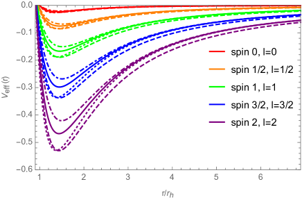
Figure 1: The effective potential for particles with spin.

In the near-horizon and infinite limit ($r_{\star}\to\mp\infty$), the effective potential takes the form

$$\begin{split}V_{\text{eff}}(r)&\overset{r_{\star}\to-\infty}{=}[(\omega-\omega_{+})-is\kappa_{+}]^{2}\\ &\overset{r_{\star}\to+\infty}{=}\omega(\omega+2is/r),\\ \end{split}$$ (160)

where $\omega_{+}$ is the critical value of angular frequency at the event horizon in Eq. (79). $\kappa_{+}$ is the surface gravities on the event horizon, as defined in Eq. (33). According to the RWZ equation in Eq. (123), there are two linearly independent solutions. In the near outer horizon limit $r\to r_{+}$ (i.e., $r_{\star}\to-\infty$), we have

$$\begin{split}\Psi^{s}&\overset{r_{\star}\to-\infty}{=}c_{1}e^{s\kappa_{+}r_{\star}}e^{i(\omega-\omega_{+})r_{\star}}+c_{2}e^{-s\kappa_{+}r_{\star}}e^{-i(\omega-\omega_{+})r_{\star}}\\ &\overset{r\to r_{+}}{=}c_{1}\Delta^{s/2}e^{i(\omega-\omega_{+})r_{\star}}+c_{2}\Delta^{-s/2}e^{-i(\omega-\omega_{+})r_{\star}},\\ \end{split}$$ (161)

where in the second row, we have used tortoise coordinate in Eq. (85) with the near event horizon behavior as

$$r_{\star}\overset{r\to r_{+}}{=}r_{+}+\frac{1}{2\kappa_{+}}\ln\frac{r-r_{+}}{r_{+}-r_{-}}.$$ (162)

The mode associated with the coefficients $c_{1,2}$ corresponds to the outgoing and ingoing waves in the near horizons, respectively. In the infinite large distance limit $r\to\infty$ (or $r_{\star}\to-\infty$), the radial wave function $\Psi_{s}$ has the asymptotic behavior

$$\begin{split}\Psi^{s}&\overset{r_{\star}\to+\infty}{=}r_{\star}e^{-i\omega r_{\star}}\big{[}c_{3}U\left(-s+1,2,2i\omega r_{\star}\right)\\ &+c_{4}\,{}_{1}F_{1}\left(-s+1;2;2i\omega r_{\star}\right)\big{]},\end{split}$$ (163)

where ${}_{1}F_{1}(a;b;z)$ is the Kummer confluent hypergeometric function and $U(a,b,z)$ is the confluent hypergeometric function. In the second row, we have used the tortoise coordinate in Eq. (85) with the lager distance asymptotic behavior as

$$r_{\star}\overset{r\to+\infty}{=}r+2M\ln\frac{r}{r_{+}-r_{-}}.$$ (164)

where the first term is a linearly increasing radial coordinate $r$, while the second term is a logarithmic increasing term. In this case, the asymptotic behavior of the radial wave function becomes

$$\Psi^{s}=\overset{r\to+\infty}{=}d_{1}r^{-s}e^{i\omega r}+d_{2}r^{s}e^{-i\omega r},$$ (165)

where $d_{1}$ is a constant involving both $c_{3}$ and $c_{4}$, and $d_{2}$ is one proportional to $c_{4}$. The mode associated with the coefficients $d_{1,2}$ corresponds to the outgoing and ingoing waves at large distances, respectively. According to Eq. (155), we have

$$\begin{split}R^{s}&\overset{r\to r_{+}}{=}\Delta^{-s/2}\Psi^{s},\quad R^{s}\overset{r\to\infty}{=}r^{-1-s}\Psi^{s}.\\ \end{split}$$ (166)

The near-horizon behavior of the radial wave function can be reexpressed as

$$\begin{split}R^{s}&=c_{1}\Delta^{-s}e^{-i(\omega-\omega_{+})r}(r-r_{+})^{-i\nu_{+}}\\ &+c_{2}e^{i(\omega-\omega_{+})r}(r-r_{+})^{i\nu_{+}}\\ &\overset{r\to r_{+}}{=}c_{1}(r-r_{+})^{-s-i\nu_{+}}+c_{2}(r-r_{+})^{i\nu_{+}}.\end{split}$$ (167)

It has a divergent phase for $r=r_{+}$. The exponential index $\nu_{+}$ is defined in Eq. (78), where $T_{+}$ is the Hawking temperature and $\kappa_{+}$ is the surface gravity. Therefore, the near-event horizon behavior and the large-distance behavior of the radial wave function $R$ are, respectively,

$$\begin{split}R^{s}&\overset{r\to r_{+}}{=}X_{\text{out}}^{s}e^{i(\omega-\omega_{+})r_{\star}}+X_{\text{in}}^{s}\Delta^{-s}e^{-i(\omega-\omega_{+})r_{\star}},\\ R^{s}&\overset{r\to+\infty}{=}Y_{\text{out}}^{s}r^{-2s-1}e^{i\omega r}+Y_{\text{in}}^{s}r^{-1}e^{-i\omega r},\\ \end{split}$$ (168)

where $X_{\text{out}}^{s}\propto c_{1},X_{\text{in}}^{s}\propto c_{2}$ corresponds to the amplitudes of outgoing and ingoing (transition) waves at the near event horizon region, and $Y_{\text{out}}^{s}\propto d_{1},Y_{\text{in}}^{s}\propto d_{2}$ corresponds to the amplitudes of outgoing (reflection) and ingoing waves at spatial infinity, respectively. This is a generalization of the scalar case in Eq. (130).

The near-horizon behavior of the radial wave function at $r=r_{+}$ is $R\sim e^{i(\omega-\omega_{+})r_{\star}}$ and $R\sim e^{-i(\omega-\omega_{+})r_{\star}}\Delta^{-s}$ (ingoing). $r_{\star}(r_{+})\to-\infty$ is the tortoise coordinate. The factor $\Delta^{-s}$ is not a physical singularity, but due to the choice of the generalized Kinnersley tetrad in Eq. (135), which is singular at horizons. Thus, the asymptotic solution to the radial wave function $R$ at spatial infinity $r=\infty$ is $R\sim r^{-1-2s}e^{i\omega r}$ (outgoing waves) and $R\sim r^{-1}e^{-i\omega r}$ (ingoing waves), respectively. They correspond to

$$\begin{split}&\phi,\chi_{1},\varphi_{2},\psi_{3},\Psi_{4}\sim r^{-1}e^{i\omega r},\quad\chi_{0}\sim r^{-2}e^{i\omega r},\quad\varphi_{0}\sim r^{-3}e^{i\omega r},\quad\psi_{0}\sim r^{-4}e^{i\omega r},\quad\Psi_{0}\sim r^{-5}e^{i\omega r},\quad(\text{outgoing}),\\ &\phi,\chi_{0},\varphi_{0},\psi_{0},\Psi_{0}\sim r^{-1}e^{-i\omega r},\quad\chi_{1}\sim r^{-2}e^{-i\omega r},\quad\varphi_{2}\sim r^{-3}e^{-i\omega r},\quad\psi_{3}\sim r^{-4}e^{-i\omega r},\quad\Psi_{4}\sim r^{-5}e^{-i\omega r},\quad(\text{ingoing}),\\ \end{split}$$ (169)

where we adopt the notations $\Phi^{s}=\{\phi,\chi,\varphi,\psi,\Psi\}$ to denote scalar, neutrino, Maxwell, Rarita-Schwinger, and gravitational fields, respectively. We identify $\{\phi,\chi_{1},\varphi_{2},\psi_{3},\Psi_{4}\}$ ($s\leq 0$) as the outgoing radiative part of the fields, and identify $\{\psi,\chi_{0},\varphi_{0},\psi_{0},\Psi_{0}\}$ as the ingoing radiative part of those fields, since they all decay as $1/r$. All other Newman-Penrose components of the fields decay more rapidly than $1/r$. Note that for a massless scalar field, both the outgoing and ingoing waves decay as $r^{-1}$. This is obvious by observing Eq. (130). In general, the complex tetrad components of gravitational waves at null infinity behave as

$$\begin{split}&\chi_{i=0,1}\sim r^{-2+i}e^{i\omega r},\quad\varphi_{i=0,1,2}\sim r^{-3+i}e^{i\omega r},\quad\psi_{i=0,1,2,3}\sim r^{-4+i}e^{i\omega r},\quad\Psi_{i=0,1,2,3,4}\sim r^{-5+i}e^{i\omega r}\quad(\text{outgoing}),\\ &\chi_{i=0,1}\sim r^{-1-i}e^{-i\omega r},\quad\varphi_{i=0,1,2}\sim r^{-1-i}e^{-i\omega r},\quad\psi_{i=0,1,2,3}\sim r^{-1-i}e^{-i\omega r},\quad\Psi_{i=0,1,2,3,4}\sim r^{-1-i}e^{-i\omega r}\quad(\text{ingoing}).\\ \end{split}$$ (170)

For massless scalar fields, outgoing and ingoing waves behave as $r^{-1}e^{\pm i\omega r}$. In summary, for an arbitrary spin-weighted particle, we have

$$\begin{split}&\Phi^{s}_{n=0,1,\ldots 2s}=Y^{s}_{\text{out}}r^{n-2s-1}e^{i\omega r_{\star}}\quad(\text{outgoing}),\\ &\Phi^{s}_{n=0,1,\ldots 2s}=Y^{s}_{\text{in}}r^{n-1}e^{-i\omega r_{\star}}\quad(\text{ingoing}),\\ \end{split}$$ (171)

where $Y^{s}_{\text{out}}$ and $Y^{s}_{\text{in}}$ are associated amplitudes. The ratio of powers $r^{|2s|}$ is due to the “peeling off” property [120].

V Low-energy dynamics of superradiance

V.1 Radial equations at low frequencies

We can also rewrite the radial wave function in Eq. (152) as

$$\begin{split}&\bigg{[}x(1+x)\frac{d^{2}}{dx^{2}}+(1+s)(1+2x)\frac{d}{dx}+\bigg{(}-\lambda+4is[(r_{+}-r_{-})x+r_{+}]\omega+\frac{[\omega((r_{+}-r_{-})x+r_{+})^{2}+a^{2}+n^{2}-2anC)-am]^{2}}{(r_{+}-r_{-})^{2}x(1+x)}\\ &-\frac{2is[(r_{+}-r_{-})x+r_{+}-M][\omega((r_{+}-r_{-})x+r_{+})^{2}+a^{2}+n^{2}-2anC)-am]}{(r_{+}-r_{-})^{2}x(1+x)}\bigg{)}\bigg{]}R_{s}=0,\\ \end{split}$$ (172)

where the primes are with respect to a variable $x$ as

$$x\equiv\frac{r-r_{+}}{r_{+}-r_{-}}.$$ (173)

Similarly, we can express the angular parameter $a$ as

$$a=\frac{(r_{+}-r_{-})\Omega_{+}}{4\pi T_{+}}=\frac{A\Omega_{+}}{4\pi},$$ (174)

where $\Omega_{+}$ is the angular velocity of the event horizon as defined in Eq. (36), $T_{+}$ is the Hawking temperature in Eq. (32), and $A_{+}$ is the area of the event horizon in Eq. (30). The equation becomes:

$$\begin{split}&x^{2}(1+x)^{2}R_{s}^{\prime\prime}+(1+s)x(1+x)(1+2x)R_{s}^{\prime}\\ &+\big{[}-x(1+x)\lambda+(\nu_{+}+k_{0}x^{2}+2r_{+}\omega x)^{2}\\ &+is[-(1+2x)\nu_{+}+k_{0}x^{2}(3+2x)+2r_{+}\omega x]\big{]}R_{s}=0,\\ \end{split}$$ (175)

where $\nu_{+}$ is defined in Eq. (78). $k_{0}$ is a dimensionless variable introduced in Eq. (73) with $k=\omega$, which can also be expressed in terms of physical observables as

$$k_{0}=\omega T_{\pm}A_{\pm},$$ (176)

where $A_{\pm}$ is the area of horizon defined in Eq.(30). In the approximation that the Compton wavelength of the particle is much larger than the gravitational size of the black hole, i.e., $M\omega\ll 1$ and the slowly rotating limit $a\omega\ll 1$, we have

$$\begin{split}&x^{2}(1+x)^{2}R_{s}^{\prime\prime}+(1+s)x(1+x)(1+2x)R_{s}^{\prime}\\ &+[-x(1+x)\lambda+\nu_{+}^{2}-is\nu_{+}(2x+1)\\ &+(2\nu_{+}+3is)k_{0}x^{2}+2isk_{0}x^{3}+k_{0}^{2}x^{4}]R_{s}=0,\\ \end{split}$$ (177)

with $k_{0}\ll 1$. The integral constant is defined through Eq. (54) as

$$\lambda=\bar{\lambda}-2a\bar{m}\omega+a^{2}\omega^{2}.$$ (178)

In the $a\omega\ll 1$, the angular eigenvalue becomes

$$\begin{split}\lambda&=\bar{\lambda}+a^{2}\omega^{2}-2am\omega=(l-s)(l+s+1),\end{split}$$ (179)

where $l-s$ is a non-negative integer.

V.1.1 Near-region solution

In the near region limit, i.e., $k_{0}x\ll 1$, the equation becomes

$$\begin{split}&x^{2}(1+x)^{2}R_{s}^{\prime\prime}+(1+s)x(1+x)(1+2x)R_{s}^{\prime}\\ &+[-\bar{\lambda}x(1+x)+\nu_{+}^{2}-is\nu_{+}(2x+1)]R_{s}=0.\\ \end{split}$$ (180)

In the $a\omega\ll 1$, the eigenvalue of angular equation is given by Eq. (148), i.e., $\bar{\lambda}=(l-s)(l+s+1)-\bar{s}^{2}\geq 0$. $l-s$ is a non-negative integer. The most general solution to the equation is a spin-weighted radial wave function in the form of

$$\begin{split}R^{s}&=x^{\alpha-s/2}(1+x)^{\beta-s/2}[c_{1}\,{}_{2}F_{1}(a,b;c;-x)\\ &+c_{2}x^{1-c}\,_{2}F_{1}(a-c+1,b-c+1;2-c;-x)],\end{split}$$ (181)

where the coefficients are

$$\begin{split}&\alpha=-\frac{s}{2}-i\nu_{+},\quad\beta=-\frac{s}{2}+i\nu_{+},\\ &a=-l-s,\quad b=l-s+1,\quad c=1-s-2i\nu_{+}.\\ \end{split}$$ (182)

The mode associated with $c_{2}$ corresponds to the ingoing wave for super-radiance, i.e., $\nu_{+}<0$. In the near-horizon limit, we have

$$R^{s}\overset{x\to 0}{=}c_{1}x^{-s-i\nu_{+}}+c_{2}x^{i\nu_{+}}.$$ (183)

It recovers the near-horizon behavior in Eq. (167) in the radial coordinate. The causality entails that we have to choose the ingoing boundary condition so that at the horizon, the wave is always ingoing, i.e., there is no outgoing mode at the horizon. By imposing the ingoing boundary conditions on the horizon, we obtain

$$\begin{split}R_{s}&=c_{1}x^{-s-i\nu_{+}}(1+x)^{-s+i\nu_{+}}\\ &\,{}_{2}F_{1}(-l-s,l-s+1;1-s-2i\nu_{+};-x).\\ \end{split}$$ (184)

In the infinity limit of $x$, the radial wave function behaves as

$$\begin{split}R_{s}&\overset{x\to\infty}{=}c_{1}\bigg{(}x^{l-s}\frac{\Gamma(2l+1)\Gamma(-s-2i\nu_{+}+1)}{\Gamma(l-2i\nu_{+}+1)\Gamma(l-s+1)}\\ &+x^{-l-s-1}\frac{\Gamma(-2l-1)\Gamma(-s-2i\nu_{+}+1)}{\Gamma(-l-2i\nu_{+})\Gamma(-l-s)}\bigg{)}.\\ \end{split}$$ (185)

V.1.2 Far region solution

At a large distance for $x\gg 1+|\nu|$, the first three terms in the second row of Eq. (177) can be dropped, and the differential equation is approximated by

$$\begin{split}&R_{s}^{\prime\prime}(x)+\frac{2(1+s)}{x}R_{s}^{\prime}(x)\\ &+\bigg{(}-\frac{\bar{\lambda}}{x^{2}}+\frac{(2\nu_{+}+3is)k_{0}}{x^{2}}+\frac{2isk_{0}}{x}+k_{0}^{2}\bigg{)}R_{s}(x)=0.\\ \end{split}$$ (186)

Given the eigenvalue in Eq. (148), in the low-frequency limit, i.e., $k_{0}\ll 1$, the solution simplifies as

$$\begin{split}R_{s}(x)&=e^{-ikx}x^{l-s}[c_{3}U(l-s+1,2l+2,2ikx)\\ &+c_{4}L_{-l+s-1}^{2l+1}(2ikx)],\\ \end{split}$$ (187)

where $U(a,b,c)$ is the confluent hypergeometric function, and $L_{n}(x)$ is the Laguerrel polynomial. In the far region, the equation can also be rewritten as

$$\begin{split}&\bigg{(}\frac{d^{2}}{dx^{2}}-[\bar{\lambda}+s(s+1)\\ &-2k_{0}\nu_{+}-ik_{0}s(3+2x)-k_{0}^{2}x^{2}]\bigg{)}\Psi_{s}=0,\end{split}$$ (188)

where $\Psi_{s}=x^{1+s}R_{s}$. The exact solution in the far region is

$$R_{s}=x^{-s-1}[c_{5}W_{s,l+1/2}(2ik_{0}x)+c_{6}M_{s,l+1/2}(2ik_{0}x)].\quad$$ (189)

In the near-horizon region, the solution is behaviors as

$$R_{s}(x)\overset{x\ll 1}{=}d_{1}^{s}x^{l-s}+d_{2}^{s}x^{-1-l-s},$$ (190)

where

$$\begin{split}&d_{1}^{s}=\frac{c_{3}\Gamma(-2l-1)}{\Gamma(-l-s)}+\frac{c_{4}\Gamma(l+s+1)}{\Gamma(2l+2)\Gamma(s-l)},\quad d_{2}^{s}=-\frac{ic_{3}4^{-l}e^{-i\pi l}lk_{0}^{-2l-1}\Gamma(2l)}{\Gamma(l-s+1)}.\\ \end{split}$$ (191)

On the other hand, by matching to Eq. (185), the coefficients $d_{1,2}$ are determined as

$$\begin{split}&d_{1}^{s}=c_{1}\frac{\Gamma(2l+1)\Gamma(-s-2i\nu_{+}+1)}{\Gamma(l-2i\nu_{+}+1)\Gamma(l-s+1)},\quad d_{2}^{s}=c_{1}\frac{\Gamma(-2l-1)\Gamma(-s-2i\nu_{+}+1)}{\Gamma(-l-2i\nu_{+})\Gamma(-l-s)}.\end{split}$$ (192)

From which, we can determine $c_{3,4}$ as

$$\begin{split}c_{3}^{s}&=\frac{ic_{1}4^{l}e^{i\pi l}k^{2l+1}\Gamma(-2l-1)\Gamma(l-s+1)\Gamma(-s-2i\nu_{+}+1)}{l\Gamma(2l)\Gamma(-l-2i\nu_{+})\Gamma(-l-s)},\\ c_{4}^{s}&=c_{1}\Gamma(-s-2i\nu_{+}+1)\bigg{(}\frac{\Gamma(2l+1)\Gamma(2l+2)\Gamma(s-l)}{\Gamma(l-2i\nu_{+}+1)\Gamma(l-s+1)\Gamma(l+s+1)}-\frac{i2^{2l+1}e^{i\pi l}(2l+1)k_{0}^{2l+1}\Gamma(-2l-1)^{2}\sin(\pi(l+s))}{\Gamma(-l-2i\nu_{+})\Gamma(-l-s)\sin(\pi(l-s))}\bigg{)}.\\ \end{split}\quad$$ (193)

In the infinite limit, we have

$$\begin{split}R_{s}&\overset{x\to\infty}{=}Y^{s}_{\text{in}}e^{-i\omega(r-r_{+})}r^{-1}+Y^{s}_{\text{out}}e^{i\omega(r-r_{+})}r^{-2s-1},\\ \end{split}$$ (194)

where the ingoing and outgoing wave amplitudes at infinity are

$$\begin{split}&Y^{s}_{\text{in}}=\frac{i^{1-l-s}}{(2k_{0})^{1+l+s}}(2k_{0})^{2s}\bigg{(}\frac{e^{il\pi}c_{4}}{\Gamma(-l+s)}-c_{3}e^{i\pi s}\bigg{)}\frac{k_{0}}{\omega},\quad Y^{s}_{\text{out}}=-\frac{i^{1-l-s}}{(2k_{0})^{1+l+s}}\frac{c_{4}\Gamma(l+s+1)}{\Gamma(l-s+1)\Gamma(s-l)}\bigg{(}\frac{k_{0}}{\omega}\bigg{)}^{2s+1}.\end{split}$$ (195)

The factor $k_{0}/\omega$ comes from the coordinate transformation, since according to Eq. (173) and (176), we have

$$x=\frac{\omega}{k_{0}}(r-r_{+}).$$ (196)

Thus, we obtain the reflection coefficient:

$$\begin{split}\frac{Y^{s}_{\text{out}}}{Y^{s}_{\text{in}}}&=-\frac{e^{-il\pi}}{(2\omega)^{2s}}\frac{\Gamma(l+s+1)}{\Gamma(l-s+1)+\pi[\cot[\pi(l-s)]-i](c_{3}^{s}/c_{4}^{s})},\\ \end{split}\quad$$ (197)

where the ratio of the constants is

$$\begin{split}&\frac{c_{3}^{(s)}}{c_{4}^{(s)}}=-\frac{\Gamma(l-s+1)}{\pi}\frac{\sin{(2\pi l)}}{\cos{(2\pi s)}-i\frac{e^{-il\pi}}{(2k_{0})^{2l+1}}\frac{\Gamma(l+1)\Gamma(2l+2)\Gamma(-l-s)^{2}\Gamma(-l-2i\nu_{+})}{\Gamma(-2l-1)\Gamma(-2l)\Gamma(l-s+1)^{2}\Gamma(l+1-2i\nu_{+})}}.\\ \end{split}$$ (198)

From this, we immediately obtain the radial wave function $R_{-s}$ by solving the radial equation with $s$ replaced by $-s$ to get the asymptotic form as

$$\begin{split}R^{-s}&=Z^{s}_{\text{in}}e^{-i\omega(r-r_{+})}r^{-1}+Z^{s}_{\text{out}}e^{i\omega(r-r_{+})}r^{2s-1},\end{split}$$ (199)

where the superscript index $s$ denotes its spin dependence with the relevant sign and

$$\begin{split}&Z^{s}_{\text{in}}\equiv Y^{-s}_{\text{in}}=(2k_{0})^{-2s}\bigg{(}\frac{e^{il\pi}d_{2}^{-s}}{\Gamma(-l-s)}-d_{1}^{-s}e^{-i\pi s}\bigg{)}\frac{k_{0}}{\omega},\quad Z^{s}_{\text{out}}\equiv Y^{-s}_{\text{out}}=-\frac{\Gamma(l-s+1)}{\Gamma(l+s+1)\Gamma(-s-l)}d_{2}^{-s}\bigg{(}\frac{k_{0}}{\omega}\bigg{)}^{-2s+1}.\end{split}\quad$$ (200)

V.2 low-energy dynamical observables

V.2.1 Amplification factor

The amplification factor is defined as

$${\mathrm{A}}^{s}\equiv{\mathrm{R}}^{s}-1=-\Gamma^{s},$$ (201)

where ${\mathrm{R}}^{s}\equiv|{\mathcal{R}}^{s}|^{2}$ is the reflection coefficient and $\Gamma^{s}\equiv|{\mathcal{T}}^{s}|^{2}$ is the transition coefficient. They stand for the reflection probability and transmission probability, respectively. The reflection coefficient ${\mathrm{R}}^{s}$ is defined as

$${\mathrm{R}}^{s}=\left|\frac{Y^{s}_{\text{out}}}{Y^{s}_{\text{in}}}\frac{Z^{s}_{\text{out}}}{Z^{s}_{\text{in}}}\right|=1-\Gamma^{s},$$ (202)

where $Y^{s}$ and $Z^{s}$ are given in Eqs. (195) and (200). Thus, we obtain $\Gamma^{s}=1-{\mathrm{R}}^{s}=-{\mathrm{A}}^{s}$. It is equivalent to the absorption probability, also in terms of the graybody factor . Note that at low frequencies, we can make perturbative expansions as

$$\begin{split}\frac{Y^{s}_{\text{out}}}{Y^{s}_{\text{in}}}\frac{Z^{s}_{\text{out}}}{Z^{s}_{\text{in}}}&=e^{-2il\pi}\bigg{[}1-e^{i\pi(s-1/2)}\bigg{(}3+\frac{\sin{\pi(l-3s)}}{\sin{\pi(l+s)}}\bigg{)}\cos{\pi(l-s)}\frac{\Gamma(-2l-1)\Gamma(-2l)\Gamma(l-s+1)^{2}}{\Gamma(2l+1)\Gamma(2l+2)\Gamma(-l-s)^{2}}\\ &\times\frac{\Gamma(l+1-2i\nu_{+})}{\Gamma(-l-2i\nu_{+})}(2k_{0})^{2l+1}+O(k_{0}^{4l+2})\bigg{]},\\ \end{split}\qquad$$ (203)

where we have imposed the constraint that $2s\in{\mathcal{Z}}$. Thus, $\sin[\pi(l+s)]=\sin{[\pi(l-s)]}$ etc., and $l-s>0$.

V.2.2 Gray body factor

The absorption probability, or gray body factor, is

$$\begin{split}\Gamma^{s}&=\text{Re}\bigg{[}4e^{-i\pi(l-s)}\cos{\pi(l-s)}\frac{\sin^{2}{[\pi(l+s)]}}{\sin^{2}(2\pi l)}\frac{\Gamma(l-s+1)^{2}\Gamma(l+s+1)^{2}}{\Gamma(2l+1)^{2}\Gamma(2l+2)^{2}}\frac{\Gamma(l+1-2i\nu_{+})}{\Gamma(-l-2i\nu_{+})}(2ik_{0})^{2l+1}\bigg{]}.\\ \end{split}$$ (204)

Only the real part in the bracket is relevant, since the reflection coefficient is a real number. Assuming that $2s,2l\in{\mathbb{Z}}$, and $l-s\in{\mathbb{Z}}^{+}$, then we can write the absorption probability as

$$\begin{split}\Gamma^{s}&=\text{Re}\bigg{[}\bigg{(}\frac{(l-s)!(l+s)!}{(2l)!(2l+1)!}\bigg{)}^{2}\frac{\Gamma(l+1-2i\nu_{+})}{\Gamma(-l-2i\nu_{+})}(2ik_{0})^{2l+1}\bigg{]},\\ &\\ \end{split}\qquad$$ (205)

where the real index $\nu_{+}$ is defined in Eq. (78). We can express it in terms of observables as

$$\begin{split}\nu_{+}&=\frac{\omega-m\Omega_{+}}{2\kappa_{+}}=\frac{\omega-m\Omega_{+}}{4\pi T_{+}},\\ \end{split}$$ (206)

where $\kappa_{+}$ is the surface gravity on the event horizon in Eq. (33) and $T_{+}$ is the Hawking temperature in Eq. (32). $\Omega_{+}$ is the angular velocity on the event horizon defined through Eq. (79). When $a=n=0$, $\nu_{+}=2M\omega$ it recovers the Schwarzschild case. By replacing the dimensionless variable $k_{0}$ in Eq. (176), we obtain the absorption probability as low frequency as

$$\begin{split}\Gamma^{s}_{lm}&=\bigg{(}2^{l}l!\frac{(l-s)!(l+s)!}{(2l)!(2l+1)!}\bigg{)}^{2}\prod_{n=1}^{l}\bigg{[}1+\bigg{(}\frac{1}{n}\frac{\omega-m\Omega_{+}}{2\pi T_{+}}\bigg{)}^{2}\bigg{]}\frac{\omega-m\Omega_{+}}{\pi T_{+}}(A_{+}T_{+}\omega)^{2l+1},\quad 2l\in\text{even},\\ &=\bigg{(}2^{l}l!\frac{(l-s)!(l+s)!}{(2l)!(2l+1)!}\bigg{)}^{2}\prod_{n=1}^{l+1/2}\bigg{[}1+\bigg{(}\frac{1}{n-1/2}\frac{\omega-m\Omega_{+}}{2\pi T_{+}}\bigg{)}^{2}\bigg{]}\frac{2}{\pi}(A_{+}T_{+}\omega)^{2l+1},\quad 2l\in\text{odd},\\ \end{split}$$ (207)

where we have to take into account that $2l$ can be an even or odd integer, which corresponds to $l$ being an integer or half integer integer, separately. We have added the subscript $(l,m)$ to indicate that $\Gamma^{s}$ depends on the angular orbital and magnetic quantum number. On the right side of the formula, we have replaced the dimensionless variable $k_{0}$ by observables by substituting Eq. (176). The common factor in front of the absorption probability formula for both bosons and fermions is

$$2^{l}l!\frac{(l-s)!(l+s)!}{(2l)!(2l+1)!}\overset{l=s}{=}\frac{2^{s}s!}{(2s+1)!}.$$ (208)

The maximal value is achieved at $l=s$ mode, which is the dominant contribution to the absorption probability. Since $l\geq s$, it decays rapidly when $l\gg s$. The first row corresponds to the bosons, and the second line corresponds to fermions. It is clear the absorption probability for bosons is negative, which means the bosonic fields (particles or waves) are amplified rather than absorbed at low frequency. However, the absorption probability for femions is always positive, which implies there is no superradiance for fermions at low frequencies. We can also reexpress the gray body factor in a form

$$\begin{split}\Gamma^{s}_{lm}&=\bigg{(}2^{l}\frac{(l-s)!(l+s)!}{(2l)!(2l+1)!}\bigg{)}^{2}\left|\Gamma\left(l+1+\frac{i(\omega-m\Omega_{+})}{2\pi T_{+}}\right)\right|^{2}\frac{2}{\pi}(A_{+}T_{+}\omega)^{2l+1}\sinh\bigg{(}\frac{\omega-m\Omega_{+}}{2T_{+}}\bigg{)},\quad 2l\in\text{even},\\ &=\bigg{(}2^{l}\frac{(l-s)!(l+s)!}{(2l)!(2l+1)!}\bigg{)}^{2}\left|\Gamma\left(l+1+\frac{i(\omega-m\Omega_{+})}{2\pi T_{+}}\right)\right|^{2}\frac{2}{\pi}(A_{+}T_{+}\omega)^{2l+1}\cosh\bigg{(}\frac{\omega-m\Omega_{+}}{2T_{+}}\bigg{)},\quad 2l\in\text{odd}.\\ \end{split}$$ (209)

The $\sinh{x}$ and $\cosh{x}$ are odd and even functions, respectively. For bosons, $\Gamma^{s}_{lm}$ reverses the sign when $\omega$ crosses the resonance point $m\Omega_{+}$. For fermions, $\Gamma^{s}_{lm}$ is always positive. Thus, there is no superradiance for fermions. To be concrete, let’s consider the scalar field ($s=0$), neutrino field ($s=1/2$), electromagnetic wave ($s=1$), Rarita-Schwinger field (vector spinor) ($s=3/2$), and gravitational wave ($s=2$), separately. The low-frequency absorption probability for these fields is

$$\begin{split}\Gamma^{0}_{0m}&=\frac{A_{+}}{\pi}(\omega-m\Omega_{+})\omega,\\ \Gamma^{1/2}_{1/2m}&=\bigg{[}(M^{2}-a^{2}+n^{2})+\bigg{(}\frac{A_{+}}{2\pi}\omega-2am\bigg{)}^{2}\bigg{]}\omega^{2},\\ \Gamma^{1}_{1m}&=\frac{4A_{+}}{9\pi}\bigg{[}M^{2}+n^{2}-a^{2}+\bigg{(}\frac{A_{+}}{4\pi}\omega-am\bigg{)}^{2}\bigg{]}(\omega-m\Omega_{+})\omega^{3},\\ \Gamma^{3/2}_{3/2m}&=\frac{1}{8}\bigg{[}M^{2}+n^{2}-a^{2}+\bigg{(}\frac{A_{+}\omega}{2\pi}-2am\bigg{)}^{2}\bigg{]}\bigg{[}M^{2}+n^{2}-a^{2}+\bigg{(}\frac{A_{+}\omega}{6\pi}-\frac{2am}{3}\bigg{)}^{2}\bigg{]}\omega^{4},\\ \Gamma^{2}_{2m}&=\frac{16}{225}\frac{A_{+}}{\pi}\bigg{[}M^{2}+n^{2}-a^{2}+\bigg{(}\frac{A_{+}\omega}{4\pi}-am\bigg{)}^{2}\bigg{]}\bigg{[}M^{2}+n^{2}-a^{2}+\bigg{(}\frac{A_{+}\omega}{8\pi}-\frac{1}{2}am\bigg{)}^{2}\bigg{]}(\omega-m\Omega_{+})\omega^{5},\\ \end{split}$$ (210)

where $A_{+}$ is the area of the outer horizon as defined in Eq. (30). It contributes to the BH entropy of the KTN black hole, according to Eq. (31). We have also used that

$$A_{+}\Omega_{+}=4\pi a,\quad A_{+}T_{+}=2\sqrt{M^{2}+n^{2}-a^{2}}.$$ (211)

By keeping the lowest order terms in $\omega$, except for the $\omega-m\Omega_{+}$ factor for bosons, which guarantees that the superradiant condition $\omega<a\omega_{+}$ satisfies, we obtain the absorption probability at ultra low frequency as

$$\begin{split}\Gamma^{0}_{0m}&=\frac{A_{+}}{\pi}(\omega-m\Omega_{+})\omega,\\ \Gamma^{1/2}_{1/2m}&\overset{\omega\ll 1}{=}[M^{2}+n^{2}+(4m^{2}-1)a^{2}]\omega^{2},\\ \Gamma^{1}_{1m}&\overset{\omega\ll 1}{=}\frac{4}{9}[M^{2}+n^{2}+(m^{2}-1)a^{2}]\omega^{2}\Gamma^{0}_{0m},\\ \Gamma^{3/2}_{3/2m}&\overset{\omega\ll 1}{=}\frac{1}{8}[M^{2}+n^{2}+(4m^{2}/9-1)a^{2}]\omega^{2}\Gamma^{1/2}_{1/2m},\\ \Gamma^{2}_{2m},&\overset{\omega\ll 1}{=}\frac{4}{25}[M^{2}+n^{2}+(m^{2}/4-1)a^{2}]\omega^{2}\Gamma^{1}_{1m}.\\ \end{split}$$ (212)

To compare the relative amplitudes of the absorption probability, we have expressed that of higher spin fields with that of lower spin fields. The absorption probability of the Rarita-Schwinger wave (spin-$3/2$) is expressed in terms of that of the neutrino wave (spin-$1/2$). The absorption probability of the gravitational wave (spin-$2$) is expressed in terms of that of an electromagnetic wave (spin-$1$), which is expressed in terms of that of a scalar wave (spin-$0$). We also obtain a new result for the massless Rarita-Schwinger field. In contrast to the case of the bosons, i.e., integer spin perturbation fields, the lack of the factor $(\omega-m\Omega_{+})$ in the gray body factor indicates that fermions, i.e., half-integer spin perturbation fields, do not exhibit superradiance.

V.2.3 Absorption cross section

With the analytic absorption probabilities at low frequencies for the various angular modes for spin-$s$ weighted massless boson and fermion fields, including scalar, neutrino, electromagnetic, Rarita-Schwinger, and gravitational waves in the KTN black hole, we can obtain the low-frequency, i.e., $M\omega\ll 1$ absorption cross section for a massless particle of spin $s$ averaged over all orientations of the spacetime 

$$\sigma^{s}=\sum_{l=s}^{\infty}\sigma^{s}_{l},$$ (214)

where the $l$-mode of the partial wave cross section of the spin-$s$ particle is

$$\sigma^{s}_{l}=\sum_{m=-l}^{l}\sigma^{s}_{lm}=\frac{\pi}{\omega^{2}}\sum_{m=-l}^{l}\Gamma^{s}_{lm}.$$ (215)

The dominant $l=s$ mode contributes to the absorption cross section as

$$\begin{split}\sigma^{0}_{0}(\omega)&=A_{+},\\ \sigma^{1/2}_{1/2}(\omega)&=2\pi(M^{2}+n^{2})+\frac{A_{+}^{2}}{2\pi}\omega^{2},\\ \sigma^{1}_{1}(\omega)&=\frac{4}{3}A_{+}[(M^{2}+n^{2}+a^{2})+\frac{A_{+}^{2}}{16\pi^{2}}\omega^{2}]\omega^{2},\\ \sigma^{3/2}_{3/2}(\omega)&=\frac{\pi}{18}\bigg{(}(M^{2}+n^{2})[9(M^{2}+n^{2})+32a^{2}]+\frac{5A_{+}^{2}}{2\pi^{2}}(M^{2}+n^{2}+2a^{2})\omega^{2}+\frac{A_{+}^{4}}{16\pi^{4}}\omega^{4}\bigg{)}\omega^{2},\\ \sigma^{2}_{2}(\omega)&=\frac{8}{45}A_{+}\bigg{(}[2(M^{2}+n^{2})^{2}+11(M^{2}+n^{2})a^{2}+4a^{4}]+\frac{5A_{+}^{2}}{32\pi^{2}}(M^{2}+n^{2}+3a^{2})\omega^{2}+\frac{A_{+}^{4}}{512\pi^{4}}\omega^{4}\bigg{)}\omega^{4}.\\ \end{split}$$ (216)

It’s worth noticing that at low frequency, the absorption cross section for the bosons is proportional to the area of the black hole $A_{+}$ in Eq. (217). It can be expressed more explicitly as

$$A_{+}=8\pi[M^{2}+n^{2}-anC+M\sqrt{M^{2}-a^{2}+n^{2}}].$$ (217)

It’s clear that the cross section depends not only on the NUT parameter but also on the MR parameter $C$ which describes the position of the defect along the polar axis. In the Schwarzschild limit, i.e., $a=n=0$, the dominant absorption cross section for $s=l=0$ reduces to the correct result for Schwarzschild black holes at low frequency as

$$\sigma^{0}_{0}=4\pi(2M)^{2}.$$ (218)

The cross sections at low frequencies $M\omega\ll 1$ are smaller than those at high frequencies $M\omega\gg 1$.  While for fermions, the absorption cross section is independent of the horizon area or entropy of the black hole. As frequencies go to zero, the absorption cross section for both electromagnetic waves and gravitational waves is zero, but that for massless scalar particles and neutrino particles remains at finite values. The cross sections go to zero as the frequency goes to the second power for photons as well as Rarita-Schwinger fermions, and to the fourth power for gravitons.

V.2.4 Emission rate of Hawking radiation

By combining the low-frequency absorption probability ${\mathrm{A}}^{s}=-\Gamma^{s}$ with the thermal factor $n_{s}(\omega,\omega_{+},T_{+})$ for a black hole with finite temperature, we can obtain the expected particle number (of the spin-$s$ species) with

$$\langle N^{s}_{lm}\rangle=\Gamma^{s}_{lm}n_{s},$$ (220)

where $n_{s}$ is the thermal statistical distribution of the spin-$s$ particle, which can be expressed in a unified form as

$$n_{s}=\frac{1}{e^{(\omega-\omega_{+})/T_{+}}-(-1)^{2s}}.$$ (221)

$T_{+}$ is the Hawking temperature in Eq. (32), and $\omega_{+}$ is the critical angular frequency at the event horizon in Eq. (79), which is related to the horizon angular velocity $\Omega_{+}$ and horizon electrostatic potential $\Phi_{+}$. In the low-frequency limi $\omega\ll 1$,

$$\begin{split}&n_{b}(\omega)=\frac{1}{e^{(\omega-\omega_{+})/T_{+}}-1}\overset{\omega\ll 1}{\approx}\frac{T_{+}}{\omega}-\frac{1}{2}+O(\omega)\ \\ &n_{f}(\omega)=\frac{1}{e^{(\omega-\omega_{+})/T_{+}}+1}\overset{\omega\ll 1}{\approx}\frac{1}{2}+O(\omega).\\ \end{split}$$ (222)

The minus and plus signs in the statical distribution for bosons ($b$) and fermions ($f$) are used, separately. For massive particles ($\omega\sim m\gg 1$), the statistical distribution is the Boltzmann one. The averaged emission rate per frequency interval $d\omega$ is related to the expected particle numbers through

$$\frac{dN^{s}_{lm}}{dt}=\left\langle N^{s}_{lm}\right\rangle\frac{d\omega}{2\pi}.$$ (223)

where $2\pi$ is a phase space factor. The emission rate is

$$\frac{dN^{s}_{lm}}{dtd\omega}=\frac{1}{2\pi}\left\langle N^{s}_{lm}\right\rangle=\frac{\Gamma^{s}_{lm}}{2\pi}n_{s},$$ (224)

where $\Gamma^{s}_{lm}$ is the gray body factor, and at low frequencies it is given in Eq. (207). For slow rotating (i.e., $a\ll 1$) or non-rotating black hole (i.e.,$a=0$), $\Omega_{+}\approx 0$, $A_{+}\Omega_{+}\approx 0$ and $A_{+}T_{+}\approx 2\sqrt{M^{2}+n^{2}}$, the Hawking temperature is $T_{+}=[4\pi(M+\sqrt{M^{2}+n^{2}})]^{-1}\ll 1$. Thus, the emission rate at low frequencies for both bosons and fermions is given by

$$\frac{dN^{s}_{lm}}{dtd\omega}=\frac{1}{2\pi^{2}}\bigg{(}2^{l}l!\frac{(l-s)!(l+s)!}{(2l)!(2l+1)!}\bigg{)}^{2}(2\sqrt{M^{2}+n^{2}}\omega)^{2l+1},$$

(225)

where we have approximated as below

$$\begin{split}&\prod_{n=1}^{l}\bigg{[}1+\bigg{(}\frac{1}{n}\frac{\omega}{2\pi T_{+}}\bigg{)}^{2}\bigg{]}\overset{\omega\ll 1}{\approx}1+O(\omega^{2}),\\ &\prod_{n=1}^{l+1/2}\bigg{[}1+\bigg{(}\frac{1}{n-1/2}\frac{\omega}{2\pi T_{+}}\bigg{)}^{2}\bigg{]}\overset{\omega\ll 1}{\approx}1+O(\omega^{2}).\\ \end{split}$$ (226)

This means at low frequencies, the emission rate goes as $\omega^{2l+1}$, thus the power $dN^{s}_{lm}/dt$ goes as $\omega^{2l+2}$. Consequently, the lower spin weighted particle (thus lower $l$ allowed since $l\geq s$) was emitted faster from a non-rotating black hole, thus dominating the low-frequency power drain from the black hole.

V.2.5 Power spectrum

The scattering of spin-$s$ particles will carry off energy $\epsilon=\hbar\omega$ and angular momentum $j=m$ about the axis of the black hole. According to the averaged emission rate, the mass and angular momentum of the black hole decrease at the rate given by the total energy and torque emitted as

$$\frac{d}{dt}\begin{pmatrix}M\\ J\\ \end{pmatrix}=-\sum_{l,m}\int\frac{dN^{s}_{lm}}{dt}\begin{pmatrix}\omega\\ m\\ \end{pmatrix},$$ (227)

where $l,m$ are the angular momentum and its azimuthal magnetic component, and $\omega$ is the energy of the massless particle. For the Hawking radiation of rotating spacetime, the emission rates of energy and angular momentum are 

$$\begin{split}\frac{d}{dt}\begin{pmatrix}M\\ J\\ \end{pmatrix}&=-\frac{1}{2\pi}\sum_{l,m}\int_{0}^{\infty}d\omega\Gamma^{s}_{lm}n_{s}\begin{pmatrix}\omega\\ m\\ \end{pmatrix},\end{split}$$ (228)

where $\Gamma^{s}$ is the emission rate in Eq. (225). It is related to the amplification factor ${\mathrm{A}}^{s}$ and reflection coefficient ${\mathrm{R}}^{s}$ at the infinite boundary through Eq. (201). It can be obtained by solving the radial Teukolsky equation. $\omega_{+}=m\Omega_{+}$ is the critical angular frequency in Eq. (79). $\Omega_{+}$ is the angular velocity on the event horizon. $T_{+}$ is the Hawking temperature in Eq. (32).

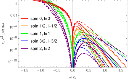
Figure 2: Energy power spectrum for particles with spin

In the extreme limit, the Hawking temperature $T_{+}$ vanishes, and Hawking radiation becomes purely superradiant, i.e., ${\mathrm{A}}^{s}>0$, that is, when $\omega<\omega_{+}$ and $T_{+}\to 0$. In this case, the emission rates are

$$\begin{split}\frac{d}{dt}\begin{pmatrix}M\\ J\\ \end{pmatrix}&=(-1)^{2s}\frac{1}{2\pi}\sum_{l,m}\int_{0}^{\infty}d\omega({\mathrm{R}}^{s}-1)\begin{pmatrix}\omega\\ m\\ \end{pmatrix}.\end{split}$$ (229)

There is a minus sign or a plus sign corresponding to the boson and fermion cases, separately. This indicates that the superradiant scattering of bosons leads to a decrease in the total mass and angular momentum of the KTN spacetime. Once we obtain the absorption probability (or the graybody factor) $\Gamma^{s}$, we can calculate the angular dependent power spectrum of the Hawking radiation for each massless spin-$s$ particle as

$$\frac{d^{2}E^{s}_{lm}}{dtd\Omega}=\frac{1}{2\pi}\Gamma^{s}_{lm}n_{s}|S^{s}_{lm}(c,\theta,\phi)|^{2}\omega d\omega,$$ (230)

where $d\Omega=d\phi d\cos\theta$ is the infinitesimal solid angle, $\omega_{+}=m\Omega_{+}$ is the critical angular frequency, $\Omega_{+}$ is the angular velocity at the horizon. $\Gamma^{s}_{lm}$ is the graybody factor, which is identical to the absorption probability of the incoming wave of the corresponding modes carrying angular orbital and magnetic quantum numbers. $S^{s}_{lm}$ is a spin-weighted spheroidal function. By integrating over the angular variables $(\theta,\phi)$, we obtain the angle-averaged energy power spectrum as

$$\frac{d^{2}E^{s}_{lm}}{dtd\omega}=\frac{1}{2\pi}\Gamma^{s}_{lm}n_{s}\omega.$$ (231)

At low frequencies, the power spectrum behaves as $\propto\omega^{2l+2}$. The energy power spectrum for massless scalar, neutrino, photon, Rarita-Schwinger field, and gravitons is shown in Fig. 2. We have chosen input parameters $M=1$, $n=0.5$, and $a=0.9$ (rapidly rotating), and set $m=0$ so that $d^{2}J/dtd\omega=0$. As has been discussed before, the MR parameter becomes irrelevant in the far region. The effect of $C$ is only incorporated through the definition of the Hawking temperature $T_{+}$ in Eq. (32), as well as the angular velocity in Eq. (36).

From bottom to top, it corresponds to the gravitational wave (purple), the Rarita-Schwinger wave (blue), the electromagnetic wave (green), the neutrino wave (orange), and the scalar wave (red), respectively. The dashed line corresponds to reference ones in the Kerr black hole, separately. In order to facilitate comparison, in the same figure, we have also plotted the energy power spectrum with different MR parameters: $C=0$ (solid lines), $C=+1$ (dotted lines), and $C=-1$ (dot-dashed lines), separately.

The figure shows that the energy power spectrum with the $C=-1$ case is larger than that with the $C=0$ and $C=+1$ cases. For three cases, the energy power spectrum for each massless spin-$s$ wave in the KTN spacetime is enhanced than that in the Kerr black hole.

In particular, they have different behaviors for $\omega>0$ (co-rotating) and $\omega<0$ (counter-rotating) regions. It is clear that the superradiance condition is always fulfilled in the counter-rotating region. Only scalar, electromagnetic, and gravitational waves are amplified.

The figure also verifies that there is no superradiance for fermions, i.e., half-integer spin perturbation fields do not exhibit superradiance. Intuitively, the superraidnce means boson fields in a rotating spacetime will gain extra energy, given that the fields are counter-rotating with respect to the rotation direction of the spacetime.

In the case that $S^{s}_{lm}(c,\theta,\phi)$ are frequency independent, i.e., $c=0$, the spin-weighted spheroidal harmonics $S^{s}_{lm}$ reduce to spin-weighted spherical harmonics $Y^{s}_{lm}$. By integrating over the angular variable $\phi$, we obtain the angular spectrum as

$$\frac{d^{3}E^{s}_{lm}}{dtd\cos\theta d\omega}=\frac{1}{2\pi}\Gamma_{lm}^{s}n_{s}I^{s}_{lm}(\cos\theta)\omega,$$ (232)

where $\theta\in[0,\pi]$ is the polar angle, and $\theta=0,\pi$ stands for forward and backward scattering, respectively. $s=0,1/2,1,3/2,2$, $l=0,1/2,3/2,1,2$, and $m=-l,\ldots,l$. $I^{s}_{lm}(\cos\theta)$ are polar angle distribution functions, after integrating over azimuthal angle as

$$I^{s}_{lm}(\cos\theta)=\int_{0}^{2\pi}d\phi|Y^{s}_{lm}(\cos\theta,\phi)|^{2}.$$ (233)

It stands for angular (spin, orbital, and azimuthal) dependent probability of wave function with quantum numbers $(s,l,m)$ for $s=0,1/2,1,3/2,2$, $l=0,1/2,3/2,1,2$, and $m=-l,\ldots,l$. With the explicit form of the spin-weighted spherical harmonics, as listed in the Appendix I.2.3, we can exactly integrate out the integral $I^{s}_{lm}$. For scalar wave ($l=s=0$), $Y^{s}_{0m}$ is ordinary scalar spherical harmonics, we have

$$I^{0}_{00}=\frac{1}{2}.$$ (234)

For neutrino wave ($l=s=1/2$), $Y^{s}_{lm}$ is spinor-valued spherical harmonics, we have

$$\begin{split}&I^{\pm 1/2}_{1/2,\mp 1/2}=\cos^{2}\frac{\theta}{2},\quad I^{\pm 1/2}_{1/2,\pm 1/2}=\sin^{2}\frac{\theta}{2}.\end{split}$$ (235)

For electromagnetic wave ($l=s=1$), $Y^{s}_{lm}$ is vector spherical harmonics, we have

$$\begin{split}&I^{-1}_{1,-1}=I^{1}_{1,1}=\frac{3}{2}\sin^{4}\frac{\theta}{2},\quad I^{-1}_{1,1}=I^{1}_{1,-1}=\frac{3}{2}\cos^{4}\frac{\theta}{2},\\ &I^{0}_{1,0}=\frac{3}{2}\cos^{2}\theta,\quad I^{-1}_{1,0}=I^{0}_{1,-1}=I^{0}_{1,1}=I^{1}_{1,0}=\frac{3}{4}\sin^{2}\theta.\\ \end{split}$$ (236)

For Rarita-Schwinger field ($l=s=3/2$), $Y^{s}_{lm}$ is spinor-valued vector spherical harmonics, we have

$$\begin{split}I^{-3/2}_{3/2,-3/2}&=I^{3/2}_{3/2,3/2}=2\sin^{6}\frac{\theta}{2},\\ I^{-3/2}_{3/2,3/2}&=I^{3/2}_{3/2,-1/2}=2\cos^{6}\frac{\theta}{2};\\ I^{-3/2}_{3/2,-1/2}&=I^{3/2}_{3/2,1/2}=I^{1/2}_{3/2,3/2}=I^{-1/2}_{3/2,-3/2}\\ &=\frac{3}{2}\sin^{2}\frac{\theta}{2}\sin^{2}\theta,\\ I^{-3/2}_{3/2,1/2}&=I^{3/2}_{3/2,-1/2}=I^{3/2}_{3/2,-3/2}=I^{-1/2}_{3/2,3/2}=I^{1/2}_{3/2,-3/2}\\ &=\frac{3}{2}\cos^{2}\frac{\theta}{2}\sin^{2}\theta,\\ I^{-1/2}_{3/2,-1/2}&=I^{1/2}_{3/2,1/2}=\frac{1}{2}\sin^{2}\frac{\theta}{2}(3\cos\theta+1)^{2},\\ I^{-1/2}_{3/2,1/2}&=I^{1/2}_{3/2,-1/2}=\frac{1}{2}\cos^{2}\frac{\theta}{2}(3\cos\theta-1)^{2}.\\ \end{split}$$ (237)

For gravitational wave ($l=s=2$), $Y^{s}_{lm}$ is tensor spherical harmonics, we have

$$\begin{split}&I^{-2}_{2,-2}=I^{2}_{2,2}=\frac{5}{2}\sin^{8}\frac{\theta}{2},\\ &I^{-2}_{2,2}=I^{2}_{2,-2}=\frac{5}{2}\cos^{8}\frac{\theta}{2};\\ &I^{-2}_{2,-1}=I^{2}_{2,1}=I^{-1}_{2,-2}=I^{1}_{2,2}=\frac{5}{2}\sin^{4}\frac{\theta}{2}\sin^{2}\theta,\\ &I^{-2}_{2,0}=I^{2}_{2,0}=I^{0}_{2,-2}=I^{0}_{2,2}=\frac{15}{16}\sin^{4}\theta,\\ &I^{-2}_{2,1}=I^{2}_{2,-1}=I^{-1}_{2,2}=I^{1}_{2,-2}=\frac{5}{2}\cos^{4}\frac{\theta}{2}\sin^{2}\theta,\\ &I^{-1}_{2,-1}=I^{1}_{2,1}=\frac{5}{2}\sin^{4}\frac{\theta}{2}(2\cos\theta+1)^{2},\\ &I^{-1}_{2,0}=I^{1}_{2,0}=I^{0}_{2,-1}=I^{0}_{2,1}=\frac{15}{16}\sin^{2}(2\theta),\\ &I^{-1}_{2,1}=I^{1}_{2,-1}=\frac{5}{2}\cos^{4}\frac{\theta}{2}(2\cos\theta-1)^{2},\\ &I^{0}_{2,0}=\frac{5}{32}(3\cos(2\theta)+1)^{2}.\\ \end{split}$$ (238)

All of the angular distribution functions $I^{s}_{lm}(\cos\theta)$ satisfy the normalization condition:

$$\int_{0}^{\pi}\sin\theta d\theta I^{s}_{lm}(\cos\theta)=1.$$ (239)

The angular distribution $I^{s}_{lm}(\cos\theta)$ stands for the angular dependence of the scattering probability of spin-$s$ waves.

VI Summary

In this paper, we generalized the ENJA from the spherical, symmetric spacetime metric to an axial, symmetric metric. The method is generic and applicable to a general axial symmetric metric, such as the Taub-NUT and Brill metric. By applying the methods, we obtained the metric functions of the Kerr-Newman-Taub-NUT (KTN) metric from the Brill metric. The null tetrad of the metric in both EF and BF coordinate systems is expressed in the NP formalism. Black hole (BH) thermal dynamical variables, including entropy/area, temperature/surface gravity, angular velocities/frequencies, and electrostatic potential, are investigated. The NUT parameter and the MR parameter determine the amplitude and rotating directions of the wireline defect. We study the superradiance of (massive or massless) particles in a (charged or neutral) Kerr-Taub-NUT spacetime.

We first studied the superradiance of a charged massive scalar field in KNTN spacetime. Its dynamics are described by the relativistic Klein-Gordon equation. We decompose the wave function into angular and radial parts through variable separation methods, and the angular and radial equations turn out to be exactly solvable. We obtain exact solutions to both angular and radial equations in KTN spacetime. The corresponding solutions can be expressed in terms of Heun confluent functions, so that it is possible to carry out an accurate calculation. The eigenvalues are determined by solving angular equations. By studying the behaviors of radial wave functions in the extremal limit, we can calculate the reflection coefficients and the absorption probability (or gray body factor) at low frequencies. The radial wave function is reformulated in the form of the RWZ equations, and we analyze the near-horizon and infinite boundary or large distance behaviors. We give the superradiance amplification factor of charged massive scalar fields in KNTN spacetime and illustrate the superradiance condition for the massive scalar field.

Then we studied the superradiance of neutral massless particles with spin in KTN spacetime in the NP formalism. It includes the spherical, symmetric metric as a special case. We gave a generalized Kinnersley tetrad that is regular on the past horizon. We calculated the complex Weyl scalars, which contain information about background spacetime. One of them is related to optical scalars, such as expansion, twist, shear, etc. The NUT parameter has an interpretation as the twist of the geodesic congruence of null rays in a symmetric axial rotational spacetime. We derived generalized Teukolsky master equations for all spin particles in KTN spacetime. Our approach is applicable to more generic axial-symmetric stationary spacetime. The perturbation field equations govern the superradiant scattering of spin particles in KTN spacetime. The spin particles include scalar waves, neutrinos, electromagnetic waves, the Rarita-Schwinger field, and gravitational radiation. The equation is separated into two parts with angular and radial coordinate dependence, separately. The angular equations result in generalized spin-weighted spheroidal harmonics. To describe the relation among the NUT parameter, frequency, and spin, we make a new notation named “effective spin”. The quantization of the effective spin recovers Misner’s quantization condition in general relativity, in analogy to Dirac’s quantization condition in electromagnetics. We also reformulated the radial equation into the form of a RWZ equation with an effective potential for all spin particles. We analyze the near-horizon and infinite boundary asymptotic behavior of independent radiating components of spinning particles. We studied the near-horizon and infinite boundary behaviors of the radial wave function.

In the end, we provided analytical expressions of universal low-energy dynamical observables, such as amplification factor, absorption probability (or gray body factor), emission rate, power spectrum, cross section, etc. We verified that there is no superradiance for the massless fermion perturbation field. We showed that the energy power spectrum for each massless spin particles in the KTN spacetime is larger than that in the Kerr black hole. We obtained an exact result on the low-frequency absorption cross section for all spin massless fields, including scalar, neutrino, electromagnetic, Rarita-Schwinger, and gravitational waves. It is found that for all spin particles in the KTN spacetime, the superradiant absorption cross sections are enhanced compared to those in the Kerr spacetime.

I Angular wave functions

I.1 Spin-weighted spheroidal harmonics

By making a variable transformation, we can rewrite the angular equations in Eq. (146) as

$$\begin{split}&\frac{d}{dz}\bigg{(}(1-z^{2})\frac{d}{dz}S\bigg{)}+\bigg{(}c^{2}z^{2}+2c(\bar{s}-s)z\\ &+\bar{\lambda}+s-2s\bar{s}+2a\omega\bar{s}C-\frac{[\bar{m}+(s+\bar{s})z]^{2}}{1-z^{2}}\bigg{)}S=0,\\ \end{split}$$ (240)

where $z=\cos\theta$ and $\theta$ is the polar angle. $\bar{\lambda}=\lambda-c^{2}+2cm$ with $c=a\omega$, according to Eq. (54). When $n=0$ (i.e., $\bar{s}=0$ and $\bar{m}=m$), the angular equation recovers that for spin-weighted spheroidal harmonic wave functions as

$$\begin{split}&\frac{d}{dz}\bigg{(}(1-z^{2})\frac{d}{dz}S\bigg{)}+\bigg{(}(cz)^{2}-2scz\\ &+\bar{\lambda}+s-\frac{(m+sz)^{2}}{1-z^{2}}\bigg{)}S=0,\\ \end{split}$$ (241)

where $\bar{\lambda}$ is the angular separation constant, and $m$ is the azimuthal separation constant. The equation is essentially a two-parameter eigenvalue equation with boundary conditions that $S$ is regular for $z\in[-1,1]$. The two parameters are $\lambda(m,s)$ and $c$. The generic solution to the angular equation is the spin-weighted spheroidal harmonic function as

$$\begin{split}Z_{lm}^{s}(c,\theta,\phi)=\sqrt{\frac{2l+1}{4\pi}\frac{(l-m)!}{(l+m)!}}\text{{PS}}^{s}_{lm}(c,\cos\theta)e^{im\phi},\end{split}\quad$$ (242)

where $c\equiv a\omega$ indicating the frequency appears in the angular dependence. The spheroidal wave function $S^{s}_{lm}(c,z)$ is oblate if $c=c_{R}$ is real, or prolate if $c=ic_{I}$ is pure-imaginary. In general, if $c\neq 0$, we would expect that the generalized spin-weighted spheroidal functions can be perturbatively expanded. At leading order, it is the spin-weighted spheroidal harmonics with corresponding eigenvalues and obtain corrections from $a\omega$. The spin-weighted spheroidal wave functions satisfy the orthonormal condition as

$$\int_{0}^{2\pi}\int_{0}^{\pi}|S^{s+\bar{s}}_{lm}|^{2}\sin\theta d\theta d\phi=1.$$ (243)

When $c=0$, the (spin-weighted) spheroidal function reduces to (spin-weighted) spherical harmonics, and the eigenvalue reduces to the orbital angular momentum eigenvalue $l(l+1)$. The spheroidal functions can be calculated by using recurrence relations.

When $s=0$, Eq. (241) recovers the spheroidal equation as

$$\begin{split}\frac{d}{dz}\bigg{(}(1-z^{2})\frac{d}{dz}S\bigg{)}+\bigg{(}(cz)^{2}+\bar{\lambda}-\frac{m^{2}}{1-z^{2}}\bigg{)}S=0.\\ \end{split}\quad$$ (244)

The equation has regular singularities at $z=\pm 1$ with exponents $\pm m/2$ and an irregular singularity of rank $1$ at $z=\infty$ if $c\neq 0$. If $c^{2}>0$ (i.e., $c$ is real), the equation is called the oblate spheroidal equation. If $c^{2}<0$ (i.e., $c$ is pure imaginary), the equation is called a prolate spheroidal equation. When $c=0$ and $\left|z\right|<1$, the equation reduces to the Legendre differential equation in Eq. (255). If $|z|<1$, the equation in Eq. (244) is an angular spheroidal equation. If $|z|>1$, Eq. (244) is a radial spheroidal equation. The solution can be expressed in terms of the radial spheroidal wavefunctions. When $s=0$, $Z^{s}_{lm}(c,\theta,\phi)$ in Eq. (242) reduces to the ordinary spheroidal harmonic function $Z_{lm}(c,\theta,\phi)$.

$$\begin{split}Z_{lm}(c,\theta,\phi)=\sqrt{\frac{2l+1}{4\pi}\frac{(l-m)!}{(l+m)!}}\text{{PS}}_{lm}(c,\cos\theta)e^{im\phi}.\end{split}\quad$$ (245)

The angular wave function can be expressed in terms of two linearly independent functions as

$$S(z)=c_{1}\text{{PS}}_{lm}(ic,z)+c_{2}\text{{QS}}_{lm}(ic,z),$$ (246)

where $\text{{PS}}_{lm}(c,z)$ and $\text{{QS}}_{lm}(c,z)$ are angular spheroidal functions of the first and second kind, respectively. When $c\neq 0$, the eigenvalues $\lambda(c)$ can be solved numerically. The angular spheroidal function can be perturbatively expanded with respect to the spheroidal parameter as

$$\begin{split}\text{{PS}}_{lm}(c,z)&=P_{l}^{m}(x)-c^{2}\left(\frac{(-m+l+1)(-m+l+2)P_{l+2}^{m}(x)}{2(2l+1)(2l+3)^{2}}-\frac{(m+l-1)(m+l)P_{l-2}^{m}(x)}{2(2l-1)^{2}(2l+1)}\right)+O(c^{4}),\\ \text{{QS}}_{lm}(c,z)&=Q_{l}^{m}(x)-c^{2}\left(\frac{(-m+l+1)(-m+l+2)Q_{l+2}^{m}(x)}{2(2l+1)(2l+3)^{2}}-\frac{(m+l-1)(m+l)Q_{l-2}^{m}(x)}{2(2l-1)^{2}(2l+1)}\right)+O(c^{4}).\\ \end{split}$$ (247)

The leading order expansions are ordinary associated Legendre functions. The next-leading order expansion involves associated Legendre functions with $l\pm 2$.

I.2 Spin-weighted spherical harmonics

In the $c\to 0$, the spin-weighted spheroidal harmonics $Z^{s}_{lm}(c,\theta,\phi)$ in Eq. (242), reduce to

$$Z^{s}_{lm}(c,\theta,\phi)=Y^{s}_{lm}(\theta,\phi)+O(c),$$ (248)

where $c=a\omega$ is the oblateness parameter. The leading order (when $c=0$) recovers the spin-weighted spherical harmonics as

$$\begin{split}Y^{s}_{lm}(\theta,\phi)&=\sqrt{\frac{2l+1}{4\pi}\frac{(l-m)!}{(l+m)!}}P^{s}_{lm}(\cos\theta)e^{im\phi},\\ \end{split}$$ (249)

where $P^{s}_{lm}$ is called the spin-weighted associated Legendre function. When $s=0$, $P^{s}_{lm}$ reduces to the ordinary associated Legendre polynomials $P_{l}^{m}(z)$. The explicit form of the spin-weighted spherical harmonics $Y^{s}_{lm}$ is related to an orbital angular momentum $l$-weighted representation of the rotation group $SO(3)$. It is the rotator function $D^{l}_{-sm}(\theta,\phi,\psi)$ and determined to be [52]

$$\begin{split}Y^{s}_{lm}(\theta,\phi)&=(-1)^{m}\sqrt{\frac{2l+1}{4\pi}}D^{l}_{-sm}(\theta,\phi,0)\\ &=(-1)^{m}e^{im\phi}\sqrt{\frac{2l+1}{4\pi}\frac{(l+m)!(l-m)!}{(l+s)!(l-s)!}}\bigg{(}\sin\frac{\theta}{2}\bigg{)}^{2l}\sum_{j}\binom{l-s}{j}\binom{l+s}{j+s-m}(-1)^{l-j-s}\bigg{(}\cot\frac{\theta}{2}\bigg{)}^{2j+s-m},\\ \end{split}$$ (250)

where $\theta,\phi,\psi$ are the Euler angles, the summation over integer $j$ is understood in the regions $j\in[0,l-s]$ and $j+s-m\in[0,l+s]$. A factor $(-1)^{m}$ is inserted as the Condon-Shortley phase, so that when $s=0$, it reduces to the standard spherical harmonics $Y^{0}_{lm}(\theta,\phi)=Y_{lm}(\theta,\phi)$. The spin-weighted spherical harmonics have the property as

$$\begin{split}&Y^{-s}_{lm}=(-1)^{m+s}Y^{s\star}_{l-m}.\\ \end{split}$$ (251)

They also satisfy the orthogonality relation as well as that for spherical harmonics as

$$\begin{split}\sum_{lm}Y^{s}_{lm}(\theta^{\prime},\phi^{\prime})Y^{s}_{lm}(\theta,\phi)&=\delta(\cos\theta-\cos\theta^{\prime})\delta(\phi-\phi^{\prime}),\\ \int Y^{s\star}_{lm}Y^{s}_{l^{\prime}m^{\prime}}d\Omega&=\delta_{ll^{\prime}}\delta_{mm^{\prime}}.\\ \end{split}$$ (252)

I.2.1 Spin-weighted associated Legendre equations

In the spherical case, i.e., $c=0$ ($\omega=0$ or $a=0$), the angular equation recovers that for spin-$s$ weighted spherical harmonic wave functions as

$$\begin{split}\frac{d}{dz}\bigg{(}(1-z^{2})\frac{d}{dz}S\bigg{)}+\bigg{(}\bar{\lambda}+s-\frac{(m+sz)^{2}}{1-z^{2}}\bigg{)}S=0,\\ \end{split}\quad$$ (253)

where $z=\cos\theta$. When the eigenvalue is $\bar{\lambda}=l(l+1)-s(s+1)$, where the first and second terms correspond to the total orbital/spin angular momentum, the solution to the angular equation is spin weighted associated Legendre polynomials as

$$\begin{split}P_{lm}^{s}(z)&=(z+1)^{\frac{m-s}{2}}\bigg{[}c_{1}(1-z)^{-\frac{1}{2}(m+s)}\,_{2}F_{1}\left(-l-s,l-s+1;-m-s+1;\frac{1-z}{2}\right)\\ &+c_{2}(1-z)^{\frac{m+s}{2}}\,_{2}F_{1}\left(m-l,l+m+1;m+s+1;\frac{1-z}{2}\right)\bigg{]}.\end{split}$$ (254)

We can determine the coefficients $c_{1,2}$ by using the orthogonality condition in Eq. (252). When $s=0$, the eigenvalue is $\lambda=l(l+1)$, and the equation reduces to a Legendre differential equation as

$$\frac{d}{dz}\bigg{(}(1-z^{2})\frac{d}{dz}S\bigg{)}+\bigg{(}\bar{\lambda}-\frac{m^{2}}{1-z^{2}}\bigg{)}S=0,$$ (255)

and the solution becomes

$$S_{lm}(z)=c_{1}P_{l}^{m}(z)+c_{2}Q_{l}^{m}(z),$$ (256)

where $P_{l}^{m}(z)$ is the associated Legendre polynomial and $Q_{l}^{m}(z)$ is the associated Legendre’s function of the second kind. The first one can be defined through the hypergeometric function as [123]

$$\begin{split}P_{l}^{m}(z)&=\frac{1}{\Gamma(1-m)}\bigg{(}\frac{1+z}{1-z}\bigg{)}^{m/2}\\ &\times\,_{2}F_{1}\left(-l,l+1;1-m;{(1-z)}/{2}\right),\\ \end{split}$$ (257)

where $\Gamma(z)$ is the Gamma function. The second one is a linear combination of $P_{l}^{m}$ and $P_{l}^{-m}$. For regularity consideration, we may drop the second term.

I.2.2 Jacobi polynomials

The spin-weighted spherical harmonics are related to and can be expressed as a sum over Jacobi polynomials. This can be viewed since the spin-weighted differential equations in Eq. (253) can be re-expressed as

$$\begin{split}&\frac{d}{dz}\bigg{(}(1-z^{2})\frac{d}{dz}P^{s}_{lm}(z)\bigg{)}\\ &+\bigg{(}l(l+1)-\frac{(m-s)^{2}}{2(z+1)}-\frac{(m+s)^{2}}{2(1-z)}\bigg{)}P^{s}_{lm}(z)=0.\\ \end{split}$$ (258)

The differential equation has regular singular points at $\pm 1,\infty$. The solutions to the equations above are orthonormal spin-weighted associated Legendre functions in terms of the Jacobi polynomials as

$$P^{s}_{lm}(z)=N^{s}_{lm}(1-z)^{a/2}(1+z)^{b/2}P_{n}^{(a,b)}(z),$$ (259)

where $N^{s}_{lm}$ is the normalization constant as [63]

$$N^{s}_{lm}=(-1)^{\text{max}(m,-s)}\sqrt{\frac{2n+a+b+1}{2^{a+b+1}}\frac{n!(n+a+b)!}{(n+a)!(n+b)!}}.\qquad$$ (260)

The explicit form of the Jacobi polynomials is given by the Rodrigues formula:

$$\begin{split}P_{n}^{(a,b)}(z)&=\frac{(-1)^{n}}{2^{n}n!}(1-z)^{-a}(1+z)^{-b}\\ &\times\partial_{z}^{n}[(1-z)^{a+n}(1+z)^{b+n}].\\ \end{split}\qquad$$ (261)

The variables $a$, $b$, and $n$ are all positive integers determined to be

$$\begin{split}&a=\left|m+s\right|,\quad b=\left|m-s\right|,\\ &n=l-\bar{l},~{}-l-1-\bar{l},\quad\bar{l}\equiv\frac{a+b}{2}.\\ \end{split}$$ (262)

Since for the Jacobi polynomials, we need $n$ to be a positive integer, we have dropped the branches of the solutions with $n=-l-1-\bar{l}$, where $\bar{l}=\pm s,\pm m$, with $\pm$ associated with positive and negative $s$ or $m$, respectively.

It can be determined by utilizing the orthonormal relations of the Jacobi polynomials as

$$\begin{split}&\int_{-1}^{+!}dz(1-z)^{a}(1+x)^{b}P_{m}^{(a,b)}(z)P_{n}^{(a,b)}(z)\\ &=\frac{2^{a+b+1}}{2n+a+b+1}\frac{\Gamma(n+a+1)\Gamma(n+b+1)}{n!\Gamma(n+a+b+1)}\delta_{mn},\\ \end{split}$$ (263)

so that

$$\int_{-1}^{+1}dzP^{s}_{lm}(z)P^{s}_{l^{\prime}m}(z)=\delta_{ll^{\prime}}.$$ (264)

The spin-weighted spherical harmonics are a generalization of the traditional spherical harmonics. It can be expressed in terms of the classical Jacobi polynomials with different parameters in full form as

$$\begin{split}Y^{s}_{lm}(\theta,\phi)&=N^{s}_{lm}\bigg{(}\sin\frac{\theta}{2}\bigg{)}^{|m+s|}\bigg{(}\cos\frac{\theta}{2}\bigg{)}^{|m-s|}\\ &\times P^{|m+s|,|m-s|}_{l-\bar{l}}(\cos\theta)e^{im\phi}\frac{1}{\sqrt{2\pi}},\\ \end{split}$$ (265)

where the function $P_{n}^{(a,b)}(z)$ denotes a Jacobi polynomial of degree $n=l-\bar{l}$. $1/\sqrt{2\pi}$ is the normalization constant associated with $e^{im\phi}$. $N^{s}_{lm}$ is the normalization factor determined through using the orthonormal relations of the Jacobi polynomials as

$$N^{s}_{lm}=(-1)^{\text{max}(m,-s)}\sqrt{\frac{(2l+1)(l+\bar{l})!(l-\bar{l})!}{2(l+\bar{l}^{\prime})!(l-\bar{l}^{\prime})!}},$$ (266)

with $\bar{l}=(a+b)/2=\text{max}(|m|,|s|)$ and $\bar{l}^{\prime}=\text{min}(|m|,|s|)$. For $s=0$, $l$, and $m=0$, the function becomes

$$Y^{0}_{l0}(\theta,\phi)=\sqrt{\frac{2l+1}{4\pi}}P_{l}(\cos\theta).$$ (267)

I.2.3 Explicit forms of higher-spin spherical harmonics

The scalar ($l=s=0$) spherical harmonic is

$$Y^{0}_{00}=\frac{1}{\sqrt{4\pi}}.$$ (268)

The spinor ($l=s=1/2$) spherical harmonics are

$$\begin{split}&Y^{-\frac{1}{2}}_{\frac{1}{2},-\frac{1}{2}}=\frac{i}{\sqrt{4\pi}}\sqrt{1-\cos\theta}e^{-i\frac{\phi}{2}},\\ &Y^{-\frac{1}{2}}_{\frac{1}{2},\frac{1}{2}}=\frac{i}{\sqrt{4\pi}}\sqrt{1+\cos\theta}e^{i\frac{\phi}{2}},\\ &Y^{\frac{1}{2}}_{\frac{1}{2},-\frac{1}{2}}=-\frac{i}{\sqrt{4\pi}}\sqrt{1+\cos\theta}e^{-i\frac{\phi}{2}},\\ &Y^{\frac{1}{2}}_{\frac{1}{2},\frac{1}{2}}=\frac{i}{\sqrt{4\pi}}\sqrt{1-\cos\theta}e^{i\frac{\phi}{2}}.\\ \end{split}$$ (269)

The vector ($l=s=1$) spherical harmonics are

$$\begin{split}&Y^{-1}_{11}=-\frac{1}{2}\sqrt{\frac{3}{4\pi}}(1+\cos\theta)e^{i\phi},\\ &Y^{0}_{1-1}=\frac{1}{\sqrt{2}}\sqrt{\frac{3}{4\pi}}\sin\theta e^{-i\phi},\\ &Y^{0}_{10}=\sqrt{\frac{3}{4\pi}}\cos\theta,\\ &Y^{0}_{11}=-\frac{1}{\sqrt{2}}\sqrt{\frac{3}{4\pi}}\sin\theta e^{i\phi},\\ &Y^{\pm 1}_{1-1}=-\frac{1}{2}\sqrt{\frac{3}{4\pi}}(1\pm\cos\theta)e^{-i\phi},\\ &Y^{\pm 1}_{10}=\pm\frac{1}{\sqrt{2}}\sqrt{\frac{3}{4\pi}}\sin\theta,\\ &Y^{1}_{11}=-\frac{1}{2}\sqrt{\frac{3}{4\pi}}(1-\cos\theta)e^{i\phi}.\\ \end{split}$$ (270)

Note the relations due to property in Eq. (251). The spinor-vector ($l=s=3/2$) spherical harmonics are

$$\begin{split}&Y^{-\frac{3}{2}}_{\frac{3}{2},-\frac{3}{2}}=-i\sqrt{\frac{1}{8\pi}}(1-\cos\theta)^{3/2}e^{-i\frac{3\phi}{2}},\\ &Y^{-\frac{3}{2}}_{\frac{3}{2},-\frac{1}{2}}=-i\sqrt{\frac{3}{8\pi}}\sin\theta\sqrt{1-\cos\theta}e^{-i\frac{\phi}{2}},\\ &Y^{-\frac{3}{2}}_{\frac{3}{2},\frac{1}{2}}=-i\sqrt{\frac{3}{8\pi}}\sin\theta\sqrt{1+\cos\theta}e^{i\frac{\phi}{2}},\\ &Y^{-\frac{3}{2}}_{\frac{3}{2},\frac{3}{2}}=-i\sqrt{\frac{1}{8\pi}}(1+\cos\theta)^{3/2}e^{i\frac{3\phi}{2}},\\ &Y^{-\frac{1}{2}}_{\frac{3}{2},-\frac{3}{2}}=i\sqrt{\frac{3}{8\pi}}\sin\theta\sqrt{1-\cos\theta}e^{-i\frac{3\phi}{2}},\\ &Y^{-\frac{1}{2}}_{\frac{3}{2},-\frac{1}{2}}=i\sqrt{\frac{1}{8\pi}}(1+3\cos\theta)\sqrt{1-\cos\theta}e^{-i\frac{\phi}{2}},\\ &Y^{-\frac{1}{2}}_{\frac{3}{2},\frac{1}{2}}=-i\sqrt{\frac{1}{8\pi}}(1-3\cos\theta)\sqrt{1+\cos\theta}e^{i\frac{\phi}{2}},\\ &Y^{-\frac{1}{2}}_{\frac{3}{2},\frac{3}{2}}=-i\sqrt{\frac{3}{8\pi}}\sin\theta\sqrt{1+\cos\theta}e^{i\frac{3\phi}{2}},\\ &Y^{\frac{1}{2}}_{\frac{3}{2},-\frac{3}{2}}=-i\sqrt{\frac{3}{8\pi}}\sin\theta\sqrt{1+\cos\theta}e^{-i\frac{3\phi}{2}},\\ &Y^{\frac{1}{2}}_{\frac{3}{2},-\frac{1}{2}}=i\sqrt{\frac{1}{8\pi}}(1-3\cos\theta)\sqrt{1+\cos\theta}e^{-i\frac{\phi}{2}},\\ &Y^{\frac{1}{2}}_{\frac{3}{2},\frac{1}{2}}=i\sqrt{\frac{1}{8\pi}}(1+3\cos\theta)\sqrt{1-\cos\theta}e^{i\frac{\phi}{2}},\\ &Y^{\frac{1}{2}}_{\frac{3}{2},\frac{3}{2}}=-i\sqrt{\frac{3}{8\pi}}\sin\theta\sqrt{1-\cos\theta}e^{i\frac{3\phi}{2}},\\ &Y^{\frac{3}{2}}_{\frac{3}{2},-\frac{3}{2}}=i\sqrt{\frac{1}{8\pi}}(1+\cos\theta)^{3/2}e^{-i\frac{3\phi}{2}},\\ &Y^{\frac{3}{2}}_{\frac{3}{2},-\frac{1}{2}}=-i\sqrt{\frac{3}{8\pi}}\sin\theta\sqrt{1+\cos\theta}e^{-i\frac{\phi}{2}},\\ &Y^{\frac{3}{2}}_{\frac{3}{2},\frac{1}{2}}=i\sqrt{\frac{3}{8\pi}}\sin\theta\sqrt{1-\cos\theta}e^{i\frac{\phi}{2}},\\ &Y^{\frac{3}{2}}_{\frac{3}{2},\frac{3}{2}}=-i\sqrt{\frac{1}{8\pi}}(1-\cos\theta)^{3/2}e^{i\frac{3\phi}{2}}.\\ \end{split}$$ (271)

The explicit forms of gravitational wave ($s=2$) spherical harmonics are

$$\begin{split}&Y^{-2}_{2-2}=\sqrt{\frac{5}{64\pi}}(1-\cos\theta)^{2}e^{-2i\phi},\\ &Y^{-2}_{2-1}=\sqrt{\frac{5}{16\pi}}(1-\cos\theta)\sin\theta e^{-i\phi},\\ &Y^{-2}_{20}=\sqrt{\frac{15}{32\pi}}\sin^{2}\theta,\\ &Y^{-2}_{21}=\sqrt{\frac{5}{16\pi}}(1+\cos\theta)\sin\theta e^{i\phi},\\ &Y^{-2}_{22}=\sqrt{\frac{5}{64\pi}}(1+\cos\theta)^{2}e^{2i\phi},\\ &Y^{-1}_{2-2}=-\sqrt{\frac{5}{16\pi}}(1-\cos\theta)\sin\theta e^{-2i\phi},\\ &Y^{-1}_{2-1}=-\sqrt{\frac{5}{16\pi}}(1+\cos\theta-2\cos^{2}\theta)\sin\theta e^{-i\phi},\\ &Y^{-1}_{20}=-\sqrt{\frac{15}{8\pi}}\sin\theta\cos\theta,\\ &Y^{-1}_{21}=\sqrt{\frac{5}{16\pi}}(1-\cos\theta-2\cos^{2}\theta)e^{i\phi},\\ &Y^{-1}_{22}=\sqrt{\frac{5}{16\pi}}(1+\cos\theta)\sin\theta e^{2i\phi},\\ &Y^{0}_{2-2}=\frac{1}{2}\sqrt{\frac{15}{8\pi}}\sin^{2}\theta e^{-2i\phi},\\ &Y^{0}_{2-1}=\sqrt{\frac{15}{8\pi}}\sin\theta\cos\theta e^{-i\phi},\\ &Y^{0}_{20}=-\sqrt{\frac{5}{16\pi}}(1-3\cos^{2}\theta),\\ &Y^{0}_{21}=-\sqrt{\frac{15}{8\pi}}\cos\theta\sin\theta e^{i\phi},\\ &Y^{0}_{22}=\frac{1}{2}\sqrt{\frac{15}{8\pi}}\sin^{2}\theta e^{2i\phi},\\ &Y^{1}_{2-2}=-\sqrt{\frac{5}{16\pi}}(1+\cos\theta)\sin\theta e^{-2i\phi},\\ &Y^{1}_{2-1}=\sqrt{\frac{5}{16\pi}}(1-\cos\theta-2\cos^{2}\theta)\sin\theta e^{-i\phi},\\ &Y^{1}_{20}=\sqrt{\frac{15}{8\pi}}\sin\theta\cos\theta,\\ &Y^{1}_{21}=-\sqrt{\frac{5}{16\pi}}(1+\cos\theta-2\cos^{2}\theta)e^{i\phi},\\ &Y^{1}_{22}=\sqrt{\frac{5}{16\pi}}(1-\cos\theta)\sin\theta e^{2i\phi},\\ &Y^{2}_{2-2}=\sqrt{\frac{5}{64\pi}}(1+\cos\theta)^{2}e^{-2i\phi},\\ &Y^{2}_{2-1}=-\sqrt{\frac{5}{16\pi}}(1+\cos\theta)\sin\theta e^{-i\phi},\\ &Y^{2}_{20}=\sqrt{\frac{15}{32\pi}}\sin^{2}\theta,\\ &Y^{2}_{21}=-\sqrt{\frac{5}{16\pi}}(1-\cos\theta)\sin\theta e^{i\phi},\\ &Y^{2}_{22}=\sqrt{\frac{5}{64\pi}}(1-\cos\theta)^{2}e^{2i\phi}.\\ \end{split}$$ (272)

They are all normalized in such a way that

$$\int d\Omega Y^{s\star}_{lm}Y^{s}_{l^{\prime}m^{\prime}}=\delta_{ll^{\prime}}\delta_{mm^{\prime}}.$$ (273)

II The Newman-Penrose Formalism

II.1 Complex null tetrad

The Newman-Penrose (NP) formalism is a null-tetrad formulation of gravity theory with complex tetrads [36]. It is an approach to describing spacetime with the congruences of null geodesics. We denote the NP null tetrad by a complex null tetrad as

$$e^{\mu}_{a}=(l^{\mu},n^{\mu},m^{\mu},\bar{m}^{\mu}),$$ (274)

where the index $a=1,2,3,4$ labels the tetrad vectors. $l^{\mu}=e_{1}^{\mu}$, $n^{\mu}=e_{2}^{\mu}$, and $m^{\mu}=e_{3}^{\mu}$, etc. In abbreviation, $(l,n,m,\bar{m})$ can be expressed in terms of the basis vectors $(e^{1},e^{2},e^{3},e^{4})$. It consists of two real null vectors $l$, $n$, and one complex null vector $m$, where $\bar{m}^{\mu}=m^{\mu\star}$. The real null vectors $\{l^{\mu},n^{\mu}\}$ span a time-like $2$-plane in the tangent space at each point of spacetime, while the complex vectors $\{m^{\mu},\bar{m}^{\mu}\}$ span the orthogonal spacelike $2$-plane. In the $(-1,+1,+1,+1)$ signature of Minkowski spacetime, the null tetrad of world-vectors is normalized as [38]

$$\begin{split}n_{\mu}l^{\mu}=-1,\quad m_{\mu}\bar{m}^{\mu}=1.\\ \end{split}$$ (275)

They are all null vectors with respect to the metric $g_{\mu\nu}$ and also orthogonal to each other as

$$\begin{split}&n_{\mu}n^{\mu}=l_{\mu}l^{\mu}=m_{\mu}m^{\mu}=\bar{m}_{\mu}\bar{m}^{\mu}=0,\\ &n_{\mu}m^{\mu}=n_{\mu}\bar{m}^{\mu}=l_{\mu}m^{\mu}=l_{\mu}\bar{m}^{\mu}=0.\end{split}$$ (276)

$l^{\mu}$ and $n^{\mu}$ are real null orthonormal vectors (i.e., $l^{\mu}=\bar{l}^{\mu}$, $n^{\mu}=\bar{n}^{\mu}$), while $(m^{\mu},\bar{m}^{\mu})$ is a pair of complex conjugated orthonormal vectors.

The spacetime metric can be written as

$$\begin{split}g_{\mu\nu}\equiv\eta_{ab}e_{\mu}^{a}e_{\nu}^{b}=-2l_{(\mu}n_{\nu)}+2m_{(\mu}\bar{m}_{\nu)},\\ \end{split}$$ (277)

where $\eta_{ab}$ is the flat-space metric in tangent spacetime and its inverse $\eta^{ab}$, lower or raise the tetrad indices as

$$\eta_{ab}=\eta^{ab}=\begin{pmatrix}0&-1&0&0\\ -1&0&0&0\\ 0&0&0&1\\ 0&0&1&0\\ \end{pmatrix}.$$ (278)

The coframe $e^{a}$ and frame $e_{a}$ are related by $e^{a}=\eta^{ab}e_{b}$. The non-vanishing components of the symmetric metric are $\eta^{12}=-\eta^{34}=-1$. Thus, the dual basis of the $1$-form, i.e., the coframe null tetrad, is $e_{\mu}^{a}=(-n_{\mu},-l_{\mu},\bar{m}_{\mu},m_{\mu})$. Thus, the covariant derivative can be decomposed into a linear combination of directional derivative operators as

$$\begin{split}\nabla_{\mu}=-n_{\mu}D-l_{\mu}D^{\prime}+\bar{m}_{\mu}\delta+m_{\mu}\delta^{\prime},\\ \end{split}$$ (279)

where $(D,D^{\prime},\delta,\delta^{\prime})$ are tangent differential operators along the tetrad direction:

$$\begin{split}&D=l^{\mu}\nabla_{\mu}=\bar{D},\quad D^{\prime}=n^{\mu}\nabla_{\mu}=\bar{D}^{\prime},\\ &\delta=m^{\mu}\nabla_{\mu}=\bar{\delta}^{\prime},\quad\delta^{\prime}=\bar{m}^{\mu}\nabla_{\mu}=\bar{\delta}.\\ \end{split}$$ (280)

The last equality implies that $D$ and $D^{\prime}$ are real operators, while $\delta$ and $\delta^{\prime}$ are complex conjugate operators of each other.

II.2 Spin coefficients

The connection coefficients are defined as

$$\nabla_{c}e_{b}^{\mu}=\gamma^{a}_{~{}bc}e_{a}^{\mu},$$ (281)

where $\nabla_{c}=e_{c}^{\nu}\nabla_{\nu}$. Thus, the coefficients can be expressed in the complex Ricci rotation coefficients defined by

$$\gamma_{abc}=e_{b\mu;\nu}e_{a}^{\mu}e_{c}^{\nu},$$ (282)

where the semicolon represents the covariant derivative. The various Ricci rotation coefficients are called spin coefficients. Assuming the non-metricity is vanishing, we have

$$\gamma_{abc}+\gamma_{bac}=0.$$ (283)

Thus, the Ricci rotation coefficients are antisymmetric in the first two indices. Therefore, the Ricci rotation coefficients $\gamma_{abc}$ have $24$ real components. The connection can be expressed in terms of $12$ complex NP spin coefficients denoted by specific symbols as below:

$$\begin{split}&\kappa\equiv\gamma_{131},\quad\tau\equiv\gamma_{132},\quad\epsilon\equiv(\gamma_{121}-\gamma_{341})/2,\\ &\sigma\equiv\gamma_{133},\quad\rho\equiv\gamma_{134},\quad\gamma\equiv(\gamma_{122}-\gamma_{342})/2,\\ &\pi\equiv\gamma_{421},\quad\nu\equiv\gamma_{422},\quad\beta\equiv(\gamma_{123}-\gamma_{343})/2,\\ &\mu\equiv\gamma_{423},\quad\lambda\equiv\gamma_{424},\quad\alpha\equiv(\gamma_{124}-\gamma_{344})/2.\\ \end{split}$$ (284)

Note that the definitions have opposite signs compared to those in the flat Minkowski metric signature $(+1,-1,-1,-1)$. The complex conjugates of these spin coefficients are obtained through the replacement of $3\leftrightarrow 4$ in $\gamma_{abc}$. These NP spin coefficients are defined in tensor notation as

$$\begin{split}&\kappa=-m^{\mu}Dl_{\mu},\quad\tau=-m^{\mu}D^{\prime}l_{\mu},\\ &\epsilon=-(n^{\mu}Dl_{\mu}+m^{\mu}D\bar{m}_{\mu})/2,\\ &\sigma=-m^{\mu}\delta l_{\mu},\quad\rho=-m^{\mu}\delta^{\prime}l_{\mu},\\ &\gamma=-(n^{\mu}D^{\prime}l_{\mu}+m^{\mu}D^{\prime}\bar{m}_{\mu})/2,\\ &\pi=\bar{m}^{\mu}Dn_{\mu},\quad\nu=\bar{m}^{\mu}D^{\prime}n_{\mu},\\ &\beta=-(n^{\mu}\delta l_{\mu}+m^{\mu}\delta\bar{m}_{\mu})/2,\\ &\mu=\bar{m}^{\mu}\delta n_{\mu},\quad\lambda=\bar{m}^{\mu}\delta^{\prime}n_{\mu},\\ &\alpha=-(n^{\mu}\delta^{\prime}l_{\mu}+m^{\mu}\delta^{\prime}\bar{m}_{\mu})/2,\\ \end{split}$$ (285)

where $(D,D^{\prime},\delta,\delta^{\prime})$ are four locally defined covariant derivative operators in Eq. (280). These differential operators satisfy some general identities, as shown below. When $\kappa=\sigma=\nu=\lambda=0$ holds, the null vector $l^{\nu}$ is tangent to affine parametrized geodesics, i.e., $Dl_{\nu}=0$, and the geodesics are shear-free, i.e., $\sigma=0$. According to the Goldberg-Sachs theorem, the identities are valid for any Petrov-type $D$ metrics as

$$\begin{split}&[D-(p+1)\epsilon+\bar{\epsilon}+q\rho-\bar{\rho}](\delta-p\beta+q\tau)\\ &-[\delta-(p+1)\beta-\bar{\alpha}+\bar{\pi}+q\tau](D-p\epsilon+q\rho)=0,\\ &[D^{\prime}+(p+1)\gamma-\bar{\gamma}-q\mu+\bar{\mu}](\delta^{\prime}+p\alpha-q\pi)\\ &-[\delta^{\prime}+(p+1)\alpha+\bar{\beta}-\bar{\tau}-q\pi](D^{\prime}+p\gamma-q\mu)=0,\\ \end{split}$$ (286)

for a pair of arbitrary constants $(p,q)$. We have used the second and complex conjugate of the third commutation relations in Eq. (298) and adopted the notations as [39]

$$\begin{split}&\sigma^{\prime}=-\lambda,\quad\tau^{\prime}=-\pi,\quad\kappa^{\prime}=-\nu,\\ &\rho^{\prime}=-\mu,\quad\beta^{\prime}=-\alpha,\quad\epsilon^{\prime}=-\gamma,\\ &\lambda^{\prime}=-\sigma,\quad\pi^{\prime}=-\tau,\quad\nu^{\prime}=-\kappa,\\ &\mu^{\prime}=-\rho,\quad\alpha^{\prime}=-\beta,\quad\gamma^{\prime}=-\epsilon.\\ \end{split}$$ (287)

The second equality in Eq. (286) can be obtained from the first one. By considering the fact that the full set of NP equations is invariant under the interchange $l\leftrightarrow n$ and $m\leftrightarrow\bar{m}$, which is equivalent to

$$\begin{split}&D\leftrightarrow D^{\prime},\quad\delta\leftrightarrow\delta^{\prime},\quad\kappa\leftrightarrow-\nu,\quad\rho\leftrightarrow-\mu,\\ &\sigma\leftrightarrow-\lambda,\quad\tau\leftrightarrow-\pi,\quad\epsilon\leftrightarrow-\gamma,\quad\beta\leftrightarrow-\alpha.\\ \end{split}$$ (288)

For a spherically symmetric static metric,

$$\begin{split}&\tau=\pi=\epsilon=\gamma=0,\quad\bar{\rho}=\rho,\quad\bar{\beta}=-\alpha,\\ &\pi^{\prime}=\tau^{\prime}=\gamma^{\prime}=\epsilon^{\prime}=0,\quad\bar{\mu}^{\prime}=\mu^{\prime},\quad\bar{\alpha}^{\prime}=-\beta^{\prime}.\end{split}$$ (289)

The identities are reduced to

$$\begin{split}&(D+q\rho-\rho)(\delta+p\alpha)=(\delta+p\alpha)(D+q\rho).\\ &(D^{\prime}-q\mu+\mu)(\delta^{\prime}+p\alpha)=(\delta^{\prime}+p\alpha)(D^{\prime}-q\mu).\\ \end{split}$$ (290)

II.3 Newman-Penrose scalar components of the Weyl, Ricci, and Maxwell tensors

In four dimensions, the Riemann curvature tensor has $20$ independent real components. It was split into three irreducible parts: the Weyl tensor $C_{\mu\nu\rho\sigma}$, the symmetric Ricci tensor $R_{\mu\nu}-g_{\mu\nu}R/4$, and the Ricci scalar $R$. The Weyl tensor and the symmetric Ricci tensor admit $10$ real components each. The Weyl tensor $C_{\mu\nu\rho\sigma}$ is defined as

$$\begin{split}C_{\mu\nu\rho\sigma}&=R_{\mu\nu\rho\sigma}-(g_{\mu[\rho}R_{\sigma]\nu}-g_{\nu[\rho}R_{\sigma]\mu})\\ &+g_{\mu[\rho}g_{\sigma]\nu}R/3.\\ \end{split}$$ (291)

It reduces to the Riemann tensor when the metric is Ricci flat (i.e., $R_{\mu\nu}=0$). The Weyl tensor contains ten independent real, or, equivalently, five independent complex components. They are in terms of physical gravitoelectric and gravitomagnetic field components measured by an observer at rest. The five complex components of the Weyl curvature tensor are named NP Weyl-scalars as

$$\begin{split}&\Psi_{0}=C_{lmlm},\quad\Psi_{1}=C_{lmln},\\ &\Psi_{2}=(C_{lnln}+C_{ln\bar{m}m})/2,\\ &\Psi_{3}=C_{ln\bar{m}n},\quad\Psi_{4}=C_{\bar{m}n\bar{m}n},\\ \end{split}$$ (292)

where we have expressed the quantities in terms of the null tetrad, e.g., $C_{lmlm}\equiv C_{\mu\nu\rho\sigma}l^{\mu}m^{\nu}l^{\rho}m^{\sigma}$, etc. The five complex NP Weyl scalars are independent of spacetime coordinates but depend on the choice of null tetrad. The Ricci tensor has nine independent components. They can be expressed with the null-tetrad components of the traceless part of the Ricci tensor $\hat{R}_{\mu\nu}=R_{\mu\nu}-g_{\mu\nu}R/4$ and the orthogonal conditions in Eq. (276) as

$$\begin{split}&\Phi_{00}=R_{ll}/2,\quad\Phi_{01}=R_{lm}/2,\quad\Phi_{02}=R_{mm}/2,\\ &\Phi_{10}=R_{l\bar{m}}/2,~{}\Phi_{11}=(R_{ln}+R_{m\bar{m}})/4,~{}\Phi_{12}=R_{mn}/2,\\ &\Phi_{20}=R_{\bar{m}\bar{m}}/2,\quad\Phi_{21}=R_{\bar{m}n}/2,\quad\Phi_{22}=R_{nn}/2,\\ \end{split}\quad$$ (293)

where $R_{ll}=R_{\mu\nu}l^{\mu}l^{\nu}$, etc. Note that $\Phi_{10}=\bar{\Phi}_{01}$, $\Phi_{20}=\bar{\Phi}_{02}$, and $\Phi_{21}=\bar{\Phi}_{12}$. The traceless Ricci tensor $\hat{R}_{\mu\nu}$ is equal to the stress energy tensor $T_{\mu\nu}$ through the Einstein equation:

$$\hat{R}_{\mu\nu}=\kappa_{N}T_{\mu\nu}.$$ (294)

Thus, all the Ricci tensors in Eq. (293) can be replaced with corresponding stress energy tensors, e.g., $R_{ll}=\kappa_{N}T_{ll}$ with $T_{ll}=T_{\mu\nu}l^{\mu}l^{\nu}$, etc. The last independent component is the Ricci scalar, which can be expressed as

$$R=-2(R_{ln}-R_{m\bar{m}})=24\Lambda,$$ (295)

and $\Lambda$ is the cosmological constant. In the presence of an electromagnetic gauge field, the stress energy tensor can be expressed in three complex NP Maxwell scalars:

$$\begin{split}\phi_{0}=F_{lm},\quad\phi_{1}=(F_{ln}+F_{\bar{m}m})/2,\quad\phi_{2}=F_{\bar{m}n},\end{split}\quad$$ (296)

where $F_{lm}=F_{\mu\nu}l^{\mu}m^{\nu}$, etc. $F_{\mu\nu}=2A_{[\nu;\mu]}$ is the antisymmetric Maxwell tensor, and $A_{\mu}$ is the electromagnetic potential.

II.4 Newman-Penrose equations

II.4.1 Commutation relations

The differential operators $D_{a}=(D,D^{\prime},\delta,\delta^{\prime})$ with $a=1,2,3,4$ in Eq. (280) satisfy the commutation relations as

$$[D_{a},D_{b}]=-T^{c}_{~{}ab}D_{c},$$ (297)

where $T^{c}_{~{}ab}=2\Gamma^{c}_{~{}[ab]}$ is torsion tensor. To be more explicit, the independent commutation relations between the null bases are

$$\begin{split}&[D^{\prime},D]=(\gamma+\bar{\gamma})D+(\epsilon+\bar{\epsilon})D^{\prime}-(\bar{\tau}+\pi)\delta-(\tau+\bar{\pi})\delta^{\prime},\\ &[\delta,D]=(\bar{\alpha}+\beta-\bar{\pi})D+\kappa D^{\prime}-(\epsilon-\bar{\epsilon}+\bar{\rho})\delta-\sigma\delta^{\prime},\\ &[\delta,D^{\prime}]=-\bar{\nu}D+(\tau-\bar{\alpha}-\beta)D^{\prime}+(\mu-\gamma+\bar{\gamma})\delta+\bar{\lambda}\delta^{\prime},\\ &[\delta^{\prime},\delta]=(\bar{\mu}-\mu)D+(\bar{\rho}-\rho)D^{\prime}+(\alpha-\bar{\beta})\delta+(\beta-\bar{\alpha})\delta^{\prime}.\\ \end{split}$$ (298)

II.4.2 Covariant derivative of a null tetrad

The orthogonality and normalization conditions of the null basis vectors satisfy the following relations:

$$\begin{split}&Dl=(\epsilon+\bar{\epsilon})l-\kappa\bar{m}-\bar{\kappa}m,\\ &Dn=-(\epsilon+\bar{\epsilon})n-\pi m-\bar{\pi}\bar{m},\\ &Dm=-(\epsilon-\bar{\epsilon})m+\bar{\pi}l-\kappa n,\\ &D^{\prime}l=(\gamma+\bar{\gamma})l-\bar{\tau}m-\tau\bar{m},\\ &D^{\prime}n=-(\gamma+\bar{\gamma})n-\nu m-\bar{\nu}\bar{m},\\ &D^{\prime}m=(\gamma-\bar{\gamma})m+\bar{\nu}l-\tau n,\\ &\delta l=(\bar{\alpha}+\beta)l-\bar{\rho}m-\sigma\bar{m},\\ &\delta^{\prime}l=(\alpha+\bar{\beta})l-\rho\bar{m}-\bar{\sigma}m,\\ &\delta n=-(\bar{\alpha}+\beta)n-\mu m-\bar{\lambda}\bar{m},\\ &\delta^{\prime}n=-(\alpha+\bar{\beta})n-\bar{\mu}\bar{m}-\lambda m,\\ &\delta m=-(\beta-\bar{\alpha})m+\bar{\lambda}l-\sigma n,\\ &\delta^{\prime}m=-(\alpha-\bar{\beta})m+\bar{\mu}l-\rho n.\\ \end{split}$$ (299)

II.4.3 Radial equations

The NP equations are equivalent to the Ricci identities of the Riemann curvature tensor as

$$\begin{split}D\rho-\delta^{\prime}\kappa&=\rho^{2}+(\epsilon+\bar{\epsilon})\rho+\sigma\bar{\sigma}+\kappa(\pi-3\alpha-\bar{\beta})-\bar{\kappa}\tau\\ &+\Phi_{00},\\ D\sigma-\delta\kappa&=\sigma(\rho+\bar{\rho}+3\epsilon-\bar{\epsilon})-\kappa(\bar{\alpha}+3\beta-\bar{\pi}+\tau)\\ &+\Psi_{0},\\ D\tau-D^{\prime}\kappa&=\rho(\bar{\pi}+\tau)+\sigma(\pi+\bar{\tau})+\tau(\epsilon-\bar{\epsilon})-\kappa(3\gamma+\bar{\gamma})\\ &+\Phi_{01}+\Psi_{1},\\ D\alpha-\delta^{\prime}\epsilon&=\rho(\alpha+\pi)+\bar{\sigma}\beta-(2\alpha+\bar{\beta}-\pi)\epsilon+\alpha\bar{\epsilon}\\ &-\kappa\lambda-\gamma\bar{\kappa}+\Phi_{10},\\ D\beta-\delta\epsilon&=\sigma(\alpha+\pi)-\epsilon(\bar{\alpha}-\bar{\pi})+\beta(\bar{\rho}-\bar{\epsilon})\\ &-\kappa(\gamma+\mu)+\Psi_{1},\\ D\gamma-D^{\prime}\epsilon&=\alpha(\bar{\pi}+\tau)+\beta\bar{\tau}+\pi(\beta+\tau)-(\gamma+\bar{\gamma})\epsilon\\ &-\gamma(\epsilon+\bar{\epsilon})-\kappa\nu+\Phi_{11}-\Lambda+\Psi_{2},\\ D\lambda-\delta^{\prime}\pi&=\mu\bar{\sigma}+\lambda(\rho+\bar{\epsilon})+\pi(\alpha-\bar{\beta}+\pi)-\bar{\kappa}\nu-3\epsilon\lambda\\ &+\Phi_{20},\\ D\mu-\delta\pi&=\lambda\sigma+\mu(\bar{\rho}-\epsilon-\bar{\epsilon})+\pi(\beta+\bar{\pi})-\bar{\alpha}\pi-\kappa\nu\\ &+2\Lambda+\Psi_{2},\\ D\nu-D^{\prime}\pi&=\mu(\pi+\bar{\tau})+\lambda(\bar{\pi}+\tau)+(\gamma-\bar{\gamma})\pi-(3\epsilon+\bar{\epsilon})\nu\\ &+\Phi_{21}+\Psi_{3}.\\ \end{split}$$ (300)

Since the generators are null geodesics living in a null hypersurface, $\kappa=0$ and $\rho=\bar{\rho}$. The convergence $\rho$ and shear $\sigma$ obey the radial equations:

$$\begin{split}D\rho&=\rho^{2}+\sigma\bar{\sigma}+(\epsilon+\bar{\epsilon})\rho+\Phi_{00},\\ D\sigma&=(2\rho+3\epsilon-\bar{\epsilon})\sigma+\Psi_{0},\\ D\tau&=\tau\rho+\bar{\tau}\sigma+\Psi_{1},\\ D\alpha&=\alpha\rho+\beta\bar{\sigma},\\ D\beta&=\beta\rho+\alpha\sigma+\Psi_{1},\\ D\gamma&=\tau\alpha+\bar{\tau}\beta+\Psi_{2}-\Lambda,\\ D\lambda&=\lambda\rho+\mu\bar{\sigma},\\ D\mu&=\mu\rho+\lambda\sigma+\Psi_{2}+2\Lambda,\\ D\nu&=\tau\lambda+\bar{\tau}\mu+\Psi_{3},\\ \end{split}$$ (301)

where $D\equiv d/dt$ with $t$ is the affine parameter along the generators such that $l^{\mu}=dx^{\mu}/dt$. The quantities $\theta$, $\omega$, and $\sigma$ are named optical scalars. They represent the expansion, vorticity, and shear of the null ray, respectively. The first two are related to the real and imaginary parts of $\rho$ as

$$\theta=-\text{Re}\rho,\quad\omega=\text{Im}\rho.$$ (302)

The NP equations of $\rho$ and $\sigma$ can also be expressed explicitly as

$$\begin{split}&D\theta=\omega^{2}-\theta^{2}-\sigma\bar{\sigma}+\Phi_{00},\\ &D\omega=-2\theta\omega,\\ &D\sigma=-2\theta\sigma-\Psi_{0}.\\ \end{split}$$ (303)

These are nothing but expand-, vorticity-, and shear-propagation equations, since the Ricci identities (i.e., the NP equations) yield Raychaudhuri’s equations.

II.4.4 Hypersurface equations

The hypersurface equations are

$$\begin{split}D^{\prime}\lambda-\delta\nu&=\nu(3\alpha+\bar{\beta}+\pi-\bar{\tau})-\lambda(3\gamma-\bar{\gamma}+\mu+\bar{\mu})\\ &-\Psi_{4},\\ \delta\rho-\delta^{\prime}\sigma&=(\rho-\bar{\rho})\tau+(\bar{\beta}-3\alpha)\sigma+(\bar{\alpha}+\beta)\rho\\ &+(\mu-\bar{\mu})\kappa+\Phi_{01}-\Psi_{1},\\ \delta\alpha-\delta^{\prime}\beta&=(\rho-\bar{\rho})\gamma+\mu\rho-\lambda\sigma+\epsilon(\mu-\bar{\mu})+\alpha\bar{\alpha}\\ &-2\alpha\beta+\beta\bar{\beta}+\Phi_{11}+\Lambda-\Psi_{2},\\ \delta\lambda-\delta^{\prime}\mu&=(\rho-\bar{\rho})\nu+(\mu-\bar{\mu})\pi+(\alpha+\bar{\beta})\mu\\ &+(\bar{\alpha}-3\beta)\lambda+\Phi_{21}-\Psi_{3},\\ D^{\prime}\mu-\delta\nu&=(\bar{\alpha}+3\beta-\tau)\nu+\bar{\nu}\pi-\mu(\mu+\gamma+\bar{\gamma})\\ &-\lambda\bar{\lambda}-\Phi_{22},\\ D^{\prime}\beta-\delta\gamma&=\nu\sigma+\epsilon\bar{\nu}-\tau(\mu+\gamma)+\beta(2\gamma-\bar{\gamma}-\mu)\\ &-\alpha\bar{\lambda}+\bar{\alpha}\gamma-\Phi_{12},\\ D^{\prime}\sigma-\delta\tau&=-\rho\bar{\lambda}+\sigma(3\gamma-\bar{\gamma}-\mu)+\tau(\bar{\alpha}-\beta-\tau)\\ &+\kappa\bar{\nu}-\Phi_{02},\\ D^{\prime}\rho-\delta^{\prime}\tau&=\rho(\gamma+\bar{\gamma}-\bar{\mu})-\lambda\sigma-\tau(\alpha-\bar{\beta}+\bar{\tau})\\ &+\kappa\nu-2\Lambda-\Psi_{2},\\ D^{\prime}\alpha-\delta^{\prime}\gamma&=\nu(\epsilon+\rho)-\lambda(\beta+\tau)+\gamma(\bar{\beta}-\bar{\tau})\\ &+\alpha(\bar{\gamma}-\bar{\mu})-\Psi_{3}.\\ \end{split}$$ (304)

II.4.5 Bianchi identities

The second Bianchi identity of the curvature tensor is

$$\nabla_{[a}R_{bc]df}=0.\quad$$ (305)

We can express it in the null tetrad. By replacing the curvature in terms of the null tetrad, in total, there are $11$ independent Bianchi identities. In NP formalism, the Bianchi identities are [124]

$$\begin{split}&D\Psi_{1}-\delta^{\prime}\Psi_{0}-D\Phi_{01}+\delta\Phi_{00}\\ &=(\pi-4\alpha)\Psi_{0}+2(2\rho+\epsilon)\Psi_{1}-3\kappa\Psi_{2}\\ &+(2\bar{\alpha}+2\beta-\bar{\pi})\Phi_{00}-2(\epsilon+\bar{\rho})\Phi_{01}\\ &-2\sigma\Phi_{10}+2\kappa\Phi_{11}+\bar{\kappa}\Phi_{02},\\ &D^{\prime}\Psi_{1}-\delta\Psi_{2}-D^{\prime}\Phi_{01}+\delta^{\prime}\Phi_{02}-2\delta\Lambda\\ &=\nu\Psi_{0}+2(\gamma-\mu)\Psi_{1}-3\tau\Psi_{2}+2\sigma\Psi_{3}\\ &-\bar{\nu}\Phi_{00}+2(\bar{\mu}-\gamma)\Phi_{01}+(2\alpha-2\bar{\beta}+\bar{\tau})\Phi_{02}\\ &+2\tau\Phi_{11}-2\rho\Phi_{12},\\ &D^{\prime}\Psi_{0}-\delta\Psi_{1}+D\Phi_{02}-\delta\Phi_{01}\\ &=(4\gamma-\mu)\Psi_{0}-2(2\tau+\beta)\Psi_{1}+3\sigma\Psi_{2}\\ &-\bar{\lambda}\Phi_{00}-2(\beta-\bar{\pi})\Phi_{01}+2\sigma\Phi_{11}\\ &+(2\epsilon-2\bar{\epsilon}+\bar{\rho})\Phi_{02}-2\kappa\Phi_{12},\\ &D^{\prime}\Psi_{1}-\delta\Psi_{2}-\delta\Phi_{11}+D\Phi_{12}+\delta\Lambda\\ &=\nu\Psi_{0}+2(\gamma-\mu)\Psi_{1}-3\tau\Psi_{2}+2\sigma\Psi_{3}\\ &-\mu\Phi_{01}+\pi\Phi_{02}-\bar{\lambda}\Phi_{10}+2\pi\Phi_{11}\\ &+(\bar{\rho}-2\bar{\epsilon})\Phi_{12}+\sigma\Phi_{21}-\kappa\Phi_{22}.\\ \end{split}\quad$$ (306)

Combining the last equation with the second one, it can be re-expressed as

$$\begin{split}&D\Phi_{12}-\delta\Phi_{11}+D^{\prime}\Phi_{01}-\delta^{\prime}\Phi_{02}+3\delta\Lambda\\ &=\bar{\nu}\Phi_{00}+(2\gamma-\mu-2\bar{\mu})\Phi_{01}\\ &+(\pi-\tau-2\alpha+2\bar{\beta})\Phi_{02}-\bar{\lambda}\Phi_{10}+2(\bar{\pi}-\tau)\Phi_{11}\\ &+(2\rho+\bar{\rho}-2\bar{\epsilon})\Phi_{12}+\sigma\Phi_{21}-\kappa\Phi_{22},\end{split}$$ (307)

and

$$\begin{split}&D\Psi_{2}-\delta^{\prime}\Psi_{1}+\delta\Phi_{10}-D\Phi_{11}-D\Lambda\\ &=-\lambda\Psi_{0}+2(\pi-\alpha)\Psi_{1}+3\rho\Psi_{2}-2\kappa\Psi_{3}+\mu\Phi_{00}\\ &-\pi\Phi_{01}+(2\bar{\alpha}-\bar{\pi})\Phi_{10}-2\bar{\rho}\Phi_{11}+\bar{\kappa}\Phi_{12}-\sigma\Phi_{20}+\kappa\Phi_{21},\\ &D^{\prime}\Psi_{2}-\delta\Psi_{3}+D\Phi_{22}-\delta\Phi_{21}+2D^{\prime}\Lambda\\ &=2\nu\Psi_{1}-3\mu\Psi_{2}+2(\beta-\tau)\Psi_{3}+\sigma\Psi_{4}-2\mu\Phi_{11}+2\pi\Phi_{12}\\ &-\bar{\lambda}\Phi_{20}+2(\beta+\bar{\pi})\Phi_{21}+(\bar{\rho}-2\epsilon-2\bar{\epsilon})\Phi_{22},\\ &D\Psi_{2}-\delta^{\prime}\Psi_{1}+D^{\prime}\Phi_{00}-\delta^{\prime}\Phi_{01}+2D\Lambda\\ &=-\lambda\Psi_{0}+2(\pi-\alpha)\Psi_{1}+3\rho\Psi_{2}-2\kappa\Psi_{3}\\ &+(2\gamma+2\bar{\gamma}-\bar{\mu})\Phi_{00}-2(\alpha+\bar{\tau})\Phi_{01}-2\tau\Phi_{10}\\ &+2\rho\Phi_{11}+\bar{\sigma}\Phi_{02},\\ &D^{\prime}\Psi_{2}-\delta\Psi_{3}-D^{\prime}\Phi_{11}+\delta^{\prime}\Phi_{12}-D^{\prime}\Lambda\\ &=2\nu\Psi_{1}-3\mu\Psi_{2}+2(\beta-\tau)\Psi_{3}+\sigma\Psi_{4}-\nu\Phi_{01}-\bar{\nu}\Phi_{10}\\ &+2\bar{\mu}\Phi_{11}+\lambda\Phi_{02}+(\bar{\tau}-2\bar{\beta})\Phi_{12}+\tau\Phi_{21}-\rho\Phi_{22}.\\ \end{split}$$ (308)

Assuming the third and second equations are independent, the first and fourth equations can be re-expressed as

$$\begin{split}&D\Phi_{11}-\delta\Phi_{10}+D^{\prime}\Phi_{00}-\delta^{\prime}\Phi_{01}+3D\Lambda\\ &=(2\gamma+2\bar{\gamma}-\mu-\bar{\mu})\Phi_{00}+(\pi-2\alpha-2\bar{\tau})\Phi_{01}+\bar{\sigma}\Phi_{02}\\ &+(\bar{\pi}-2\bar{\alpha}-2\tau)\Phi_{10}+2(\rho+\bar{\rho})\Phi_{11}-\bar{\kappa}\Phi_{12}\\ &+\sigma\Phi_{20}-\kappa\Phi_{21},\\ &D\Phi_{22}-\delta\Phi_{21}+D^{\prime}\Phi_{11}-\delta^{\prime}\Phi_{12}+3D^{\prime}\Lambda\\ &=\nu\Phi_{01}-\lambda\Phi_{02}+\bar{\nu}\Phi_{10}-2(\mu+\bar{\mu})\Phi_{11}\\ &+(2\bar{\beta}+2\pi-\bar{\tau})\Phi_{12}-\bar{\lambda}\Phi_{20}\\ &+(2\beta+2\bar{\pi}-\tau)\Phi_{21}+(\rho+\bar{\rho}-2\epsilon-2\bar{\epsilon})\Phi_{22}.\\ \end{split}$$ (309)

Another two independent equations are

$$\begin{split}&D\Psi_{4}-\delta^{\prime}\Psi_{3}+D^{\prime}\Psi_{20}-\delta^{\prime}\Phi_{21}\\ &=-3\lambda\Psi_{2}+2(\alpha+2\pi)\Psi_{3}+(\rho-4\epsilon)\Psi_{4}+2\nu\Phi_{10}-2\lambda\Phi_{11}\\ &-(2\gamma-\bar{\gamma}+\bar{\mu})\Phi_{20}+2(\alpha-\bar{\tau})\Phi_{21}+\bar{\sigma}\Phi_{22}.\\ &D^{\prime}\Psi_{3}-\delta\Psi_{4}-D^{\prime}\Phi_{21}+\delta^{\prime}\Phi_{22}\\ &=3\nu\Psi_{2}-2(\gamma+2\mu)\Psi_{3}+(4\beta-\tau)\Psi_{4}-2\nu\Phi_{11}+2\lambda\Phi_{12}\\ &-\bar{\nu}\Phi_{20}+2(\gamma+\bar{\mu})\Phi_{21}+(\bar{\tau}-2\bar{\beta}-2\alpha)\Phi_{22}.\\ \end{split}$$ (310)

The last independent equation is

$$\begin{split}&3(D\Psi_{3}-\delta^{\prime}\Psi_{2})+\delta\Phi_{20}-D\Phi_{21}+2(D^{\prime}\Phi_{10}-\delta^{\prime}\Phi_{11})\\ &=-6\lambda\Psi_{1}+9\pi\Psi_{2}+6(\rho-\epsilon)\Psi_{3}-3\kappa\Psi_{4}\\ &+2\nu\Phi_{00}-2\lambda\Phi_{01}+2(\mu-\bar{\mu}+2\bar{\gamma})\Phi_{10}\\ &-2(\pi+2\bar{\tau})\Phi_{11}+2\bar{\sigma}\Phi_{12}\\ &+(2\bar{\alpha}-\bar{\pi}-2\beta-2\tau)\Phi_{20}\\ &+2(\epsilon+\rho-\bar{\rho})\Phi_{21}+\bar{\kappa}\Phi_{22}.\end{split}$$ (311)

III Perturbation equations of massless spin particles

III.1 Perturbation field equations in NP formalism

We derive and summarize the field perturbation equations of all spin-weighted massless fields in Petrov type-D spacetime in the NP formalism. By consolidating the Rarita-Schwinger fields, this can be viewed as a generalization of those in spherical, symmetric spacetime [78].

III.1.1 Neutrino equations

The Dirac equations in the NP formalism become [18]

$$\begin{split}&(\delta^{\prime}-\alpha+\pi+ieA\cdot\bar{m})\chi_{0}-(D-\rho+\epsilon+ieA\cdot l)\chi_{1}\\ &=i\mu_{e}\eta_{0},\\ &(D^{\prime}-\gamma+\mu+ieA\cdot n)\chi_{0}-(\delta-\tau+\beta+ieA\cdot m)\chi_{1}\\ &=i\mu_{e}\eta_{1},\\ &+(\delta-\bar{\alpha}+\bar{\pi}+ieA\cdot m)\eta_{0}-(D-\bar{\rho}+\bar{\epsilon}+ieA\cdot l)\eta_{1}\\ &=-i\mu_{e}\chi_{0},\\ &(D^{\prime}-\bar{\gamma}+\bar{\mu}+ieA\cdot n)\eta_{0}-(\delta^{\prime}-\bar{\tau}+\bar{\beta}+ieA\cdot m)\eta_{1}\\ &=-i\mu_{e}\chi_{1},\\ \end{split}$$ (312)

where we have denoted two components of the spinor $\chi_{A}=(\chi_{0},\chi_{1})=\epsilon_{AB}P^{B}$ and $\eta_{A^{\prime}}=(\eta_{0},\eta_{1})=\epsilon_{A^{\prime}B^{\prime}}Q^{B^{\prime}}$, $\mu_{e}=m_{e}/\sqrt{2}$ are Dirac fermion mass. For the neutrino case, $e=0$ and $\mu_{e}=0$, the Dirac equations are decoupled as

$$\begin{split}&-(D-\rho+\epsilon)\chi_{1}+(\delta^{\prime}-\alpha+\pi)\chi_{0}=0,\\ &(D^{\prime}-\gamma+\mu)\chi_{0}-(\delta-\tau+\beta)\chi_{1}=0,\\ &-(D-\bar{\rho}+\bar{\epsilon})\eta_{1}+(\delta-\bar{\alpha}+\bar{\pi})\eta_{0}=0,\\ &(D^{\prime}-\bar{\gamma}+\bar{\mu})\eta_{0}-(\delta^{\prime}-\bar{\tau}+\bar{\beta})\eta_{1}=0.\\ \end{split}$$ (313)

Since $D=\bar{D}$ and $D^{\prime}=\bar{D}^{\prime}$, the third and fourth equations are just the complex conjugates of the first and second equations. For the neutral case, by identifying $\bar{\eta}=\chi$, we obtain the massless Dirac spin-$1/2$ field equation in terms of differential operators and the spin coefficients as

$$\begin{split}&(D-\rho+\epsilon)\chi_{1}-(\delta^{\prime}-\alpha+\pi)\chi_{0}=0,\\ &(D^{\prime}-\gamma+\mu)\chi_{0}-(\delta-\tau+\beta)\chi_{1}=0.\\ \end{split}$$ (314)

They are the components of the Weyl equation, i.e., the field equations for $s=1/2$ fields $\chi_{A}$. By imposing the operators

$$[\delta-\bar{\alpha}-\tau+\bar{\pi}],\quad[D+\bar{\epsilon}-\rho-\bar{\rho}],$$ (315)

respectively, upon the first and second equations in Eq. (314), we have

$$\begin{split}&[\delta-\bar{\alpha}-\tau+\bar{\pi}](D+\epsilon-\rho)\chi_{1}\\ &=[\delta-\bar{\alpha}-\tau+\bar{\pi}](\delta^{\prime}-\alpha+\pi)\chi_{0},\\ &[D+\bar{\epsilon}-\rho-\bar{\rho}](\delta+\beta-\tau)\chi_{1}\\ &=[D+\bar{\epsilon}-\rho-\bar{\rho}](D^{\prime}-\gamma+\mu)\chi_{0}.\\ \end{split}$$ (316)

By using the first identity in Eq. (286) with $p=-1$ and $q=-1$, we have

$$\begin{split}&[D+\bar{\epsilon}-\rho-\bar{\rho}](\delta+\beta-\tau)\\ &-[\delta-\bar{\alpha}+\bar{\pi}-\tau](D+\epsilon-\rho)=0.\\ \end{split}$$ (317)

By subtracting the two Weyl equations on both sides, we get the Dirac equation for $\chi_{0}$ as

$$\begin{split}&[(\delta-\bar{\alpha}-\tau+\bar{\pi})(\delta^{\prime}+\pi-\alpha)\\ &-(D+\bar{\epsilon}-\rho-\bar{\rho})(D^{\prime}+\mu-\gamma)]\chi_{0}=0.\\ \end{split}$$ (318)

When $\epsilon=\tau=\pi=0$ and $\bar{\rho}=\rho$, the decoupled ordinary differential equation recovers that in spherical, symmetric spacetime [78]. Alternatively, by imposing the operators

$$[D^{\prime}-\bar{\gamma}+\mu+\bar{\mu}],\quad[\delta^{\prime}+\bar{\beta}-\bar{\tau}+\pi],$$ (319)

respectively, upon the first and second equations in Eq. (314), we have

$$\begin{split}&[D^{\prime}-\bar{\gamma}+\mu+\bar{\mu}](D+\epsilon-\rho)\chi_{1}\\ &=[D^{\prime}-\bar{\gamma}+\mu+\bar{\mu}](\delta^{\prime}-\alpha+\pi)\chi_{0},\\ &[\delta^{\prime}+\bar{\beta}-\bar{\tau}+\pi](\delta+\beta-\tau)\chi_{1}\\ &=[\delta^{\prime}+\bar{\beta}-\bar{\tau}+\pi](D^{\prime}-\gamma+\mu)\chi_{0}.\\ \end{split}$$ (320)

By using the second identity in Eq. (286) with $p=-1$ and $q=-1$

$$\begin{split}&(D^{\prime}-\bar{\gamma}+\mu+\bar{\mu})(\delta^{\prime}-\alpha+\pi)\\ &-(\delta^{\prime}+\bar{\beta}-\bar{\tau}+\pi)(D^{\prime}-\gamma+\mu)=0.\\ \end{split}$$ (321)

By subtracting the two Weyl equations on both sides, we have

$$\begin{split}&[(D^{\prime}-\bar{\gamma}+\mu+\bar{\mu})(D+\epsilon-\rho)\\ &-(\delta^{\prime}+\bar{\beta}-\bar{\tau}+\pi)(\delta+\beta-\tau)]\chi_{1}=0.\end{split}$$ (322)

III.1.2 Maxwell equations

The components of the Maxwell equation, i.e., the field equations for $s=1$ fields $(\phi_{0},\phi_{1},\phi_{2})$ in terms of differential operator and spin coefficients in NP formalism are

$$\begin{split}&(D-2\rho)\phi_{1}=(\delta^{\prime}+\pi-2\alpha)\phi_{0}-\kappa\phi_{2}+2\pi J_{l},\\ &(D^{\prime}+\mu-2\gamma)\phi_{0}=(\delta-2\tau)\phi_{1}+\sigma\phi_{2}-2\pi J_{m},\\ &(D-\rho+2\epsilon)\phi_{2}=-\lambda\phi_{0}+(\delta^{\prime}+2\pi)\phi_{1}+2\pi J_{\bar{m}},\\ &(D^{\prime}+2\mu)\phi_{1}=\nu\phi_{0}+(\delta+2\beta-\tau)\phi_{2}-2\pi J_{n},\end{split}$$ (323)

where the differential operators can also be expressed as $\delta^{\prime}=\bar{\delta}$ and $D^{\prime}=\Delta$. The current sources are $J_{l}=J_{\mu}l^{\mu}$, $J_{m}=J^{\mu}m_{\mu}$, etc., with $J_{\mu}$ the $4$-current density. We have used the notation in Eq. (287). By considering Eq. (137), when $\kappa=\sigma=0=\nu=\lambda$, the first and third equations are coupled, and become first-order differential equations involving $\phi_{0}$ and $\phi_{1}$ only. The second and fourth equations become one involving $\phi_{1}$ and $\phi_{2}$ only. In this case, Maxwell’s equation becomes [42]

$$\begin{split}&(D-2\rho)\phi_{1}=(\delta^{\prime}-2\alpha+\pi)\phi_{0}+2\pi J_{l},\\ &(D^{\prime}+\mu-2\gamma)\phi_{0}=(\delta-2\tau)\phi_{1}-2\pi J_{m},\\ &(D-\rho+2\epsilon)\phi_{2}=(\delta^{\prime}+2\pi)\phi_{1}+2\pi J_{\bar{m}},\\ &(D^{\prime}+2\mu)\phi_{1}=(\delta+2\beta-\tau)\phi_{2}-2\pi J_{n}.\end{split}$$ (324)

By imposing two operators

$$[\delta-\beta-\bar{\alpha}-2\tau+\bar{\pi}],\quad[D-\epsilon+\bar{\epsilon}-2\rho-\bar{\rho}],$$ (325)

upon the first and second equations, respectively,

$$\begin{split}&[\delta-\beta-\bar{\alpha}-2\tau+\bar{\pi}](D-2\rho)\phi_{1}\\ &=[\delta-\beta-\bar{\alpha}-2\tau+\bar{\pi}](\delta^{\prime}-2\alpha+\pi)\phi_{0}\\ &+2\pi[\delta-\beta-\bar{\alpha}-2\tau+\bar{\pi}]J_{l},\\ &[D-\epsilon+\bar{\epsilon}-2\rho-\bar{\rho}](D^{\prime}+\mu-2\gamma)\phi_{0}\\ &=[D-\epsilon+\bar{\epsilon}-2\rho-\bar{\rho}](\delta-2\tau)\phi_{1}\\ &-2\pi[D-\epsilon+\bar{\epsilon}-2\rho-\bar{\rho}]J_{m},\end{split}$$ (326)

and by using the first equation in Eq. (286) with $p=0$ and $q=-2$, i.e.,

$$\begin{split}&[D-\epsilon+\bar{\epsilon}-2\rho-\bar{\rho}](\delta-2\tau)\\ &-[\delta-\beta-\bar{\alpha}+\bar{\pi}-2\tau](D-2\rho)=0,\end{split}$$ (327)

and combining the two equations together, the terms in $\phi_{1}$ disappear, leaving a decoupled equation for $\phi_{0}$ as

$$\begin{split}&[(D-\epsilon+\bar{\epsilon}-2\rho-\bar{\rho})(D^{\prime}+\mu-2\gamma)\\ &-(\delta-\beta-\bar{\alpha}-2\tau+\bar{\pi})(\delta^{\prime}-2\alpha+\pi)]\phi_{0}=2\pi J_{0},\\ \end{split}$$ (328)

where the external source is

$$\begin{split}J_{0}&\equiv(\delta-\beta-\bar{\alpha}-2\tau+\bar{\pi})J_{l}\\ &-(D-\epsilon+\bar{\epsilon}-2\rho-\bar{\rho})J_{m}.\\ \end{split}$$ (329)

Similarly, by imposing two operators:

$$[D^{\prime}+\gamma-\bar{\gamma}+2\mu+\bar{\mu}],\quad[\delta^{\prime}+\alpha+\bar{\beta}+2\pi-\bar{\tau}]$$ (330)

upon the third and fourth equations, respectively, we obtain

$$\begin{split}&[D^{\prime}+\gamma-\bar{\gamma}+2\mu+\bar{\mu}](D-\rho+2\epsilon)\phi_{2}\\ &=[D^{\prime}+\gamma-\bar{\gamma}+2\mu+\bar{\mu}](\delta^{\prime}+2\pi)\phi_{1}\\ &+2\pi[D^{\prime}+\gamma-\bar{\gamma}+2\mu+\bar{\mu}]J_{\bar{m}},\\ &[\delta^{\prime}+\alpha+\bar{\beta}+2\pi-\bar{\tau}](D^{\prime}+2\mu)\phi_{1}\\ &=[\delta^{\prime}+\alpha+\bar{\beta}+2\pi-\bar{\tau}](\delta+2\beta-\tau)\phi_{2}\\ &-2\pi[\delta^{\prime}+\alpha+\bar{\beta}+2\pi-\bar{\tau}]J_{n},\end{split}$$ (331)

and by using the second identity in Eq. (286) with $p=0$ and $q=-2$, i.e.,

$$\begin{split}&[D^{\prime}+\gamma-\bar{\gamma}+2\mu+\bar{\mu}](\delta^{\prime}+2\pi)\\ &-[\delta^{\prime}+\alpha+\bar{\beta}-\bar{\tau}+2\pi](D^{\prime}+2\mu)=0.\\ \end{split}$$ (332)

Combing the two equations together, the terms in $\phi_{1}$ disappear, leaving a decoupled equation for $\phi_{2}$ as

$$\begin{split}&[(D^{\prime}+\gamma-\bar{\gamma}+2\mu+\bar{\mu})(D-\rho+2\epsilon)\\ &-(\delta^{\prime}+\alpha+\bar{\beta}+2\pi-\bar{\tau})(\delta+2\beta-\tau)]\phi_{2}=2\pi J_{2}.\\ \end{split}$$ (333)

where the source is

$$\begin{split}J_{2}&\equiv(D^{\prime}+\gamma-\bar{\gamma}+2\mu+\bar{\mu})J_{\bar{m}}\\ &-(\delta^{\prime}+\alpha+\bar{\beta}+2\pi-\bar{\tau})J_{n}.\\ \end{split}$$ (334)

Alternatively, by imposing two operators:

$$[D^{\prime}-\gamma-\bar{\gamma}+\mu+\bar{\mu}],\quad[\delta^{\prime}-\alpha+\bar{\beta}-\bar{\tau}+\pi],$$ (335)

upon the first and third equations, we have

$$\begin{split}&[D^{\prime}-\gamma-\bar{\gamma}+\mu+\bar{\mu}](D-2\rho)\phi_{1}\\ &=[D^{\prime}-\gamma-\bar{\gamma}+\mu+\bar{\mu}](\delta^{\prime}-2\alpha+\pi)\phi_{0}\\ &+2\pi[D^{\prime}-\gamma-\bar{\gamma}+\mu+\bar{\mu}]J_{l},\\ &[\delta^{\prime}-\alpha+\bar{\beta}-\bar{\tau}+\pi](D^{\prime}+\mu-2\gamma)\phi_{0}\\ &=[\delta^{\prime}-\alpha+\bar{\beta}-\bar{\tau}+\pi](\delta-2\tau)\phi_{1}\\ &-2\pi[\delta^{\prime}-\alpha+\bar{\beta}-\bar{\tau}+\pi]J_{m},\\ \end{split}$$ (336)

by using the second equation in Eq. (286) with $p=-2$ and $q=-1$.

$$\begin{split}&[D^{\prime}-\gamma-\bar{\gamma}+\mu+\bar{\mu}](\delta^{\prime}-2\alpha+\pi)\\ &-[\delta^{\prime}-\alpha+\bar{\beta}-\bar{\tau}+\pi](D^{\prime}-2\gamma+\mu)=0,\\ \end{split}$$ (337)

Combing the two equations, eliminating the terms in $\phi_{0}$, and we obtain a decoupled equation for $\phi_{1}$ as

$$\begin{split}&[(D^{\prime}-\gamma-\bar{\gamma}+\mu+\bar{\mu})(D-2\rho)\\ &-(\delta^{\prime}-\alpha+\bar{\beta}-\bar{\tau}+\pi)(\delta-2\tau)]\phi_{1}\\ &=2\pi[(D^{\prime}-\gamma-\bar{\gamma}+\mu+\bar{\mu})J_{l}\\ &-(\delta^{\prime}-\alpha+\bar{\beta}-\bar{\tau}+\pi)J_{m}].\\ \end{split}$$ (338)

We can also impose two operators:

$$[\delta+\beta+\bar{\beta}^{\prime}-\bar{\tau}^{\prime}-\tau],\quad[D+\epsilon+\bar{\epsilon}-\rho-\bar{\rho}],$$ (339)

upon the third and fourth equations, we have

$$\begin{split}&[\delta+\beta+\bar{\beta}^{\prime}-\bar{\tau}^{\prime}-\tau](D-\rho+2\epsilon)\phi_{2}\\ &=[\delta+\beta+\bar{\beta}^{\prime}-\bar{\tau}^{\prime}-\tau](\delta^{\prime}+2\pi)\phi_{1}\\ &+2\pi[\delta+\beta+\bar{\beta}^{\prime}-\bar{\tau}^{\prime}-\tau]J_{\bar{m}},\\ &[D+\epsilon+\bar{\epsilon}-\rho-\bar{\rho}](D^{\prime}+2\mu)\phi_{1}\\ &=[D+\epsilon+\bar{\epsilon}-\rho-\bar{\rho}](\delta+2\beta-\tau)\phi_{2}\\ &-2\pi[D+\epsilon+\bar{\epsilon}-\rho-\bar{\rho}]J_{n}.\end{split}$$ (340)

By using the first identity in Eq. (286) with $p=-2$ and $q=-1$ as

$$\begin{split}&[D+\epsilon+\bar{\epsilon}-\rho-\bar{\rho}](\delta+2\beta-\tau)\\ &-[\delta+\beta+\bar{\beta}^{\prime}-\bar{\tau}^{\prime}-\tau](D+2\epsilon-\rho)=0,\\ \end{split}$$ (341)

by combining the two equations and eliminating the terms in $\phi_{0}$, we obtain a decoupled equation for $\phi_{1}$ as

$$\begin{split}&[(D+\epsilon+\bar{\epsilon}-\rho-\bar{\rho})(D^{\prime}+2\mu)\\ &-(\delta+\beta+\bar{\beta}^{\prime}-\bar{\tau}^{\prime}-\tau)(\delta^{\prime}+2\pi)]\phi_{1}=2\pi J_{1},\end{split}$$ (342)

where the source is

$$\begin{split}J_{1}&\equiv(\delta+\beta+\bar{\beta}^{\prime}-\bar{\tau}^{\prime}-\tau)J_{\bar{m}}\\ &-(D+\epsilon+\bar{\epsilon}-\rho-\bar{\rho})J_{n}.\\ \end{split}$$ (343)

For a spherically symmetric static metric with NP quantities in Eq. (289), the Maxwell equations reduce to [78]

$$\begin{split}&(D-2\rho)\phi_{1}=(\delta^{\prime}+2\beta^{\prime})\phi_{0},\\ &(D^{\prime}+2\epsilon^{\prime}-\rho^{\prime})\phi_{0}=\delta\phi_{1}.\\ \end{split}$$ (344)

The coupled first-order differential equations can be reformulated into a pair of decoupled second-order differential equations. By applying $\delta$ (since $\tau=0=\pi$, $\beta=-\alpha$) to the first equation and $D-3\rho$ (since $\bar{\rho}=\rho$ and $\epsilon=\bar{\epsilon}=0$) to the third one, adding together two equations, we obtain

$$\begin{split}&[\delta(\delta^{\prime}-2\alpha+\pi)-(D-3\rho)(D^{\prime}-2\gamma+\mu)]\phi_{0}\\ &=[\delta(D-2\rho)-(D-3\rho)(\delta-2\tau)]\phi_{1}.\\ \end{split}$$ (345)

In this case, the field equation for $\phi_{1}$ in Eq. (328) becomes

$$\begin{split}&[(D-3\rho)(D^{\prime}+\mu-2\gamma)-\delta(\delta^{\prime}-2\alpha)]\phi_{0}\\ &=2\pi[\delta J_{l}-(D-3\rho)J_{m}].\\ \end{split}$$ (346)

Similarly, by applying $D^{\prime}+3\mu$ (since $\bar{\mu}=\mu$) and $\delta^{\prime}$ (since $\beta=-\alpha$ and $\pi=0=\tau$) to the second and fourth equations and adding together two equations, we obtain the differentiation equation for $\phi_{2}$.

III.1.3 Rarita-Schwinger equation

The spin-$3/2$ particle satisfy the Rarita-Schwinger (RS) equation in the Newman-Penrose form as [78]

$$\begin{split}(D-\epsilon-3\rho)H_{001}-(\delta^{\prime}-3\alpha+\pi)H_{000}-\Psi_{2}\psi_{000}=0,\\ (\delta-\beta-3\tau)H_{001}-(D^{\prime}-3\gamma+\mu)H_{000}-\Psi_{2}\psi_{001}=0,\\ \end{split}~{}$$ (347)

where $\Psi_{2}$ is the non-vanishing background gravitational component. $H_{000}$ is a combination of spinor components as

$$\begin{split}H_{000}&=(\delta-2\beta-\bar{\alpha}+\bar{\pi})\psi_{000}-(D-2\epsilon+\bar{\epsilon}-\bar{\rho})\psi_{001}.\\ \end{split}~{}$$ (348)

By using the identity in Eq. (286) with $p=1$ and $q=-3$,

$$\begin{split}&[D-2\epsilon+\bar{\epsilon}-3\rho-\bar{\rho}](\delta-\beta-3\tau)\\ &-[\delta-2\beta-\bar{\alpha}+\bar{\pi}-3\tau](D-\epsilon-3\rho)=0.\\ \end{split}$$ (349)

By imposing the following operators upon the first and second RS equations above, respectively,

$$[\delta-2\beta-\bar{\alpha}+\bar{\pi}-3\tau],\quad[D-2\epsilon+\bar{\epsilon}-3\rho-\bar{\rho}],$$ (350)

we obtain

$$\begin{split}&[\delta-2\beta-\bar{\alpha}+\bar{\pi}-3\tau](D-\epsilon-3\rho)H_{001}\\ &-[\delta-2\beta-\bar{\alpha}+\bar{\pi}-3\tau](\delta^{\prime}-3\alpha+\pi)H_{000}\\ &-[\delta-2\beta-\bar{\alpha}+\bar{\pi}-3\tau]\Psi_{2}\psi_{000}=0,\\ &[D-2\epsilon+\bar{\epsilon}-3\rho-\bar{\rho}](\delta-\beta-3\tau)H_{001}\\ &-[D-2\epsilon+\bar{\epsilon}-3\rho-\bar{\rho}](D^{\prime}-3\gamma+\mu)H_{000}\\ &-[D-2\epsilon+\bar{\epsilon}-3\rho-\bar{\rho}]\Psi_{2}\psi_{001}=0.\end{split}$$ (351)

By subtracting the two equations, we obtain

$$\begin{split}&[(D-2\epsilon+\bar{\epsilon}-3\rho-\bar{\rho})(D^{\prime}-3\gamma+\mu)\\ &-(\delta-2\beta-\bar{\alpha}+\bar{\pi}-3\tau)(\delta^{\prime}-3\alpha+\pi)]H_{000}\\ &=[\delta-2\beta-\bar{\alpha}+\bar{\pi}-3\tau](\Psi_{2}\psi_{000})\\ &-[D-2\epsilon+\bar{\epsilon}-3\rho-\bar{\rho}](\Psi_{2}\psi_{001})\\ &=\Psi_{2}(\delta-2\beta-\bar{\alpha}+\bar{\pi}-3\tau)\psi_{000}+\psi_{001}\delta\Psi_{2}\\ &-\Psi_{2}(D-2\epsilon+\bar{\epsilon}-3\rho-\bar{\rho})\psi_{001}-\psi_{001}D\Psi_{2}=\Psi_{2}H_{000}.\end{split}$$ (352)

where we have used the Bianchi identities in Eq. (356). $H_{000}$ is already defined in Eq. (348).

III.1.4 Newman-Penrose equations

The field equations of gravitation in the NP formalism are nothing but the first and third NP Bianchi identities in Eq. (306) as [42]

$$\begin{split}&(\bar{\delta}-4\alpha+\pi)\Psi_{0}-(D-2\epsilon-4\rho)\Psi_{1}-3\kappa\Psi_{2}\\ &=(\delta+\bar{\pi}-2\bar{\alpha}-2\beta)\Phi_{00}-(D-2\epsilon-2\bar{\rho})\Phi_{01}+2\sigma\Phi_{10}\\ &-2\kappa\Phi_{11}-{\bar{\kappa}}\Phi_{02},\\ &(D^{\prime}-4\gamma+\mu)\Psi_{0}-(\delta-4\tau-2\beta)\Psi_{1}-3\sigma\Psi_{2}\\ &=(\delta+2\bar{\pi}-2\beta)\Phi_{01}-(D-2\epsilon+2\bar{\epsilon}-\bar{\rho})\Phi_{02}-\bar{\lambda}\Phi_{00}\\ &+2\sigma\Phi_{11}-2\kappa\Phi_{12},\\ &(D-\rho-\bar{\rho}-3\epsilon+\bar{\epsilon})\sigma-(\delta-\tau+\bar{\pi}-\bar{\alpha}-3\beta)\kappa=\Psi_{0}.\\ \end{split}$$ (353)

where $\Phi_{\mu\nu}$ are Ricci tensors defined in Eq. (293). At leading order, $\Psi_{0,1,3,4}=0$ and $\Phi_{\mu\nu}=0$ in vacuum spacetime.

In linear homogeneous equations up to first-order perturbation, there are six perturbation equations, of which four come from the eight NP Bianchi identities and two come from the $18$ NP Ricci identities. The first three are:

$$\begin{split}&(\bar{\delta}-4\alpha+\pi)\hat{\Psi}_{0}-(D-2\epsilon-4\rho)\hat{\Psi}_{1}=3\hat{\kappa}\Psi_{2}\\ &+\frac{\kappa_{N}}{2}[(\delta+\bar{\pi}-2\bar{\alpha}-2\beta)\hat{T}_{ll}-(D-2\epsilon-2\bar{\rho})\hat{T}_{lm}],\\ &(D^{\prime}-4\gamma+\mu)\hat{\Psi}_{0}-(\delta-4\tau-2\beta)\hat{\Psi}_{1}=3\hat{\sigma}\Psi_{2}\\ &+\frac{\kappa_{N}}{2}[(\delta+2\bar{\pi}-2\beta)\hat{T}_{lm}-(D-2\epsilon+2\bar{\epsilon}-\bar{\rho})\hat{T}_{mm}],\\ &(D-\rho-\bar{\rho}-3\epsilon+\bar{\epsilon})\hat{\sigma}-(\delta-\tau+\bar{\pi}-\bar{\alpha}-3\beta)\hat{\kappa}=\hat{\Psi}_{0},\\ \end{split}$$ (354)

By using the exchange symmetry and $\hat{\Psi}_{4}\leftrightarrow\hat{\Psi}_{0}$, and $\hat{\Psi}_{1}\leftrightarrow\hat{\Psi}_{3}$, we have the last three equations as

$$\begin{split}&(\delta+4\beta-\tau)\hat{\Psi}_{4}-(D^{\prime}+2\gamma+4\mu)\hat{\Psi}_{3}=-3\hat{\nu}\Psi_{2}\\ &+\frac{\kappa_{N}}{2}[(\delta^{\prime}-\bar{\tau}+2\bar{\beta}+2\alpha)\hat{T}_{nn}-(D^{\prime}+2\gamma+2\bar{\mu})\hat{T}_{n\bar{m}}],\\ &(D+4\epsilon-\rho)\hat{\Psi}_{4}-(\delta^{\prime}+4\pi+2\alpha)\hat{\Psi}_{3}=-3\hat{\lambda}\Psi_{2}\\ &+\frac{\kappa_{N}}{2}[(\delta^{\prime}-2\bar{\tau}+2\alpha)\hat{T}_{n\bar{m}}-(D^{\prime}+2\gamma-2\bar{\gamma}^{\prime}+\bar{\mu})\hat{T}_{\bar{m}\bar{m}}],\\ &-(D^{\prime}+\mu+\bar{\mu}+3\gamma-\bar{\gamma})\hat{\lambda}\\ &+(\delta^{\prime}+\pi-\bar{\tau}+\bar{\beta}+3\alpha)\hat{\nu}=\hat{\Psi}_{4}.\\ \end{split}$$ (355)

These are gravitational wave perturbation equations with a source. The first three equations couple $\hat{\Psi}_{0}$ and $\hat{\Psi}_{1}$; the last three equations couple $\hat{\Psi}_{3}$ and $\hat{\Psi}_{4}$, where $\hat{\Psi}_{0,1,3,4}$ are the perturbed components of the Weyl tensor. $\Psi_{2}$ is the only non-vanishing background component. It satisfies

$$D\Psi_{2}=3\rho\Psi_{2},\quad\delta\Psi_{2}=3\tau\Psi_{2}.$$ (356)

According to the exchange symmetry in Eq. (288), we have

$$D^{\prime}\Psi_{2}=-3\mu\Psi_{2},\quad\delta\Psi_{2}=-3\pi\Psi_{2}.$$ (357)

Thus, the third and sixth equations in Eqs. (354) and (355), respectively, can be rewritten as

$$\begin{split}&(D-4\rho-\bar{\rho}-3\epsilon+\bar{\epsilon})\Psi_{2}\hat{\sigma}\\ &-(\delta-4\tau+\bar{\pi}-\bar{\alpha}-3\beta)\Psi_{2}\hat{\kappa}=\hat{\Psi}_{0}\Psi_{2},\\ &(D^{\prime}+4\mu+\bar{\mu}+3\gamma-\bar{\gamma})\Psi_{2}\hat{\lambda}\\ &-(\delta^{\prime}+4\pi-\bar{\tau}+\bar{\beta}+3\alpha)\Psi_{2}\hat{\nu}=-\hat{\Psi}_{4}\Psi_{2}.\end{split}$$ (358)

Note that the differential operators act upon $\Psi_{2}$ first. Quantities with hat refer to perturbed NP scalars, e.g., $(\hat{\kappa},\hat{\sigma},\hat{\lambda},\hat{\nu})$ are the perturbed values of $(\kappa,\sigma,\lambda,\nu)$, and all other quantities are unperturbed. By observing the first two equations in Eq. (354), we may choose $p=2,q=-4$ so that the first identity in Eq. (286) becomes

$$\begin{split}&[D-3\epsilon+\bar{\epsilon}-4\rho-\bar{\rho}](\delta-2\beta-4\tau)\\ &-[\delta-3\beta-\bar{\alpha}+\bar{\pi}-4\tau](D-2\epsilon-4\rho)=0.\\ \end{split}$$ (359)

By imposing the differential operators

$$[\delta-3\beta-\bar{\alpha}+\bar{\pi}-4\tau],\quad[D-3\epsilon+\bar{\epsilon}-4\rho-\bar{\rho}],$$ (360)

respectively, upon the first and second equations in Eq. (354), they become

$$\begin{split}&[\delta-3\beta-\bar{\alpha}+\bar{\pi}-4\tau](\bar{\delta}-4\alpha+\pi)\hat{\Psi}_{0}\\ &-[\delta-3\beta-\bar{\alpha}+\bar{\pi}-4\tau](D-2\epsilon-4\rho)\hat{\Psi}_{1}\\ &=3[\delta-3\beta-\bar{\alpha}+\bar{\pi}-4\tau]\hat{\kappa}\Psi_{2}+\frac{\kappa_{N}}{2}[\delta-3\beta-\bar{\alpha}+\bar{\pi}-4\tau]\\ &\times[(\delta+\bar{\pi}-2\bar{\alpha}-2\beta)\hat{T}_{ll}-(D-2\epsilon-2\bar{\rho})\hat{T}_{lm}],\\ &[D-3\epsilon+\bar{\epsilon}-4\rho-\bar{\rho}](D^{\prime}-4\gamma+\mu)\hat{\Psi}_{0}\\ &-[D-3\epsilon+\bar{\epsilon}-4\rho-\bar{\rho}](\delta-4\tau-2\beta)\hat{\Psi}_{1}\\ &=3[D-3\epsilon+\bar{\epsilon}-4\rho-\bar{\rho}]\hat{\sigma}\Psi_{2}+\frac{\kappa_{N}}{2}[D-3\epsilon+\bar{\epsilon}-4\rho-\bar{\rho}]\\ &\times[(\delta+2\bar{\pi}-2\beta)\hat{T}_{lm}-(D-2\epsilon+2\bar{\epsilon}-\bar{\rho})\hat{T}_{mm}].\\ \end{split}$$ (361)

By subtraction both sides, the $\Psi_{1}$ is decoupled, and the equation becomes

$$\begin{split}&[(\delta-3\beta-\bar{\alpha}+\bar{\pi}-4\tau)(\bar{\delta}-4\alpha+\pi)\\ &-(D-3\epsilon+\bar{\epsilon}-4\rho-\bar{\rho})(D^{\prime}-4\gamma+\mu)]\hat{\Psi}_{0},\\ &=3[(\delta-3\beta-\bar{\alpha}+\bar{\pi}-4\tau)\hat{\kappa}\\ &-3(D-3\epsilon+\bar{\epsilon}-4\rho-\bar{\rho})\hat{\sigma}]\Psi_{2}\\ &+\frac{\kappa_{N}}{2}[\delta-3\beta-\bar{\alpha}+\bar{\pi}-4\tau]\\ &\times[(\delta+\bar{\pi}-2\bar{\alpha}-2\beta)\hat{T}_{ll}-(D-2\epsilon-2\bar{\rho})\hat{T}_{lm}]\\ &-\frac{\kappa_{N}}{2}[D-3\epsilon+\bar{\epsilon}-4\rho-\bar{\rho}]\\ &\times[(\delta+2\bar{\pi}-2\beta)\hat{T}_{lm}-(D-2\epsilon+2\bar{\epsilon}-\bar{\rho})\hat{T}_{mm}],\\ \end{split}$$ (362)

where $\tau^{\prime}=-\pi$ and $\beta^{\prime}=-\alpha$. When combined with the Eq. (358), it becomes

$$\begin{split}&[(\delta-3\beta-\bar{\alpha}+\bar{\pi}-4\tau)(\bar{\delta}-4\alpha+\pi)\\ &-(D-3\epsilon+\bar{\epsilon}-4\rho-\bar{\rho})(D^{\prime}-4\gamma+\mu)+3\Psi_{2}]\hat{\Psi}_{0}\\ &=\frac{\kappa_{N}}{2}T_{0},\\ \end{split}$$ (363)

where the matter sources are

$$\begin{split}T_{0}&\equiv(\delta-3\beta-\bar{\alpha}+\bar{\pi}-4\tau)[(\delta+\bar{\pi}-2\bar{\alpha}-2\beta)\hat{T}_{ll}\\ &-(D-2\epsilon-2\bar{\rho})\hat{T}_{lm}]\\ &-(D-3\epsilon+\bar{\epsilon}-4\rho-\bar{\rho})[(\delta+2\bar{\pi}-2\beta)\hat{T}_{lm}\\ &-(D-2\epsilon+2\bar{\epsilon}-\bar{\rho})\hat{T}_{mm}].\\ \end{split}$$ (364)

For Petrov type-D spacetime, $\sigma=\lambda=\kappa=\nu=0$. The right-hand side is vanishing; the equation is a second-order differential equation for $\Psi_{0}$. By observing the fourth and fifth equations in Eq. (355), we may choose $p=2,q=-4$, so that the first identity in Eq. (286) becomes

$$\begin{split}&[D^{\prime}+3\gamma-\bar{\gamma}+4\mu+\bar{\mu}](\delta^{\prime}+2\alpha+4\pi)\\ &-[\delta^{\prime}+3\alpha+\bar{\beta}-\bar{\tau}+4\pi](D^{\prime}+2\gamma+4\mu)=0.\\ \end{split}$$ (365)

By imposing the differential operators

$$[\delta^{\prime}+3\alpha+\bar{\beta}-\bar{\tau}+4\pi],\quad[D^{\prime}+3\gamma-\bar{\gamma}+4\mu+\bar{\mu}],$$ (366)

respectively, upon the fourth and fifth equations in Eq. (355),

$$\begin{split}&[\delta^{\prime}+3\alpha+\bar{\beta}-\bar{\tau}+4\pi](\delta+4\beta-\tau)\hat{\Psi}_{4}\\ &-[\delta^{\prime}+3\alpha+\bar{\beta}-\bar{\tau}+4\pi](D^{\prime}+2\gamma+4\mu)\hat{\Psi}_{3}\\ &=-3\hat{\nu}[\delta^{\prime}+3\alpha+\bar{\beta}-\bar{\tau}+4\pi]\Psi_{2}\\ &+\frac{\kappa_{N}}{2}[\delta^{\prime}+3\alpha+\bar{\beta}-\bar{\tau}+4\pi]\\ &\times[(\delta^{\prime}-\bar{\tau}+2\bar{\beta}+2\alpha)\hat{T}_{nn}-(D^{\prime}+2\gamma+2\bar{\mu})\hat{T}_{n\bar{m}}],\\ &[D^{\prime}+3\gamma-\bar{\gamma}+4\mu+\bar{\mu}](D+4\epsilon-\rho)\hat{\Psi}_{4}\\ &-[D^{\prime}+3\gamma-\bar{\gamma}+4\mu+\bar{\mu}](\delta^{\prime}+4\pi+2\alpha)\hat{\Psi}_{3}\\ &=-3\hat{\lambda}[D^{\prime}+3\gamma-\bar{\gamma}+4\mu+\bar{\mu}]\Psi_{2}\\ &+\frac{\kappa_{N}}{2}[D^{\prime}+3\gamma-\bar{\gamma}+4\mu+\bar{\mu}]\\ &\times[(\delta^{\prime}-2\bar{\tau}+2\alpha)\hat{T}_{n\bar{m}}-(D^{\prime}+2\gamma-2\bar{\gamma}^{\prime}+\bar{\mu})\hat{T}_{\bar{m}\bar{m}}],\\ \end{split}$$ (367)

By subtraction both sides, the $\Psi_{3}$ is decoupled, and the equation becomes

$$\begin{split}&\big{[}[\delta^{\prime}+3\alpha+\bar{\beta}-\bar{\tau}+4\pi](\delta+4\beta-\tau)\\ &-[D^{\prime}+3\gamma-\bar{\gamma}+4\mu+\bar{\mu}](D+4\epsilon-\rho)\big{]}\hat{\Psi}_{4}\\ &=\big{[}-3\hat{\nu}(\delta^{\prime}+3\alpha+\bar{\beta}-\bar{\tau}+4\pi)\\ &+3\hat{\lambda}(D^{\prime}+3\gamma-\bar{\gamma}+4\mu+\bar{\mu})\big{]}\Psi_{2}\\ &=\frac{\kappa_{N}}{2}\big{[}[\delta^{\prime}+3\alpha+\bar{\beta}-\bar{\tau}+4\pi]\\ &\times[(\delta^{\prime}-\bar{\tau}+2\bar{\beta}+2\alpha)\hat{T}_{nn}-(D^{\prime}+2\gamma+2\bar{\mu})\hat{T}_{n\bar{m}}]\\ &-[D^{\prime}+3\gamma-\bar{\gamma}+4\mu+\bar{\mu}]\\ &\times[(\delta^{\prime}-2\bar{\tau}+2\alpha)\hat{T}_{n\bar{m}}-(D^{\prime}+2\gamma-2\bar{\gamma}^{\prime}+\bar{\mu})\hat{T}_{\bar{m}\bar{m}}]\big{]},\\ \end{split}$$ (368)

where we used the notation in the first row of Eq. (287). Now, combing with the sixth equation in Eq. (358), the equation becomes

$$\begin{split}&[(\delta^{\prime}+3\alpha+\bar{\beta}-\bar{\tau}+4\pi)(\delta+4\beta-\tau)\\ &-(D^{\prime}+3\gamma-\bar{\gamma}+4\mu+\bar{\mu})(D+4\epsilon-\rho)+3\Psi_{2}]\hat{\Psi}_{4}\\ &=\frac{\kappa_{N}}{2}T_{4},\\ \end{split}$$ (369)

where the perturbations of the matter source are

$$\begin{split}T_{4}&=[\delta^{\prime}+3\alpha+\bar{\beta}-\bar{\tau}+4\pi][(\delta^{\prime}-\bar{\tau}+2\bar{\beta}+2\alpha)\hat{T}_{nn}\\ &-(D^{\prime}+2\gamma+2\bar{\mu})\hat{T}_{n\bar{m}}]\\ &-[D^{\prime}+3\gamma-\bar{\gamma}+4\mu+\bar{\mu}][(\delta^{\prime}-2\bar{\tau}+2\alpha)\hat{T}_{n\bar{m}}\\ &-(D^{\prime}+2\gamma-2\bar{\gamma}^{\prime}+\bar{\mu})\hat{T}_{\bar{m}\bar{m}}]\end{split}$$ (370)

For Petrov type-D spacetime, $\sigma=\lambda=\kappa=\nu=0$. The right-hand side is vanishing; the equation is a second-order differential equation for $\Psi_{4}$. Therefore, according to Eqs. (363) and (369), we obtain two decoupled Teukolsky differential equations for $\Psi_{0}$ and $\Psi_{4}$, as

$$\begin{split}&[(\delta-3\beta-\bar{\alpha}+\bar{\pi}-4\tau)(\bar{\delta}-4\alpha+\pi)\\ &-(D-3\epsilon+\bar{\epsilon}-4\rho-\bar{\rho})(D^{\prime}-4\gamma+\mu)+3\Psi_{2}]\Psi_{0}=0,\\ &[(D^{\prime}+3\gamma-\bar{\gamma}+4\mu+\bar{\mu})(D+4\epsilon-\rho)\\ &-(\bar{\delta}+3\alpha+\bar{\beta}-\bar{\tau}+4\pi)(\delta+4\beta-\tau)-3\Psi_{2}]\Psi_{4}=0,\\ \end{split}$$ (371)

where $\delta^{\prime}=\bar{\delta}$. They can be written as a single master equation that applies to the sourceless perturbation equations for scalar, two-compoent neutrino, electromagnetic fields, and gravitational fields.

III.2 All spin massless field equations

In summary, we have obtained all the perturbative equations for massless spin particles, including netrino, Maxwell, Rarita-Schwinger, and gravitational field. We can reorganize Eqs. (318), (322), (328), (342), (352) and (371) into a unified generalized first-order perturbation equation for all massless spin-$s$ particles as below:

$$\begin{split}&\big{[}[D-(2s-1)\epsilon+\bar{\epsilon}-2s\rho-\bar{\rho}](D^{\prime}-2s\gamma+\mu)-[\delta+\bar{\pi}-\bar{\alpha}-(2s-1)\beta-2s\tau](\delta^{\prime}+\pi-2s\alpha)\\ &-(2s-1)(s-1)\Psi_{2}\big{]}\hat{\Phi}_{s}=4\pi T_{s},\\ &\big{[}[D^{\prime}+(2s-1)\gamma-\bar{\gamma}+2s\mu+\bar{\mu}](D+2s\epsilon-\rho)-[\delta^{\prime}-\bar{\tau}+\bar{\beta}+(2s-1)\alpha+2s\pi](\delta-\tau+2s\beta)\\ &-(2s-1)(s-1)\Psi_{2}\big{]}\hat{\Phi}_{-s}=4\pi T_{-s},\\ \end{split}$$ (372)

where the spin states $\Phi_{s}=(\phi,\chi_{0},\varphi_{0},\psi_{0},\Psi_{0})$ includes arbitrary spins: $s=0,1/2,1,3/2,2$. Alternatively, $\Phi_{-s}=(\phi,\chi_{1},\varphi_{2},\psi_{3},\Psi_{4})$ for spin-weights $-s=0,-1/2,-1,-3/2,-2$, respectively. $T_{\pm s}$ denotes the corresponding source, which is vanishing for fields in vacuum spacetime. It’s worthy of emphasizing that the second set of equivalent master perturbations equations for $\Phi_{-s}\propto\Delta^{s}\Psi_{s}$ is different but contains the same information as the first set equation for $\Psi_{s}$. The second equation can be obtained due to the exchange symmetry $l\leftrightarrow n$ and $m\leftrightarrow\bar{m}$ in Eq. (288).

III.3 Teukolsky master equations in axial symmetric spacetime for all spin

As a check for all spin-$s$ field equations in Eq. (372), let’s consider a generic stationary axis-symmetric metric in Eq. (1). We can choose the tetrad in Eq. (19), and then the corresponding spin coefficients (or optical scalars) are

$$\begin{split}&\kappa=\nu=\sigma=\lambda=\tau=\pi=0,\\ &\rho=-\frac{h^{\prime}}{2h}\sqrt{\frac{g}{f}}+\frac{1}{2h}\frac{i\partial_{\theta}w}{\sin\theta},\quad\mu=-\frac{h^{\prime}}{4h}\sqrt{fg}+\frac{f}{4h}\frac{i\partial_{\theta}w}{\sin\theta},\\ &\alpha=-\beta=-\frac{\cot\theta}{2\sqrt{2h}},\quad\gamma=\frac{f^{\prime}}{4}\sqrt{\frac{g}{f}}+\frac{f}{8h}\frac{i\partial_{\theta}w}{\sin\theta},\quad\epsilon=\frac{i\partial_{\theta}w}{4h\sin\theta},\\ \end{split}$$ (373)

where the prime denotes the derivative along the radial direction. The Teukolsky master equations are

$$\begin{split}&\bigg{(}-\frac{h}{f}+\frac{w^{2}}{\sin^{2}\theta}\bigg{)}\frac{\partial^{2}}{\partial t^{2}}\Phi_{s}+s\bigg{[}\sqrt{\frac{g}{f}}\bigg{(}\frac{f^{\prime}}{f}h-h^{\prime}\bigg{)}+2i\frac{\partial_{\theta}w-w\cot\theta}{\sin\theta}\bigg{]}\partial_{t}\Phi_{s}-2\frac{w}{\sin^{2}\theta}\frac{\partial^{2}}{\partial t\partial\phi}\Phi_{s}\\ &+gh\bigg{[}\partial_{r}^{2}\Phi_{s}+\bigg{(}\frac{g^{\prime}}{2g}+(s+1/2)\frac{f^{\prime}}{f}+(s+1)\frac{h^{\prime}}{h}-is\sqrt{\frac{f}{g}}\frac{1}{h}\frac{\partial_{\theta}w}{\sin\theta}\bigg{)}\partial_{r}\Phi_{s}\bigg{]}\\ &+\frac{1}{\sin\theta}\frac{\partial}{\partial\theta}\bigg{(}\sin\theta\frac{\partial}{\partial\theta}\Phi_{s}\bigg{)}+2is\frac{\cot\theta}{\sin\theta}\partial_{\phi}\Phi_{s}+\frac{1}{\sin^{2}\theta}\frac{\partial^{2}}{\partial\phi^{2}}\Phi_{s}+(s-s^{2}\cot^{2}\theta)\Phi_{s}-\frac{2s+1}{12}gh\bigg{[}\frac{4(s+1)}{gh}\\ &-(5s+2)\frac{f^{\prime}}{f}\frac{h^{\prime}}{h}-(1+s)\bigg{(}\frac{f^{\prime}}{f}\frac{g^{\prime}}{g}+2\frac{f^{\prime\prime}}{f}-\frac{f^{\prime 2}}{f^{2}}\bigg{)}+(1-2s)\frac{h^{\prime 2}}{h^{2}}+(s-2)\bigg{(}\frac{g^{\prime}}{g}\frac{h^{\prime}}{h}+2\frac{h^{\prime\prime}}{h}\bigg{)}\bigg{]}\Phi_{s}\\ &+\bigg{[}-\frac{i\csc\theta\partial_{\theta}w}{2}\sqrt{\frac{g}{f}}\bigg{(}s(s+1)f^{\prime}+s^{2}f\frac{h^{\prime}}{h}\bigg{)}+\frac{s^{2}-1}{12\sin^{2}\theta}\frac{f}{h}(\partial_{\theta}w)^{2}\bigg{]}\Phi_{s}=0.\end{split}$$ (374)

This is a generalization of the Teukolsky master equations for all massless spin particles in axially symmetric static spacetime. When $w=0$, it recovers that in the spherical, symmetric spacetime [78].

References

- [1] R. Penrose. Gravitational collapse and space-time singularities. Phys. Rev. Lett., 14:57–59, 1965.
- [2] R. Penrose. Gravitational collapse: The role of general relativity. Riv. Nuovo Cim., 1:252–276, 1969.
- [3] R. Penrose and R. M. Floyd. Extraction of rotational energy from a black hole. Nature, 229:177–179, 1971.
- [4] Ya. B. Zel’Dovich. Generation of Waves by a Rotating Body. Soviet Journal of Experimental and Theoretical Physics Letters, 14:180, August 1971.
- [5] C. W. Misner. Interpretation of gravitational-wave observations. Phys. Rev. Lett., 28:994–997, 1972.
- [6] S. A. Teukolsky. Rotating black holes - separable wave equations for gravitational and electromagnetic perturbations. Phys. Rev. Lett., 29:1114–1118, 1972.
- [7] J. M. Bardeen, W. H. Press, and S. A. Teukolsky. Rotating black holes: Locally nonrotating frames, energy extraction, and scalar synchrotron radiation. Astrophys. J., 178:347, 1972.
- [8] D. R. Brill, P. L. Chrzanowski, C. Martin Pereira, E. D. Fackerell, and J. R. Ipser. Solution of the scalar wave equation in a kerr background by separation of variables. Phys. Rev. D, 5:1913–1915, 1972.
- [9] E. D. Fackerell and J. R. Ipser. Weak electromagnetic fields around a rotating black hole. Phys. Rev. D, 5:2455–2458, 1972.
- [10] A. A. Starobinskii. Amplification of waves during reflection from a rotating ”black hole”. Sov. Phys. JETP, 64(1):48–57, 1973.
- [11] Ya. B. Zel’Dovich. Amplification of Cylindrical Electromagnetic Waves Reflected from a Rotating Body. Soviet Journal of Experimental and Theoretical Physics, 35:1085, January 1972.
- [12] A. A. Starobinskil and S. M. Churilov. Amplification of electromagnetic and gravitational waves scattered by a rotating ”black hole”. Sov. Phys. JETP, 65(1):1–5, 1974.
- [13] J. M. Cohen and L. S. Kegeles. Electromagnetic fields in curved spaces - a constructive procedure. Phys. Rev. D, 10:1070–1084, 1974.
- [14] P. L. Chrzanowski. Vector Potential and Metric Perturbations of a Rotating Black Hole. Phys. Rev. D, 11:2042–2062, 1975.
- [15] P. L. Chrzanowski. Applications of Metric Perturbations of a Rotating Black Hole: Distortion of the Event Horizon. Phys. Rev. D, 13:806–818, 1976.
- [16] L. S. Kegeles and J. M. Cohen. Constructive procedure for perturbations of space-times. Phys. Rev. D, 19:1641–1664, 1979.
- [17] W. G. Unruh. Second quantization in the Kerr metric. Phys. Rev. D, 10:3194–3205, 1974.
- [18] S. Chandrasekhar. The Solution of Dirac’s Equation in Kerr Geometry. Proc. Roy. Soc. Lond. A, 349:571–575, 1976.
- [19] D. N. Page. Dirac Equation Around a Charged, Rotating Black Hole. Phys. Rev. D, 14:1509–1510, 1976.
- [20] R. Gueven. Wave Mechanics of Electrons in Kerr Geometry. Phys. Rev. D, 16:1706–1711, 1977.
- [21] M. Martellini and A. Treves. Absence of Superradiance of a Dirac Field in a Kerr Background. Phys. Rev. D, 15:3060–3061, 1977.
- [22] S. Chandrasekhar. The mathematical theory of black holes. 1985.
- [23] R. Gueven. Black holes have no superhair. Phys. Rev. D, 22:2327, 1980.
- [24] N. Kamran. Separation of variables for the Rarita–Schwinger equation on all type D vacuum backgrounds. J. Math. Phys., 26:1740–1742, 1985.
- [25] G. F. Torres del Castillo. Rarita–schwinger fields in algebraically special vacuum space-times. Journal of Mathematical Physics, 30(2):446–451, February 1989.
- [26] M. P. Ryan. Teukolsky equation and Penrose wave equation. Phys. Rev. D, 10:1736–1740, 1974.
- [27] P. L. Chrzanowski and C. W. Misner. Geodesic synchrotron radiation in the Kerr geometry by the method of asymptotically factorized Green’s functions. Phys. Rev. D, 10:1701–1721, 1974.
- [28] P. L. Chrzanowski, R. A. Matzner, V. D. Sandberg, and M. P. Ryan. Zero Mass Plane Waves in Nonzero Gravitational Backgrounds. Phys. Rev. D, 14:317–326, 1976.
- [29] R. A. Matzner and M. P. Ryan. Low Frequency Limit of Gravitational Scattering. Phys. Rev. D, 16:1636–1642, 1977.
- [30] F. A. Handler and R. A. Matzner. Gravitational wave scattering. Phys. Rev. D, 22:2331–2348, 1980.
- [31] J. A. H. Futterman, F. A. Handler, and R. A. Matzner. Scattering from black holes. Cambridge Monographs on Mathematical Physics. Cambridge University Press, 5 1988.
- [32] S. L. Detweiler. Klein-Gordon equation and rotating black holes. Phys. Rev. D, 22:2323–2326, 1980.
- [33] S. L. Detweiler and R. Ove. Instability of Some Black Holes. Phys. Rev. Lett., 51:67–70, 1983.
- [34] R.-Z. Guo, C. Yuan, and Q.-G. Huang. Near-horizon microstructure and superradiant instabilities of black holes. Phys. Rev. D, 105(6):064029, 2022.
- [35] Y. S. Myung. Conditions for superradiant instability of the Kerr-Newman black holes. Phys. Rev. D, 105(12):124015, 2022.
- [36] E. T. Newman and R. Penrose. An Approach to gravitational radiation by a method of spin coefficients. J. Math. Phys., 3:566–578, 1962.
- [37] E. T. Newman and R. Penrose. 10 exact gravitationally-conserved quantities. Phys. Rev. Lett., 15:231–233, 1965.
- [38] V. P. Frolov. The newman-penrose method in the theory of general relativity. In Problems in the General Theory of Relativity and Theory of Group Representations, pages 73–185. Springer US, 1979.
- [39] R. Penrose and W. Rindler. Spinors and Space-Time: Volume 1, Two-Spinor Calculus and Relativistic Fields. Cambridge Monographs on Mathematical Physics. Cambridge University Press, Cambridge, UK, 5 1987.
- [40] C. H. Lee. Coupled gravitational and electromagnetic perturbations around a charged black hole. Journal of Mathematical Physics, 17(7):1226–1235, July 1976.
- [41] D. M. Chitre. Perturbations of Charged Black Holes. Phys. Rev. D, 13:2713–2719, 1976.
- [42] S. A. Teukolsky. Perturbations of a rotating black hole. I. Fundamental equations for gravitational electromagnetic and neutrino field perturbations. Astrophys. J., 185:635–647, 1973.
- [43] W. H. Press and S. A. Teukolsky. Perturbations of a Rotating Black Hole. II. Dynamical Stability of the Kerr Metric. Astrophys. J., 185:649–674, 1973.
- [44] S. A. Teukolsky and W. H. Press. Perturbations of a rotating black hole. III - Interaction of the hole with gravitational and electromagnetic radiation. Astrophys. J., 193:443–461, 1974.
- [45] W. Kinnersley. Type d vacuum metrics. Journal of Mathematical Physics, 10(7):1195–1203, July 1969.
- [46] A. Z. Petrov. The Classification of spaces defining gravitational fields. Gen. Rel. Grav., 32:1661–1663, 2000.
- [47] F. A. E. Pirani. Introduction to Gravitational Radiation Theory (Notes by J. J. J. Marek and the Lecturer). In Lectures on General Relativity, volume 1, pages 249–373. 1965.
- [48] J. N. Goldberg and R. K. Sachs. Republication of: A theorem on petrov types. General Relativity and Gravitation, 41(2):433–444, January 2009.
- [49] D. Bini, C. Cherubini, R. T. Jantzen, and B. Mashhoon. Massless field perturbations and gravitomagnetism in the Kerr-Taub-NUT space-time. Phys. Rev. D, 67:084013, 2003.
- [50] P. P. Fiziev. Teukolsky-Starobinsky Identities: A Novel Derivation and Generalizations. Phys. Rev. D, 80:124001, 2009.
- [51] G. B. Cook and M. Zalutskiy. Gravitational perturbations of the Kerr geometry: High-accuracy study. Phys. Rev. D, 90(12):124021, 2014.
- [52] J. N. Goldberg, A. J. Macfarlane, E. T. Newman, F. Rohrlich, and E. C. G. Sudarshan. Spin-s spherical harmonics and ð. Journal of Mathematical Physics, 8(11):2155–2161, November 1967.
- [53] R. A. Breuer, Jr. Ryan, M. P., and S. Waller. Some Properties of Spin-Weighted Spheroidal Harmonics. Proceedings of the Royal Society of London Series A, 358(1692):71–86, December 1977.
- [54] L-W. Li, M.-S. Leong, T.-S. Yeo, P.-S. Kooi, and K.-Y. Tan. Computations of spheroidal harmonics with complex arguments: A review with an algorithm. Physical Review E, 58(5):6792–6806, November 1998.
- [55] P E Falloon, P C Abbott, and J B Wang. Theory and computation of spheroidal wavefunctions. Journal of Physics A: Mathematical and General, 36(20):5477–5495, May 2003.
- [56] M. Casals and A. C. Ottewill. High frequency asymptotics for the spin-weighted spheroidal equation. Phys. Rev. D, 71:064025, 2005.
- [57] E. Berti, V. Cardoso, and M. Casals. Eigenvalues and eigenfunctions of spin-weighted spheroidal harmonics in four and higher dimensions. Phys. Rev. D, 73:024013, 2006. [Erratum: Phys.Rev.D 73, 109902 (2006)].
- [58] T. Regge and J. A. Wheeler. Stability of a Schwarzschild singularity. Phys. Rev., 108:1063–1069, 1957.
- [59] C. V. Vishveshwara. Stability of the schwarzschild metric. Phys. Rev. D, 1:2870–2879, 1970.
- [60] F. J. Zerilli. Gravitational field of a particle falling in a schwarzschild geometry analyzed in tensor harmonics. Phys. Rev. D, 2:2141–2160, 1970.
- [61] C. Merlin, A. Ori, L. Barack, A. Pound, and M. van de Meent. Completion of metric reconstruction for a particle orbiting a Kerr black hole. Phys. Rev. D, 94(10):104066, 2016.
- [62] N. Loutrel, J. L. Ripley, E. Giorgi, and F. Pretorius. Second-order perturbations of Kerr black holes: Formalism and reconstruction of the first-order metri. Phys. Rev. D, 103(10):104017, 2021.
- [63] J. L. Ripley, N. Loutrel, E. Giorgi, and F. Pretorius. Numerical computation of second order vacuum perturbations of Kerr black holes. Phys. Rev. D, 103:104018, 2021.
- [64] P. A. Cano, K. Fransen, T. Hertog, and S. Maenaut. Universal Teukolsky equations and black hole perturbations in higher-derivative gravity. Phys. Rev. D, 108(2):024040, 2023.
- [65] J. D. Bekenstein. Extraction of energy and charge from a black hole. Phys. Rev. D, 7:949–953, 1973.
- [66] J. D. Bekenstein. Black holes and entropy. Phys. Rev. D, 7:2333–2346, 1973.
- [67] S. W. Hawking. Black Holes and Thermodynamics. Phys. Rev. D, 13:191–197, 1976.
- [68] J. D. Bekenstein and M. Schiffer. The Many faces of superradiance. Phys. Rev. D, 58:064014, 1998.
- [69] S. W. Hawking. Particle Creation by Black Holes. Commun. Math. Phys., 43:199–220, 1975. [Erratum: Commun.Math.Phys. 46, 206 (1976)].
- [70] D. N. Page. Particle Emission Rates from a Black Hole: Massless Particles from an Uncharged, Nonrotating Hole. Phys. Rev. D, 13:198–206, 1976.
- [71] T. Damour and R. Ruffini. Black Hole Evaporation in the Klein-Sauter-Heisenberg-Euler Formalism. Phys. Rev. D, 14:332–334, 1976.
- [72] J.-i. Koga and K.-i. Maeda. Evaporation and fate of dilatonic black holes. Phys. Rev. D, 52:7066–7079, 1995.
- [73] J. M. Maldacena and A. Strominger. Black hole grey body factors and d-brane spectroscopy. Phys. Rev. D, 55:861–870, 1997.
- [74] J. M. Maldacena and A. Strominger. Universal low-energy dynamics for rotating black holes. Phys. Rev. D, 56:4975–4983, 1997.
- [75] S. S. Gubser. Absorption of photons and fermions by black holes in four-dimensions. Phys. Rev. D, 56:7854–7868, 1997.
- [76] M. Cvetic and F. Larsen. Greybody factors for black holes in four-dimensions: Particles with spin. Phys. Rev. D, 57:6297–6310, 1998.
- [77] P. Kanti and J. March-Russell. Calculable corrections to brane black hole decay. 2. Greybody factors for spin 1/2 and 1. Phys. Rev. D, 67:104019, 2003.
- [78] A. Arbey, J. Auffinger, M. Geiller, E. R. Livine, and F. Sartini. Hawking radiation by spherically-symmetric static black holes for all spins: Teukolsky equations and potentials. Phys. Rev. D, 103(10):104010, 2021.
- [79] P. Kanti and J. March-Russell. Calculable corrections to brane black hole decay. 1. The scalar case. Phys. Rev. D, 66:024023, 2002.
- [80] D. Ida, K.-y. Oda, and S. C. Park. Rotating black holes at future colliders: Greybody factors for brane fields. Phys. Rev. D, 67:064025, 2003. [Erratum: Phys.Rev.D 69, 049901 (2004)].
- [81] I. Sakalli. Analytical solutions in rotating linear dilaton black holes: resonant frequencies, quantization, greybody factor, and Hawking radiation. Phys. Rev. D, 94(8):084040, 2016.
- [82] I. Bredberg, T. Hartman, W. Song, and A. Strominger. Black Hole Superradiance From Kerr/CFT. JHEP, 04:019, 2010.
- [83] A. Castro, A. Maloney, and A. Strominger. Hidden Conformal Symmetry of the Kerr Black Hole. Phys. Rev. D, 82:024008, 2010.
- [84] A. Arvanitaki and S. Dubovsky. Exploring the String Axiverse with Precision Black Hole Physics. Phys. Rev. D, 83:044026, 2011.
- [85] S. Hod. Kerr-Newman black holes with stationary charged scalar clouds. Phys. Rev. D, 90(2):024051, 2014.
- [86] C. L. Benone, L. C. B. Crispino, C. Herdeiro, and E. Radu. Kerr-Newman scalar clouds. Phys. Rev. D, 90(10):104024, 2014.
- [87] C. L. Benone and L. C. B. Crispino. Massive and charged scalar field in Kerr-Newman spacetime: Absorption and superradiance. Phys. Rev. D, 99(4):044009, 2019.
- [88] L. Hui, D. Kabat, X. Li, L. Santoni, and S. S. C. Wong. Black Hole Hair from Scalar Dark Matter. JCAP, 06:038, 2019.
- [89] L. Hui, Y. T. A. Law, L. Santoni, G. Sun, G. M. Tomaselli, and Enrico Trincherini. Black hole superradiance with dark matter accretion. Phys. Rev. D, 107(10):104018, 2023.
- [90] A. H. Taub. Empty space-times admitting a three parameter group of motions. Annals Math., 53:472–490, 1951.
- [91] E. T. Newman, L. Tamburino, and T. Unti. Empty space generalization of the Schwarzschild metric. J. Math. Phys., 4:915, 1963.
- [92] M. Nouri-Zonoz and D. Lynden-Bell. Gravomagnetic lensing by NUT space. Mon. Not. Roy. Astron. Soc., 292:714–722, 1997.
- [93] Robert G. Leigh, Anastasios C. Petkou, and P. Marios Petropoulos. Holographic Three-Dimensional Fluids with Nontrivial Vorticity. Phys. Rev. D, 85:086010, 2012.
- [94] C. W. Misner. Taub-Nut space as a counterexample to almost anything. 11 1965.
- [95] J. G. Miller, M. D. Kruskal, and B. B. Godfrey. Taub-NUT (Newman, Unti, Tamburino) Metric and Incompatible Extensions. Phys. Rev. D, 4:2945–2948, 1971.
- [96] C. W. Misner and A. H. Taub. A Singularity-free Empty Universe. Soviet Journal of Experimental and Theoretical Physics, 28:122, January 1969.
- [97] C. W. Misner. The Flatter regions of Newman, Unti and Tamburino’s generalized Schwarzschild space. J. Math. Phys., 4:924–938, 1963.
- [98] A. Chamblin, R. Emparan, C. V. Johnson, and R. C. Myers. Large N phases, gravitational instantons and the nuts and bolts of AdS holography. Phys. Rev. D, 59:064010, 1999.
- [99] R. Emparan, C. V. Johnson, and R. C. Myers. Surface terms as counterterms in the AdS / CFT correspondence. Phys. Rev. D, 60:104001, 1999.
- [100] S. W. Hawking and G. F. R. Ellis. The Large Scale Structure of Space-Time. Cambridge Monographs on Mathematical Physics. Cambridge University Press, 2 2023.
- [101] V. S. Manko and E. Ruiz. Physical interpretation of the nut family of solutions. Classical and Quantum Gravity, 22(17):3555–3560, September 2005.
- [102] G. Clément, D. Gal’tsov, and M. Guenouche. NUT wormholes. Phys. Rev. D, 93(2):024048, 2016.
- [103] E. T. Newman and A. I. Janis. Note on the Kerr spinning particle metric. J. Math. Phys., 6:915–917, 1965.
- [104] E. T. Newman, R. Couch, K. Chinnapared, A. Exton, A. Prakash, and R. Torrence. Metric of a Rotating, Charged Mass. J. Math. Phys., 6:918–919, 1965.
- [105] J. G. Miller. Global analysis of the Kerr-Taub-NUT metric. Journal of Mathematical Physics, 14(4):486–494, April 1973.
- [106] R. P. Kerr. Gravitational field of a spinning mass as an example of algebraically special metrics. Phys. Rev. Lett., 11:237–238, 1963.
- [107] D. Lynden-Bell and M. Nouri-Zonoz. Classical monopoles: Newton, NUT space, gravimagnetic lensing and atomic spectra. Rev. Mod. Phys., 70:427–446, 1998.
- [108] S. W. Hawking, C. J. Hunter, and D. N. Page. Nut charge, anti-de Sitter space and entropy. Phys. Rev. D, 59:044033, 1999.
- [109] M. Demianski and E. T. Newman. Combined Kerr-NUT solution of the Einstein field equations. Bull. Acad. Pol. Sci., Ser. Sci. Math. Astron. Phys., 14: 653- 7(1966)., 1 1966.
- [110] A. N. Aliev. Rotating Spacetimes with Asymptotic Non-Flat Structure and the Gyromagnetic Ratio. Phys. Rev. D, 77:044038, 2008.
- [111] S. P. Drake and P. Szekeres. Uniqueness of the Newman-Janis algorithm in generating the Kerr-Newman metric. Gen. Rel. Grav., 32:445–458, 2000.
- [112] M. Azreg-A\̈mathrm{i}nou. Generating rotating regular black hole solutions without complexification. Phys. Rev. D, 90(6):064041, 2014.
- [113] M. Azreg-A\̈mathrm{i}nou. From static to rotating to conformal static solutions: Rotating imperfect fluid wormholes with(out) electric or magnetic field. Eur. Phys. J. C, 74(5):2865, 2014.
- [114] D. Finkelstein. Past-Future Asymmetry of the Gravitational Field of a Point Particle. Phys. Rev., 110:965–967, 1958.
- [115] R. H. Boyer and R. W. Lindquist. Maximal analytic extension of the Kerr metric. J. Math. Phys., 8:265, 1967.
- [116] S. W. Hawking and C. J. Hunter. Gravitational entropy and global structure. Phys. Rev. D, 59:044025, 1999.
- [117] R. A. Hennigar, D. Kubizňák, and R. B. Mann. Thermodynamics of Lorentzian Taub-NUT spacetimes. Phys. Rev. D, 100(6):064055, 2019.
- [118] D. R. Brill. Electromagnetic fields in a homogeneous, nonisotropic universe. Phys. Rev., 133:B845–B848, Feb 1964.
- [119] I. Semiz. The Klein-Gordon equation is separable on the dyon black hole metric. Phys. Rev. D, 45:532, 1992. [Erratum: Phys.Rev.D 47, 5615 (1993)].
- [120] R. Penrose. Asymptotic properties of fields and space-times. Phys. Rev. Lett., 10:66–68, 1963.
- [121] N. G. Sanchez. Scattering of scalar waves from a Schwarzschild black hole. J. Math. Phys., 17(5):688, 1976.
- [122] N. G. Sanchez. Absorption and Emission Spectra of a Schwarzschild Black Hole. Phys. Rev. D, 18:1030, 1978.
- [123] L. I. Petrich, S. L. Shapiro, and S. A. Teukolsky. Accretion onto a moving black hole: An exact solution. Phys. Rev. Lett., 60:1781–1784, 1988.
- [124] J. Stewart. Advanced General Relativity. Cambridge University Press, August 1991.