Scalar exotic mesons $bb\overline{c}\overline{c}$

Abstract

Properties of doubly charged scalar tetraquarks $bb\overline{c}\overline{c}$ are investigated in the framework of the QCD sum rule method. We model them as diquark-antidiquark states $X_{\mathrm{1}}$ and $X_{\mathrm{2}}$ built of axial-vector and pseudoscalar diquarks, respectively. The masses and current couplings of these particles are computed using the QCD two-point sum rule method. Results $m_{1}=(12715\pm 80)~{}\mathrm{MeV}$ and $m_{2}=(13370\pm 95)~{}\mathrm{MeV}$ obtained for the masses of these particles are used to determine their kinematically allowed decay modes. The full width $\Gamma_{\mathrm{1}}$ of the state $X_{\mathrm{1}}$ is evaluated by taking into account its strong decays to mesons $2B_{c}^{-}$, and $2B_{c}^{\ast-}$. The processes $X_{\mathrm{2}}\to 2B_{c}^{-}$, $2B_{c}^{\ast-}$ and $B_{c}^{-}B_{c}^{-}(2S)$ are employed to estimate $\Gamma_{\mathrm{2}}$. Predictions obtained for the full widths $\Gamma_{\mathrm{1}}=(63\pm 12)~{}\mathrm{MeV}$ and $\Gamma_{\mathrm{2}}=(79\pm 14)~{}\mathrm{MeV}$ of these structures and their masses may be utilized in experimental studies of fully heavy resonances.

I Introduction

During last few years, the fully heavy-flavor four-quark mesons became one of the hot topics in the high energy physics. The close interest to this class of uncanonical hadrons is connected with the new experimental achievements in related areas. Recent discoveries of $X$ structures made by the LHCb, ATLAS, and CMS Collaborations in di-$J/\psi$ and $J/\psi\psi^{\prime}$ mass distributions are among such important results LHCb:2020bwg ; Bouhova-Thacker:2022vnt ; CMS:2023owd . New resonances labeled $X(6200)$, $X(6600)$, $X(6900)$, and $X(7300)$ have the masses in the range $6.2\div 7.3~{}\mathrm{GeV}$ and are supposedly tetraquarks built of valence charm quarks and antiquarks.

Theoretical studies of fully heavy-flavor tetraquarks have considerably longer history than their experimental investigations. Here, we restrict ourselves by considering mainly articles devoted to analysis of the LHCb-ATLAS-CMS data, and refer to Ref. Agaev:2023wua for information about earlier publications.

There are two mainstreams in the literature competing with each other to interpret $X$ structures. First of them is based on attempts to treat observed resonances as coupled-channel effects, and calculate their masses and widths using this picture, i.e., to explain new structures by interactions of conventional mesons. This approach was activated in Refs. Dong:2020nwy ; Liang:2021fzr to analyze $X$ structures as well. In the framework of the second paradigm one considers $X$ as tetraquark resonances. Within the tetraquark paradigm there are also two branches, in which $X$ resonances are examined either as diquark-antidiquark or hadronic molecule-type systems. It is worth noting that superpositions of these two structures can also be employed to reach agreements with available data. Related problems were addressed in numerous publications Zhang:2020xtb ; Albuquerque:2020hio ; Yang:2020wkh ; Becchi:2020mjz ; Becchi:2020uvq ; Wang:2022xja ; Faustov:2022mvs ; Niu:2022vqp ; Dong:2022sef ; Yu:2022lak ; Kuang:2023vac ; Wang:2023kir .

Production mechanisms of fully charmed (in general, fully heavy) tetraquarks constitute another field of interesting investigations Berezhnoy:2011xn ; Karliner:2016zzc ; Feng:2023agq ; Abreu:2023wwg . Observation of $X$ resonances prove that generation of such structures is already accessible at present energies of $pp$ collisions. There are different suggestions about underlying partonic subprocesses that create four $c$ quarks and about their fragmentation to exotic mesons. Some of these mechanisms seem complement each other and should not be considered as alternative ones.

The $X$ resonances were studied also in our works Agaev:2023wua ; Agaev:2023ruu ; Agaev:2023gaq ; Agaev:2023rpj , in which we used the QCD two- and three-point sum rule methods to calculate spectroscopic parameters and widths of different fully charmed scalar diquark-antidiquark and molecule models. In accordance with our results, the resonance $X(6200)$ is presumably the hadronic molecule $\eta_{c}\eta_{c}$ Agaev:2023ruu , whereas $X(6600)$ can be considered as the diquark-antidiquark state made of axial-vector components Agaev:2023wua . The tetraquark composed of pseudoscalar diquarks and hadronic molecule $\chi_{c0}\chi_{c0}$ lead to predictions which are consistent with the mass and full width of the resonance $X(6900)$ Agaev:2023ruu ; Agaev:2023gaq . Therefore, this structure maybe is a superposition of the diquark-antidiquark and molecule-type states. The last resonance from this list $X(7300)$ may be interpreted as an admixture of the hadronic molecule $\chi_{c1}\chi_{c1}$ and first radial excitation of $X(6600)$ Agaev:2023rpj .

Important goals in theoretical investigations of heavy four-quark mesons still are structures stable against strong decays. Such tetraquarks can transform to conventional particles (mesons, leptons) only due to electro-weak decays. Therefore, they should be very narrow states with long mean lifetime. Analyses performed in the context of different methods confirm that some of tetraquarks containing heavy diquark and light antidiquark are strong-interaction stable particles Carlson:1987hh ; Navarra:2007yw ; Karliner:2017qjm ; Eichten:2017ffp ; Agaev:2018khe . The axial-vector tetraquark $T_{bb}^{-}=bb\overline{u}\overline{d}$ with the mass below the $B^{-}\overline{B}^{\ast 0}$ and $B^{-}\overline{B}^{0}\gamma$ thresholds is one of such exotic mesons. The width of this state was evaluated in Ref. Agaev:2018khe and found around of $10^{-7}~{}\mathrm{MeV}$. The parameters of $T_{bb}^{-}$ and its weak decays were also examined in Ref. Hernandez:2019eox .

It is remarkable, that the axial-vector state $T_{cc}^{+}=cc\overline{u}\overline{d}$ containing heavy diquark $cc$ was discovered by LHCb in the mass distribution of $D^{0}D^{0}\pi^{+}$ mesons LHCb:2021auc . It has very small width $410~{}\mathrm{keV}$ and is the longest living tetraquark seen experimentally. In light of this fact, one may expect that the beauty partner of $T_{cc}^{+}$, i.e., the tetraquark $T_{bb}^{-}$ is really stable against strong decays and will be seen experimentally in the near future.

The fully beauty tetraquarks were investigated in numerous publications, for instance, in Refs. Berezhnoy:2011xn ; Karliner:2016zzc ; Esposito:2018cwh ; Anwar:2017toa ; Chen:2016jxd , with results contradictory in some aspects. Thus, in Ref. Berezhnoy:2011xn it was demonstrated that the scalar tetraquark $X_{\mathrm{4b}}$ cannot decay to $\eta_{b}\eta_{b}$ mesons, whereas in Ref. Karliner:2016zzc the mass of $X_{\mathrm{4b}}$ was found below $\Upsilon\Upsilon$ but higher than $\eta_{b}\eta_{b}$ thresholds. In our articles Agaev:2023wua ; Agaev:2023gaq , we computed the parameters of the fully beauty scalar tetraquarks $X_{\mathrm{4b}}$ and $T_{\mathrm{4b}}$ by modeling them as states built of axial-vector and pseudoscalar diquarks, respectively. The mass of $X_{\mathrm{4b}}$ was found residing below the $\eta_{b}\eta_{b}$ threshold, whereas $T_{\mathrm{4b}}$ is above $\eta_{b}\eta_{b}$ but below $\Upsilon\Upsilon$ mass limits.

The fully heavy-flavor tetraquarks $cc\overline{c}\overline{c}$ and $bb\overline{b}\overline{b}$ cannot be stable against strong decays, because annihilations of $b\overline{b}$ or $c\overline{c}$ to gluon(s) generate their decays to a pair of open-flavor heavy mesons Becchi:2020mjz ; Becchi:2020uvq . It is clear that dominant decay channels of such structures are processes with charmonia or bottomonia pairs at the final state. These decay modes are responsible for the bulk of their full widths. But in a situation when the mass of a fully heavy-flavor tetraquark is less than the corresponding thresholds, we may encounter a relatively narrow state. In the case of the tetraquarks $cc\overline{c}\overline{c}$ this threshold is determined by the mass of $2\eta_{c}$ mesons, whereas for structures $bb\overline{b}\overline{b}$ the corresponding limit is the mass of $2\eta_{b}$ pair. In Ref. Agaev:2023ara , we evaluated full widths of $X_{\mathrm{4b}}$ and $T_{\mathrm{4b}}$ through their decays to $B_{q}\overline{B}_{q}$ and $B_{q}^{\ast}\overline{B}_{q}^{\ast}$ mesons. Obtained prediction $9.6~{}\mathrm{MeV}$ for the full width of $X_{\mathrm{4b}}$ proves that it is a relatively narrow state being, nevertheless, incomparably wider than $T_{bb}^{-}$ .

To find strong-interaction stable fully heavy-flavor tetraquarks, it is necessary to exclude channels generated by annihilations of heavy quark-antiquark pairs. This option is realized in structures $bb\overline{c}\overline{c}$ which, evidently, may decay to $B_{c}$ meson pairs, but are stable against strong decays provided their masses are below relevant thresholds. The tetraquarks $bb\overline{c}\overline{c}$ and their charge conjugate states $cc\overline{b}\overline{b}$ are double-charged particles, and in this sense, are interesting as well.

The first double-charged scalar resonance $T_{cs0}^{a}(2900)^{++}$ was seen recently by the LHCb Collaboration in the $D_{s}^{+}\pi^{+}$ mass distribution of the decay $B^{+}\rightarrow D^{-}D_{s}^{+}\pi^{+}$ LHCb:2022xob ; LHCb:2022bkt . The LHCb also observed its neutral partner $T_{cs0}^{a}(2900)^{0}$. These tetraquarks have the quark-contents $cu\overline{s}\overline{d}$ and $cd\overline{s}\overline{u}$ and are first fully open-flavor four-quark systems fixed experimentally. Such structures were predicted and studied in the diquark-antidiquark model in Refs. Agaev:2016lkl ; Chen:2016mqt . Suggestions to search for double-charged open-flavor tetraquarks were made in Refs. Chen:2017rhl ; Agaev:2017oay , in which the authors calculated their spectroscopic parameters and explored allowed decay channels. Partial widths of some of these modes were computed as well.

The structures $bb\overline{c}\overline{c}$ also deserve detailed analyses, because they contain two quark flavors and carry two units of the electric charge. Moreover, there are hopes that some of these particles may be stable against strong decays. Properties of the tetraquarks $bb\overline{c}\overline{c}$/$cc\overline{b}\overline{b}$ with different spin-parities were investigated in various articles Wu:2016vtq ; Li:2019uch ; Wang:2019rdo ; Liu:2019zuc ; Wang:2021taf . Conclusions made in these publications about stability of tetraquarks $bb\overline{c}\overline{c}$ are controversial. For example, investigations performed in Ref. Wu:2016vtq using the color-magnetic interaction show that the scalar, axial-vector and tensor particles $bb\overline{c}\overline{c}$ have masses overshooting the relevant $B_{c}B_{c}$ thresholds. The similar conclusions about the tetraquarks $bb\overline{c}\overline{c}$/$cc\overline{b}\overline{b}$ with quantum numbers $J^{\mathrm{P}}=0^{+}$, $1^{+}$, and $2^{+}$ were drawn in Ref. Liu:2019zuc : It was argued that these particles are above their lowest open flavor decay channels for about $300~{}\mathrm{MeV}$. Contrary, in Ref. Wang:2021taf the charge conjugation structures with the same spin-parities were found below the $B_{c}B_{c}$ mass limits, and hence they can transform to conventional particles only through radiative transitions or weak decays. The weak semileptonic and non-leptonic decays of the scalar tetraquark $bb\overline{c}\overline{c}$ were studied in Ref. Li:2019uch .

Though $bb\overline{c}\overline{c}$/$cc\overline{b}\overline{b}$ tetraquarks are yet hypothetical particles and have not been discovered experimentally, analyses demonstrate that a search for these states is feasible in the future runs of LHC and in Future Circular Collider Feng:2023agq ; Abreu:2023wwg . Therefore, there is a necessity to undergone such systems to more detailed consideration. In the present article, we address namely these questions by calculating masses and widths of the scalar tetraquarks $bb\overline{c}\overline{c}$. We model them as diquark-antidiquark states $X_{\mathrm{1}}$ and $X_{\mathrm{2}}$ with $C\gamma_{\mu}\otimes\gamma^{\mu}C$ and $C\otimes C$ structures, and color $\overline{\mathbf{3}_{c}}\otimes\mathbf{3}_{c}{}$ (in brief form, ”triplet”) and $\mathbf{6}_{c}\otimes\overline{\mathbf{6}}_{c}$ (”sextet”) organizations, respectively.

This article is structured in the following way: In Sec. II, we calculate the masses and current couplings of two scalar models with different inner structures. We explore the allowed decay channels of the scalar tetraquarks and evaluate the full width of $X_{\mathrm{1}}$ in Sec. III. To this end, we compute the partial widths of the processes $X_{\mathrm{1}}\rightarrow B_{c}^{-}B_{c}^{-}$ and $X_{\mathrm{1}}\rightarrow B_{c}^{\ast-}B_{c}^{\ast-}$. The similar consideration for the tetraquark $X_{\mathrm{2}}$ is performed in Sec. IV. Here, besides decays to the $B_{c}^{-}B_{c}^{-}$ and $B_{c}^{\ast-}B_{c}^{\ast-}$ final states, we consider also the channel $X_{\mathrm{2}}\rightarrow B_{c}^{-}B_{c}^{-}(2S)$. We analyze obtained results in Sect. V by comparing them with predictions available in the literature.

II Spectroscopic parameters of the scalar tetraquarks

The masses $m_{1(2)}$ and current couplings $\Lambda_{1(2)}$ of the scalar tetraquarks $X_{\mathrm{1(2)}}=bb\overline{c}\overline{c}$ are important parameters necessary to determine their possible decay channels. The pairs of spectroscopic parameters $m_{1}$, $\Lambda_{1}$ and $m_{2}$, $\Lambda_{2}$ can be extracted by means of the two-point sum rule (SR) method Shifman:1978bx ; Shifman:1978by – one of effective techniques to investigate the ordinary and multiquark hadrons.

To find the sum rules for these quantities, one has to consider the correlation function

$$\Pi(p)=i\int d^{4}xe^{ipx}\langle 0|\mathcal{T}\{J(x)J^{{\dagger}}(0)\}|0\rangle.$$ (1)

where $J(x)$ is an interpolating current for one of these scalar particles. The symbol $\mathcal{T}$  above indicates the time-ordering of two $J(x)$ and $J^{{\dagger}}(0)$ currents’ product.

It is evident that all information about tetraquarks $X_{\mathrm{1(2)}}$ are encoded in the currents $J_{1}(x)$ and $J_{2}(x)$. We use two models for the scalar tetraquark. In the first case, we consider $X_{\mathrm{1}}$ as a state containing the axial-vector diquark $b^{T}C\gamma_{\mu}b$ and antidiquark $\overline{c}\gamma^{\mu}C\overline{c}^{T}$. Then, the interpolating current that corresponds to this structure has the form

$$J_{1}(x)=[b_{a}^{T}(x)C\gamma_{\mu}b_{b}(x)][\overline{c}_{a}(x)\gamma^{\mu}C\overline{c}_{b}^{T}(x)],$$ (2)

where $a$, $b$ are color indices and $C$ is the charge conjugation operator.  This current is antisymmetric in color indices and belongs to $[\overline{\mathbf{3}_{c}}]_{bb}\otimes[\mathbf{3}_{c}]_{\overline{c}\overline{c}\text{ }}$ representation of the $SU_{c}(3)$ color group. In the second case, we choose a scalar particle built of  the pseudoscalar diquarks, and to study it employ the current $J_{2}(x)$

$$J_{2}(x)=[b_{a}^{T}(x)Cb_{b}(x)][\overline{c}_{a}(x)C\overline{c}_{b}^{T}(x)],$$ (3)

which has the color $[\mathbf{6}_{c}]_{bb}\otimes[\overline{\mathbf{6}}_{c}]_{\overline{c}\overline{c}\text{ }}$organization.

In what follows, we write down formulas for the tetraquark $X_{\mathrm{1}}$. Expressions for the state $X_{\mathrm{2}}$ can be obtained from them trivially. The physical side of the sum rule $\Pi_{1}^{\mathrm{Phys}}(p)$ is

$$\Pi_{1}^{\mathrm{Phys}}(p)=\frac{\langle 0|J_{1}|X_{\mathrm{1}}\rangle\langle X_{\mathrm{1}}|J_{1}^{\dagger}|0\rangle}{m_{1}^{2}-p^{2}}+\cdots,$$ (4)

where the term presented explicitly is a contribution to $\Pi_{1}^{\mathrm{Phys}}(p)$ coming from the ground-state particle. Here, the dots indicate effects of higher resonances and continuum states.

It is convenient to write down $\Pi_{1}^{\mathrm{Phys}}(p)$ using the parameters of the tetraquark $X_{\mathrm{1}}$, i.e., using the mass and current coupling of this particle. To this end, we employ the following matrix element

$$\langle 0|J_{1}|X_{\mathrm{1}}\rangle=\Lambda_{1}.$$ (5)

Then, the expression for $\Pi_{1}^{\mathrm{Phys}}(p)$ takes a simple form

$$\Pi_{1}^{\mathrm{Phys}}(p)=\frac{\Lambda_{1}^{2}}{m_{1}^{2}-p^{2}}+\cdots.$$ (6)

Because the correlation function $\Pi_{1}^{\mathrm{Phys}}(p)$ has the Lorentz structure proportional to $\mathrm{I}$, the right-hand side of Eq. (6) forms the invariant amplitude $\Pi_{1}^{\mathrm{Phys}}(p^{2})$ necessary for further analysis.

The QCD side $\Pi_{1}^{\mathrm{OPE}}(p)$ of the SR must be calculated in terms of the heavy quark propagators with certain accuracy in the operator product expansion ($\mathrm{OPE}$). In the case under consideration, we take into account in $\Pi_{1}^{\mathrm{OPE}}(p)$ the perturbative term and a nonperturbative contribution which is proportional to $\langle\alpha_{s}G^{2}/\pi\rangle$. The reason is that, heavy quark propagators do not depend on light quark and mixed quark-gluon condensates, and next terms in $\mathrm{OPE}$ are ones $\sim\langle g_{s}^{3}G^{3}\rangle$ and $\langle\alpha_{s}G^{2}/\pi\rangle^{2}$, which can be safely neglected.

Computations of $\Pi_{1}^{\mathrm{OPE}}(p)$ lead to its expression in terms of the heavy quark propagators

$$\Pi_{1}^{\mathrm{OPE}}(p)=i\int d^{4}xe^{ipx}\left\{\mathrm{Tr}\left[\gamma_{\mu}\widetilde{S}_{c}^{a^{\prime}b}(-x)\gamma_{\nu}S_{c}^{b^{\prime}a}(-x)\right]\right.$$

$$\times\left[\mathrm{Tr}\left[\gamma^{\nu}\widetilde{S}_{b}^{ba^{\prime}}(x)\gamma^{\mu}S_{b}^{ab^{\prime}}(x)\right]-\mathrm{Tr}\left[\gamma^{\nu}\widetilde{S}_{b}^{aa^{\prime}}(x)\gamma^{\mu}\right.\right.$$

$$\left.\left.\times S_{b}^{bb^{\prime}}(x)\right]\right]+\mathrm{Tr}\left[\gamma_{\mu}\widetilde{S}_{c}^{b^{\prime}b}(-x)\gamma_{\nu}S_{c}^{a^{\prime}a}(-x)\right]$$

$$\left.\times\left[\mathrm{Tr}\left[\gamma^{\nu}\widetilde{S}_{b}^{aa^{\prime}}(x)\gamma^{\mu}S_{b}^{bb^{\prime}}(x)\right]-\mathrm{Tr}\left[\gamma^{\nu}\widetilde{S}_{b}^{ba^{\prime}}(x)\gamma^{\mu}S_{b}^{ab^{\prime}}(x)\right]\right]\right\}.$$

(7)

Here

$$\widetilde{S}_{Q}(x)=CS_{Q}^{T}(x)C,$$ (8)

where $Q=b,\ c$, and $S_{b(c)}(x)$ are the $b$ and $c$-quark propagators. They are given by the following formula

$$S_{Q}^{ab}(x)=i\int\frac{d^{4}k}{(2\pi)^{4}}e^{-ikx}\Bigg{\{}\frac{\delta_{ab}\left({\not{k}}+m_{Q}\right)}{k^{2}-m_{Q}^{2}}$$

$$-\frac{g_{s}G_{ab}^{\alpha\beta}}{4}\frac{\sigma_{\alpha\beta}\left({\not{k}}+m_{Q}\right)+\left({\not{k}}+m_{Q}\right)\sigma_{\alpha\beta}}{(k^{2}-m_{Q}^{2})^{2}}$$

$$+\frac{g_{s}^{2}G^{2}}{12}\delta_{ab}m_{Q}\frac{k^{2}+m_{Q}{\not{k}}}{(k^{2}-m_{Q}^{2})^{4}}+\cdots\Bigg{\}}.$$ (9)

In Eq. (9), we adopt the notations

$$G_{ab}^{\alpha\beta}\equiv G_{A}^{\alpha\beta}\lambda_{ab}^{A}/2,\ \ G^{2}=G_{\alpha\beta}^{A}G_{A}^{\alpha\beta},\$$ (10)

with $G_{A}^{\alpha\beta}$ being the gluon field-strength tensor. Above $\lambda^{A}$ are the Gell-Mann matrices and index $A$ runs in the range $1\div 8$.

The $\Pi_{1}^{\mathrm{OPE}}(p)$ has also a trivial Lorentz structure which is proportional to $\mathrm{I}$, and is characterized by the invariant amplitude $\Pi_{1}^{\mathrm{OPE}}(p^{2})$. The SRs for the $m_{1}$ and $\Lambda_{1}$ are derived by equating the invariant amplitudes $\Pi_{1}^{\mathrm{OPE}}(p^{2})$ and $\Pi_{1}^{\mathrm{Phys}}(p^{2})$, applying the Borel transformation to obtained equality and performing continuum subtraction using the assumption on quark-hadron duality Shifman:1978bx ; Shifman:1978by . Then, it is not difficult to find that

$$m_{1}^{2}=\frac{\Pi_{1}^{\prime}(M^{2},s_{0})}{\Pi_{1}(M^{2},s_{0})}$$ (11)

and

$$\Lambda_{1}^{2}=e^{m_{1}^{2}/M^{2}}\Pi_{1}(M^{2},s_{0}),$$ (12)

where $\Pi_{1}(M^{2},s_{0})$ is the amplitude $\Pi_{1}^{\mathrm{OPE}}(p^{2})$ after the Borel transformation and continuum subtraction operations. The quantities $M^{2}$ and $s_{0}$ are the Borel and continuum subtraction parameters. In Eq. (11) a symbol $\Pi_{1}^{\prime}(M^{2},s_{0})=d\Pi_{1}(M^{2},s_{0})/d(-1/M^{2})$ is used.

The amplitude $\Pi_{1}(M^{2},s_{0})$ has the form

$$\Pi_{1}(M^{2},s_{0})=\int_{4\mathcal{M}^{2}}^{s_{0}}ds\rho_{1}^{\mathrm{OPE}}(s)e^{-s/M^{2}},$$ (13)

where $\mathcal{M=(}m_{b}+m_{c})$, and $\rho_{1}^{\mathrm{OPE}}(s)$ is a two-point spectral density which is determined as an imaginary part of the invariant amplitude $\Pi_{1}^{\mathrm{OPE}}(p^{2})$. The function $\rho_{1}^{\mathrm{OPE}}(s)$ is a sum of a perturbative $\rho_{1}^{\mathrm{pert.}}(s)$ and dimension-$4$ nonperturbative $\rho_{1}^{\mathrm{Dim4}}(s)$ terms. Their explicit expressions are rather lengthy, therefore we do not provide them here.

The SRs for the mass and current coupling of the tetraquark $X_{1}$ contain the masses of the heavy quarks $m_{b}=4.18_{-0.02}^{+0.03}~{}\mathrm{GeV},$ $\ m_{c}=(1.27\pm 0.02)~{}\mathrm{GeV}$, as well as the gluon vacuum condensate $\langle\alpha_{s}G^{2}/\pi\rangle=(0.012\pm 0.004)~{}\mathrm{GeV}^{4}$. The choice of the parameters $M^{2}$ and $s_{0}$ is another important procedure in the SR computations, and should meet necessary restrictions imposed on them by the method. Their choice has to guarantee dominance of the pole contribution ($\mathrm{PC}$)

$$\mathrm{PC}=\frac{\Pi(M^{2},s_{0})}{\Pi(M^{2},\infty)},$$ (14)

to the correlation function $\Pi_{1}(M^{2},s_{0})$ and satisfy a constraint $\mathrm{PC}\geq 0.5$. The highest $M^{2}$ which obeys this constraint fixes the upper limit of $M^{2}$. The lower limit for the Borel parameter is determined from convergence of $\mathrm{OPE}$. Because in our analysis there is only a dimension-$4$ nonperturbative term, we choose $M^{2}$ in a such a way that its contribution forms $\pm(5\div 15)\%$ of $\Pi_{1}(M^{2},s_{0})$. This ensures a prevalence of the perturbative term in $\Pi_{1}(M^{2},s_{0})$. The stability of extracted quantities on the parameter $M^{2}$ is also among used restrictions.

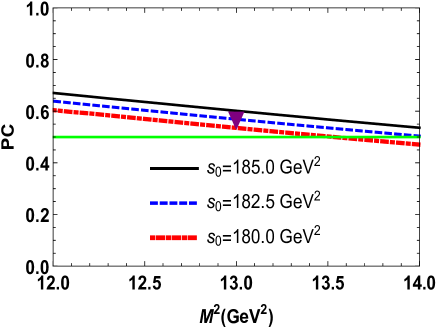
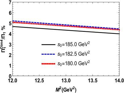
Figure 1: Left: The pole contribution $\mathrm{PC}$ as a function of $M^{2}$. The limit $\mathrm{PC}=0.5$ is shown by the green line. The red triangle shows the point, where the mass $m_{1}$ of the tetraquark $X_{\mathrm{1}}$ has been extracted from the sum rule Right: The ratio $\Pi^{\mathrm{Dim4}}_{1}(M^{2},s_{0})/\Pi_{1}(M^{2},s_{0})$ as a function of the Borel parameter at fixed $s_{0}$.

Computations carried out by employing these constrains prove that the regions

$$M^{2}\in[12,14]~{}\mathrm{GeV}^{2},\ s_{0}\in[180,185]~{}\mathrm{GeV}^{2},$$ (15)

comply with all aforementioned constraints. In fact, at $M^{2}=14~{}\mathrm{GeV}^{2}$ on the average in $s_{0}$ the pole contribution is equal to $\mathrm{PC}\approx 0.5$, whereas at $M^{2}=12~{}\mathrm{GeV}^{2}$ it amounts to $\approx 0.64$. The nonperturbative contribution is positive and at $M^{2}=12~{}\mathrm{GeV}^{2}$ constitutes only $4.5\%$ of the whole result. In Fig. 1 (the left panel), we depict $\mathrm{PC}$ as a function of the Borel parameter at the fixed $s_{0}$. As is seen, excluding only small region for $s_{0}=180~{}\mathrm{GeV}^{2}$ at all values of $M^{2}$ and $s_{0}$ the pole contribution exceeds the $0.5$. The convergence of the $\mathrm{OPE}$ and dominant nature of the perturbative contribution to $\Pi_{1}(M^{2},s_{0})$ is seen in the right panel of the same Fig. 1.

The mass $m_{1}$ and current coupling $\Lambda_{1}$ of the tetraquark $X_{\mathrm{1}}$ are calculated as mean values of these parameters over the regions Eq. (15) and are equal to

$$m_{1} = (12715\pm 80)~{}\mathrm{MeV},$$

$$\Lambda_{1} = (2.80\pm 0.29)~{}\mathrm{GeV}^{5}.$$ (16)

The predictions Eq. (16) correspond to SR results at the point $M^{2}=13~{}\mathrm{GeV}^{2}$ and $s_{0}=182.5~{}\mathrm{GeV}^{2}$, where the pole contribution is $\mathrm{PC}\approx 0.57$. This fact guarantees the dominance of $\mathrm{PC}$ in the obtained results, and proves ground-level nature of the tetraquark $X_{\mathrm{1}}$ in its class. Ambiguities in Eq. (16) are mainly generated by choices of the parameters $M^{2}$ and $s_{0}$. In the case of the mass $m_{1}$ they form only $\pm 0.6\%$ of the obtained result which implies very high accuracy of performed analysis. This fact can be explained by the sum rule for the mass Eq. (11), where it is defined as a ratio of two correlation functions. As a result, variations in correlators are damped in $m_{1}$ which stabilizes numerical output. In the case of $\Lambda_{1}$ ambiguities are equal to $\pm 10\%$ remaining within acceptable limits of SR analysis. The mass $m_{1}$ as a function of $M^{2}$ and $s_{0}$ is plotted in Fig. 2.

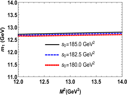
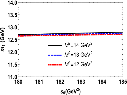
Figure 2: Mass $m_{1}$ of the tetraquark $X_{\mathrm{1}}$ as a function of the Borel parameter $M^{2}$ (left panel), and continuum threshold $s_{0}$ (right panel).

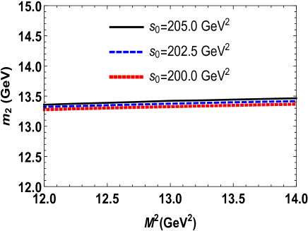
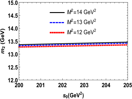
Figure 3: Dependence of the mass $m_{2}$ on the Borel parameter $M^{2}$ (left panel), and continuum threshold parameter $s_{0}$ (right panel).

The mass $m_{2}$ and current coupling $\Lambda_{2}$ of the tetraquark $X_{\mathrm{2}}$ can be analyzed by the similar manner. The only difference here is connected with the QCD side of the SRs. For the current $J_{2}(x)$ the QCD side of the SR is given by the formula

$$\Pi_{2}^{\mathrm{OPE}}(p)=i\int d^{4}xe^{ipx}\left\{\mathrm{Tr}\left[\widetilde{S}_{c}^{a^{\prime}b}(-x)S_{c}^{b^{\prime}a}(-x)\right]\right.$$

$$\times\left[\mathrm{Tr}\left[\widetilde{S}_{b}^{ba^{\prime}}(x)S_{b}^{ab^{\prime}}(x)\right]+\mathrm{Tr}\left[\widetilde{S}_{b}^{aa^{\prime}}(x)S_{b}^{bb^{\prime}}(x)\right]\right]$$

$$+\mathrm{Tr}\left[\widetilde{S}_{c}^{b^{\prime}b}(-x)S_{c}^{a^{\prime}a}(-x)\right]\left[\mathrm{Tr}\left[\widetilde{S}_{b}^{aa^{\prime}}(x)S_{b}^{bb^{\prime}}(x)\right]\right.$$

$$\left.\left.+\mathrm{Tr}\left[\widetilde{S}_{b}^{ba^{\prime}}(x)S_{b}^{ab^{\prime}}(x)\right]\right]\right\}.$$ (17)

The remaining manipulations required to evaluate the $m_{2}$ and $\Lambda_{2}$ do not differ from ones explained above. Therefore, it is convenient to provide final predictions for $m_{2}$ and $\Lambda_{2}$

$$m_{2} = (13370\pm 95)~{}\mathrm{MeV},$$

$$\Lambda_{2} = (1.19\pm 0.14)~{}\mathrm{GeV}^{5},$$ (18)

which are found using the working regions

$$M^{2}\in[12,14]~{}\mathrm{GeV}^{2},\ s_{0}\in[200,205]~{}\mathrm{GeV}^{2},$$ (19)

where all sum rule’s constraints are satisfied. Indeed, the pole contribution on average in $s_{0}$ is larger than $0.5$ for all values of the Borel parameter and changes inside limits

$$0.66\geq\mathrm{PC}\geq 0.51$$ (20)

At $M^{2}=12~{}\mathrm{GeV}^{2}$ the nonperturbative contribution does not exceed $4\%$ of the correlation function. Predictions extracted for the mass $m_{2}$ of the tetraquark $X_{\mathrm{2}}$ are depicted in Fig. 3.

III Full width of the diquark-antidiquark state $X_{\mathrm{1}}$

The masses $m_{1}$ and $m_{2}$ of the scalar tetraquarks $X_{\mathrm{1}}$ and $X_{\mathrm{2}}$ are important parameters to determine their possible decay channels. It is evident that these particles can decay to pair of $\overline{c}b$ mesons with different masses and quantum numbers. Available experimental information on these mesons is restricted by parameters of $B_{c}^{\pm}$ and $B_{c}^{\pm}(2S)$ PDG:2022 . Therefore, to explore decays of $X_{\mathrm{1(2)}}$, we should use also results of theoretical studies. The masses and decay constants of the numerous $\overline{c}b$ mesons were calculated in the framework of different methods. We are going to employ the predictions $m_{B_{c}^{\ast}}=6338~{}\mathrm{MeV}$ and $f_{B_{c}^{\ast}}=471~{}\mathrm{MeV}$ for the mass and decay constant of the vector particles $B_{c}^{\ast\pm}$ from Refs. Godfrey:2004ya and Eichten:2019gig , respectively. It is easy  to see that $m_{1}$ overshoots the thresholds $12549~{}\mathrm{MeV}$ and $12676~{}\mathrm{MeV}$ for production of the pseudoscalar $2B_{c}^{-}$ and vector $2B_{c}^{\ast-}$mesons, respectively. At the same time, the mass of this particle is not enough for the decay $X_{\mathrm{1}}\rightarrow B_{c}^{-}B_{c}^{-}(2S)$ where the mass limit is $13146~{}\mathrm{MeV}$.

III.1 Decay $X_{\mathrm{1}}\rightarrow B_{c}^{-}B_{c}^{-}$

We start from analysis of the process $X_{\mathrm{1}}\rightarrow B_{c}^{-}B_{c}^{-}$. The width of this decay can be computed using the strong coupling $g_{1}$ of particles at the vertex $X_{\mathrm{1}}B_{c}^{-}B_{c}^{-}$. For this purpose, there is a necessity to explore the QCD three-point correlation function

$$\Pi_{1}(p,p^{\prime}) = i^{2}\int d^{4}xd^{4}ye^{ip^{\prime}y}e^{-ipx}\langle 0|\mathcal{T}\{J^{B_{c}}(y)$$ (21)

$$\times J^{B_{c}}(0)J_{1}^{\dagger}(x)\}|0\rangle,$$

where

$$J^{B_{c}}(x)=\overline{c}_{i}(x)i\gamma_{5}b_{i}(x),$$ (22)

is the interpolating current of the pseudoscalar meson $B_{c}^{-}$.

The correlator $\Pi_{1}(p,p^{\prime})$ allows one to find the SR for the strong form factor $g_{1}(q^{2})$, which at the mass shell $q^{2}=m_{B_{c}}^{2}$ gives the coupling $g_{1}$. To derive SR for the form factor $g_{1}(q^{2})$, we follow standard prescriptions of the method and write down $\Pi_{1}(p,p^{\prime})$ using the parameters of the particles involved into the decay process. The correlation function $\Pi_{1}^{\mathrm{Phys}}(p,p^{\prime})$ obtained by this manner constitutes the physical side of the sum rule for the form factor $g_{1}(q^{2})$ and is given by the formula

$$\Pi_{1}^{\mathrm{Phys}}(p,p^{\prime})=\frac{\langle 0|J^{B_{c}}|B_{c}(p^{\prime})\rangle}{p^{\prime 2}-m_{B_{c}}^{2}}\frac{\langle 0|J^{B_{c}}|B_{c}(q)\rangle}{q^{2}-m_{B_{c}}^{2}}$$

$$\times\langle B_{c}(p^{\prime})B_{c}(q)|X_{\mathrm{1}}(p)\rangle\frac{\langle X_{\mathrm{1}}(p)|J_{1}^{\dagger}|0\rangle}{p^{2}-m_{1}^{2}}+\cdots,$$ (23)

where $m_{B_{c}}=(6274.47\pm 0.27)~{}\mathrm{MeV}$ is the mass of $B_{c}^{-}$ meson. The correlator $\Pi_{1}^{\mathrm{Phys}}(p,p^{\prime})$ is found after isolating a contribution of the ground-state particles, whereas effects due to higher states and continuum are denoted by the ellipses. To recast $\Pi_{1}^{\mathrm{Phys}}(p,p^{\prime})$ to easy-to-use form, we employ the matrix element

$$\langle 0|J^{B_{c}}|B_{c}\rangle=\frac{f_{B_{c}}m_{B_{c}}^{2}}{m_{b}+m_{c}},$$ (24)

with $f_{B_{c}}=(476\pm 27)~{}\mathrm{MeV}$ being the decay constant of the meson $B_{c}^{\pm}$ Veliev:2010vd . We also model the vertex $X_{\mathrm{1}}B_{c}B_{c}$ using the expression

$$\langle B_{c}(p^{\prime})B_{c}(q)|X_{\mathrm{1}}(p)\rangle=g_{1}(q^{2})p\cdot p^{\prime}.$$ (25)

Then, the correlation function (23) can be presented in the following form

$$\Pi_{1}^{\mathrm{Phys}}(p,p^{\prime})=g_{1}(q^{2})\frac{\Lambda_{1}f_{B_{c}}^{2}m_{B_{c}}^{4}}{(m_{b}+m_{c})^{2}\left(p^{2}-m_{1}^{2}\right)}$$

$$\times\frac{m_{1}^{2}+m_{B_{c}}^{2}-q^{2}}{2\left(p^{\prime 2}-m_{B_{c}}^{2}\right)(q^{2}-m_{B_{c}}^{2})}+\cdots.$$ (26)

Because $\Pi_{1}^{\mathrm{Phys}}(p,p^{\prime})$ has a simple Lorentz structure proportional to $\mathrm{I}$, we denote by $\Pi_{1}^{\mathrm{Phys}}(p^{2},p^{\prime 2},q^{2})$ the right-hand side of Eq. (26) as the invariant amplitude and use it to derive SR for $g_{1}(q^{2})$.

The QCD side of SR is equal to

$$\Pi_{1}^{\mathrm{OPE}}(p,p^{\prime})=2i^{2}\int d^{4}xd^{4}ye^{ip^{\prime}y}e^{-ipx}\left\{\mathrm{Tr}\left[\gamma_{5}S_{b}^{ib}(y-x)\right.\right.$$

$$\left.\times\gamma_{\mu}\widetilde{S}_{b}^{ja}(-x)\gamma_{5}\widetilde{S}_{c}^{bj}(x)\gamma^{\mu}S_{c}^{ai}(x-y)\right]$$

$$\left.-\mathrm{Tr}\left[\gamma_{5}S_{b}^{ib}(y-x)\gamma_{\mu}\widetilde{S}_{b}^{ja}(-x){}\gamma_{5}\widetilde{S}_{c}^{aj}(x)\gamma^{\mu}S_{c}^{bi}(x-y)\right]\right\}.$$

(27)

The $\Pi_{1}^{\mathrm{OPE}}(p,p^{\prime})$ has also a trivial Lorentz structure, and $\Pi_{1}^{\mathrm{OPE}}(p^{2},p^{\prime 2},q^{2})$ stands for the corresponding amplitude. Then, the SR for the form factor $g_{1}(q^{2})$ reads

$$g_{1}(q^{2})=\frac{2(m_{b}+m_{c})^{2}}{\Lambda_{1}f_{B_{c}}^{2}m_{B_{c}}^{4}}\frac{q^{2}-m_{B_{c}}^{2}}{m^{2}+m_{B_{c}}^{2}-q^{2}}$$

$$\times e^{m_{1}^{2}/M_{1}^{2}}e^{m_{B_{c}}^{2}/M_{2}^{2}}\Pi_{1}(\mathbf{M}^{2},\mathbf{s}_{0},q^{2}).$$ (28)

Here,

$$\Pi_{1}(\mathbf{M}^{2},\mathbf{s}_{0},q^{2})=\int_{4\mathcal{M}^{2}}^{s_{0}}ds\int_{\mathcal{M}^{2}}^{s_{0}^{\prime}}ds^{\prime}\rho_{1}(s,s^{\prime},q^{2})$$

$$\times e^{-s/M_{1}^{2}}e^{-s^{\prime}/M_{2}^{2}}.$$ (29)

is the function $\Pi_{1}^{\mathrm{OPE}}(p^{2},p^{\prime 2},q^{2})$ undergone Borel transformations and continuum subtractions. It is written in term of the spectral density $\rho(s,s^{\prime},q^{2})$. In Eq. (28) $\mathbf{M}^{2}=(M_{1}^{2},M_{2}^{2})$ and $\mathbf{s}_{0}=(s_{0},s_{0}^{\prime})$ are the Borel and continuum threshold parameters, respectively.

To carry out numerical computations, we use for $M_{1}^{2}$ and $s_{0}$, associated with the $X_{\mathrm{1}}$ channel, the regions from Eq. (15). The parameters $(M_{2}^{2},\ s_{0}^{\prime})$ for the $B_{c}^{-}$ meson channel are changed within the limits

$$M_{2}^{2}\in[6.5,7.5]~{}\mathrm{GeV}^{2},\ s_{0}^{\prime}\in[45,47]~{}\mathrm{GeV}^{2}.$$ (30)

The SR approach generates reliable predictions for the form factor $g_{1}(q^{2})$ in the Euclidean region $q^{2}<0$. But the strong coupling $g_{1}$should be determined at the mass shell $q^{2}=m_{B_{c}}^{2}$. To evade this obstacle, it is appropriate to introduce a new variable $Q^{2}=-q^{2}$ and use $g_{1}(Q^{2})$ for the obtained function. Afterwards, we employ a function $\mathcal{F}_{1}(Q^{2})$ that at momenta $Q^{2}>0$ generates values coinciding with the SR predictions, but can be extrapolated to the region of $Q^{2}<0$. For these purposes, we employ the functions $\mathcal{F}_{i}(Q^{2},m_{1}^{2})$

$$\mathcal{F}_{i}(Q^{2},m_{1}^{2})=\mathcal{F}_{i}^{0}\mathrm{\exp}\left[c_{i}^{1}\frac{Q^{2}}{m_{1}^{2}}+c_{i}^{2}\left(\frac{Q^{2}}{m_{1}^{2}}\right)^{2}\right]$$ (31)

with parameters $\mathcal{F}_{i}^{0}$, $c_{i}^{1}$, and $c_{i}^{2}$.

In our present analysis, SR calculations comprise $Q^{2}$ from the interval $Q^{2}=1\div 10~{}\mathrm{GeV}^{2}$. Results of relevant computations are plotted in Fig. 4. It is easy to fix the parameters $\mathcal{F}_{1}^{0}=0.41~{}\mathrm{GeV}^{-1}$, $c_{1}^{1}=4.13$, and $c_{1}^{2}=0.31$ of the function $\mathcal{F}_{1}(Q^{2},m_{1}^{2})$ which leads to reasonable agreement with the SR data: This function is shown in Fig. 4 as well.

Then, for the strong coupling $g_{1}$, we get

$$g_{1}\equiv\mathcal{F}_{1}(-m_{B_{c}}^{2},m_{1}^{2})=(1.7\pm 0.3)\times 10^{-1}\ \mathrm{GeV}^{-1}.$$ (32)

The width of the process $X_{\mathrm{1}}\rightarrow B_{c}^{-}B_{c}^{-}$ is given by the formula

$$\Gamma\left[X_{\mathrm{1}}\rightarrow B_{c}^{-}B_{c}^{-}\right]=g_{1}^{2}\frac{m_{B_{c}}^{2}\lambda_{1}}{8\pi}\left(1+\frac{\lambda_{1}^{2}}{m_{B_{c}}^{2}}\right),$$ (33)

where $\lambda_{1}=\lambda(m_{1},m_{B_{c}},m_{B_{c}})$, and

$$\lambda(x,y,z)=\frac{\sqrt{x^{4}+y^{4}+z^{4}-2(x^{2}y^{2}+x^{2}z^{2}+y^{2}z^{2})}}{2x}.$$ (34)

As a result, we obtain

$$\Gamma\left[X_{\mathrm{1}}\rightarrow B_{c}^{-}B_{c}^{-}\right]=(38.3\pm 9.8)~{}\mathrm{MeV}.$$ (35)

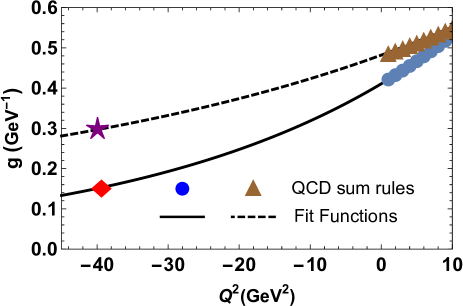
Figure 4: QCD data and fit functions for the form factors $g_{1}(Q^{2})$ (solid line) and $g_{2}(Q^{2})$ (dashed line). The diamond on the solid line and star on the dashed curve fix the points $Q^{2}=-m_{B_{c}}^{2}$ and $Q^{2}=-m_{B_{c}^{\ast}}^{2}$ where $g_{1}$ and $g_{2}$ have been extracted.

III.2 Process $X_{\mathrm{1}}\rightarrow B_{c}^{\ast-}B_{c}^{\ast-}$

The decay $X_{\mathrm{1}}\rightarrow B_{c}^{\ast-}B_{c}^{\ast-}$ is $S$-wave process, partial width of which is determined by the strong coupling $g_{2}$ at the vertex $X_{\mathrm{1}}B_{c}^{\ast-}B_{c}^{\ast-}$. In the context of the QCD SR method the form factor $g_{2}(q^{2})$ is calculated using the three-point correlation function

$$\Pi_{\mu\nu}(p,p^{\prime})=i^{2}\int d^{4}xd^{4}ye^{ip^{\prime}y}e^{-ipx}\langle 0|\mathcal{T}\{J_{\mu}^{B_{c}^{\ast}}(y)$$

$$\times J_{\nu}^{B_{c}^{\ast}}(0)J_{1}^{\dagger}(x)\}|0\rangle,$$ (36)

with $J_{\mu}^{B_{c}^{\ast}}(x)$ being the interpolating current for the vector meson $B_{c}^{\ast-}$

$$J_{\mu}^{B_{c}^{\ast}}(x)=\overline{c}_{i}(x)\gamma_{\mu}b_{i}(x).$$ (37)

Here, $p$, $p^{\prime}$, and $q=p-p^{\prime}$ are $4$-momenta of the tetraquark $X_{\mathrm{1}}(p)$, and $B_{c}^{\ast-}(p^{\prime})$, $B_{c}^{\ast-}(q)$ mesons, respectively.

To compute the phenomenological side of the SR, we need the following matrix elements

$$\langle 0|J_{\mu}^{B_{c}^{\ast}}|B_{c}^{\ast}(p)\rangle=f_{B_{c}^{\ast}}m_{B_{c}^{\ast}}\varepsilon_{\mu}(p),$$ (38)

and

$$\langle B_{c}^{\ast}(p^{\prime})B_{c}^{\ast}(q)|X_{\mathrm{1}}(p)\rangle=g_{2}(q^{2})\left[q\cdot p^{\prime}\varepsilon^{\ast}(p^{\prime})\cdot\varepsilon^{\ast}(q)\right.$$

$$\left.-q\cdot\varepsilon^{\ast}(p^{\prime})p^{\prime}\cdot\varepsilon^{\ast}(q)\right],$$ (39)

where $\varepsilon(p^{\prime})$ and $\varepsilon(q)$ are the polarization vectors of $B_{c}^{\ast-}(p^{\prime})$, and $B_{c}^{\ast-}(q)$.

After some computations, we get for the physical side of the sum rule

$$\Pi_{\mu\nu}^{\mathrm{Phys}}(p,p^{\prime})=g_{2}(q^{2})\frac{\Lambda_{1}f_{B_{c}^{\ast}}^{2}m_{B_{c}^{\ast}}^{2}}{\left(p^{2}-m_{1}^{2}\right)\left(p^{\prime 2}-m_{B_{c}^{\ast}}^{2}\right)(q^{2}-m_{B_{c}^{\ast}}^{2})}$$

$$\times\left[\frac{1}{2}\left(m_{1}^{2}-m_{B_{c}^{\ast}}^{2}-q^{2}\right)g_{\mu\nu}-q_{\mu}p_{\nu}^{\prime}\right]+\cdots.$$ (40)

The correlator $\Pi_{\mu\nu}^{\mathrm{Phys}}(p,p^{\prime})$ contains two Lorentz structures that can be used to obtain the SR for $g_{2}(q^{2})$. We select to work with the contribution $\sim g_{\mu\nu}$ and present the corresponding invariant amplitude as $\widehat{\Pi}_{1}^{\mathrm{Phys}}(p^{2},p^{\prime 2},q^{2})$. The Borel transformations of the amplitude $\widehat{\Pi}_{1}^{\mathrm{Phys}}(p^{2},p^{\prime 2},q^{2})$ over $-p^{2}$ and $-p^{\prime 2}$ yield

$$\mathcal{B}\widehat{\Pi}_{1}^{\mathrm{Phys}}(p^{2},p^{\prime 2},q^{2})=g_{2}(q^{2})\Lambda_{1}f_{B_{c}^{\ast}}^{2}m_{B_{c}^{\ast}}^{2}$$

$$\times\frac{m_{1}^{2}-m_{B_{c}^{\ast}}^{2}-q^{2}}{2(q^{2}-m_{B_{c}^{\ast}}^{2})}e^{-m_{1}^{2}/M_{1}^{2}}e^{-m_{B_{c}^{\ast}}^{2}/M_{2}^{2}}+\cdots.$$ (41)

The correlation function $\Pi_{\mu\nu}(p,p^{\prime})$ expressed in terms of $c$-quark propagators reads

$$\Pi_{\mu\nu}^{\mathrm{OPE}}(p,p^{\prime})=2i^{2}\int d^{4}xd^{4}ye^{ip^{\prime}y}e^{-ipx}\left\{\mathrm{Tr}\left[\gamma_{\mu}S_{b}^{ib}(y-x)\right.\right.$$

$$\left.\times\gamma_{\theta}\widetilde{S}_{b}^{ja}(-x){}\gamma_{\nu}\widetilde{S}_{c}^{bj}(x)\gamma^{\theta}S_{c}^{ai}(x-y)\right]$$

$$\left.-\mathrm{Tr}\left[\gamma_{\mu}S_{b}^{ib}(y-x)\gamma_{\theta}\widetilde{S}_{b}^{ja}(-x){}\gamma_{\nu}\widetilde{S}_{c}^{aj}(x)\gamma^{\theta}S_{c}^{bi}(x-y)\right]\right\}.$$

(42)

The invariant amplitude $\widehat{\Pi}_{1}^{\mathrm{OPE}}(p^{2},p^{\prime 2},q^{2})$ corresponding to the component $\sim g_{\mu\nu}$ in Eq. (42) forms the QCD side of the SR.

Having equated amplitudes $\widehat{\Pi}_{1}^{\mathrm{OPE}}(p^{2},p^{\prime 2},q^{2})$ and $\widehat{\Pi}_{1}^{\mathrm{Phys}}(p^{2},p^{\prime 2},q^{2})$ and performed the doubly Borel transforms and continuum subtractions, one can find the sum rule for the form factor $g_{2}(q^{2})$

$$g_{2}(q^{2})=\frac{2}{\Lambda_{1}f_{B_{c}^{\ast}}^{2}m_{B_{c}^{\ast}}^{2}}\frac{q^{2}-m_{B_{c}^{\ast}}^{2}}{m_{1}^{2}-m_{B_{c}^{\ast}}^{2}-q^{2}}$$

$$\times e^{m_{1}^{2}/M_{1}^{2}}e^{m_{B_{c}^{\ast}}^{2}/M_{2}^{2}}\widehat{\Pi}_{1}(\mathbf{M}^{2},\mathbf{s}_{0},q^{2}).$$ (43)

The remaining manipulations do not differ considerably from ones described above. Therefore, let us write down the region for parameters $M_{2}^{2}$, and $s_{0}^{\prime}$ in the channel of $B_{c}^{\ast-}$ meson

$$M_{2}^{2}\in[6.5,7.5]~{}\mathrm{GeV}^{2},\ s_{0}^{\prime}\in[49,51]~{}\mathrm{GeV}^{2}.$$ (44)

The extrapolating function $\mathcal{F}_{2}(Q^{2},m_{1}^{2})$ has the parameters: $\mathcal{F}_{2}^{0}=0.48~{}\mathrm{GeV}^{-1}$, $c_{2}^{1}=2.14$, and $c_{2}^{2}=0.74$. Then, the strong coupling $g_{2}$ is equal to

$$g_{2}\equiv\mathcal{F}_{2}(-m_{B_{c}^{\ast}}^{2},m_{1}^{2})=(3.0\pm 0.4)\times 10^{-1}\ \mathrm{GeV}^{-1}.$$ (45)

The width of the decay $X_{\mathrm{1}}\rightarrow B_{c}^{\ast-}B_{c}^{\ast-}$ can be evaluated by means of the expression

$$\Gamma\left[X_{\mathrm{1}}\rightarrow B_{c}^{\ast-}B_{c}^{\ast-}\right]=g_{2}^{2}\frac{\lambda_{2}}{8\pi}\left(\frac{m_{B_{c}^{\ast}}^{4}}{m_{1}^{2}}+\frac{2\lambda_{2}^{2}}{3}\right),$$ (46)

where $\lambda_{2}=\lambda(m_{1},m_{B_{c}^{\ast}},m_{B_{c}^{\ast}})$.

Having used Eq. (46) and the strong coupling $g_{2}$, we find

$$\Gamma\left[X_{\mathrm{1}}\rightarrow B_{c}^{\ast-}B_{c}^{\ast-}\right]=(24.3\pm 6.2)~{}\mathrm{MeV}.$$ (47)

Two processes considered in this section form the full width of the tetraquark $X_{\mathrm{1}}$ which amounts to

$$\Gamma_{\mathrm{1}}=(63\pm 12)~{}\mathrm{MeV}.$$ (48)

IV Full width of the tetraquark $X_{\mathrm{2}}$

The prediction for the mass $m_{2}=13370~{}\mathrm{MeV}$ of the state $X_{\mathrm{2}}$ demonstrates that it is considerably heavier than $X_{\mathrm{1}}$. As a result, $X_{\mathrm{2}}$ can decay to $2B_{c}^{-}$, and $2B_{c}^{\ast-}$ mesons, but its mass is also enough for the process $X_{\mathrm{2}}\rightarrow B_{c}^{-}B_{c}^{-}(2S)$ with the mass threshold of $13146~{}\mathrm{MeV}$.

IV.1 $X_{\mathrm{2}}\rightarrow B_{c}^{-}B_{c}^{-}$ and $X_{\mathrm{2}}\rightarrow B_{c}^{-}B_{c}^{-}(2S)$

Because the mesons $B_{c}^{-}$ and $B_{c}^{-}(2S)$ are described by the same interpolating current these two decays should be treated in a correlated form. The correlation function required to extract the strong form factors $G_{1}(q^{2})$ and $G_{2}(q^{2})$ at the vertices $X_{\mathrm{2}}B_{c}^{-}B_{c}^{-}$ and $X_{\mathrm{2}}B_{c}^{-}B_{c}^{-}(2S)$ is given by the expression

$$\Pi_{2}(p,p^{\prime}) = i^{2}\int d^{4}xd^{4}ye^{ip^{\prime}y}e^{-ipx}\langle 0|\mathcal{T}\{J^{B_{c}}(y)$$ (49)

$$\times J^{B_{c}}(0)J_{2}^{\dagger}(x)\}|0\rangle.$$

The phenomenological side of SRs for these form factors is determined by the formula

$$\Pi_{2}^{\mathrm{Phys}}(p,p^{\prime})=G_{1}(q^{2})\frac{\Lambda_{2}f_{B_{c}}^{2}m_{B_{c}}^{4}}{(m_{b}+m_{c})^{2}\left(p^{2}-m_{2}^{2}\right)}$$

$$\times\frac{m_{2}^{2}+m_{B_{c}}^{2}-q^{2}}{2\left(p^{\prime 2}-m_{B_{c}}^{2}\right)(q^{2}-m_{B_{c}}^{2})}$$

$$+G_{2}(q^{2})\frac{\Lambda_{2}\widetilde{f}_{B_{c}}\widetilde{m}_{B_{c}}^{2}f_{B_{c}}m_{B_{c}}^{2}}{(m_{b}+m_{c})^{2}\left(p^{2}-m_{2}^{2}\right)}$$

$$\times\frac{m_{2}^{2}+\widetilde{m}_{B_{c}}^{2}-q^{2}}{2\left(p^{\prime 2}-\widetilde{m}_{B_{c}}^{2}\right)(q^{2}-m_{B_{c}}^{2})}+\cdots,$$ (50)

where $\widetilde{m}_{B_{c}}=(6871.2\pm 1.0)~{}\mathrm{MeV}$ and $\widetilde{f}_{B_{c}}=(420\pm 20)~{}\mathrm{MeV}$ are the mass and decay constant of the radially excited meson $B_{c}^{-}(2S)$ from Refs. PDG:2022 and Aliev:2019wcm , respectively.

The second component of the sum rules, i.e., the correlation function $\Pi_{2}(p,p^{\prime})$ in terms of quark propagators takes the following form:

$$\Pi_{2}^{\mathrm{OPE}}(p,p^{\prime})=2i^{2}\int d^{4}xd^{4}ye^{ip^{\prime}y}e^{-ipx}\left\{\mathrm{Tr}\left[\gamma_{5}S_{b}^{ib}(y-x)\right.\right.$$

$$\left.\times\widetilde{S}_{b}^{ja}(-x)\gamma_{5}\widetilde{S}_{c}^{aj}(x)S_{c}^{bi}(x-y)\right]$$

$$\left.+\mathrm{Tr}\left[\gamma_{5}S_{b}^{ib}(y-x)\widetilde{S}_{b}^{ja}(-x){}\gamma_{5}\widetilde{S}_{c}^{bj}(x)S_{c}^{ai}(x-y)\right]\right\}.$$

(51)

Functions $\Pi_{2}^{\mathrm{Phys}}(p,p^{\prime})$ and $\Pi_{2}^{\mathrm{OPE}}(p,p^{\prime})$ have trivial Lorentz structures. Having denoted corresponding invariant amplitudes by $\Pi_{2}^{\mathrm{Phys}}(p^{2},p^{\prime 2},q^{2})$ and $\Pi_{2}^{\mathrm{OPE}}(p^{2},p^{\prime 2},q^{2})$, equated them to each other and carried out usual operations, it is possible to derive the required SR equality for the form factors $G_{1}(q^{2})$ and $G_{2}(q^{2})$.

An expression obtained by this way depends on two unknown functions $G_{1}(q^{2})$ and $G_{2}(q^{2})$. We solve this problem gradually: At the first step, we consider the form factor $G_{1}(q^{2})$, and use it at the next stage to determine $G_{2}(q^{2})$. These two stages differ from each another by a choice of the regions for the parameters $(M_{2}^{2},s_{0}^{\prime})$. At the first phase of analysis, we restrict $s_{0}^{\prime}$ by the mass of the orbitally excited meson $B_{c}^{-}(2S)$ choosing $s_{0}^{\prime}<\widetilde{m}_{B_{c}}^{2}$. This enable us to include contribution of the vertex $X_{\mathrm{2}}B_{c}^{-}B_{c}^{-}(2S)$ into the ”continuum” and consider only the first term in Eq. (50). The relevant parameters $(M_{2}^{2},s_{0}^{\prime})$ are given in Eq. (30).

At the next step, we fix

$$M_{2}^{2}\in[6.5,7.5]~{}\mathrm{GeV}^{2}\text{, }s_{0}^{\ast^{\prime}}\in[48,50]~{}\mathrm{GeV}^{2},$$ (52)

and use $G_{1}(q^{2})$ as input information to extract the form factor $G_{2}(q^{2})$, where $s_{0}^{\ast^{\prime}}$ is less than $m^{2}[B_{c}(3S)]=(7.272)^{2}~{}\mathrm{GeV}^{2}$ Godfrey:2004ya . In both steps for $(M_{1}^{2},s_{0})$ we employ the parameters from Eq. (19).

Analysis performed in the framework of this approach leads to the results

$$G_{1}\equiv\mathcal{G}_{1}(-m_{B_{c}}^{2},m_{2}^{2})=(1.1\pm 0.2)\times 10^{-1}\ \mathrm{GeV}^{-1},$$ (53)

and

$$G_{2}\equiv\mathcal{G}_{2}(-m_{B_{c}}^{2},m_{2}^{2})=(0.7\pm 0.1)\times 10^{-1}\ \mathrm{GeV}^{-1},$$ (54)

where $\mathcal{G}_{i}(Q^{2}$,$m_{2}^{2})$ have the same analytic form as $\mathcal{F}_{i}(Q^{2}$,$m_{1}^{2})$ but with substitution $m_{1}^{2}\rightarrow m_{2}^{2}$. Let us note that though the couplings $G_{1}$ and $G_{2}$ are determined at the mass shell of the $B_{c}^{-}$ meson, due to fitting parameters $\mathcal{G}_{1}$ and $\mathcal{G}_{2}$ are different functions.

The width of the decays $X_{\mathrm{2}}\rightarrow B_{c}^{-}B_{c}^{-}$ and $X_{\mathrm{2}}\rightarrow B_{c}^{-}B_{c}^{-}(2S)$ can be computed using Eq. (33) after relevant replacements

$$\Gamma\left[X_{\mathrm{2}}\rightarrow B_{c}^{-}B_{c}^{-}\right]=(45.5\pm 11.7)~{}\mathrm{MeV},$$

$$\Gamma\left[X_{\mathrm{2}}\rightarrow B_{c}^{-}B_{c}^{-}(2S)\right]=(11.9\pm 2.8)~{}\mathrm{MeV}.$$ (55)

IV.2 $X_{\mathrm{2}}\rightarrow B_{c}^{\ast-}B_{c}^{\ast-}$

We are going to analyze the decay $X_{\mathrm{2}}\rightarrow B_{c}^{\ast-}B_{c}^{\ast-}$ by means of the correlation function

$$\widetilde{\Pi}_{\mu\nu}(p,p^{\prime}) = i^{2}\int d^{4}xd^{4}ye^{ip^{\prime}y}e^{-ipx}\langle 0|\mathcal{T}\{J_{\mu}^{B_{c}^{\ast}}(y)$$ (56)

$$\times J_{\nu}^{B_{c}^{\ast}}(0)J_{2}^{\dagger}(x)\}|0\rangle.$$

Using the parameters $m_{2}$, $\Lambda_{2}$ and $f_{B_{c}^{\ast}}$, $m_{B_{c}^{\ast}}$, one can recast the correlator $\widetilde{\Pi}_{\mu\nu}(p,p^{\prime})$ into the form

$$\widetilde{\Pi}_{\mu\nu}^{\mathrm{Phys}}(p,p^{\prime})=\frac{G_{3}(q^{2})\Lambda_{2}f_{B_{c}^{\ast}}^{2}m_{B_{c}^{\ast}}^{2}}{\left(p^{2}-m_{2}^{2}\right)\left(p^{\prime 2}-m_{B_{c}^{\ast}}^{2}\right)(q^{2}-m_{B_{c}^{\ast}}^{2})}$$

$$\times\left[\frac{1}{2}\left(m_{2}^{2}-m_{B_{c}^{\ast}}^{2}-q^{2}\right)g_{\mu\nu}-q_{\mu}p_{\nu}^{\prime}\right]+\cdots,$$ (57)

where $G_{3}(q^{2})$ is the strong form factor of interest. Evidently, $\widetilde{\Pi}_{\mu\nu}^{\mathrm{Phys}}(p,p^{\prime})$ can be used to extract the invariant amplitude necessary for our purposes. We work with the Lorentz structure $g_{\mu\nu}$, therefore relevant part of $\widetilde{\Pi}_{\mu\nu}^{\mathrm{Phys}}(p,p^{\prime})$ constitutes the physical side of SR. The sum rule’s QCD side is determined by the function

$$\widetilde{\Pi}_{\mu\nu}^{\mathrm{OPE}}(p,p^{\prime})=2i^{2}\int d^{4}xd^{4}ye^{ip^{\prime}y}e^{-ipx}\left\{\mathrm{Tr}\left[\gamma_{\mu}S_{b}^{ib}(y-x)\right.\right.$$

$$\left.\times\widetilde{S}_{b}^{ja}(-x){}\gamma_{\nu}\widetilde{S}_{c}^{bj}(x)S_{c}^{ai}(x-y)\right]$$

$$\left.+\mathrm{Tr}\left[\gamma_{\mu}S_{b}^{ib}(y-x)\widetilde{S}_{b}^{ja}(-x){}\gamma_{\nu}\widetilde{S}_{c}^{aj}(x)S_{c}^{bi}(x-y)\right]\right\}.$$ (58)

Having omitted further details, we write down the final results for the parameters of this decay:

$$G_{3}\equiv\mathcal{G}_{3}(-m_{B_{c}^{\ast}}^{2},m_{2}^{2})=(1.4\pm 0.3)\times 10^{-1}\ \mathrm{GeV}^{-1},$$ (59)

and

$$\Gamma\left[X_{\mathrm{2}}\rightarrow B_{c}^{\ast-}B_{c}^{\ast-}\right]=(21.3\pm 6.5)~{}\mathrm{MeV}.$$ (60)

Then, the full width of the tetraquark $X_{\mathrm{2}}$ is

$$\Gamma_{2}=(79\pm 14)~{}\mathrm{MeV}.$$ (61)

V Analysis and conclusions

In present work, we have investigated the doubly charged scalar diquark-antidiquark states $X_{\mathrm{1}}$ and $X_{\mathrm{2}}$ with the axial-vector and pseudoscalar ingredients, respectively. The tetraquark $X_{\mathrm{1}}$ is the $\overline{\mathbf{3}_{c}}\otimes\mathbf{3}_{c}$ color state, and is expected to occupy one of a lowest level in the spectroscopy of similar exotic mesons. The second diquark-antidiquark state $X_{\mathrm{2}}$ studied here has the same quantum numbers, but different inner structure: it is built of color-sextet diquarks $\mathbf{6}_{c}\otimes\overline{\mathbf{6}}_{c}$.

The mass $m_{1}=(12715\pm 80)~{}\mathrm{MeV}$ of $X_{\mathrm{1}}$ is considerably smaller than the mass of the structure $X_{\mathrm{2}}$. But $m_{1}$ does not ensures strong-interaction stability of the tetraquark $X_{\mathrm{1}}$. It turns out that $X_{\mathrm{1}}$ can decay to pairs of $B_{c}^{-}B_{c}^{-}$ and $B_{c}^{\ast-}B_{c}^{\ast-}$ mesons. These channels form the full width $\Gamma_{\mathrm{1}}=(63\pm 12)~{}\mathrm{MeV}$ of the state $X_{\mathrm{1}}$ which characterizes it as a ”typical” tetraquark with the relatively modest width. The tetraquark $X_{\mathrm{2}}$ has the mass $m_{2}=(13370\pm 95)~{}\mathrm{MeV}$ and width $\Gamma_{\mathrm{2}}=(79\pm 14)~{}\mathrm{MeV}$, and is also unstable particle from a family of doubly charged heavy diquak-antidiquark states.

The tetraquarks $X_{\mathrm{1}}$ and $X_{\mathrm{2}}$ are ”pure” diquark-antidiquark states with fixed internal organizations. In general, there are other options to model scalar particle $bb\overline{c}\overline{c}$ Wang:2021taf . Thus, the scalar tetraquark $bb\overline{c}\overline{c}$ can also have structures $C\gamma_{5}\otimes\gamma_{5}C$, $C\gamma_{\mu}\gamma_{5}\otimes\gamma^{\mu}\gamma_{5}C$ and $C\sigma_{\mu\nu}\otimes\sigma^{\mu\nu}C$. First two models are composed of color sextet diquarks, whereas the last one belongs to the triplet representation of the color group. If exist, scalar tetraquarks $bb\overline{c}\overline{c}$ may have the same mass and width as aforementioned five basic diquark-antidiquark states. A physical particle alternatively may be an admixture of these basic states. But identifications of real scalar four-quark mesons $bb\overline{c}\overline{c}$ as mixed states, calculations corresponding mixing parameters are possible only after measuring their physical parameters.

Nevertheless, even in the lack of such experimental information, we can make some conclusions about importance of one or the other basic component in a ground-level scalar particle $bb\overline{c}\overline{c}$. For these purposes, it is useful to consider an overlap of the currents $J_{1}(x)$ and $J_{2}(x)$ with the physical state determined by matrix elements $\langle 0|J|X\rangle=\Lambda$

$$\Lambda_{1} = (2.80\pm 0.29)~{}\mathrm{GeV}^{5},$$

$$\Lambda_{2} = (1.19\pm 0.14)~{}\mathrm{GeV}^{5}.$$ (62)

Because $\Lambda_{1}>\Lambda_{2}$, the scalar diquark-antidiquark state couples with a larger strength to the current $J_{1}(x)$ than to $J_{2}(x)$. In other words, in the ground-level scalar particle, the axial-axial state $C\gamma_{\mu}\otimes\gamma^{\mu}C$ with smaller mass is a dominant component. Comprehensive analysis of relevant problems requires experimental data and theoretical analysis of another basic states, which are beyond the scope of the present article.

As we have mentioned above, tetraquarks $bb\overline{c}\overline{c}$/$cc\overline{b}\overline{b}$ were explored in numerous articles using different methods. The main problem considered in these publications was calculation of their masses and looking for particles stable against strong decays. Thus, the mass of scalar states $bb\overline{c}\overline{c}$/$cc\overline{b}\overline{b}$ in a color-magnetic-interaction model was estimated within the limits $12571\div 12597~{}\mathrm{MeV}$, which is lower than our prediction for $X_{\mathrm{1}}$ but still higher than the $2B_{c}^{-}$ threshold Wu:2016vtq .

The scalar tetraquarks $bb\overline{c}\overline{c}$ with both the color triplet and sextet organizations were studied in Ref. Wang:2019rdo in the framework of nonrelativistic quark models. The mass of $bb\overline{c}\overline{c}$ in the model I was found equal to $12863~{}\mathrm{MeV}$ for $\overline{\mathbf{3}_{c}}\otimes\mathbf{3}_{c}$ configuration and to $12850~{}\mathrm{MeV}$ in the case of $\mathbf{6}_{c}\otimes\overline{\mathbf{6}}_{c}$ structure. The model II led to slightly higher results: $12915~{}\mathrm{MeV}$ and $12919~{}\mathrm{MeV}$, respectively. In any case, these states are above the open heavy-flavor thresholds. Parameters of fully heavy tetraquarks including $bb\overline{c}\overline{c}$/$cc\overline{b}\overline{b}$ ones were also considered in Ref. Liu:2019zuc in the context of the potential model by including the linear confining and Coulomb potentials, as well as spin-spin interactions. It was found that there are two scalar tetraquarks $bb\overline{c}\overline{c}$ which are admixtures of the color triplet and sextet states. In the particle with the mass $13039~{}\mathrm{MeV}$ the dominant component is the sextet state, whereas in the second one with the mass $12947~{}\mathrm{MeV}$ prevails the triplet constituent. Both of these states are unstable against strong decays, and through quark rearrangement can easily dissociate to open-flavor mesons with appropriate quantum numbers.

Interesting predictions concerning diquark-antidiquark states $bb\overline{c}\overline{c}$ were made in Ref. Wang:2021taf , in which the masses of the scalar tetraquarks with triplet and sextet compositions were estimated as $12330_{-150}^{+180}~{}\mathrm{MeV}$ and $13320_{-240}^{+300}~{}\mathrm{MeV}$, respectively. In accordance with this paper, the state $\overline{\mathbf{3}_{c}}\otimes\mathbf{3}_{c}$ is below the $2B_{c}^{-}$ threshold and is strong-interaction stable tetraquark, whereas the mass of the structure $\mathbf{6}_{c}\otimes\overline{\mathbf{6}}_{c}$ overshoots this limit.

As is seen, unstable nature of the scalar tetraquarks $X_{\mathrm{1}}$ and $X_{\mathrm{2}}$ was confirmed almost in all publications. Only in Ref. Wang:2021taf the scalar particle $X_{\mathrm{1}}$ (and some other tetraquarks) was found stable against strong decays. Our prediction for $m_{1}$ is considerably higher than $12330_{-150}^{+180}~{}\mathrm{MeV}$, whereas the result for the mass $m_{2}$ of the state $X_{\mathrm{2}}$ nicely agrees with one from Ref. Wang:2021taf . Additionally, though our prediction for the mass splitting $\approx 650~{}\mathrm{MeV}$ between the states $X_{\mathrm{1}}$ and $X_{\mathrm{2}}$ is smaller than a gap obtained there, it is qualitatively consistent with it: In other publications mentioned above, this splitting is very small.

The widths of the particles $X_{\mathrm{1}}$ and $X_{\mathrm{2}}$ allow us to interpret them as relatively narrow tetraquarks. The full width of scalar tetraquark $bb\overline{c}\overline{c}$ was evaluated in Ref. Li:2019uch as well. To this end, the authors used its weak semileptonic and non-leptonic decays, and estimated the width and lifetime of this structure as $(3.97\pm 1.50)\times 10^{-9}\ \mathrm{MeV}$ and $(0.17\pm 0.02)\times 10^{-12}\ \mathrm{s}$, respectively. If the tetraquark $X_{\mathrm{1}}$ was strong-interaction stable particle, this information would be very important to search for it in various processes. But, widths $X_{\mathrm{1}}$ and $X_{\mathrm{2}}$ amount to a few $\mathrm{MeV}$, therefore contributions of weak decays to the corresponding parameters are negligible.

There are numerous problems in physics of fully heavy tetraquarks waiting for their solution. Only relevant experimental measurements combined with theoretical studies of different four-quark structures can fill up this segment of exotic hadron spectroscopy.

References

- (1) R. Aaij et al. (LHCb Collaboration), Sci. Bull. 65, 1983 (2020).
- (2) E. Bouhova-Thacker (ATLAS Collaboration), PoS ICHEP2022, 806 (2022).
- (3) A. Hayrapetyan, et al. (CMS Collaboration) arXiv:2306.07164 [hep-ex].
- (4) S. S. Agaev, K. Azizi, B. Barsbay, and H. Sundu, Phys. Lett. B 844, 138089 (2023).
- (5) X. K. Dong, V. Baru, F. K. Guo, C. Hanhart, and A. Nefediev, Phys. Rev. Lett. 126, 132001 (2021); 127, 119901(E) (2021).
- (6) Z. R. Liang, X. Y. Wu, and D. L. Yao, Phys. Rev. D 104, 034034 (2021).
- (7) J. R. Zhang, Phys. Rev. D 103, 014018 (2021).
- (8) R. M. Albuquerque, S. Narison, A. Rabemananjara, D. Rabetiarivony, and G. Randriamanatrika, Phys. Rev. D 102, 094001 (2020).
- (9) B. C. Yang, L. Tang, and C. F. Qiao, Eur. Phys. J. C 81, 324 (2021).
- (10) C. Becchi, A. Giachino, L. Maiani, and E. Santopinto, Phys. Lett. B 806, 135495 (2020).
- (11) C. Becchi, A. Giachino, L. Maiani, and E. Santopinto, Phys. Lett. B 811, 135952 (2020).
- (12) Z. G. Wang, Nucl. Phys. B 985, 115983 (2022).
- (13) R. N. Faustov, V. O. Galkin, and E. M. Savchenko, Symmetry 14, 2504 (2022).
- (14) P. Niu, Z. Zhang, Q. Wang, and M. L. Du, Sci. Bull. 68, 800 (2023).
- (15) W. C. Dong and Z. G. Wang, Phys. Rev. D 107, 074010 (2023).
- (16) G. L. Yu, Z. Y. Li, Z. G. Wang, J. Lu, and M. Yan, Eur. Phys. J. C 83, 416 (2023).
- (17) S. Q. Kuang, Q. Zhou, D. Guo, Q. H. Yang, and L. Y. Dai, Eur. Phys. J. C 83, 383 (2023).
- (18) Z. G. Wang and X. S. Yang, arXiv:2310.16583.
- (19) A. V. Berezhnoy, A. V. Luchinsky, and A. A. Novoselov, Phys. Rev. D 86, 034004 (2012).
- (20) M. Karliner, S. Nussinov, and J. L. Rosner, Phys. Rev. D 95, 034011 (2017).
- (21) F. Feng, Y. Huang, Y. Jia, W. L. Sang, D. S. Yang, and J. Y. Zhang, Phys. Rev. D 108, L051501 (2023).
- (22) L. M. Abreu, F. Carvalho, J. V. C. Cerquera, and V. P. Goncalves, arXiv:2306.12731 [hep-ph].
- (23) S. S. Agaev, K. Azizi, B. Barsbay and H. Sundu, Eur. Phys. J. Plus 138, 935 (2023).
- (24) S. S. Agaev, K. Azizi, B. Barsbay and H. Sundu, Nucl. Phys. A 844, 122768 (2024).
- (25) S. S. Agaev, K. Azizi, B. Barsbay and H. Sundu, Eur. Phys. J. C 83, 994 (2023).
- (26) J. Carlson, L. Heller, and J. A. Tjon, Phys. Rev. D 37, 744 (1988).
- (27) F. S. Navarra, M. Nielsen, and S. H. Lee, Phys. Lett. B 649, 166 (2007).
- (28) M. Karliner and J. L. Rosner, Phys. Rev. Lett. 119, 202001 (2017).
- (29) E. J. Eichten and C. Quigg, Phys. Rev. Lett. 119, 202002 (2017).
- (30) S. S. Agaev, K. Azizi, B. Barsbay, and H. Sundu, Phys. Rev. D 99, 033002 (2019).
- (31) E. Hernandez, J. Vijande, A. Valcarce and J. M. Richard, Phys. Lett. B 800, 135073 (2020).
- (32) R. Aaij et al. [LHCb Collaboration], Nature Commun. 13, 3351 (2022).
- (33) A. Esposito, and A. D. Polosa, Eur. Phys. J 78, 782 (2018).
- (34) M. N. Anwar, J. Ferretti, F. K. Guo, E. Santopinto, and B. S. Zou, Eur. Phys. J. C 78, 647 (2018).
- (35) W. Chen, H. X. Chen, X. Liu, T. G. Steele, and S. L. Zhu, Phys. Lett. B 773, 247 (2017).
- (36) S. S. Agaev, K. Azizi, B. Barsbay, and H. Sundu, arXiv:2310.10384 [hep-ph].
- (37) R. Aaij et al. (LHCb Collaboration), Phys. Rev. Lett. 131, 041902 (2023).
- (38) R. Aaij et al. (LHCb Collaboration), Phys. Rev. D 108, 012017 (2023).
- (39) S. S. Agaev, K. Azizi, and H. Sundu, Phys. Rev. D 93, 094006 (2016).
- (40) W. Chen, H. X. Chen, X. Liu, T. G. Steele, and S. L. Zhu, Phys. Rev. Lett. 117, 022002 (2016).
- (41) W. Chen, H. X. Chen, X. Liu, T. G. Steele, and S. L. Zhu, Phys. Rev. D 95, 114005 (2017).
- (42) S. S. Agaev, K. Azizi, and H. Sundu, Eur. Phys. J. C 78, 141 (2018).
- (43) J. Wu, Y. R. Liu, K. Chen, X. Liu, and S. L. Zhu, Phys. Rev. D 97, 094015 (2018).
- (44) G. Li, X. F. Wang, and Y. Xing, Eur. Phys. J. C 79, 645 (2019).
- (45) G. J. Wang, L. Meng, and S. L. Zhu, Phys. Rev. D 100, 096013 (2019).
- (46) M. S. Liu, Q. F. Lü, X. H. Zhang, and Q. Zhao, Phys. Rev. D 100, 016006 (2019).
- (47) Q. N. Wang, Z. Y. Yang, W. Chen, and H. X. Chen, Phys. Rev. D 104, 014040 (2021).
- (48) M. A. Shifman, A. I. Vainshtein and V. I. Zakharov, Nucl. Phys. B 147, 385 (1979).
- (49) M. A. Shifman, A. I. Vainshtein and V. I. Zakharov, Nucl. Phys. B 147, 448 (1979).
- (50) R. L. Workman et al. [Particle Data Group], Prog. Theor. Exp. Phys. 2022, 083C01 (2022).
- (51) S. Godfrey, Phys. Rev. D 70, 054017 (2004).
- (52) E. J. Eichten, and C. Quigg, Phys. Rev. D 99, 054025 (2019).
- (53) E. V. Veliev, K. Azizi, H. Sundu, and N. Aksit, J. Phys. G 39, 015002 (2012).
- (54) T. M. Aliev, T. Barakat, and S. Bilmis, Nucl. Phys. B 947, 114726 (2019).