Ripped $\Lambda$CDM: an observational contender to the consensus cosmological model

Abstract

Current observations do not rule out the possibility that the Universe might end up in an abrupt event. Different such scenarios may be explored through suitable parameterizations of the dark energy and then confronted to cosmological background data. Here we parameterize a pseudorip scenario using a particular sigmoid function and carry an in-depth multifaceted examination of its evolutionary features and statistical performance. This depiction of a non violent final fate of our cosmos seems to be arguably statistically favoured over the consensus $\Lambda$CDM model according to some Bayesian discriminators.

I Introduction

Contradicting though it may seem, our certainty about the current accelerating status of the Universe does not clash with our unpredictability about its final destiny. The data we render as exquisite (as compared with the situation in preceding decades) are in fact not too predictive about the final stages (if this makes sense) of our Universe. Given the wideness of the uncertainty window our data lead to, we cannot ascertain now whether the Universe will expand peacefully for ever or whether a doomsday will occur. More precisely, the evolution of the Universe may be awkward enough to show an observational preference for phantom dark energy at present which might healthily evolve to finally avoid the characteristic Big Rip singularity.

Solving this riddle implies determining with enough accuracy the evolutionary features of dark energy Huterer and Shafer (2018). Reliable constraints are typically obtained for the present value of the equation of state parameter of the dark energy. Unfortunately, the derivative of that parameter remains refractary to accuracy, and the associated observational errors remain too large to offer satisfactory conclusions. This lets us, thus, be quite certain about the current accelerated expansion of the universe, but does not allow to say whether acceleration will increase or decrease. Note that this vagueness is common to all phenomenological parametrizations the community has come up with so far when they are subject to observational tests. Needless to say, models proposed from the modified gravity perspective do not remedy this precarious issue.

But we can turn the tables and see this as an opportunity to learn more about how borderline dark energy models can display dramatically amplified different evolutionary features. Indeed, just a tiny percentual change in the current value of the equation state parameter around the cosmological constant frontier may lead to a Universe with a violent fate. In the light of this, a lot of effort is being put into using astrophysical and cosmological probes to narrow down the parameters which enter the specific functional form of the $p/\rho$ ratio for each dark energy equation proposal.

One of the typical features of phantom dark energy ($p/\rho\lesssim-1$) is that it does not respect the null energy condition ($\rho+p\leq 0$) Carroll et al. (2003). As this type of content of the universe is often observationally allowed (and sometimes even favoured Escamilla et al. (2023); Vagnozzi (2020)), the violation of the null energy condition enforced a fresh open-mindedness about the dark energy nature. This paved the way to the discovery of unusual fates for the universe. The profuse work that followed in this area was instigated by two main references concerned with the behaviour of the scale factor, the energy density and the pressure.

Phantom dark energy itself was the first representative of the now populated taxonomy of abrupt cosmological endings. In the influential work Caldwell et al. (2003) the unavoidable Big Rip singularity of phantom universes was introduced, and the consequent finite time blow up of the scale factor, the energy density and the pressure were discussed. Such singularities exclude by definition the $p=-\rho$ possibility. In the case that the rip arises when that condition is reached at the final stage of the evolution of the model, another type of singularity appears, which has been dubbed Grand Rip Fernández-Jambrina (2014) or Type -1 Fernández-Jambrina (2016).

In the second inspiring reference Barrow presented a different type of cosmological milestone in which the unbounded instantaneous growth would affect the pressure, whereas the energy density and the scale factor would not be pathological Barrow (2004). The singularity is reached at a finite time in this case too. These were originally referred to as sudden singularities, but this denomination has gotten somewhat blurred by it being used perhaps a bit too loosely.

The Big Rip and Barrow singularities correspond respectively to types I and II in the classification of Nojiri et al. (2005), which is based on the behaviour of the Hubble factor and its derivatives. This is certainly a convenient first approach for a large-scale evolution examination of these models. This classification has been progressively enlarged to the final list Fernández-Jambrina and Lazkoz (2022).

Fuelled by a conspicuous imagination, theoretical cosmologists have coined names for a number of particular cases of type II singularities. Specifically, Big Boost singularities are those with a positive second derivative of the scale factor Barvinsky et al. (2008), whereas their negative counterparts are of no concern to us as we are concentrating on universes which accelerate as long as they remain to exist once they start doing so.

Another worth mentioning type of singularity Bouhmadi-Lopez et al. (2008) is the type III one in the sorting mentioned above. This corresponds to both the energy density and pressure displaying an unbounded growth as a finite value of the scale factor is approached and all this happening at a finite time, so it is yet another flavour of what we call a rip in a broad sense.

A related singularity in the sense it can be regarded as the dual of the former is type IV Nojiri et al. (2005). The pressure and energy density evolve to null values in finite time and for a bounded value of the scale factor, whereas derivatives of $H$ higher than order one will diverge. These models are not really of interest for us as this type of dark energy ceases to produce acceleration at some point. In the case the derivatives of $H$ do not diverge, only the barotropic index $w$ does (recall the standard definition $w=p/\rho$). These singularities have been referred to as Type V or barotropic index singularities (in a more behaviour revealing denomination) Dabrowski and Denkiewicz (2009); Fernández-Jambrina (2010).

Finally, we might consider directional singularities Fernández-Jambrina (2007), which have been added to the list as Type $\infty$ singularities Fernández-Jambrina (2014). Such singularities appear at infinite coordinate time, but finite proper time along causal geodesics, and are not experienced by all observers. Due to their pathological features, we do not consider them here either.

Along this route there is another scheme to put together different scenarios under the umbrella of the “rip” denomination. In such models the inertial force on certain mass as measured by an observer separated a given comoving distance reaches either an infinite or a very large value. As that force is proportional to the combination $H+\dot{H}$ its behavior offers an immediate test to examine and sort cosmological models.

“Rip” scenarios may be singular or not, though. For the little rip Frampton et al. (2011, 2012a) and the little sibling of the big rip Bouhmadi-Lopez et al. (2015) scenarios, the energy density and pressure grow unboundedly in the future and their evolution lasts for an infinite amount of time. This makes them non-singular (unlike the traditional Big Rip or the recently discovered Grand Rip). The little sibling is milder in the sense that the cosmic time derivative of the Hubble ratio does not diverge.

Another non-singular case is the pseudorip scenario Frampton et al. (2012b) in which the energy density and the pressure tend to a finite value and the destruction of structures occurs for binding forces below some particular threshold. But as their dark energy is phantom like all the way to just the end the inertial force can be expected to be huge.

Pseudorip models belong to the type will precisely focus on. The motivation is that in what regards their functional form they represent (as we shall see) a smooth departure from the $\Lambda$CDM case while they are at the same time able to depict a long-standing preceding phantom epoch. We present here a new parametrization reproducing such an evolution and perform a state-of-the-art observational analysis following some interesting theoretical insights.

II The model

II.1 Dark energy parametrizations reviewed

In very broad terms, dark energy parametrizations aim at smoothing out an array of observational data, which are basically unstructured and scattered. Mathematically speaking this procedure is well-defined and expected to be reasonably informative. Besides, in practice, that route is technically not as challenging as non-parametric reconstructions.

Just for review purposes we can recall that three have been the main ways to reconstruct the dark energy with non-parametric procedures: Gaussian processes Seikel et al. (2012); Holsclaw et al. (2010a, b, 2011); Shafieloo et al. (2012); Liao et al. (2019); Keeley et al. (2021); Hwang et al. (2023), principal components Crittenden et al. (2009); Huterer and Starkman (2003); Ruiz et al. (2012) and local regressions inside sliding windows Daly and Djorgovski (2003); Daly et al. (2008); Daly and Djorgovski (2007, 2004); Abdalla et al. (2022); Montiel et al. (2014); Rana et al. (2016)

However, we are concerned here by parametrizations of dark energy fuelled cosmological backgrounds, and the literature offers examples galore. We can distinguish three main families depending on the quantity to being ultimately fitted: the comoving distance (or relatedly the luminosity distance), the Hubble factor, and the dark energy equation of state parameter $w$ (quite possibly the specific notation $p=w\rho$ was first ever used in Turner and White (1997)).

For the luminosity functions study cases come in many flavours. Early works resorted to rather simple parametrization ansätze Saini et al. (2000) whereas more modern work rest upon different types of truncated polynomial expansions Capozziello et al. (2011); Visser (2005); Cattoen and Visser (2008); Guimaraes and Lima (2011); Cai and Tuo (2011); Aviles et al. (2012), of which Padé approximants are but one of the scenarios explored Zaninetti (2016); Gruber and Luongo (2014). Less known more recent works resort to the demanding holomy perturbation methods (HPM) on their own Shchigolev (2017) for combined with Padé approximants Yu et al. (2021). Generally speaking, one of the problems of this type of parametrizations based on the luminosity distance learning about the kinematics two or differentiation steps will be necessary if one wishes to go beyong $w$ and get cosmographic insights. The resulting functions will typically be plagued with correlations among the observationally parameters and a very likely amplification of the uncertainties. In this framework the method of orthogonalized logarithmic polynomials has emerged recently Bargiacchi et al. (2021) and it seems to be able to remove covariance between luminosity distance parameters. However additional insight will be needed to see how this translates into other magnitudes characterizing dark energy evolution in the context of the model.

The opposite situation is the one that kicks-off from specifying $w$. A double integral is necessary to obtain the associated form of the luminosity distance in order to use type Ia supernovae data for the tests. Integrating twice may iron out ups and downs in the underlying $w$ and the final fit may be unable to capture them. For this reason considering more than two parameters characterizing $w(z)$ is frowned upon. Besides, errors in the second parameter (say, $w^{\prime}(z)|{z=0}$) are sensitive to the specific form of $w(z)$ so conclusions will be compromised if too much focus is set on a specific model Colgáin et al. (2021). A comprehensive list of authors which have produced interesting such parametrizations beyond the ubiquitous CPL model is Wetterich (2004); Jassal et al. (2005); Feng et al. (2012); Nesseris and Perivolaropoulos (2004); Linder (2006); Cooray and Huterer (1999); Ma and Zhang (2011); Mukherjee and Banerjee (2016); Gong and Zhang (2005); Lee (2005); Upadhye et al. (2005); Gerke and Efstathiou (2002); Lazkoz et al. (2011); Sendra and Lazkoz (2012); Feng and Lu (2011); Efstathiou (1999); Barboza and Alcaniz (2012); Yang et al. (2021).

Is there then an alternative to pursue? Indeed, we believe fits of the dark energy density itself offer a good compromise in this sense, as we have to go just one level up to use luminosity data, and one level down to extract basic kinematic conclusions.

The evident profusion of available dark energy prescriptions might make doubts arise about the interest in discussing a new one in detail. However, dark energy parametrizations with “peculiar” fates other than Big Rip singularities are still somehow uncharted territory. Therefore there seems to be room for new proposals. Even more so when the intention is to address them carrying out an unprecedentedly thorough observational analysis.

II.2 A new pseudorip dark energy scenario

We propose a phenomenological dark energy density in which the energy density and the scale factor are related through the Gudermannian function

$$gd(x)=\arctan(\sinh(x))=2\arctan(\tanh(x/2))$$ (1)

so that

$$\rho=\frac{2}{\pi}\rho_{\Lambda}\,{\rm gd}(\lambda a^{\eta}),$$ (2)

with positive constants $\rho_{\Lambda},\lambda,\eta.$ As customary, we will make the choice $a_{0}=1$ for the current value of the scale factor, and this makes $\lambda$ dimensionless. Its ability to relate hyperbolic functions to trigonometric functions without resorting to complex numbers makes this function an interesting choice due to the backs and forths to present quantities in terms of $a$ or $\rho$.

The scale factor becomes infinite when $t\to\infty$. This is a pseudo-rip cosmological milestone, also characterized for a finite $H$ and null $\dot{H}$ at infinite $a$, which is given in terms of $\rho$ by

$$a=\left(\lambda^{-1}gd^{-1}\left(\frac{\pi\rho}{2\rho_{\Lambda}}\right)\right)^{\frac{1}{\eta}}.$$ (3)

A better grasp of how this scale factor behaves near the event is given by

$$\lim_{\rho\to\rho_{\Lambda}^{-}}\frac{a}{(-\log|\rho_{\Lambda}-\rho|)^{1/\eta}}=\lambda^{-1/\eta}.$$ (4)

It is easy to check that there is a pseudorip for large $a$, since there

$$\frac{\rho(a)}{\rho_{\Lambda}}\approx 1-\frac{4}{\pi}e^{-\lambda a^{\eta}}.$$ (5)

In order to obtain $a(t)$ in an approximate way, we need to integrate

$$\sqrt{3}\frac{\dot{a}}{a}=\sqrt{\rho}\approx\sqrt{\rho_{\Lambda}}\left(1-\frac{2}{\pi}e^{-\lambda a^{\eta}}\right),$$ (6)

where we have set $8\pi G=1$. The result is

$$\frac{\sqrt{\rho_{\Lambda}}}{\sqrt{3}}t\approx\ln a-\frac{2}{\pi\eta}\mathrm{Ei}\,(\lambda a^{\eta}),$$ (7)

where the exponential integral $\mathrm{Ei}$ is defined as

$$\mathrm{Ei}\,(x):=\int_{x}^{\infty}\frac{e^{-t}}{t}dt\approx e^{-x}\ln(1+1/x)$$ (8)

for large $x$.

We see hence that for large $a$, the dominant contribution to $t$ is that of $\ln a$ and so the milestone is reached for infinite coordinate time $t$.

Furthermore,

$$\frac{\pi}{2}\frac{\sqrt{3}\dot{H}(a)}{\sqrt{\rho_{\Lambda}}}\approx\lambda\eta a^{\eta}e^{-\lambda a^{\eta}}H(a)$$ (9)

tends to zero for large $a$ and so do further derivatives of $H$, as it happens in pseudorip milestones.

Note that $\rho_{\Lambda}$ plays the same role of the critical energy density discussed in Fernández-Jambrina and Lazkoz (2009).

The case of negative $\eta$ is simpler, though it is not favoured by observations. In this case, for small $x$, $\mathrm{gd}\,(x)\approx x$ and $\rho(a)$ behaves as $a^{\eta}$. Hence for large $a$, the energy density, the Hubble constant and its derivatives vanish at an infinite coordinate and proper time.

For an observational test at the background level and assuming spatial-flatness we would simply need this starting point:

$$H^{2} = H_{0}^{2}\left[\Omega_{m}(1+z)^{3}+\Omega_{r}(1+z)^{4}\right.$$ (10)

$$+ \left.\frac{2\,\Omega_{\Lambda}}{\pi}gd\left(\lambda\,(1+z)^{-\eta}\right)\right],$$

where $\Omega_{\Lambda}=\rho_{\Lambda}/(3H_{0}^{2})$ and the parameter $\lambda$ is now defined as

$$\lambda=gd^{-1}\left(\frac{\pi({1-\Omega_{m}-\Omega_{r}})}{2\Omega_{\Lambda}}\right)\,,$$ (11)

to ensure the proper normalization.

It is also of interest to see that the standard conservation equation leads to the equation of state

$$p=-\rho-\frac{2\eta}{3\pi}{\rho_{\Lambda}}\,\,gd^{-1}\left(\frac{\pi\rho}{2\rho_{\Lambda}}\right)\cos\left(\frac{\pi\rho}{2\rho_{\Lambda}}\right)$$

which is valid for $\rho\leq\rho_{\Lambda}.$ This gives a quiessence phantom behavior at kick-off, as $p=-(1+{\eta}/{3})\rho+{\cal O}(\rho^{2}),$ whereas the final behaviour is clearly that of a cosmological constant as $\lim_{\rho\to\rho_{\Lambda^{-}}}p/\rho=-1.$

Alternatively we can write

$$p=-\frac{2}{\pi}{\rho_{\Lambda}}\left({\frac{\eta\lambda}{3}a^{\eta}\text{sech}\left(\lambda a^{\eta}\right)}+{\rm gd}(\lambda a^{\eta})\right).$$

Now, regardless of the sign of $\eta$ we see that the equation of state parameter, generally defined as

$$w(a)=-1-\frac{a}{3\rho(a)}\frac{d\,\rho(a)}{d\,a}\,,$$ (12)

when evaluated at present time has this value:

$$w_{0}=-1-\frac{\eta\lambda\text{sech}(2\lambda)}{3\arctan(\sinh(\lambda))}.$$ (13)

This would offer (if needed) additional insight into the values of $\eta$ and $\lambda$ leading to acceleration at present, that is, $w_{0}<-1/3$.

III DATA

For our statistical analysis we will consider many different type of cosmological probes, which we briefly describe in the next sections.

III.1 Pantheon+ SNeIa

The most updated Type Ia Supernovae (SNeIa) data collection is the Pantheon+ sample Scolnic et al. (2022); Peterson et al. (2022); Carr et al. (2022); Brout et al. (2022) spanning the redshift range $0.001<z<2.26$. The $\chi^{2}_{\rm SN}$ will be defined as

$$\chi^{2}_{\rm SN}=\Delta\boldsymbol{\mathcal{\mu}}^{\rm SN}\;\cdot\;\mathbf{C}^{-1}_{\rm SN}\;\cdot\;\Delta\boldsymbol{\mathcal{\mu}}^{\rm SN}\;,$$ (14)

where $\Delta\boldsymbol{\mathcal{\mu}}=\mathcal{\mu}_{\rm theo}-\mathcal{\mu}_{\rm obs}$ is the difference between the theoretical and the observed value of the distance modulus for each SNeIa and $\mathbf{C}_{SN}$ is the total (statistical plus systematic) covariance matrix. The theoretical distance modulus is

$$\mu_{\rm theo}(z_{\rm hel},z_{\rm HD},\boldsymbol{p})=25+5\log_{10}[d_{L}(z_{\rm hel},z_{\rm HD},\boldsymbol{p})]\;,$$ (15)

where $d_{L}$ is the luminosity distance (in Mpc) is

$$d_{L}(z_{\rm hel},z_{\rm HD},\boldsymbol{p})=(1+z_{\rm hel})\int_{0}^{z_{\rm HD}}\frac{c\,dz^{\prime}}{H(z^{\prime},\boldsymbol{p})}\,,$$ (16)

and: $H(z)$ is the Hubble parameter (cosmological model dependent); $c$ is the speed of light; $z_{\rm hel}$ is the heliocentric redshift; $z_{\rm HD}$ is the Hubble diagram redshift Carr et al. (2022); and $\boldsymbol{p}$ is the vector of cosmological parameters.

The observed distance modulus $\mu_{obs}$ is

$$\mu_{\rm obs}=m_{B}-\mathcal{M}\;,$$ (17)

with $m_{B}$ the standardized SNeIa blue apparent magnitude, and $\mathcal{M}$ the fiducial absolute magnitude calibrated by using primary distance anchors such as Cepheids. While in general $H_{0}$ and $\mathcal{M}$ are degenerate when SNeIa alone are used, the Pantheon+ sample includes $77$ SNeIa located in galactic hosts for which the distance moduli can be measured from primary anchors (Cepheids), which means that such a degeneracy can be broken and $H_{0}$ and $\mathcal{M}$ can be constrained separately. Thus, the vector $\Delta\boldsymbol{\mathcal{\mu}}$ will be

$$\Delta\boldsymbol{\mathcal{\mu}}=\left\{\begin{array}[]{ll}m_{\rm B,i}-\mathcal{M}-\mu_{\rm Ceph,i}&\hbox{$i\in$ Cepheid hosts}\\ m_{\rm B,i}-\mathcal{M}-\mu_{\rm theo,i}&\hbox{otherwise,}\end{array}\right.$$ (18)

with $\mu_{\rm Ceph}$ being the Cepheid calibrated host-galaxy distance provided by the Pantheon+ team.

III.2 Cosmic Chronometers

Early-type galaxies which both undergo passive evolution and exhibit a characteristic feature in their spectra, i.e. the $4000$ Å break are generally defined as cosmic chronometers (CC). They have been extensively shown to act as “clocks” Jimenez and Loeb (2002); Moresco et al. (2011, 2018, 2020, 2022) and can provide measurements of the Hubble parameter $H(z)$ Moresco et al. (2012a, b); Moresco (2015); Moresco et al. (2016); Moresco and Marulli (2017); Jimenez et al. (2019); Jiao et al. (2023). The most updated sample of CC is from Jiao et al. (2023) and covers the redshift range $0<z<1.965$. The corresponding $\chi^{2}_{\rm H}$ can be written as

$$\chi^{2}_{\rm H}=\Delta\boldsymbol{\mathcal{H}}\;\cdot\;\mathbf{C}^{-1}_{\rm H}\;\cdot\;\Delta\boldsymbol{\mathcal{H}}\;,$$ (19)

where $\Delta\boldsymbol{\mathcal{H}}=H_{\rm theo}-H_{\rm data}$ is the difference between the theoretical and observed Hubble parameter, and $\mathbf{C}_{\rm H}$ is the total (statistical plus systematics) covariance matrix Moresco et al. (2020).

III.3 Gamma Ray Bursts

The gamma ray bursts (GRBs) “Mayflower” sample Liu and Wei (2015), overcomes the well-known issue of calibration and “standardization” of GRBs by relying on a robust cosmological model independent procedure (by using Padé approximation). It is made of 79 GRBs in the redshift interval $1.44<z<8.1$ for which the authors provide the distance moduli. The $\chi_{\rm G}^{2}$ is defined exactly like in the SNeIa case, Eq. (14), but in this case we cannot disentangle between the Hubble constant and the absolute magnitude, so that we have to marginalize over them. Following Conley et al. (2011) it becomes

$$\chi^{2}_{\rm GRB}=a+\log d/(2\pi)-b^{2}/d\,,$$ (20)

with $a\equiv\left(\Delta\boldsymbol{\mathcal{\mu}}_{\rm G}\right)^{T}\,\cdot\,\mathbf{C}^{-1}_{\rm G}\,\cdot\,\Delta\boldsymbol{\mathcal{\mu}}_{\rm G}$, $b\equiv\left(\Delta\boldsymbol{\mathcal{\mu}}_{\rm G}\right)^{T}\,\cdot\,\mathbf{C}^{-1}_{\rm G}\,\cdot\,\boldsymbol{1}$ and $d\equiv\boldsymbol{1}\,\cdot\,\mathbf{C}^{-1}_{\rm G}\,\cdot\,\boldsymbol{1}$, being $\mathbf{C}_{\rm G}$ the covariance matrix and $\boldsymbol{1}$ the identity matrix.

III.4 Cosmic Microwave Background

The Cosmic Microwave Background (CMB) analysis is not performed using the full power spectra provided by the latest release of the Planck satellite Aghanim et al. (2020), but using the shift parameters defined in Wang and Mukherjee (2007) and derived from the latest Planck $2018$ data release in Zhai et al. (2020). The $\chi^{2}_{\rm CMB}$ is defined as

$$\chi^{2}_{\rm CMB}=\Delta\boldsymbol{\mathcal{F}}^{\rm CMB}\;\cdot\;\mathbf{C}^{-1}_{\rm CMB}\;\cdot\;\Delta\boldsymbol{\mathcal{F}}^{\rm CMB}\;,$$ (21)

where the vector $\mathcal{F}^{\rm CMB}$ corresponds to the quantities:

$$R(\boldsymbol{p}) \equiv \sqrt{\Omega_{m}H^{2}_{0}}\frac{r(z_{\ast},\boldsymbol{p})}{c},$$

$$l_{a}(\boldsymbol{p}) \equiv \pi\frac{r(z_{\ast},\boldsymbol{p})}{r_{s}(z_{\ast},\boldsymbol{p})}\,,$$ (22)

in addition to a constraint on the baryonic content, $\Omega_{b}\,h^{2}$, and on the dark matter content, $(\Omega_{m}-\Omega_{b})h^{2}$. In Eq. (III.4), $r_{s}(z_{\ast})$ is the comoving sound horizon evaluated at the photon-decoupling redshift, i.e.

$$r_{s}(z,\boldsymbol{p})=\int^{\infty}_{z}\frac{c_{s}(z^{\prime})}{H(z^{\prime},\boldsymbol{p})}\mathrm{d}z^{\prime}\,,$$ (23)

with the sound speed given by

$$c_{s}(z)=\frac{c}{\sqrt{3(1+\overline{R}_{b}\,(1+z)^{-1})}}\;,$$ (24)

the baryon-to-photon density ratio parameters defined as $\overline{R}_{b}=31500\Omega_{b}\,h^{2}\left(T_{\rm CMB}/2.7\right)^{-4}$ and $T_{\rm CMB}=2.726$ K. The photon-decouping redshift is evaluated using the fitting formula from Hu and Sugiyama (1996),

$${}z_{\ast} = 1048\left[1+0.00124(\Omega_{b}h^{2})^{-0.738}\right]\times$$ (25)

$$\left(1+g_{1}(\Omega_{m}h^{2})^{g_{2}}\right)\,,$$

where the factors $g_{1}$ and $g_{2}$ are given by

$$g_{1} = \frac{0.0783(\Omega_{b}h^{2})^{-0.238}}{1+39.5(\Omega_{b}h^{2})^{-0.763}}\,,$$

$$g_{2} = \frac{0.560}{1+21.1(\Omega_{b}h^{2})^{1.81}}\,.$$ (26)

Finally, $r(z_{\ast},\boldsymbol{p})$ is the comoving distance at decoupling, i.e. using the definition of the comoving distance:

$$D_{M}(z,\boldsymbol{p})=\int_{0}^{z}\frac{c\,dz^{\prime}}{H(z^{\prime},\boldsymbol{p})}\;,$$ (27)

we set $r(z_{\ast},\boldsymbol{p})=D_{M}(z_{\ast},\boldsymbol{p})$.

III.5 Baryon Acoustic Oscillations

The distribution of galaxies displays detectable features which are amenable to their use as as standard rulers. Their origin are baryon Acoustic Oscillations (BAO), which produce a pattern of oscillations related to the physics of fluctuations in the density of visible baryonic matter produced by acoustic density waves in the primordial plasma. Specifically the signal is encoded in the maximum distance that acoustic waves can travel before the plasma gets cooled at the recombination moment with the simultaneous freezing of the wave.

The most updated data set of Baryon Acoustic Oscillations (BAO) is made of results from different surveys. In general, the $\chi_{\rm BAO}^{2}$ is defined as

$$\chi^{2}_{\rm BAO}=\Delta\boldsymbol{\mathcal{F}}^{\rm BAO}\,\cdot\ \mathbf{C}^{-1}_{\rm BAO}\,\cdot\,\Delta\boldsymbol{\mathcal{F}}^{\rm BAO}\ ,$$ (28)

with the observables $\mathcal{F}^{\rm BAO}$ changing from survey to survey.

The WiggleZ Dark Energy Survey Blake et al. (2012) provides, at redshifts $z=\{0.44,0.6,0.73\}$, the acoustic parameter

$$A(z,\boldsymbol{p})=100\sqrt{\Omega_{m}\,h^{2}}\frac{D_{V}(z,\boldsymbol{p})}{c\,z}\,,$$ (29)

with $h=H_{0}/100$, and the Alcock-Paczynski distortion parameter

$$F(z,\boldsymbol{p})=(1+z)\frac{D_{A}(z,\boldsymbol{p})\,H(z,\boldsymbol{p})}{c}\,,$$ (30)

where $D_{A}$ is the angular diameter distance defined as

$$D_{A}(z,\boldsymbol{p})=\frac{1}{1+z}\int_{0}^{z}\frac{c\,dz^{\prime}}{H(z^{\prime},\boldsymbol{p})}\;,$$ (31)

and

$$D_{V}(z,\boldsymbol{\theta})=\left[(1+z)^{2}D^{2}_{A}(z,\boldsymbol{\theta})\frac{cz}{H(z,\boldsymbol{\theta})}\right]^{1/3}$$ (32)

is the geometric mean of the radial and tangential BAO modes.

The latest release of the Sloan Digital Sky Survey (SDSS) Extended Baryon Oscillation Spectroscopic Survey (eBOSS) observations Tamone et al. (2020); de Mattia et al. (2021); Alam et al. (2017); Gil-Marin et al. (2020); Bautista et al. (2020); Nadathur et al. (2020); du Mas des Bourboux et al. (2020); Hou et al. (2020); Neveux et al. (2020) provides:

$$\frac{D_{M}(z,\boldsymbol{p})}{r_{s}(z_{d},\boldsymbol{p})},\qquad\frac{c}{H(z,\boldsymbol{p})r_{s}(z_{d},\boldsymbol{p})}\,,$$ (33)

where the comoving distance $D_{M}$ is given by Eq. (27) and the sound horizon is evaluated at the dragging redshift $z_{d}$. The dragging redshift is estimated using the analytical approximation provided in Eisenstein and Hu (1998) which reads

$$z_{d}=\frac{1291(\Omega_{m}\,h^{2})^{0.251}}{1+0.659(\Omega_{m}\,h^{2})^{0.828}}\left[1+b_{1}(\Omega_{b}\,h^{2})^{b2}\right]\;,$$ (34)

where the factors $b_{1}$ and $b_{2}$ are given by

$$b_{1} = 0.313(\Omega_{m}\,h^{2})^{-0.419}\left[1+0.607(\Omega_{m}\,h^{2})^{0.6748}\right]\,,$$

$$b_{2} = 0.238(\Omega_{m}\,h^{2})^{0.223}\,.$$ (35)

Data from Zhao et al. (2019) are instead expressed in terms of

$$D_{A}(z,\boldsymbol{p})\frac{r^{fid}_{s}(z_{d},)}{r_{s}(z_{d},\boldsymbol{p})},\qquad H(z,\boldsymbol{p})\frac{r_{s}(z_{d},\boldsymbol{p})}{r^{fid}_{s}(z_{d},\boldsymbol{p})}\,,$$ (36)

where $r^{fid}_{s}(z_{d})$ is the sound horizon at dragging redshift calculated for the given fiducial cosmological model considered in Zhao et al. (2019), which is equal to $147.78$ Mpc.

III.6 Statistical tools

The total $\chi^{2}$ combining contributions from each data set is minimized using our own code for Monte Carlo Markov Chains (MCMC). The convergence of the chains is checked using the diagnostic described in (Dunkley et al., 2005) .

We compare our model to two standard scenarios, $\Lambda$CDM and quiessence ($w={\rm const}).$ For a well-based statistical comparison, we calculate the Bayes Factor Kass and Raftery (1995), $\mathcal{B}^{i}_{j}$, defined as the ratio between the Bayesian Evidences of model $\mathcal{M}_{i}$ (in our case the quiessence and the singularity model) and the model $\mathcal{M}_{j}$ assumed as reference, in this case being the $\Lambda$CDM. We calculate the evidence numerically using our own code implementing the Nested Sampling algorithm developed by Mukherjee et al. (2006). Finally, the interpretation of the Bayes Factor is conducted using the empirical Jeffrey’s scale Jeffreys (1939): $\ln\mathcal{B}^{i}_{j}<1$ means inconclusive (strength of) evidence; $1<\ln\mathcal{B}^{i}_{j}<2.5$ indicates weak evidence; $2.5<\ln\mathcal{B}^{i}_{j}<5$ points to moderate evidence; and $\ln\mathcal{B}^{i}_{j}>5$ is strong evidence.

Table 1: Results from the statistical analysis. For each parameter we provide the median and the $1\sigma$ constraints; fixed or derived parameters are in italic font; unconstrained parameters are in typewriter font (in this case we provide both median and value at the minimum $\chi^{2}$ within brackets). The columns show: $1.$ considered theoretical scenario; $2.$ dimensionless matter parameter, $\Omega_{m}$; $3.$ dimensionless baryonic parameter, $\Omega_{b}$; $4.$ dimensionless Hubble constant, $h$; $5.$ absolute magnitude calibration point for SNeIa, $\mathcal{M}$; $6.$ dimensionless dark energy parameter (secondary parameter, for $\Lambda$CDM and quiessence models; primary parameter for all the other cases); $7.$ dark energy equation of state parameter $w$ for $\Lambda$CDM and quiessence models, $\eta$ parameter for all other cases; $8.$ minimum of the total $\chi^{2}$; $9.$ asymptotic acceptance ratio of the MCMCs; $10.$ logarithm of the Bayes factor $\log\mathcal{B}_{i}^{j}$.

	$\Omega_{m}$	$\Omega_{b}$	$h$	$\mathcal{M}$	$\Omega_{\Lambda}$	$w,\eta$	$\chi^{2}_{\rm min}$	accept.	$\log\mathcal{B}^{j}_{i}$
$\Lambda$CDM	$0.318^{+0.006}_{-0.006}$	$0.0493^{+0.0006}_{-0.0006}$	$0.674^{+0.004}_{-0.004}$	$-19.44^{+0.01}_{-0.01}$	$\mathit{0.682^{+0.006}_{-0.006}}$	$\mathit{-1.}$	$1648.33$	$0.31$	$\mathit{0.}$
quiessence	$0.315^{+0.006}_{-0.006}$	$0.0478^{+0.0009}_{-0.0008}$	$0.683^{+0.006}_{-0.006}$	$-19.42^{+0.01}_{-0.01}$	$\mathit{0.685^{+0.006}_{-0.006}}$	$-1.071^{+0.030}_{-0.031}$	$1642.61$	$0.26$	$2.49^{+0.03}_{-0.04}$
$\Omega_{\Lambda}>0$	$0.315^{+0.006}_{-0.006}$	$0.0478^{+0.0009}_{-0.0009}$	$0.683^{+0.005}_{-0.006}$	$-19.42^{+0.01}_{-0.01}$	$\mathtt{<7.78\,(0.721)}$	$0.228^{+0.105}_{-0.095}$	$1641.46$	$0.07$	$2.54^{+0.03}_{-0.03}$
$\Omega_{\Lambda}=0.7$	$0.316^{+0.005}_{-0.006}$	$0.0473^{+0.0009}_{-0.0008}$	$0.686^{+0.006}_{-0.006}$	$-19.41^{+0.01}_{-0.01}$	$\mathit{0.7}$	$1.268^{+0.313}_{-0.319}$	$1638.82$	$0.15$	$4.38^{+0.03}_{-0.02}$
$\Omega_{\Lambda}=1$	$0.315^{+0.006}_{-0.006}$	$0.0478^{+0.0009}_{-0.0008}$	$0.684^{+0.006}_{-0.006}$	$-19.42^{+0.01}_{-0.01}$	$\mathit{1.}$	$0.349^{+0.138}_{-0.141}$	$1642.27$	$0.29$	$2.74^{+0.03}_{-0.03}$
$\Omega_{\Lambda}=5$	$0.315^{+0.006}_{-0.006}$	$0.0478^{+0.0009}_{-0.0008}$	$0.683^{+0.006}_{-0.006}$	$-19.42^{+0.01}_{-0.01}$	$\mathit{5.}$	$0.218^{+0.091}_{-0.088}$	$1642.58$	$0.28$	$2.51^{+0.03}_{-0.03}$
$\Omega_{\Lambda}>0,\,\eta=2.5$	$0.320^{+0.006}_{-0.006}$	$0.0469^{+0.0008}_{-0.0008}$	$0.688^{+0.005}_{-0.005}$	$-19.40^{+0.01}_{-0.01}$	$0.681^{+0.006}_{-0.006}$	2.5	$1636.68$	$0.18$	$5.22^{+0.03}_{-0.03}$
$\Omega_{\Lambda}>0,\,\eta=1$	$0.316^{+0.006}_{-0.006}$	$0.0474^{+0.0008}_{-0.0008}$	$0.686^{+0.005}_{-0.005}$	$-19.41^{+0.01}_{-0.01}$	$0.719^{+0.027}_{-0.019}$	1.	$1639.77$	$0.25$	$3.92^{+0.04}_{-0.03}$
$\Omega_{\Lambda}>0,\,\eta=0.1$	$0.316^{+0.006}_{-0.006}$	$0.0486^{+0.0006}_{-0.0006}$	$0.678^{+0.004}_{-0.004}$	$-19.43^{+0.01}_{-0.01}$	$\mathtt{<36.54\,(47.86)}$	0.1	$1644.17$	$0.28$	$2.06^{+0.03}_{-0.03}$
$\Omega_{\Lambda}>0,\,\eta=0.001$	$0.318^{+0.006}_{-0.006}$	$0.0493^{+0.0006}_{-0.0006}$	$0.674^{+0.004}_{-0.004}$	$-19.44^{+0.01}_{-0.01}$	$\mathtt{<51.93\,(5.41)}$	0.001	$1648.27$	$0.15$	$-0.006^{+0.037}_{-0.027}$
$\Omega_{\Lambda}>0,\,\eta=-0.5$	$0.319+^{+0.006}_{-0.006}$	$0.0497^{+0.0007}_{-0.0007}$	$0.672^{+0.004}_{-0.004}$	$-19.44^{+0.012}_{-0.012}$	$0.700^{+0.026}_{-0.015}$	-0.5	$1648.53$	$0.32$	$-0.88^{+0.03}_{-0.03}$
$\Omega_{\Lambda}>0,\,\eta=-1$	$0.319+^{+0.006}_{-0.006}$	$0.0497^{+0.0007}_{-0.0007}$	$0.6720^{+0.004}_{-0.004}$	$-19.44^{+0.012}_{-0.012}$	$0.693^{+0.015}_{-0.010}$	-1.	$1648.43$	$0.29$	$-0.76^{+0.03}_{-0.03}$

IV Results and Discussion

Results from our statistical analysis are reported in Table 1, where full $1\sigma$ constraints on all parameters involved are reported, together with the minimum value of the $\chi^{2}$ and the Bayes Factors.

We first note that performing an analysis wheere both model parameters $\{\Omega_{\Lambda},\eta\}$ are left free has revealed problematic. Due to the high correlations among the two, and because of the “asymptotic” nature of the mathematical function used to describe the future singularity, the constraints are poor (statistically speaking) if both parameters are allowed to vary simultaneously. Thus, in order to get more information about the $\chi^{2}$ landscape, we have decided to consider as many cases as possible in which one parameter is fixed (assuming various different values) and the other one is left free to vary. In this way, we can get information on the more general behaviour of the $\chi^{2}$ in the full parameter space.

We can see that when $\Omega_{\Lambda}$ varies, a clear indication emerges for a preference over values $\sim 0.7$. Departing from it, both the $\chi^{2}$ and the Bayes Factor degrade quite fast. To this $\Omega_{\Lambda}\sim 0.7$ value we can associate a quite well constrained estimation of the other free parameter, $\eta\sim 1.268$. This general trend seems to be confirmed also when we fix $\eta$ instead and leave $\Omega_{\Lambda}$ free. In this case we see that the best $\chi^{2}$ and Bayes Factor correspond to $\eta\sim 2.5$ and $\Omega_{\Lambda}\sim 0.681$. We can also note how large relative variations of $\eta$ (for $\eta>0$) lead to small variations in $\Omega_{\Lambda}$, which is one of the reasons which make the fully-free analysis difficult. On the other hand, values of $\eta<1$ seem to be strongly discarded from a statistical point of view, with very small values leading to even negative values of the Bayes Factor, which means they are totally disfavoured.

If we focus on the scenario which turns out to present a moderate evidence in favor of the ripped $\Lambda$CDM model, i.e. the one with $\eta=2.5$, it would be interesting to check in detail which probe is responsible for the significant improvement in the statistics. Indeed, the $\chi^{2}$ is lowered by $\approx 12$ units with respect to the reference $\Lambda$CDM case. Dissecting the total $\chi^{2}$ by probe, we see how the largest improvement comes from the SNeIa, whose $\chi^{2}_{SN}$ improves by $\approx 11$ units, followed by BAO SDSS-IV DR16 Lyman $\alpha$ data du Mas des Bourboux et al. (2020) and Quasars both from the latest DR16 release Hou et al. (2020); Neveux et al. (2020) and from the DR14B one Zhao et al. (2019), with respectively produce an improvement of $\approx 3$, $\approx 1.8$ and $\approx 1.8$ units. All other probes do not have statistically significant differences, except for the CMB shift parameters, whose $\chi^{2}$ worsen by $\approx 4$ units. It is interesting to note that BAO data also depend on early-times quantities, but while CMB data generally fit our model worse, in the case BAO improvement occurs. Thus, we may safely conclude that the ripped $\Lambda$CDM greatly and mostly improves in a more decisive way the description of late time $(z\leq 2.5)$ data than that at higher redshifts. This can be also clearly seen in Fig. 1 where we show the behaviour of the dimensionless dark energy component for three cases which we have considered in our analysis. The largest departure of our ripped $\Lambda$CDM model from a standard $\Lambda$CDM one is exactly in the range covered by the probes described above.

It is also interesting to note that, looking at Eq. (2), we can see how the combination $\lambda^{-1/\eta}$ plays the role of an effective scale factor where the transition which characterizes our model is turned on. From our MCMC results, we infer for such transition scale factor a median value of $0.46^{+0.02}_{-0.03}$ or equivalently, a transition redshift $1.16^{+0.12}_{-0.10}$, which falls in the range where our model seems to perform better than a standard $\Lambda$CDM.

Finally, in Fig. 2, we show the evolution of the equation of state for our model, from $z=0$ to $z=3$ in $0.25-$steps. We clearly have a phantom behaviour all over the range, approaching asymptotically a cosmological constant only at recent times.

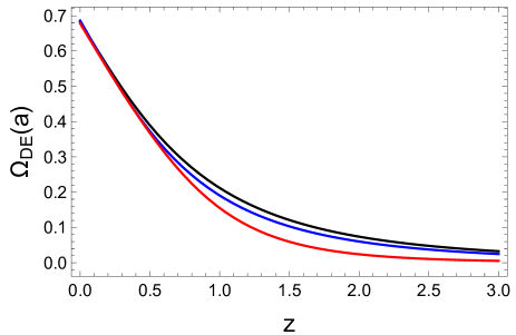
Figure 1: Comparison of the time behaviour of dark energy component, $\Omega_{DE}(a)$ for three different scenarios: black - $\Lambda$CDM; blue - $w=const.$; red - ripped $\Lambda$CDM with $\eta=2.5$. The curves are drawn using the parameter values minimizing the $\chi^{2}$; errors intervals are omitted just for the sake of clarity.

[controls,width=8cm]1gif/prova_113

Figure 2: Dynamical visualization of the equation of state parameter, $w_{(}z)$ sampled from $z=0.$ to $z=3$, with fixed $0.25$ steps.

V Conclusions

Predicting the fate of the Universe may seem philosophy, but it is quite a physical strive. A battery of background astrophysical and cosmological probes may assist us in giving a strong picture of the dynamics of the Universe from close to its very beginning to the current moment. This allows us to put restrictions on the degrees of freedom of a model defined through a specific functional form on its dark energy density. A detailed discussion confirms that our study case, Eq. (2) reproduces a cosmological model with phantom behaviour all throughout its history to reach an asymptotic abrupt end in the form of a pseudorip; that is, the energy density evolves into the $p=-\rho$ condition in infinite time. This transition happens very smoothly, as it is parametrized in the form of a particular sigmoid function (which in some contexts is dubbed as Ridge (activation) function Pinkus (2015)). The characteristics of the model suggests coining a new denomination for it: Ripped $\Lambda$CDM.

For our observation-based tests we choose a sufficiently reliable combination of background data sets with well-known cosmic complementarity.

At first level these tools, through a thorough statistical analysis, let us join the consensus on the evidence of a large scale accelerated expansion driven by a mysterious power. But at the next level they reveal some substantial preference (established in terms of rigorous statistical tools like Evidence and the Bayes Factor) for models with a pseudorip finale over $\Lambda$CDM (the so-called concordance model).

Specific and observationally favoured choices of the value of the parameter $\eta$ (such as for instance $\eta=2.5$) may be then considered as interesting one-parameter (free $\lambda$) evolutionary parametrizations of the dark energy to be tested in further depth. This would certainly contribute to strengthening our knowledge about how seriously we can take the possibility of an abrupt destiny of our universe.

References

- Huterer and Shafer (2018) D. Huterer and D. L. Shafer, Rept. Prog. Phys. 81, 016901 (2018), arXiv:1709.01091 [astro-ph.CO] .
- Carroll et al. (2003) S. M. Carroll, M. Hoffman, and M. Trodden, Phys. Rev. D 68, 023509 (2003), arXiv:astro-ph/0301273 .
- Escamilla et al. (2023) L. A. Escamilla, W. Giarè, E. Di Valentino, R. C. Nunes, and S. Vagnozzi, (2023), arXiv:2307.14802 [astro-ph.CO] .
- Vagnozzi (2020) S. Vagnozzi, Phys. Rev. D 102, 023518 (2020), arXiv:1907.07569 [astro-ph.CO] .
- Caldwell et al. (2003) R. R. Caldwell, M. Kamionkowski, and N. N. Weinberg, Phys. Rev. Lett. 91, 071301 (2003), arXiv:astro-ph/0302506 .
- Fernández-Jambrina (2014) L. Fernández-Jambrina, Phys. Rev. D 90, 064014 (2014).
- Fernández-Jambrina (2016) L. Fernández-Jambrina, Phys. Rev. D 94, 024049 (2016).
- Barrow (2004) J. D. Barrow, Class. Quant. Grav. 21, L79 (2004), arXiv:gr-qc/0403084 .
- Nojiri et al. (2005) S. Nojiri, S. D. Odintsov, and S. Tsujikawa, Phys. Rev. D 71, 063004 (2005), arXiv:hep-th/0501025 .
- Fernández-Jambrina and Lazkoz (2022) L. Fernández-Jambrina and R. Lazkoz, Philosophical Transactions of the Royal Society A: Mathematical, Physical and Engineering Sciences 380, 20210333 (2022).
- Barvinsky et al. (2008) A. O. Barvinsky, C. Deffayet, and A. Y. Kamenshchik, JCAP 05, 020 (2008), arXiv:0801.2063 [hep-th] .
- Bouhmadi-Lopez et al. (2008) M. Bouhmadi-Lopez, P. F. Gonzalez-Diaz, and P. Martin-Moruno, Int. J. Mod. Phys. D 17, 2269 (2008), arXiv:0707.2390 [gr-qc] .
- Dabrowski and Denkiewicz (2009) M. P. Dabrowski and T. Denkiewicz, Phys. Rev. D 79, 063521 (2009).
- Fernández-Jambrina (2010) L. Fernández-Jambrina, Phys. Rev. D 82, 124004 (2010).
- Fernández-Jambrina (2007) L. Fernández-Jambrina, Physics Letters B 656, 9 (2007).
- Frampton et al. (2011) P. H. Frampton, K. J. Ludwick, and R. J. Scherrer, Phys. Rev. D 84, 063003 (2011).
- Frampton et al. (2012a) P. H. Frampton, K. J. Ludwick, S. Nojiri, S. D. Odintsov, and R. J. Scherrer, Physics Letters B 708, 204 (2012a).
- Bouhmadi-Lopez et al. (2015) M. Bouhmadi-Lopez, A. Errahmani, P. Martin-Moruno, T. Ouali, and Y. Tavakoli, Int. J. Mod. Phys. D 24, 1550078 (2015), arXiv:1407.2446 [gr-qc] .
- Frampton et al. (2012b) P. H. Frampton, K. J. Ludwick, and R. J. Scherrer, Phys. Rev. D 85, 083001 (2012b).
- Seikel et al. (2012) M. Seikel, C. Clarkson, and M. Smith, JCAP 06, 036 (2012), arXiv:1204.2832 [astro-ph.CO] .
- Holsclaw et al. (2010a) T. Holsclaw, U. Alam, B. Sanso, H. Lee, K. Heitmann, S. Habib, and D. Higdon, Phys. Rev. D 82, 103502 (2010a), arXiv:1009.5443 [astro-ph.CO] .
- Holsclaw et al. (2010b) T. Holsclaw, U. Alam, B. Sanso, H. Lee, K. Heitmann, S. Habib, and D. Higdon, Phys. Rev. Lett. 105, 241302 (2010b), arXiv:1011.3079 [astro-ph.CO] .
- Holsclaw et al. (2011) T. Holsclaw, U. Alam, B. Sanso, H. Lee, K. Heitmann, S. Habib, and D. Higdon, Phys. Rev. D 84, 083501 (2011), arXiv:1104.2041 [astro-ph.CO] .
- Shafieloo et al. (2012) A. Shafieloo, A. G. Kim, and E. V. Linder, Phys. Rev. D 85, 123530 (2012), arXiv:1204.2272 [astro-ph.CO] .
- Liao et al. (2019) K. Liao, A. Shafieloo, R. E. Keeley, and E. V. Linder, Astrophys. J. Lett. 886, L23 (2019), arXiv:1908.04967 [astro-ph.CO] .
- Keeley et al. (2021) R. E. Keeley, A. Shafieloo, G.-B. Zhao, J. A. Vazquez, and H. Koo, Astron. J. 161, 151 (2021), arXiv:2010.03234 [astro-ph.CO] .
- Hwang et al. (2023) S.-g. Hwang, B. L’Huillier, R. E. Keeley, M. J. Jee, and A. Shafieloo, JCAP 02, 014 (2023), arXiv:2206.15081 [astro-ph.CO] .
- Crittenden et al. (2009) R. G. Crittenden, L. Pogosian, and G.-B. Zhao, JCAP 12, 025 (2009), arXiv:astro-ph/0510293 .
- Huterer and Starkman (2003) D. Huterer and G. Starkman, Phys. Rev. Lett. 90, 031301 (2003), arXiv:astro-ph/0207517 .
- Ruiz et al. (2012) E. J. Ruiz, D. L. Shafer, D. Huterer, and A. Conley, Physical Review D 86 (2012), 10.1103/physrevd.86.103004.
- Daly and Djorgovski (2003) R. A. Daly and S. G. Djorgovski, Astrophys. J. 597, 9 (2003), arXiv:astro-ph/0305197 .
- Daly et al. (2008) R. A. Daly, S. G. Djorgovski, K. A. Freeman, M. P. Mory, C. P. O’Dea, P. Kharb, and S. Baum, Astrophys. J. 677, 1 (2008), arXiv:0710.5345 [astro-ph] .
- Daly and Djorgovski (2007) R. A. Daly and S. G. Djorgovski, Nucl. Phys. B Proc. Suppl. 173, 19 (2007), arXiv:astro-ph/0609791 .
- Daly and Djorgovski (2004) R. A. Daly and S. G. Djorgovski, Astrophys. J. 612, 652 (2004), arXiv:astro-ph/0403664 .
- Abdalla et al. (2022) E. Abdalla et al., JHEAp 34, 49 (2022), arXiv:2203.06142 [astro-ph.CO] .
- Montiel et al. (2014) A. Montiel, R. Lazkoz, I. Sendra, C. Escamilla-Rivera, and V. Salzano, Phys. Rev. D 89, 043007 (2014), arXiv:1401.4188 [astro-ph.CO] .
- Rana et al. (2016) A. Rana, D. Jain, S. Mahajan, and A. Mukherjee, JCAP 07, 026 (2016), arXiv:1511.09223 [astro-ph.CO] .
- Turner and White (1997) M. S. Turner and M. J. White, Phys. Rev. D 56, R4439 (1997), arXiv:astro-ph/9701138 .
- Saini et al. (2000) T. D. Saini, S. Raychaudhury, V. Sahni, and A. A. Starobinsky, Phys. Rev. Lett. 85, 1162 (2000), arXiv:astro-ph/9910231 .
- Capozziello et al. (2011) S. Capozziello, R. Lazkoz, and V. Salzano, Phys. Rev. D 84, 124061 (2011), arXiv:1104.3096 [astro-ph.CO] .
- Visser (2005) M. Visser, Gen. Rel. Grav. 37, 1541 (2005), arXiv:gr-qc/0411131 .
- Cattoen and Visser (2008) C. Cattoen and M. Visser, Phys. Rev. D 78, 063501 (2008), arXiv:0809.0537 [gr-qc] .
- Guimaraes and Lima (2011) A. C. C. Guimaraes and J. A. S. Lima, Class. Quant. Grav. 28, 125026 (2011), arXiv:1005.2986 [astro-ph.CO] .
- Cai and Tuo (2011) R.-G. Cai and Z.-L. Tuo, Phys. Lett. B 706, 116 (2011), arXiv:1105.1603 [astro-ph.CO] .
- Aviles et al. (2012) A. Aviles, C. Gruber, O. Luongo, and H. Quevedo, Phys. Rev. D 86, 123516 (2012), arXiv:1204.2007 [astro-ph.CO] .
- Zaninetti (2016) L. Zaninetti, Galaxies 4, 4 (2016), arXiv:1602.06418 [astro-ph.CO] .
- Gruber and Luongo (2014) C. Gruber and O. Luongo, Phys. Rev. D 89, 103506 (2014), arXiv:1309.3215 [gr-qc] .
- Shchigolev (2017) V. K. Shchigolev, Grav. Cosmol. 23, 142 (2017), arXiv:1511.07459 [gr-qc] .
- Yu et al. (2021) B. Yu, J.-C. Zhang, T.-J. Zhang, and T. Zhang, Phys. Dark Univ. 31, 100772 (2021), arXiv:2101.05276 [astro-ph.CO] .
- Bargiacchi et al. (2021) G. Bargiacchi, G. Risaliti, M. Benetti, S. Capozziello, E. Lusso, A. Saccardi, and M. Signorini, Astron. Astrophys. 649, A65 (2021), arXiv:2101.08278 [astro-ph.CO] .
- Colgáin et al. (2021) E. O. Colgáin, M. M. Sheikh-Jabbari, and L. Yin, Phys. Rev. D 104, 023510 (2021), arXiv:2104.01930 [astro-ph.CO] .
- Wetterich (2004) C. Wetterich, Phys. Lett. B 594, 17 (2004), arXiv:astro-ph/0403289 .
- Jassal et al. (2005) H. K. Jassal, J. S. Bagla, and T. Padmanabhan, Mon. Not. Roy. Astron. Soc. 356, L11 (2005), arXiv:astro-ph/0404378 .
- Feng et al. (2012) C.-J. Feng, X.-Y. Shen, P. Li, and X.-Z. Li, JCAP 09, 023 (2012), arXiv:1206.0063 [astro-ph.CO] .
- Nesseris and Perivolaropoulos (2004) S. Nesseris and L. Perivolaropoulos, Phys. Rev. D 70, 043531 (2004), arXiv:astro-ph/0401556 .
- Linder (2006) E. V. Linder, Phys. Rev. D 73, 063010 (2006), arXiv:astro-ph/0601052 .
- Cooray and Huterer (1999) A. R. Cooray and D. Huterer, Astrophys. J. Lett. 513, L95 (1999), arXiv:astro-ph/9901097 .
- Ma and Zhang (2011) J.-Z. Ma and X. Zhang, Phys. Lett. B 699, 233 (2011), arXiv:1102.2671 [astro-ph.CO] .
- Mukherjee and Banerjee (2016) A. Mukherjee and N. Banerjee, Phys. Rev. D 93, 043002 (2016), arXiv:1601.05172 [gr-qc] .
- Gong and Zhang (2005) Y.-g. Gong and Y.-Z. Zhang, Phys. Rev. D 72, 043518 (2005), arXiv:astro-ph/0502262 .
- Lee (2005) S. Lee, Phys. Rev. D 71, 123528 (2005), arXiv:astro-ph/0504650 .
- Upadhye et al. (2005) A. Upadhye, M. Ishak, and P. J. Steinhardt, Phys. Rev. D 72, 063501 (2005), arXiv:astro-ph/0411803 .
- Gerke and Efstathiou (2002) B. F. Gerke and G. Efstathiou, Mon. Not. Roy. Astron. Soc. 335, 33 (2002), arXiv:astro-ph/0201336 .
- Lazkoz et al. (2011) R. Lazkoz, V. Salzano, and I. Sendra, Phys. Lett. B 694, 198 (2011), arXiv:1003.6084 [astro-ph.CO] .
- Sendra and Lazkoz (2012) I. Sendra and R. Lazkoz, Mon. Not. Roy. Astron. Soc. 422, 776 (2012), arXiv:1105.4943 [astro-ph.CO] .
- Feng and Lu (2011) L. Feng and T. Lu, Journal of Cosmology and Astroparticle Physics 2011, 034 (2011), arXiv:1203.1784v2 [astro-ph.CO] .
- Efstathiou (1999) G. Efstathiou, Mon. Not. Roy. Astron. Soc. 310, 842 (1999), arXiv:astro-ph/9904356 .
- Barboza and Alcaniz (2012) E. M. Barboza, Jr. and J. S. Alcaniz, JCAP 02, 042 (2012), arXiv:1103.0257 [astro-ph.CO] .
- Yang et al. (2021) W. Yang, E. Di Valentino, S. Pan, A. Shafieloo, and X. Li, Phys. Rev. D 104, 063521 (2021), arXiv:2103.03815 [astro-ph.CO] .
- Fernández-Jambrina and Lazkoz (2009) L. Fernández-Jambrina and R. Lazkoz, Physics Letters B 670, 254 (2009).
- Scolnic et al. (2022) D. Scolnic et al., Astrophys. J. 938, 113 (2022), arXiv:2112.03863 [astro-ph.CO] .
- Peterson et al. (2022) E. R. Peterson et al., Astrophys. J. 938, 112 (2022), arXiv:2110.03487 [astro-ph.CO] .
- Carr et al. (2022) A. Carr, T. M. Davis, D. Scolnic, D. Scolnic, K. Said, D. Brout, E. R. Peterson, and R. Kessler, Publ. Astron. Soc. Austral. 39, e046 (2022), arXiv:2112.01471 [astro-ph.CO] .
- Brout et al. (2022) D. Brout et al., Astrophys. J. 938, 110 (2022), arXiv:2202.04077 [astro-ph.CO] .
- Jimenez and Loeb (2002) R. Jimenez and A. Loeb, Astrophys. J. 573, 37 (2002), arXiv:astro-ph/0106145 .
- Moresco et al. (2011) M. Moresco, R. Jimenez, A. Cimatti, and L. Pozzetti, JCAP 03, 045 (2011), arXiv:1010.0831 [astro-ph.CO] .
- Moresco et al. (2018) M. Moresco, R. Jimenez, L. Verde, L. Pozzetti, A. Cimatti, and A. Citro, Astrophys. J. 868, 84 (2018), arXiv:1804.05864 [astro-ph.CO] .
- Moresco et al. (2020) M. Moresco, R. Jimenez, L. Verde, A. Cimatti, and L. Pozzetti, Astrophys. J. 898, 82 (2020), arXiv:2003.07362 [astro-ph.GA] .
- Moresco et al. (2022) M. Moresco et al., Living Rev. Rel. 25, 6 (2022), arXiv:2201.07241 [astro-ph.CO] .
- Moresco et al. (2012a) M. Moresco, L. Verde, L. Pozzetti, R. Jimenez, and A. Cimatti, JCAP 07, 053 (2012a), arXiv:1201.6658 [astro-ph.CO] .
- Moresco et al. (2012b) M. Moresco et al., JCAP 08, 006 (2012b), arXiv:1201.3609 [astro-ph.CO] .
- Moresco (2015) M. Moresco, Mon. Not. Roy. Astron. Soc. 450, L16 (2015), arXiv:1503.01116 [astro-ph.CO] .
- Moresco et al. (2016) M. Moresco, R. Jimenez, L. Verde, A. Cimatti, L. Pozzetti, C. Maraston, and D. Thomas, JCAP 12, 039 (2016), arXiv:1604.00183 [astro-ph.CO] .
- Moresco and Marulli (2017) M. Moresco and F. Marulli, Mon. Not. Roy. Astron. Soc. 471, L82 (2017), arXiv:1705.07903 [astro-ph.CO] .
- Jimenez et al. (2019) R. Jimenez, A. Cimatti, L. Verde, M. Moresco, and B. Wandelt, JCAP 03, 043 (2019), arXiv:1902.07081 [astro-ph.CO] .
- Jiao et al. (2023) K. Jiao, N. Borghi, M. Moresco, and T.-J. Zhang, Astrophys. J. Suppl. 265, 48 (2023), arXiv:2205.05701 [astro-ph.CO] .
- Liu and Wei (2015) J. Liu and H. Wei, Gen. Rel. Grav. 47, 141 (2015), arXiv:1410.3960 [astro-ph.CO] .
- Conley et al. (2011) A. Conley et al. (SNLS), Astrophys. J. Suppl. 192, 1 (2011), arXiv:1104.1443 [astro-ph.CO] .
- Aghanim et al. (2020) N. Aghanim et al. (Planck), Astron. Astrophys. 641, A6 (2020), [Erratum: Astron.Astrophys. 652, C4 (2021)], arXiv:1807.06209 [astro-ph.CO] .
- Wang and Mukherjee (2007) Y. Wang and P. Mukherjee, Phys. Rev. D 76, 103533 (2007), arXiv:astro-ph/0703780 .
- Zhai et al. (2020) Z. Zhai, C.-G. Park, Y. Wang, and B. Ratra, JCAP 07, 009 (2020), arXiv:1912.04921 [astro-ph.CO] .
- Hu and Sugiyama (1996) W. Hu and N. Sugiyama, Astrophys.J. 471, 542 (1996), arXiv:astro-ph/9510117 .
- Blake et al. (2012) C. Blake et al., Mon. Not. Roy. Astron. Soc. 425, 405 (2012), arXiv:1204.3674 [astro-ph.CO] .
- Tamone et al. (2020) A. Tamone et al., Mon. Not. Roy. Astron. Soc. 499, 5527 (2020), arXiv:2007.09009 [astro-ph.CO] .
- de Mattia et al. (2021) A. de Mattia et al., Mon. Not. Roy. Astron. Soc. 501, 5616 (2021), arXiv:2007.09008 [astro-ph.CO] .
- Alam et al. (2017) S. Alam et al. (BOSS), Mon. Not. Roy. Astron. Soc. 470, 2617 (2017), arXiv:1607.03155 [astro-ph.CO] .
- Gil-Marin et al. (2020) H. Gil-Marin et al., Mon. Not. Roy. Astron. Soc. 498, 2492 (2020), arXiv:2007.08994 [astro-ph.CO] .
- Bautista et al. (2020) J. E. Bautista et al., Mon. Not. Roy. Astron. Soc. 500, 736 (2020), arXiv:2007.08993 [astro-ph.CO] .
- Nadathur et al. (2020) S. Nadathur et al., Mon. Not. Roy. Astron. Soc. 499, 4140 (2020), arXiv:2008.06060 [astro-ph.CO] .
- du Mas des Bourboux et al. (2020) H. du Mas des Bourboux et al., Astrophys. J. 901, 153 (2020), arXiv:2007.08995 [astro-ph.CO] .
- Hou et al. (2020) J. Hou et al., Mon. Not. Roy. Astron. Soc. 500, 1201 (2020), arXiv:2007.08998 [astro-ph.CO] .
- Neveux et al. (2020) R. Neveux et al., Mon. Not. Roy. Astron. Soc. 499, 210 (2020), arXiv:2007.08999 [astro-ph.CO] .
- Eisenstein and Hu (1998) D. J. Eisenstein and W. Hu, Astrophys. J. 496, 605 (1998), arXiv:astro-ph/9709112 [astro-ph] .
- Zhao et al. (2019) G.-B. Zhao et al., Mon. Not. Roy. Astron. Soc. 482, 3497 (2019), arXiv:1801.03043 [astro-ph.CO] .
- Dunkley et al. (2005) J. Dunkley, M. Bucher, P. G. Ferreira, K. Moodley, and C. Skordis, Mon. Not. Roy. Astron. Soc. 356, 925 (2005), arXiv:astro-ph/0405462 .
- Kass and Raftery (1995) R. E. Kass and A. E. Raftery, Journal of the American Statistical Association 90, 773 (1995).
- Mukherjee et al. (2006) P. Mukherjee, D. Parkinson, and A. R. Liddle, Astrophys. J. Lett. 638, L51 (2006), arXiv:astro-ph/0508461 .
- Jeffreys (1939) H. Jeffreys, Theory of Probability (Oxford, England: Clarendon Press, 1939).
- Pinkus (2015) A. Pinkus, “Introduction,” in Ridge Functions, Cambridge Tracts in Mathematics (Cambridge University Press, 2015) p. 1–11.