Mind the map! Accounting for existing map information
when estimating online HDMaps from sensor data

Abstract

Online High Definition Map (HDMap) estimation from sensors offers a low-cost alternative to manually acquired HDMaps. As such, it promises to lighten costs for already HDMap-reliant Autonomous Driving systems, and potentially even spread their use to new systems.

In this paper, we propose to improve online HDMap estimation by accounting for already existing maps. We identify 3 reasonable types of useful existing maps (minimalist, noisy, and outdated). We also introduce MapEX, a novel online HDMap estimation framework that accounts for existing maps. MapEX achieves this by encoding map elements into query tokens and by refining the matching algorithm used to train classic query based map estimation models.

We demonstrate that MapEX brings significant improvements on the nuScenes dataset. For instance, MapEX - given noisy maps - improves by 38% over the MapTRv2 detector it is based on and by 16% over the current SOTA.

1 Introduction

Autonomous Driving [24, 12] represents a complex problem that promises to significantly change how we interact with transportation. While full vehicle automation still seems quite a ways away [41], partially autonomous vehicles now populate a number of road systems in the world [24]. These vehicles need to process a wealth of information to function, from the raw sensor data [15] to elaborate maps of road networks [12, 28].

High Definition maps (HDMaps), in particular, represent a crucial component of the research on self-driving cars [12, 11] (see Fig. 1 for a few simple examples of maps, with road boundaries represented by green polylines, lane dividers by lime polylines and pedestrian crossings by blue polygons). Although maps are not a typical input of neural networks, they contain necessary information to help the car understand the world it must navigate. As such, significant efforts have gone into incorporating this new type of data into proposed solutions [12, 37]. These efforts have in turn shown HDMaps have remarkable benefits both for fundamental problems like Object Detection [18] to precise trajectory forecasting problems [28, 37].

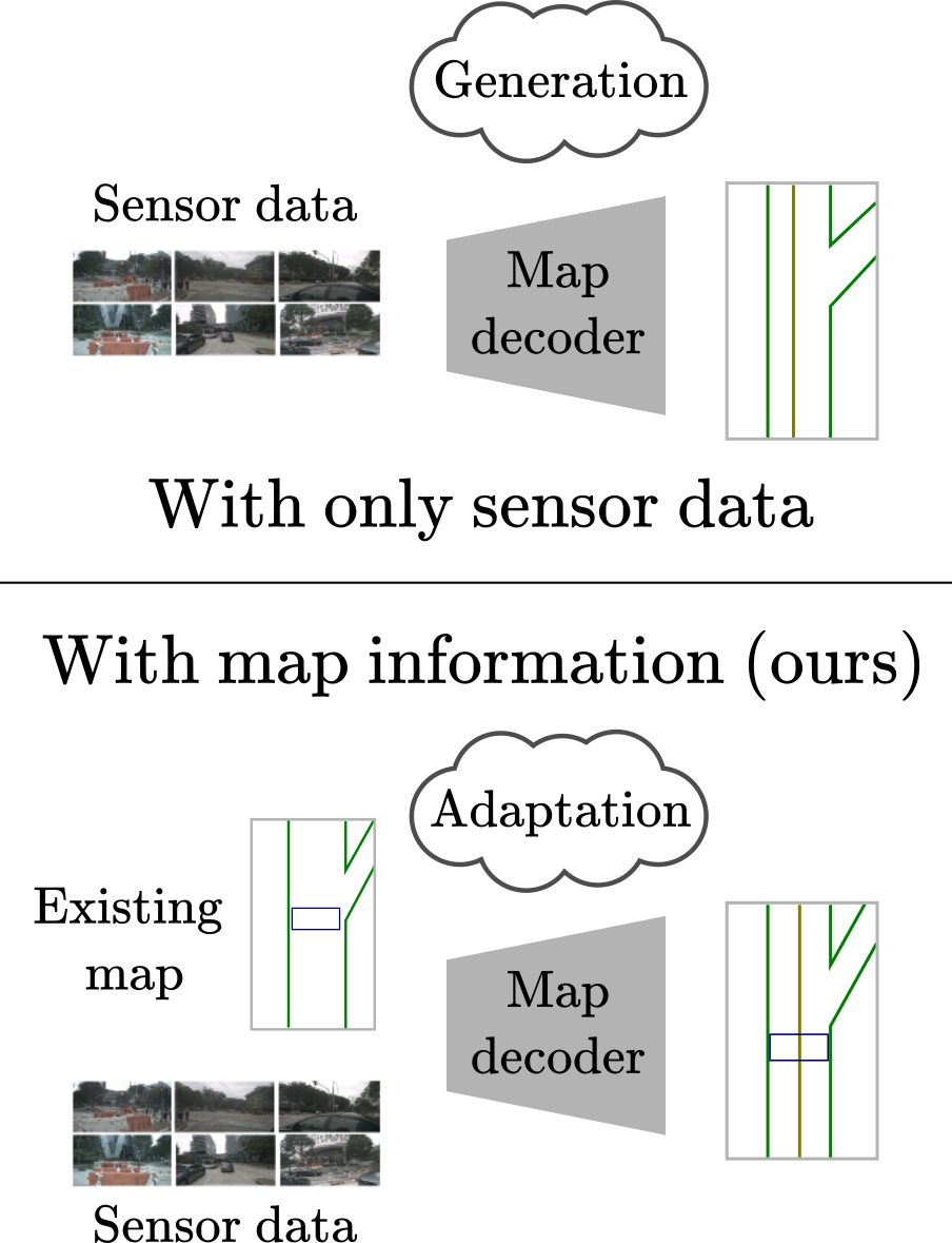
Figure 1: We propose to use existing map information - even if inexact - to estimate better online HDMaps from sensor inputs. In doing so, we simplify the problem from generating maps using only sensors to re-using always available maps aided by sensors.

These maps are however expensive to acquire and maintain, requiring precise data acquisition and exacting human labeling efforts [11, 21]. There has therefore been a strong push over the last year [5, 29] to approximate online HDMaps from sensor data. It is interesting to note that even seminal work on the subject has produced useful maps for trajectory forecasting [33].

While recent methods like MapTRv2 [30] have become proficient at generating online HDMaps from raw sensors, we feel they overlook very useful and nearly always available data: existing maps. We posit here that outdated or lower quality maps should usually be available and could significantly improve the acquired HDMaps as illustrated in Fig. 1. Indeed, even “map-free” models tend to use lower-quality satnav maps [1], and estimated maps could always be available as long as a vehicle went through a place once.

In this paper, we explore the central postulate that inaccurate maps can be used to improve the estimation of HDMaps from raw sensors as shown on Fig. 1. After providing some context on our method and the field in Sec. 2, we propose two distinct technical contributions. In Sec. 3, we outline reasonable scenarios under which an inaccurate map can be available along with practical implementations. In Sec. 4, we propose MapEX, an architecture that can generate HDMaps from sensor data while accounting for existing map information. Finally, we present results in Sec. 5 with experiments on the nuScenes dataset [4].
Contributions We offer the following 3 contributions:

• We propose to account for existing Map information when estimating online HDMaps from sensor data.

• We discuss reasonable scenarios under which existing maps are not perfect. We also provide realistic implementations of these scenarios and code for the nuScenes dataset.

• We introduce MapEX, a new query based HDMap acquisition scheme that can incorporate map information when estimating an online HDMap from sensors. In particular, we introduce with MapEX both a novel way to incorporate existing map information with existing (EX) queries and a way to help the model learn to leverage this information by pre-attributing predictions to ground truths during training.

We demonstrate experimentally that our contribution lead to substantial improvements in online HDMap acquisition from sensors on the nuScenes dataset. In the scenario where we use HDMaps with noisy (or “shifted”) map element positions for instance, MapEX reaches a 84.8% mAP score which is an improvement of 38% over the MapTRv2 detector it is based on and a 16% improvement over the current state-of-the-art as shown in Tab. 1.

Method	Backbone	Epochs	Extra info	mAP
MapTRv2 (Base)	R50	24	✗	61.5
MapTRv2 (SOTA)	V2-99	110	Depth pretraining	73.4
MapEX-S2a (Ours)	R50	24	Inaccurate map	84.8

Table 1: MapEX strongly improves on existing online HDMap estimation methods and beats the current state-of-the-art mean average precision (mAP) by 16% in the median scenario on nuScenes.

2 Related Work

We provide here some brief context on HDMaps in autonomous driving. We begin by discussing HDMap’s use in trajectory forecasting, before discussing their acquisition. We then discuss online HDMap estimation itself.
HDMaps for trajectory forecasting Autonomous Driving often requires a lot of information about the world vehicles are to navigate. This information is typically embedded in rich HDMaps given as input to modified neural networks [16, 37]. HDMaps have proven critical to the performance of a number of modern methods in trajectory forecasting [37, 9] and other applications [18]. In trajectory forecasting in particular, it is remarkable that some methods [32, 31] explicitly reason on a representation of the HDMap and therefore absolutely require access to a HDMap [40]. [33] reports a 10% drop in performance for a common forecasting technique [32] when applied without an informative HDMap. [44] reports even more dramatic drops in performance for other well known methods.
HDMap acquisition and maintenance Unfortunately, HDMaps are expensive to acquire and maintain [11, 21]. While HDMaps used in forecasting are only a simplified version containing map elements (lane dividers, road boundaries, …) [26, 30] and foregoing much of the complex information in full HDMaps [11], they still require exceedingly precise measurements (on the scale of tens of centimeters) [11]. A number of companies have therefore been moving towards a less exacting Medium Definition Maps (MDMaps) standard [17], or even towards satellite navigation maps (Google Maps, SDMaps) [1]. Crucially, MDMaps - with their precision of a few meters - would be a good example of an existing map giving valuable information for the online HDMap generation process. Our map Scenario 2a explores an approximation of this situation.
Online HDMap estimation from sensors Online HDMap estimation [5] has therefore emerged as a promising alternative to manually curated HDMaps. While some works [5, 45, 6] focus on predicting virtual map elements, i.e. lane centerlines, the standard formulation introduced by [26] focuses on more visually recognizable map elements: lane dividers, road boundaries and pedestrian crossings. Probably because visual elements are easier to detect by sensors, this latter formulation has seen rapid progress over the last year [33, 29, 10]. Interestingly, the latest such method - MapTRv2 [30] - does offer an auxiliary setting for detecting virtual lane centerlines. This suggests a natural convergence towards the more complex settings comprising a multitude of additional map elements (traffic lights, …) [27, 42]. Nevertheless, the standard formulation from [26] remains the gold standard when evaluating the usefulness of additional information such as learned global feature maps [43], satellite views [13], or SDMaps [2]. We thus keep to this problem formulation to demonstrate the use of existing map information.

Our work is adjacent to the commonly studied change detection problems [34, 3] that aim to detect a change in a map (e.g. crossings). While rooted in more classical statistical techniques [34], a few efforts have been made to adapt them to deep learning [20, 3]. Notably, the Argoverse 2 Trust but Verify (TbV) dataset [25] was recently proposed for this problem (see Appendix 8). This however differs substantially from our approach as we do not try to correct small mistakes on an existing map after aggregating from a fleet of vehicles [35, 22]. Instead we aim to generate accurate online HDMaps with the help of an existing - possibly very different - map, which is made possible by the modern online HDMap estimation problem. Therefore, we do not only correct small mistakes in maps but propose a more expressive framework that accommodates any change (e.g. distorted lines, very noisy elements).

3 What kind of existing map could we use?

We make the central claim that accounting for existing maps would benefit online HDMaps estimation. We argue here there are many reasonable scenarios under which imperfect maps can appear. After defining the HDMap representations we work with in Sec. 3.1 and our general approach in Sec. 3.2, we consider three main possibilities: only road boundaries are available (Sec. 3.3), the maps are noisy (Sec. 3.4), or they have changed substantially (Sec. 3.5).

3.1 HDMap representation for online HDMap estimation from sensors

We adopt the standard format used for online HDMaps generation from sensors [26, 29]: we consider HDMaps to be made of 3 types of polylines, road boundaries, lane dividers and pedestrian crosswalks, with same colors as previously green, lime, and blue respectively, as represented on Fig. 2(a). We follow [29] by representing these polylines as sets of 20 evenly spaced points for our map generator, and using upsampled versions for evaluation.

While true HDMaps are much more complex [11] and more intricate representations have been proposed [6], the aim of this work is to study how to account for existing map information. As such we restrict ourselves to the most commonly studied formulation. The work in this paper will be directly applicable to the prediction of more map elements [6], finer polylines [10, 39] or rasterized objectives [46].

3.2 MapModEX: Simulating imperfect maps

As acquiring genuine imprecise maps for standard map acquisition datasets (e.g. nuScenes) would be costly and time consuming, we synthetically generate imprecise maps from existing HDMaps.

We develop MapModEX, a standalone map modification library. It takes nuScenes map files and sample records, and for each sample outputs polyline coordinates for dividers, boundaries and pedestrian crosswalks in a given patch, around the ego vehicle. Importantly, our library provides the ability to modify these polylines to reflect various modifications: removal of map elements, addition, shifting of pedestrian crossings, noise addition to point coordinates, map shift, map rotation and map warping. MapModEX will be made available after publication to facilitate further research into incorporating existing maps into online HDMap acquisition from sensors.

We implement three challenging scenarios, outlined next, using our MapModEX package, generating for each sample 10 variants of scenarios 2 and 3 (scenario 1 only admits one variant). We chose to work with a fixed set of modified maps to reduce online computation costs during training and to reflect real situations where only a finite number of map variants might be available.

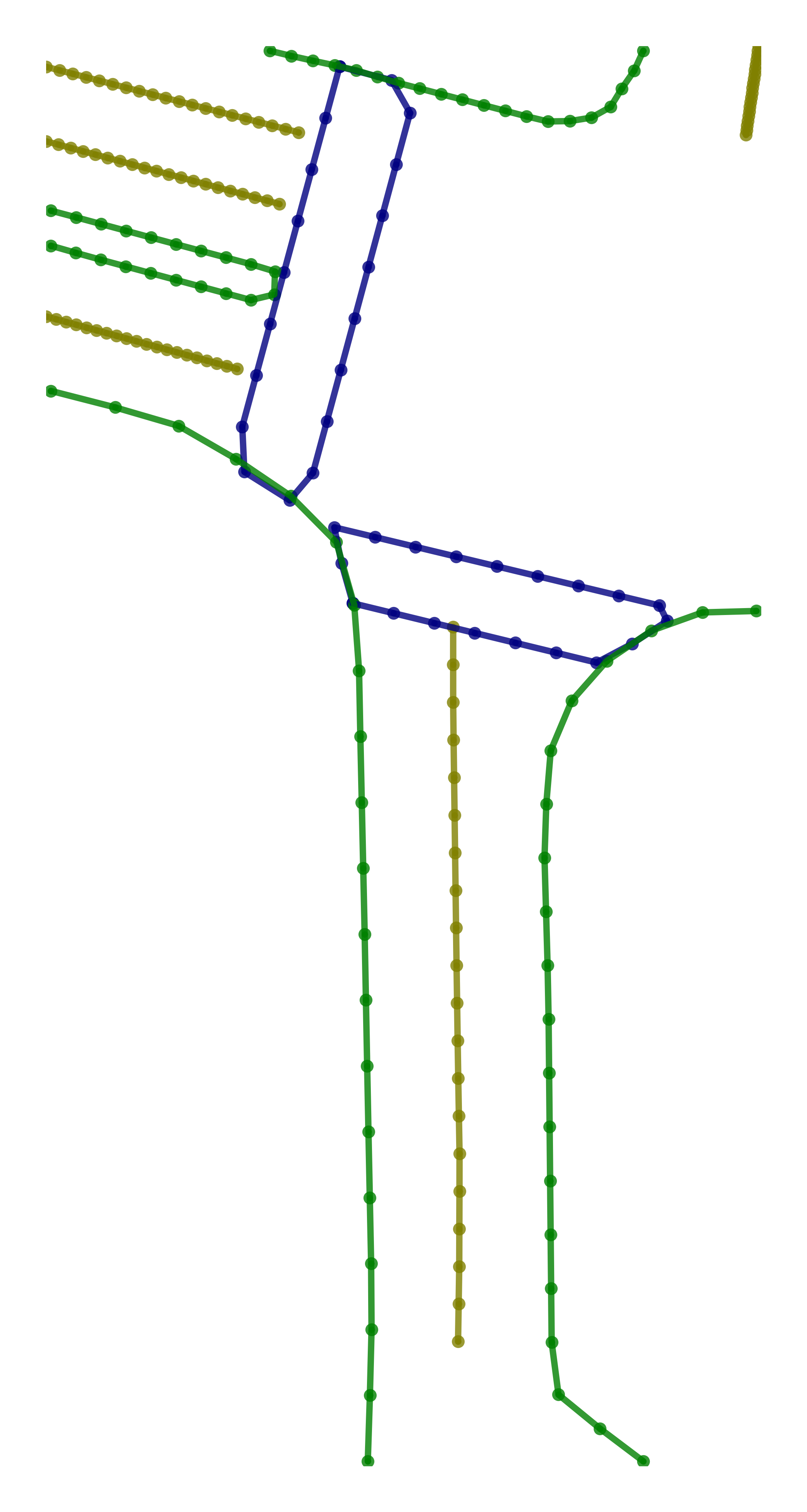
(a) Ground Truth.

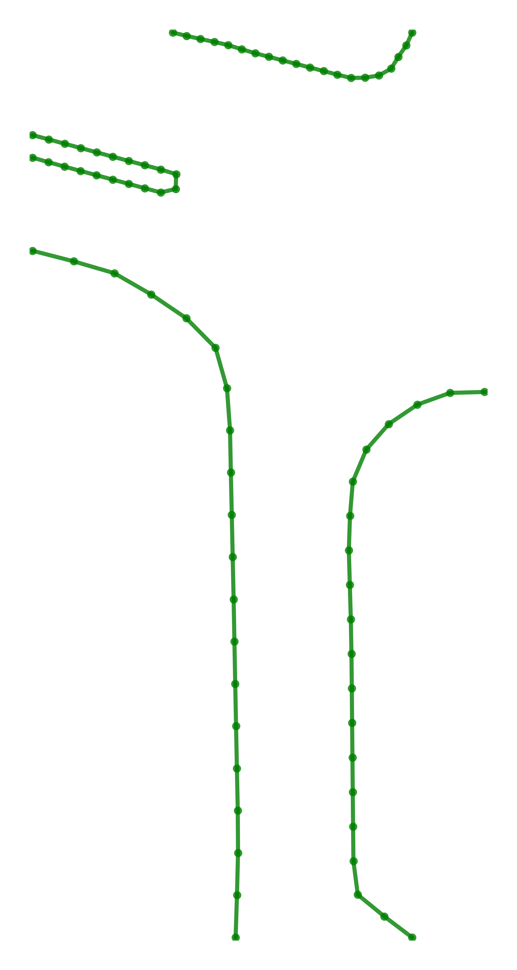
(b) Scenario 1.

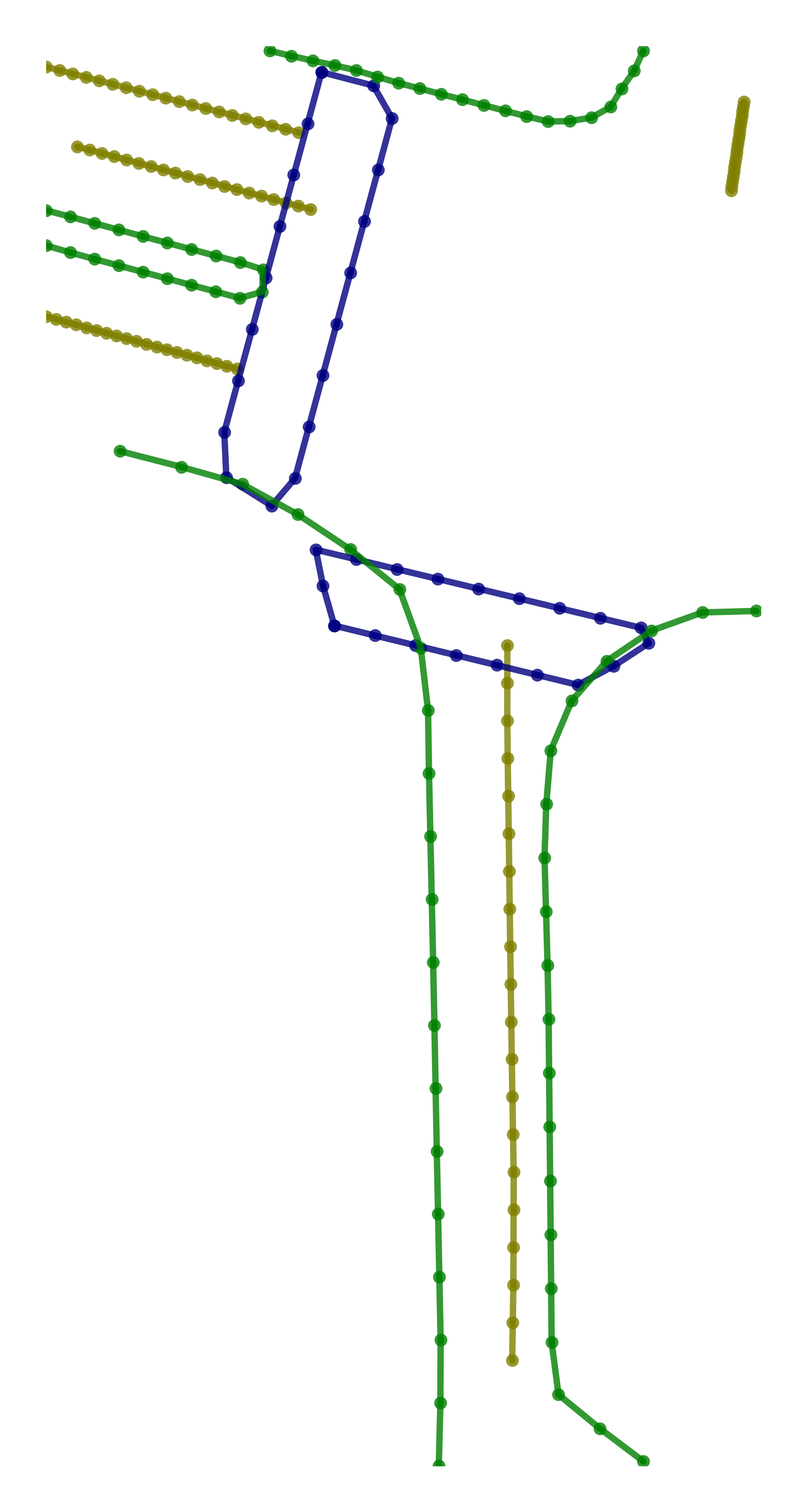
(c) Scenario 2a.

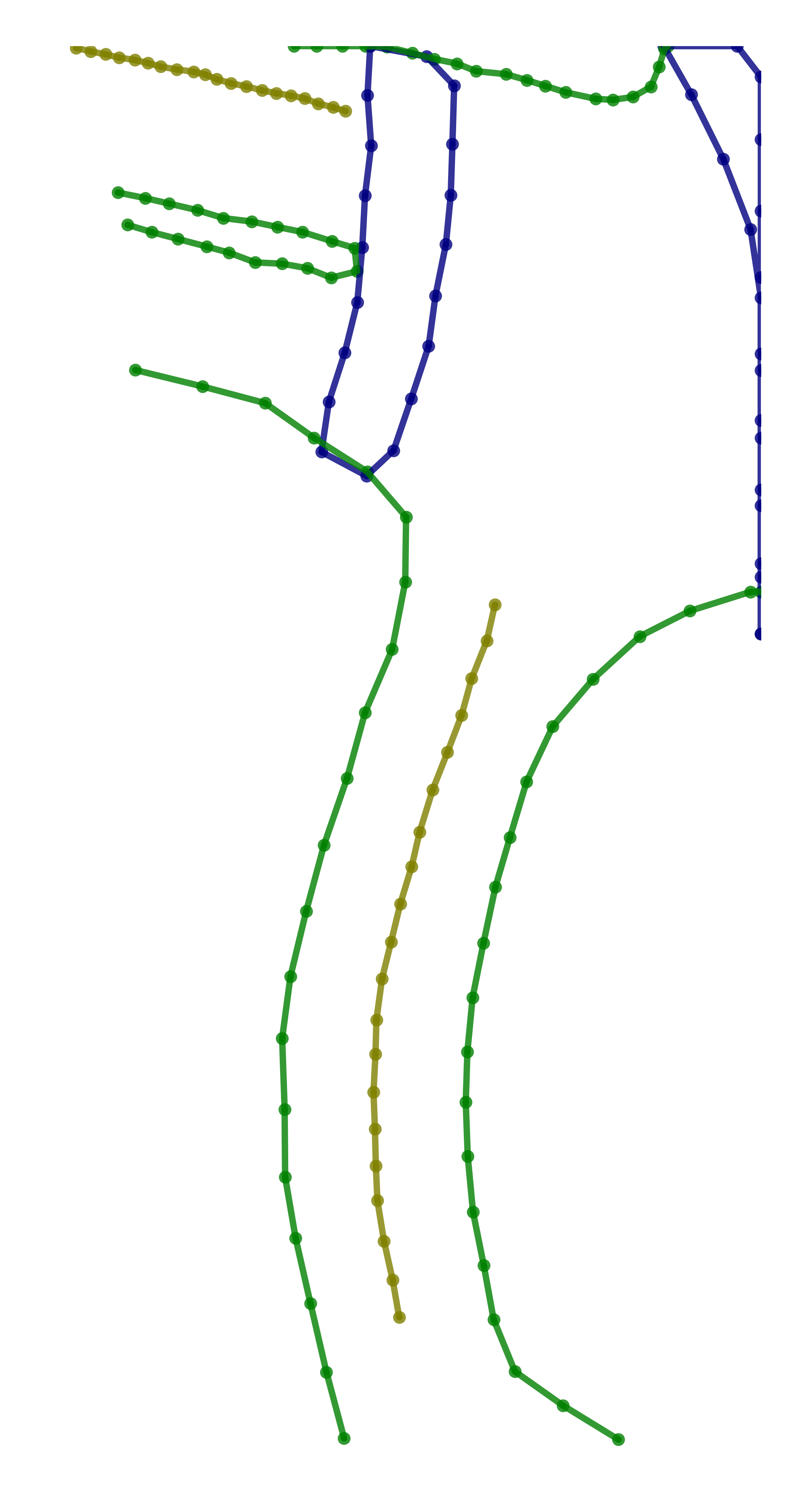
(d) Scenario 3a.

Figure 2: Examples of HDMaps generated by MapModEX.

3.3 Scenario 1: Only boundaries are available

A first scenario is one where only a bare HDMap (without divider and pedestrian crossings) is available as shown on Fig. 2(b). Road boundaries are more often associated with 3D physical landmarks (e.g. edge of sidewalk) whereas dividers and pedestrian crossings are generally denoted by flat painted markings that are easier to miss. Moreover, pedestrian crossings and lane dividers are fairly commonly displaced by construction works or road deviations, or even partially hidden by tire tracks.

As such, it is reasonable to use HDMaps with only boundaries. This would have the benefit of reducing annotators costs by only asking annotators to label road boundaries. Furthermore, less precise equipment and less updates might be required to situate only road boundaries.
Implementation From a practical standpoint, Scenario 1 implementation is straightforward: we remove the divider and pedestrian crossings from available HDMaps.

3.4 Scenario 2: Maps are noisy

A second plausible case is one where we only have very noisy maps as shown on Fig. 2(c). A weak point of existing HDMaps is the need for high precision (in the order of a few centimeters), which puts a significant strain on their acquisition and maintenance [11]. In fact, a key difference between HDMaps and the emergent MDMaps standard lies in a lower precision (a few centimeters vs. a few meters).

We therefore propose to work with noisy HDMaps to simulate situations where less precise maps could be the result of a cheaper acquisition process or a move to the MDMaps standard. More interestingly, these less precise maps could be automatically obtained from sensor data. Although methods like MapTRv2 have reached very impressive performance, they are not yet completely precise: even with very flexible retrieval thresholds, the precision of predictions falls far short of 80%.
Implementation We propose two possible implementations of these noisy HDMaps to reflect the various conditions under which we might be lacking precision. In a first Scenario 2a, we propose a shift-noise setting where for each map element localization, we add noise from a Gaussian distribution with standard deviation of 1 meter. This has the effect of applying a uniform translation to each map element (dividers, boundaries, crosswalks). Such a setting should be a good approximation of situations where human annotators provide quick imprecise annotations from noisy data. We chose a standard deviation of 1 meter to reflect MDMaps standards of being precise up to a few meters [17].

We then test our approach with a very challenging pointwise-noise Scenario 2b: for each ground truth point - keeping in mind a map element is made up of 20 such points - we sample noise from a Gaussian distribution with standard deviation of 5 meters and add it to the point coordinates. This provides a worst case approximation of the situation where the map was acquired automatically or provides very imprecise localization.

3.5 Scenario 3: Maps have substantially changed

The final scenario we consider is one where we have access to old maps that used to be accurate (see Fig. 2(d)). As noted in Sec. 3.3, it is fairly common for painted markers like pedestrian crossings to be displaced from time to time. Furthermore, it is not uncommon for cities to substantially remodel some problematic intersection or renovate districts to accommodate traffic increase by a new attraction [38].

It is therefore interesting to use HDMaps that are valid on their own but differ from the actual HDMaps in significant ways. These maps should often appear when the HDMaps are only updated by the maintainer every few years to cut down on costs. In that case, the available maps would still provide some information on the world but might not reflect temporary or recent changes.
Implementation We approximate this by applying strong changes to existing HDMaps in our Scenario 3a. We delete 50% of the pedestrian crossings and lane dividers in the map, add a few pedestrian crossings (half the amount of the remaining crossings) and finally apply a small warping distortion to the map.

However, it is important to note that a substantial amount of the global map will remain unchanged over time. We account for that in our Scenario 3b, where we study the effect of randomly choosing (with probability p=0.5) to consider the real HDMap instead of the perturbed version.

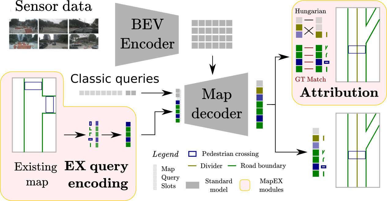
Figure 3: Overview of our MapEX method (see Sec. 4). We add two modules (EX query encoding, Attribution) to the standard query based map estimation pipeline (in gray on the figure). Map elements are encoded into EX queries, then decoded with a standard decoder.

4 MapEX: Accounting for EXisting maps

We propose MapEX (see Fig. 3), a novel framework for online HDMap estimation. It follows the standard query based online HDMap estimation workflow [33, 29] and processes existing map information thanks to two key modules: a map query encoding module (see Sec. 4.2) and a pre-attribution scheme of predictions and ground truths for training (see Sec. 4.3). We also propose an optional change detection module in Appendix 9 for cases where true maps are mixed with perturbed maps as in our Scenario 3b. Since our implementation is built upon the state-of-the-art MapTRv2 [30], it will translate to most methods [33, 10, 29]

4.1 Overview

The core of the standard query based framework is shown through gray elements on Fig. 3. It starts by taking sensor inputs (cameras and/or LiDAR), and encodes them into a Bird’s Eye View (BEV) representation to serve as sensor features. The map itself is obtained using a DETR-like [7] detection scheme to detect the map elements ($N$ at most). This is achieved by passing $N\times L$ learned query tokens ($N$ being the maximum number of detected elements, $L$ the number of points predicted for an element) into a transformer decoder that feeds sensor information to the query tokens using cross-attention with the BEV features. The decoded queries are then translated into map element coordinates by linear layers along with a class prediction (including an extra background class) such that groups of $L$ queries represent the $L$ points of a map element ($L=20$ in this paper). Training is done by matching predicted map elements and ground truth map elements using some variant of the Hungarian algorithm [23, 8]. Once matched, the model is optimized to fit the predicted map elements to their corresponding ground truth using regression (for coordinates) and classification (for element classes) losses.

This standard framework has no way to account for existing maps, which necessitates introducing new modules at two key levels. At the query level, we encode map elements into non learnable EX queries (see Sec. 4.2). At the matching level, we pre-attribute queries to the ground truth map elements they represent (see Sec. 4.3).

The complete MapEX framework - shown on Fig. 3 - converts existing map elements into non-learnable map queries and adds learnable queries to reach a set number of queries $N\times L$. This completed set of queries is then passed to a transformer decoder and translated into predictions by linear layers as usual. At training time, our attribution module pre-matches a number of predictions with ground truths, and the rest is matched normally using Hungarian Matching. At test time, the decoded non background queries yield a HDMap representation.

4.2 Translating maps into EX queries

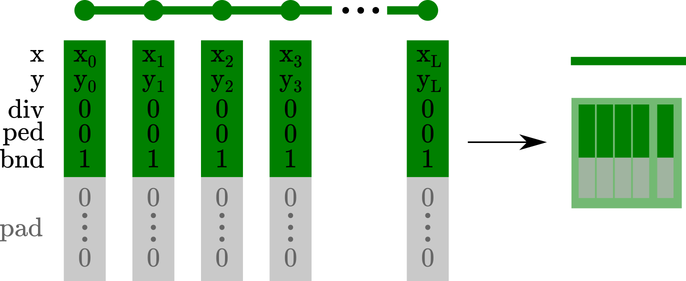
Figure 4: Encoding map elements into EX queries. For each point of the element, we encode the (x,y) coordinates along with the element class. (div=divider, ped=crossing, bnd=boundary)

There is no mechanism in current online HDMap estimation frameworks to account for existing map information. We therefore need to design a new scheme that can translate existing maps into a form understandable by standard query-based online HDMap estimation frameworks. We propose with MapEX a simple method of encoding existing map elements into EX queries for the decoder as shown on Fig. 4.

For a given map element, we extract $L$ evenly spaced points, with $L$ being the number of points we seek to predict for any map element. For each point, we craft an EX query that encodes in the first 2 dimensions its map coordinates (x,y) and in the next three dimensions a one-hot encoding of the map element class (divider, crossing or boundary). The rest of the EX query is padded with 0s to reach the standard query size used by the decoder architecture.

While this query design is very simple, it presents the key benefits of both directly encoding the information of interest (point coordinates and element class), and minimizing collisions with learned queries (thanks to the abundant 0-padding). A detailed discussion is provided in Sec. 5.3.2 with experimental comparisons to other possible designs.

Once we have $N_{EX}$ sets of $L$ queries (for the $N_{EX}$ map elements in the existing map), we retrieve $(N-N_{EX})$ sets of $L$ assorted learnable queries from our pool of standard learnable queries. The resulting $N\times L$ queries are then fed to the decoder following the base method we are working on: in MapTR the $N\times L$ queries are treated as independent queries whereas MapTRv2 uses a more efficient decoupled attention scheme that groups queries of a same map element together. After we predict map elements from the queries, we can either directly use them (at test time) or match them to the ground truth for training.

4.3 Map element attribution

While EX queries introduce a way to account for existing map information, nothing ensures these queries will be properly used by the model to estimate the corresponding elements. In fact, experiments in Sec. 5.3.1 show the network can fail to identify even fully accurate EX queries if left on its own. We thus introduce a pre-attribution of predicted and true map elements before the traditional Hungarian matching used at training as shown on Fig. 3.

Put plainly, we keep track for each map element in the modified map of which ground truth map element they correspond to: if a map element is unmodified, shifted or warped we can tie it to the original map element in the true map. To ensure the model learns to solely use useful information, we only keep matches when the average point-wise displacement score, between the modified map element $m^{EX}=\{(x^{EX}_{0},y^{EX}_{0}),\dots,(x^{EX}_{L-1},y^{EX}_{L-1})\}$ and true map element $m^{GT}=\{(x^{GT}_{0},y^{GT}_{0}),\dots,(x^{GT}_{L-1},y^{GT}_{L-1})\}$:

$$s(m^{EX},m^{GT})=\left\|\frac{1}{L}\sum_{i=0}^{L-1}\begin{pmatrix}x^{EX}_{i}\\ y^{EX}_{i}\end{pmatrix}-\begin{pmatrix}x^{GT}_{i}\\ y^{GT}_{i}\end{pmatrix}\right\|_{2}$$ (1)

is below 1 meter long. In case of deletions or additions, there are no corresponding map elements. This attribution process can be extended to most map modifications.

Given the correspondence between ground truth and predicted map elements, we can remove the pre-attributed map elements from the pool of elements to be matched. The remaining map elements (predicted and ground truth) are then matched using some variant of the Hungarian algorithm as per usual [23, 8]. As such, the Hungarian matching step is only needed to identify which EX queries correspond to non-existent added map elements, and to find standard learned queries that fit some of the true map elements absent from the real map (due to deletion or a strong perturbation).

Reducing how many elements must be processed by a Hungarian algorithm is important as even the most efficient variants are of cubical complexity $\mathcal{O}(N^{3})$ [8]. This is not a major weak point in most online HDMap acquisition methods currently as the predicted maps are small [13, 30] ($30m\times 60m$) and only three types of map elements are predicted. As online map generation progresses further however, it will become necessary to accommodate an ever increasing number of map elements as predicted maps grow both larger [13] and more complete [27].

Method	Backbone	Epoch	Extra info	Average Precision at {0.5m, 1.0m, 1.5m}
				$AP_{divider}$	$AP_{ped}$	$AP_{boundary}$	$mAP$
Previous methods
HDMapNet [26]	EB0	30	✗	27.7	10.3	45.2	27.7
… + P-MapNet∗ [2]	EB0	30	Geoloc. SDMaps	32.1	11.3	48.7	30.7
VectorMapNet [33]	R50	110	✗	47.3	36.1	39.3	40.9
… + Neural Map [43]	R50	110	Learned map feats	49.6	42.9	41.6	44.8
MapTR [29]	R50	24	✗	51.5	46.3	53.1	50.3
… + MapVR [46]	R50	24	✗	54.4	47.7	51.4	51.2
… + Satellite Map∗ [13]	R50	24	Geoloc. Satellite views	55.3	47.2	55.3	52.6
PivotNet [10]	R50	24	✗	56.2	56.5	60.1	57.6
BeMapNet [39]	R50	30	✗	62.3	57.7	59.4	59.8
MapTRv2∗,† [30]	R50	24	✗	62.4	59.8	62.4	61.5
MapTRv2∗ [30]	V2-99	110	Depth pretrain	73.7	71.4	75.0	73.4
Our method
MapEX-S1	R50	24	Map w/ only boundaries	$66.1\pm 0.6$	$62.5\pm 0.4$	$\mathbf{99.9\pm 0.1}$	$76.2\pm 0.1$
MapEX-S2a	R50	24	Map w/ element shift	$\mathit{82.5\pm 1.0}$	$\underline{78.4\pm 0.8}$	$93.5\pm 0.4$	$\mathit{84.8\pm 0.3}$
MapEX-S2b	R50	24	Map w/ point noise	$78.4\pm 0.1$	$62.1\pm 0.6$	$72.4\pm 0.4$	$70.9\pm 0.3$
MapEX-S3a	R50	24	Outdated maps	$\underline{84.6\pm 0.3}$	$\mathit{74.1\pm 0.6}$	$\underline{99.1\pm 0.1}$	$\underline{85.9\pm 0.2}$
MapEX-S3b	R50	24	50% outdated maps	$\mathbf{92.8\pm 0.1}$	$\mathbf{87.2\pm 0.1}$	$\underline{99.3\pm 0.2}$	$\mathbf{93.1\pm 0.1}$

Table 2: Comparison of MapEX to the current state-of-the-art. In all possible scenarios, MapEX improves upon the base MapTRv2 model. In Scenarios 1, 2a, 3a and 3b it even beats the state-of-the-art obtained with a much stronger backbone. Best results are highlighted in bold, second best are underlined, third best are in italic. (^∗: Concurrent work, ^†: Same codebase and setting as our experiments.)

5 Experimental results

We now verify experimentally that existing maps are useful for online HDMap estimation. After providing a general overview of MapEX results in relation to the literature in Sec. 5.1, we highlight the improvements from using existing map information over the baseline in our different scenarios (see Sec. 5.2). We then provide deeper understanding of the MapEX framework through careful ablations in Sec. 5.3.
Setting We evaluate our MapEX framework on the nuScenes dataset [4] as it is the standard evaluation dataset for online HDMap estimation. We base ourselves on the MapTRv2 framework and official codebase. Following usual practices, we report the Average Precision for each of the three map element types (divider, boundary, crossing) at different retrieval thresholds (Chamfer distance of 0.5m, 1.0m and 1.5m) along with overall mean Average Precision over the three classes. To be comparable to results in the literature [33, 10, 30], we show results on the nuScenes val set but conduct no hyper-parameter tuning on the val set to avoid overfitting to it. We directly get training parameters from MapTRv2 without tuning (using standard learning rate scaling heuristics [14] to adapt to our 2 GPU infrastructure). Our code, along with the standalone MapModEX package will be made available upon publication. A complete description of the setting is provided in Appendix 7.

For each experiment, we conduct 3 experimental runs using three fixed random seeds. Importantly, for a given seed and map scenario combination, the existing map data provided during validation is fixed to facilitate comparisons. We report results as $mean\pm std$, up to a decimal point even if standard deviation exceeds that precision, in order to keep notations uniform.

5.1 Performance of MapEX

We provide in Tab. 2 an overview of results from the literature along with MapEX performance in the 5 existing map scenarios outlined in Sec. 3: maps with no dividers or pedestrian crossings (S1), noisy maps (S2a for shifted map elements, S2b for strong pointwise noise), and substantially changed maps (S3a with only those maps, S3b with true maps mixed in). We contextualize MapEX’s performance by comparing it both to an exhaustive inventory of existing online HDMap estimation on comparable settings (Camera inputs, CNN Backbone) and to the current state-of-the-art (which uses significantly more resources).

First and foremost, it is clear from Tab. 2 that any sort of existing map information leads MapEX to significantly outperform the existing literature on comparable settings regardless of the considered scenario. In all but one scenario, existing map information even allows MapEX to perform much better than the current state-of-the-art MapTRv2 [30] model trained over four times more epochs with a large vision transformer backbone pretrained on an extensive depth estimation dataset [36]. Even the fairly conservative S2a scenario with imprecise map element localizations leads to an improvement of 11.4 mAP score (i.e. 16%).

In all scenarios, we observe consistent improvements over the base MapTRv2 model in all 4 metrics. Understandably, Scenario 3b (with accurate existing maps half of the time) yields the best overall performance by a large margin, thereby demonstrating a strong ability to recognize and leverage fully accurate existing maps. Both Scenarios 2a (with shifted map elements) and 3a (with “outdated” map elements) offer very strong overall performance with good performance for all three types of map elements. Scenario 1, where only road boundaries are available, shows huge mAP gains thanks to its (expected) very strong retrieval of boundaries. Even the incredibly challenging Scenario 2b, where Gaussian noise of standard deviation 5 meters is applied to each map element point, leads to substantial gains on the base model with particularly good retrieval performance for dividers and boundaries.

5.2 Improvements brought by MapEX

Method	Improvement $\Delta AP=AP^{Base+Info}-AP^{Base}$
	$\Delta AP_{divider}$	$\Delta AP_{ped}$	$\Delta AP_{bound}$	$\Delta mAP$
Previous methods
Neural Map	+02.3	+06.8	+02.6	+03.9
Satellite Map∗	+03.8	+00.9	+02.2	+02.3
P-MapNet∗	+04.4	+01.0	+03.5	+03.0
P-MapNet∗,+	+08.4	+11.1	+06.8	+08.8
Our method
MapEX-S1-onlybounds	$+03.7$	$+02.8$	$+37.5$	$+14.7$
MapEX-S2a-shift	$+20.1$	$+18.6$	$+31.1$	$+23.3$
MapEX-S2b-point	$+16.0$	$+02.3$	$+10.0$	$+09.4$
MapEX-S3a-fullchange	$+22.2$	$+14.3$	$+36.7$	$+21.4$
MapEX-S3b-halfchange	$+30.4$	$+27.4$	$+36.9$	$+31.6$

Table 3: Improvements from additional information. In all considered scenarios, existing map information substantially improves results compared to other sources of information. (^∗: Concurrent work, ⁺: MAE [19] pretraining, Camera+LiDAR inputs)

We now focus more specifically on the improvements that existing map information brings to our base MapTRv2 model. For reference, we compare MapEX gains with those brought by other sources of additional information: Neural Map Prior with a global learned feature map [43], Satellite Maps with geolocalized Satellite views [13], and P-MapNet which uses geolocalized SDMaps [2]. Importantly, MapModEX relies on a stronger base model than these methods. While this makes it harder to improve upon the base model, it also makes it easier to reach high scores. To avoid having an unfair advantage, we provide in Tab. 3 the absolute $\Delta AP=AP^{Base+Info}-AP^{Base}$ score gain.

We see from Tab. 3 that using any kind of existing map with MapEX leads to overall mAP gains larger than any other source of additional information (including a more sophisticated P-MapNet setting). We generally observe very strong improvements to the model’s detection performance on both lane dividers and road boundaries. A slight exception is Scenario 1 (where we only have access to road boundaries) where the model successfully retains map information on boundaries but only provides improvements comparable to previous methods on the two map elements it has no prior information on. Pedestrian crossings seem to require more precise information from existing maps as both Scenario 1 and Scenario 2b (where a very destructive noise is applied to each map point) only provide improvements comparable to existing techniques. Scenarios 2a (with shifted elements) and 3a (with “outdated” maps) lead to strong detection scores for pedestrian crossings, which might be because these two scenarios contain more precise information on pedestrian crossings.

5.3 Ablations on the MapEX framework

We conduct here extensive experiments on the impact of MapEX inputs in Sec. 5.3.1. We then propose specialized experiments on relevant scenarios regarding our EX queries (Sec. 5.3.2) and our attribution scheme (Sec. 5.3.3).

Method	Mean Average Precision
	S1	S2a-shift	S2b-noise	S3a-full	S3b-half
MapEX	$\mathbf{76.2\pm 0.1}$	$\mathbf{84.8\pm 0.3}$	$\mathbf{70.9\pm 0.3}$	$\mathbf{85.9\pm 0.2}$	$\mathbf{93.1\pm 0.1}$
… w/o Attribution	$64.5\pm 1.9$	$\mathbf{84.7\pm 0.7}$	$\mathbf{72.0\pm 1.9}$	$80.3\pm 9.6$	$\mathbf{93.1\pm 0.2}$
… w/o Sensors	$54.7\pm 0.9$	$69.5\pm 0.5$	$43.5\pm 0.4$	$73.3\pm 0.3$	$85.9\pm 0.3$
… w/o Map (Base)	$61.4$	$61.4$	$61.4$	$61.4$	$61.4$

Table 4: Influence of MapEX inputs (sensors, maps, map element correspondences) on mean Average Precision. All MapEX inputs appear crucial to consistent overall precision.

5.3.1 Contribution of inputs in MapEX

Tab. 4 shows how the different types of inputs (existing maps, map element correspondences, and sensor inputs) impact MapEX. As discussed in Sec. 5.1, results demonstrate clearly that existing maps strongly improve performance.

As much as MapEX benefits from maps however, we can see from lines 1 and 3 of Tab. 4 that it still relies significantly on the sensor inputs. Indeed, models solely based on map inputs are substantially worse than complete MapEX models. This indicates sensor inputs help MapEX improve upon its imperfect existing map inputs.

Ground truth correspondences (for pre-attribution of predictions and ground truths) seem to lower the variance of MapEX as indicated by lines 1 and 2 of Tab. 4. This demonstrates pre-attribution is indeed necessary to properly leverage existing map information. A good way to understand this is to consider our Scenario 1. In this scenario, we have access to the exact boundary elements. With pre-attribution this consistently leads to near perfect retrieval of those elements (see Tab. 2). This is not the case without pre-attribution unfortunately: in two out of three runs, the network only reaches a score below 80% AP. This suggests pre-attribution helps ensure MapEX consistently learns to utilize the information provided by existing maps.

5.3.2 On EX query encoding

We use in Sec. 4.2 a simple encoding scheme to translate existing map elements into EX queries. This might be surprising, as one might expect learned EX queries to be more useful (e.g. by projecting a 5-dimensional vector description of the element into a query). Tab. 5 shows learned EX queries perform much worse than our simple non-learnable EX queries. Interestingly, initializing learnable EX query with the non-learnable values might bring very minor improvements that do not justify the added complexity.

Method	Average Precision at {0.5m, 1.0m, 1.5m}
	$AP_{divider}$	$AP_{ped}$	$AP_{boundary}$	$mAP$
MapEX encoding	$66.1\pm 0.6$	$62.5\pm 0.4$	$99.9\pm 0.1$	$76.2\pm 0.1$
Linear encoding	$63.4\pm 0.3$	$61.1\pm 0.3$	$100\pm 0.1$	$74.8\pm 0.1$
Linear encoding w/ MapEx init.	$66.6\pm 0.1$	$62.5\pm 0.9$	$100\pm 0.1$	$76.4\pm 0.3$

Table 5: Influence of map query design on results (Scenario 1). Our non-learnable EX query encoding does not perform any worse than learnable EX queries while requiring no extra training.

5.3.3 On ground truth attribution

Since pre-attributing map elements is important to consistently use existing map information (see Sec. 5.3.1), it might be tempting to pre-attribute all the corresponding map elements instead of filtering them like we do in MapEX. Tab. 6 shows that discarding correspondences when the existing map element is too different (see Sec. 4.3) does lead to stronger performance than indiscriminate attribution. In essence, this suggests it is preferable for MapEX to use a learnable query instead of EX queries when the existing map element is too different from the ground truth.

Method	Average Precision at {0.5m, 1.0m, 1.5m}
	$AP_{divider}$	$AP_{ped}$	$AP_{boundary}$	$mAP$
MapEX	$82.5\pm 1.0$	$78.4\pm 0.8$	$93.5\pm 0.4$	$84.8\pm 0.3$
… w/o sim. threshold	$79.5\pm 1.6$	$76.4\pm 0.9$	$91.9\pm 0.2$	$82.6\pm 0.7$

Table 6: Influence of ground attribution schemes on results (Scenario 2a). Discarding existing map elements too far from the corresponding ground truth significantly improves results.

6 Discussion

We propose to improve online HDMap estimation by taking advantage of an overlooked resource: existing maps. To study this, we outline three realistic scenarios where existing (minimalist, noisy or outdated) maps are available and introduce a new MapEX framework to leverage these maps. As there is no mechanism in current frameworks to account for existing maps, we develop two novel modules: one encoding map elements into EX queries, and another ensuring the model leverages these queries.

Experimental results demonstrate that existing maps represent a crucial information for online HDMap estimation, with MapEX significantly improving upon comparable methods regardless of the scenario. In fact, the median scenario (in terms of mAP) - Scenario 2a with randomly shifted map elements - improves upon the base MapTRv2 model by 38% and upon the current state-of-the-art by 16%.

We hope this work will lead new online HDMap estimation methods to account for existing information. Existing maps - good or bad - are widely available. To ignore them is to forego a crucial tool in the search for reliable online HDMap estimation.

Acknowledgements

This work was realized by the MultiTrans project funded by the Agence Nationale de la Recherche under grant reference ANR-21-CE23-0032. The authors are grateful to the OPAL infrastructure from Université Côte d’Azur for providing resources and support.

Supplementary Material

We provide in this Appendix some additional details to understand our work:

• We provide more details on our experimental setting in Sec. 7.

• We discuss how the Argoverse 2 Trust but Verify relates to our problem in Sec. 8.

• We study how the model behaves with exact map inputs in Sec. 9.

• We give pseudocode overviews of our two original MapEX modules in Sec. 10.

7 Detailed setting and codebase

We introduce here the detailed experimental details used for our experiments along with in-depth explaination of how existing maps are obtained for our various scenarios. Our code is largely based on the official MapTRv2 code, and will be made available along with our standalone MapModEX libray upon acceptance of this paper.

Training details

We largely reprise the 24 epochs training settings from our MapTRv2 [30] base, which were described in the original paper as:

“ResNet50 is used as the image back- bone network unless otherwise specified. The optimizer is AdamW with weight decay 0.01. The batch size is 32 (containing 6 view images) and all models are trained with 8 NVIDIA GeForce RTX 3090 GPUs. Default training schedule is 24 epochs and the initial learning rate is set to 6 × 10-4 with cosine decay. We extract ground-truth map elements in the perception range of ego-vehicle following […] The resolution of source nuScenes images is 1600 × 900. […] Color jitter is used by default in both nuScenes dataset and Argoverse2 dataset. The default number of instance queries, point queries and decoder layers is 50, 20 and 6, respectively. For PV-to-BEV transformation, we set the size of each BEV grid to 0.3m and utilize efficient BEVPoolv2 [77] operation. Following [16], $\lambda_{c}$ = 2, $\lambda_{p}$ = 5, $\lambda_{d}$ = 0.005. For dense prediction loss, we set $\alpha_{d},\alpha_{p},\alpha_{b}$ to 3, 2 and 1 respectively. For the overall loss, $\beta_{o}$ = 1, $\beta_{m}$ = 1, $\beta_{d}$ = 1.”

Our own training setting solely differs from MapTRv2’s in the fact that we train on 2 NVIDIA Quadro RTX 8000 GPUs. This in turn mean we need to reduce the batch size by 4 and scale learning rates by 2 following standard scaling heuristics for Adam optimizers [14].

Scenario 1 implementation

We remove the divider and pedestrian crossings from available HDMaps.

Scenario 2a implementation

For each map element localization, we add noise from a Gaussian distribution with standard deviation of 1 meter. This has the effect of applying a uniform translation to each map element (dividers, boundaries, crosswalks).

Scenario 2b implementation

For each ground truth point - keeping in mind a map element is made up of 20 such points - we sample noise from a Gaussian distribution with standard deviation of 5 meters and add it to the point coordinates.

Scenario 3a implementation

We delete 50% of the pedestrian crossings and lane dividers in the map, add a few pedestrian crossings (half the amount of the remaining crossings) and finally apply a small warping distortion to the map. The warping distortion is composed of first trigonometric warping with horizontal and vertical amplitudes 1, and inclination 3. We then perform triangular warping following a slightly perturbed grid where each point on the regular grid is shifted according to random Gaussian noise with standard deviation 1.

Scenario 3b implementation

For each map, we draw a uniform random value between 0 and 1. If it is below p=0.5 we keep the true HDMap, otherwise we perturb it in the same way as in Scenario 3a.

8 On the Trust but Verify dataset

The Argoverse 2 Trust but Verify (TbV) dataset [25] offers situations where the HDMap does not fit sensor inputs for change detection. While TbV is an excellent dataset for change detection, it unfortunately contains a limited number of real scenarios to train model for online HDMap acquisition. Moreover, a number of the change scenarios are indiscernible for our HDMap representation (e.g. change in the type of divider). Interestingly, the limited number of hand curated change situations is reserved for the validation and test sets with the train set generated from synthetic data. Where TbV chooses to generate synthetic views that differ from the available HDMap, we take the opposite view of modifying the HDMaps. While this is likely less desirable for change detection, it is of no consequence for online HDMap acquisition and much lighter computationally.

9 Map change detection

9.1 Map change detector

There are a number of situations where fully accurate HDMaps might be mixed in with the imperfect HDMaps (e.g. our Scenario 3b). As such, we propose a lightweight change detection module to leverage these situations.

We introduce a learned change detection query token and perform cross-attention between this token and intermediate map element queries at different stages of the decoder. This token is then decoded by dense layer into a change prediction $c\in[0,1]$ (with a sigmoid activation). At training time, we train this token with a binary cross entropy loss (with target $\hat{c}=1$ if the map is not fully accurate and $\hat{c}=0$ if it is): we minimize

$$\mathcal{L}=\mathcal{L}_{Base}+\mathcal{L}_{BCE}(c,\hat{c}),$$ (2)

with $\mathcal{L}_{Base}$ the loss of the base online HDMap estimator. At test time, if no change is detected we output the existing HDMap instead of the prediction (and we output the decoder predictions as usual if a change is detected).

Using the existing HDMap has two distinct benefits: it provides a very precise HDMap (something most methods struggle with [10]), and it provides a way to stop the map estimation process early. Indeed, returning the existing map removes the need for further decoding of the query tokens which can be expensive.

9.2 Processing accurate existing maps

Finally, we take a closer look at how MapEX deals with perfectly accurate existing maps as it can sometimes happen in scenarios like Scenario 3b. To this end, we compare MapEX to variants that use an explicit map change detection module (described in Appendix 9) and substitute the predicted map with the input existing map if no change is detected. Tab. 7 shows MapEX does not need a change detection module: it recognizes and uses accurate existing map elements on its own. In fact, training a change detection module jointly with MapEX appears to deteriorate performance.

Method	Average Precision at {0.5m, 1.0m, 1.5m}
	$AP_{divider}$	$AP_{ped}$	$AP_{boundary}$	$mAP$
MapEX	$92.8\pm 0.1$	$87.2\pm 0.1$	$99.3\pm 0.2$	$93.1\pm 0.1$
… w/ substitution	$92.5\pm 0.3$	$87.3\pm 0.3$	$99.4\pm 0.1$	$93.0\pm 0.1$
… w/ sub. & optimization	$92.5\pm 0.2$	$87.2\pm 0.2$	$99.3\pm 0.1$	$93.0\pm 0.1$

Table 7: Usefulness of the change detection module (Scenario 3b). MapEX seems to recognize and leverage existing maps without the need for an explicit change detection scheme.

10 Pseudo code

We provide here pseudo code for our two additional modules: the EX query encoding module (Alg. 1) and the pre-attribution code (Alg. 2).

Data: Map element $m^{EX}=\{(x^{EX}_{0},y^{EX}_{0}),\dots,(x^{EX}_{L-1},y^{EX}_{L-1})\}$ of class $c$ (among divider, crossing and boundary).

Result: list query_list of $L$ $H$-dimensional EX queries.

query_list = [];

for $i\leftarrow 0$ to L-1 do

       /* Encode position */

       pos_vec = array([$x^{EX}_{i},y^{EX}_{i}$]);

       /* Encode class */

       class_vec = one_hot($c$, num_class=3);

       /* Build query */

       pad_vec = zeros($H-5$);

       query_i = concatenate([pos_vec, class_vec, pad_vec]);

       query_list.append(query_i);

      

end for

return query_list;

Algorithm 1 Encoding map elements into EX Queries.

Data: Predictions $p=\{p_{i}\}_{i=0,...,49}$, (Padded) ground truths $g=\{g_{i}\}_{i=0,...,49}$, correspondence list $c=\{c_{i}\}_{i=0,...,49}$ where $c_{i}=-1$ if there is no correspondence

Result: Assignment $a=\{a_{i}\}_{i=0,...,49}$ where $a_{i}$ is the index of the ground truth associated to the $i$-th prediction.

/* Split off pre-attributed pairs */

$p^{p},g^{p},c^{p},p^{n},g^{n},c^{n},split\_inds$ = Split(p,g,c);

/* Perform Hungarian matching */

$a^{n}$ = Hungarian($p^{n},g^{n}$);

/* Merge $c^{p}$ with $a^{n}$ */

a = Merge($p^{p}$, $a^{n}$, split_inds); return a;

Algorithm 2 Hungarian matching with pre-attribution.

References

- way [2019] Learning to drive like a human. https://wayve.ai/thinking/learning-to-drive-like-a-human/, 2019. 2019-04-03.
- Anonymous [2023] Anonymous. P-mapnet: Far-seeing map constructer enhanced by both SDMap and HDMap priors. In Submitted to ICLR, 2023. under review.
- Bu et al. [2023] Tom Bu, Christoph Mertz, and John Dolan. Toward map updates with crosswalk change detection using a monocular bus camera. In IEEE Intelligent Vehicles Symposium, 2023.
- Caesar et al. [2019] Holger Caesar, Varun Bankiti, Alex H. Lang, Sourabh Vora, Venice Erin Liong, Qiang Xu, Anush Krishnan, Yu Pan, Giancarlo Baldan, and Oscar Beijbom. nuScenes: A multimodal dataset for autonomous driving. arXiv preprint, 2019.
- Can et al. [2021] Yigit Baran Can, Alexander Liniger, Danda Pani Paudel, and Luc Van Gool. Structured bird’s-eye-view traffic scene understanding from onboard images. In ICCV, 2021.
- Can et al. [2022] Yigit Baran Can, Alexander Liniger, Danda Pani Paudel, and Luc Van Gool. Topology preserving local road network estimation from single onboard camera image. In CVPR, 2022.
- Carion et al. [2020] Nicolas Carion, Francisco Massa, Gabriel Synnaeve, Nicolas Usunier, Alexander Kirillov, and Sergey Zagoruyko. End-to-end object detection with transformers. In ECCV, 2020.
- Crouse [2016] David F. Crouse. On implementing 2d rectangular assignment algorithms. IEEE Transactions on Aerospace and Electronic Systems, pages 1679–1696, 2016.
- Deo et al. [2021] Nachiket Deo, Eric Wolff, and Oscar Beijbom. Multimodal trajectory prediction conditioned on lane-graph traversals. In CoRL, 2021.
- Ding et al. [2023] Wenjie Ding, Limeng Qiao, Xi Qiu, and Chi Zhang. Pivotnet: Vectorized pivot learning for end-to-end hd map construction. In ICCV, 2023.
- Elghazaly et al. [2023] Gamal Elghazaly, Raphaël Frank, Scott Harvey, and Stefan Safko. High-definition maps: Comprehensive survey, challenges, and future perspectives. IEEE Open Journal of Intelligent Transportation Systems, 2023.
- Gao et al. [2020] Jiyang Gao, Chen Sun, Hang Zhao, Yi Shen, Dragomir Anguelov, Congcong Li, and Cordelia Schmid. VectorNet: Encoding HD Maps and Agent Dynamics From Vectorized Representation. In CVPR, 2020.
- Gao et al. [2023] Wenjie Gao, Jiawei Fu, Haodong Jing, and Nanning Zheng. Complementing onboard sensors with satellite map: A new perspective for hd map construction. arXiv preprint, 2023.
- Granziol et al. [2022] Diego Granziol, Stefan Zohren, and Stephen Roberts. Learning rates as a function of batch size: A random matrix theory approach to neural network training. The Journal of Machine Learning Research, 2022.
- Gu et al. [2023] Junru Gu, Chenxu Hu, Tianyuan Zhang, Xuanyao Chen, Yilun Wang, Yue Wang, and Hang Zhao. Vip3d: End-to-end visual trajectory prediction via 3d agent queries. In CVPR, 2023.
- Gulzar et al. [2021] Mahir Gulzar, Yar Muhammad, and Naveed Muhammad. A survey on motion prediction of pedestrians and vehicles for autonomous driving. IEEE Access, 2021.
- Gupta [2021] Ro Gupta. The mapping laritularity is near. https://medium.com/@ro_gupta/the-mapping-singularity-is-near-85dc4577b33d, 2021. 2021-04-08.
- Hausler et al. [2023] Stephen Hausler, Sourav Garg, Punarjay Chakravarty, Shubham Shrivastava, Ankit Vora, and Michael Milford. Displacing objects: Improving dynamic vehicle detection via visual place recognition under adverse conditions. 2023.
- He et al. [2022] Kaiming He, Xinlei Chen, Saining Xie, Yanghao Li, Piotr Dollár, and Ross Girshick. Masked autoencoders are scalable vision learners. In CVPR, 2022.
- Heo et al. [2020] Minhyeok Heo, Jiwon Kim, and Sujung Kim. Hd map change detection with cross-domain deep metric learning. 2020.
- Jeong et al. [2022] Jinseop Jeong, Jun Yong Yoon, Hwanhong Lee, Hatem Darweesh, and Woosuk Sung. Tutorial on high-definition map generation for automated driving in urban environments. Sensors, 2022.
- Kim et al. [2021] Kitae Kim, Soohyun Cho, and Woojin Chung. Hd map update for autonomous driving with crowdsourced data. IEEE Robotics and Automation Letters, 2021.
- Kuhn [1955] Harold W Kuhn. The hungarian method for the assignment problem. Naval research logistics quarterly, 1955.
- Kuutti et al. [2020] Sampo Kuutti, Richard Bowden, Yaochu Jin, Phil Barber, and Saber Fallah. A survey of deep learning applications to autonomous vehicle control. IEEE Transactions on Intelligent Transportation Systems, 2020.
- Lambert and Hays [2021] John W. Lambert and James Hays. Trust, but Verify: Cross-modality fusion for hd map change detection. In NeurIPS Datasets and Benchmarks, 2021.
- Li et al. [2022] Qi Li, Yue Wang, Yilun Wang, and Hang Zhao. Hdmapnet: An online hd map construction and evaluation framework. 2022.
- Li et al. [2023] Tianyu Li, Li Chen, Xiangwei Geng, Huijie Wang, Yang Li, Zhenbo Liu, Shengyin Jiang, Yuting Wang, Hang Xu, Chunjing Xu, et al. Topology reasoning for driving scenes. arXiv preprint, 2023.
- Liang et al. [2020] Ming Liang, Bin Yang, Rui Hu, Yun Chen, Renjie Liao, Song Feng, and Raquel Urtasun. Learning lane graph representations for motion forecasting. In ICCV, 2020.
- Liao et al. [2023a] Bencheng Liao, Shaoyu Chen, Xinggang Wang, Tianheng Cheng, Qian Zhang, Wenyu Liu, and Chang Huang. MapTR: Structured modeling and learning for online vectorized HD map construction. In ICLR, 2023a.
- Liao et al. [2023b] Bencheng Liao, Shaoyu Chen, Yunchi Zhang, Bo Jiang, Qian Zhang, Wenyu Liu, Chang Huang, and Xinggang Wang. Maptrv2: An end-to-end framework for online vectorized hd map construction. arXiv preprint, 2023b.
- Liu et al. [2023a] Mengmeng Liu, Hao Cheng, Lin Chen, Hellward Broszio, Jiangtao Li, Runjiang Zhao, Monika Sester, and Michael Ying Yang. LAformer: Trajectory Prediction for Autonomous Driving with Lane-Aware Scene Constraints. arXiv preprint, 2023a.
- Liu et al. [2021] Yicheng Liu, Jinghuai Zhang, Liangji Fang, Qinhong Jiang, and Bolei Zhou. Multimodal motion prediction with stacked transformers. CVPR, 2021.
- Liu et al. [2023b] Yicheng Liu, Yuan Yuantian, Yue Wang, Yilun Wang, and Hang Zhao. Vectormapnet: End-to-end vectorized hd map learning. 2023b.
- Pannen et al. [2019] David Pannen, Martin Liebner, and Wolfram Burgard. Hd map change detection with a boosted particle filter. 2019.
- Pannen et al. [2020] David Pannen, Martin Liebner, Wolfgang Hempel, and Wolfram Burgard. How to keep hd maps for automated driving up to date. 2020.
- Park et al. [2021] Dennis Park, Rares Ambrus, Vitor Guizilini, Jie Li, and Adrien Gaidon. Is pseudo-lidar needed for monocular 3d object detection? In ICCV, 2021.
- Park et al. [2023] Daehee Park, Hobin Ryu, Yunseo Yang, Jegyeong Cho, Jiwon Kim, and Kuk-Jin Yoon. Leveraging future relationship reasoning for vehicle trajectory prediction (frm). In ICLR, 2023.
- Plachetka et al. [2020] Christopher Plachetka, Niels Maier, Jenny Fricke, Jan-Aike Termöhlen, and Tim Fingscheidt. Terminology and analysis of map deviations in urban domains: Towards dependability for hd maps in automated vehicles. In IEEE Intelligent Vehicles Symposium, 2020.
- Qiao et al. [2023] Limeng Qiao, Wenjie Ding, Xi Qiu, and Chi Zhang. End-to-end vectorized hd-map construction with piecewise bezier curve. In CVPR, 2023.
- Sun et al. [2023] Rémy Sun, Diane Lingrand, and Frédéric Precioso. Exploring the road graph in trajectory forecasting for autonomous driving. In ICCV workshops, 2023.
- [41] Siyu Teng, Xuemin Hu, Peng Deng, Bai Li, Yuchen Li, Yunfeng Ai, Dongsheng Yang, Lingxi Li, Zhe Xuanyuan, Fenghua Zhu, and Long Chen.
- Wang et al. [2023] Huijie Wang, Tianyu Li, Yang Li, Li Chen, Chonghao Sima, Zhenbo Liu, Bangjun Wang, Peijin Jia, Yuting Wang, Shengyin Jiang, Feng Wen, Hang Xu, Ping Luo, Junchi Yan, Wei Zhang, and Hongyang Li. Openlane-v2: A topology reasoning benchmark for unified 3d hd mapping. In NeurIPS, 2023.
- Xiong et al. [2023] Xuan Xiong, Yicheng Liu, Tianyuan Yuan, Yue Wang, Yilun Wang, and Hang Zhao. Neural map prior for autonomous driving. In CVPR, 2023.
- Xu et al. [2023a] Yihong Xu, Loïck Chambon, Éloi Zablocki, Mickaël Chen, Alexandre Alahi, Matthieu Cord, and Patrick Pérez. Towards motion forecasting with real-world perception inputs: Are end-to-end approaches competitive? In arXiv preprint, 2023a.
- Xu et al. [2023b] Zhenhua Xu, Yuxuan Liu, Yuxiang Sun, Ming Liu, and Lujia Wang. Centerlinedet: Road lane centerline graph detection with vehicle-mounted sensors by transformer for high-definition map creation. 2023b.
- Zhang et al. [2023] Gongjie Zhang, Jiahao Lin, Shuang Wu, Yilin Song, Zhipeng Luo, Yang Xue, Shijian Lu, and Zuoguan Wang. Online map vectorization for autonomous driving: A rasterization perspective. NeurIPS, 2023.