Geometric Fiber Classification of Morphisms and A Geometric Approach to Cylindrical Algebraic Decomposition

Abstract

Cylindrical Algebraic Decomposition (CAD) is a classical construction in real algebraic geometry. The original cylindrical algebraic decomposition was proposed by Collins, using the classical elimination theory. In this paper, we first study the geometric fibers cardinality classification problem of morphisms of affine varieties (over a field of characteristic 0), using a constructive version of Grothendieck’s Generic Freeness Lemma and Parametric Hermite Quadratic Forms, then we show how cylindrical algebraic decomposition is related to this classification problem. This provides a new geometric view of Cylindrical Algebraic Decomposition and a new theory of Cylindrical Algebraic Decomposition is developed in this paper.

algorithm

1 Introduction

Collins developed the theory of cylindrical algebraic decomposition in his landmark paper [18]. It now has become one of the fundamental tools in the real algebraic geometry and many problems can be solved easily with it. His work is algorithmic in the sense that given a set of polynomials, there is an explicit way to partition the classical real affine space into cylindrically arranged cells that each polynomial is sign-invariant in every cell. There are many works aiming at improving the efficiency, such as [14, 50, 9, 3].

The Collins’s algorithm consists of two phases, one is the Projection Phase and the other is the Lifting Phase. The Projection Phase has several stages. Each stage begins with a set of polynomials $f_{1},\ldots,f_{s}\in R[x_{1},\ldots,x_{k}]$ and ends with another set of polynomials $g_{1},\ldots,g_{t}\in R[x_{1},\ldots,x_{k-1}]$ ($R$ is a real closed field), with the property that if $S$ is a semi-algebraically connected semi-algebraic set in $R^{k-1}$ and $g_{j}$ are sign-invariant in $S$, then for all $\boldsymbol{x}\in S$, the number of distinct roots of $f_{i}(\boldsymbol{x};x_{k})$ in $x_{k}$ is invariant and for each pair $(f_{i},f_{i^{\prime}})$, the number of distinct common roots of $f_{i}(\boldsymbol{x};x_{k})$ and $f_{i^{\prime}}(\boldsymbol{x};x_{k})$ is also invariant. The classical elimination theory ensures that it suffices to use coefficients, (sub-)discriminants and (sub-)resultants to obtain the desired property.

However, some important information is lost during this process. Logically speaking, we do not know the relations among $g_{j}$ anymore. Geometrically speaking, although the regions defined by $g_{j}$ are what we are really interested in, the only thing we know now is merely the defining polynomials, not how they define the region.

In this paper, we develop the theory of cylindrical algebraic decomposition from a geometrical view. Instead of polynomials, we study sets directly. To do this, we translate the Projection Phase to an algebraic geometry problem, the geometric fiber classification problem.

Problem 1 (Geometric Fiber Classification).

Let $X,Y$ be two $k$-varieties ($k$ is a field of characteristic 0). Suppose $f:X\to Y$ is a $k$-morphism. For each (extended) integer $0\leq l\leq+\infty$, describe the region

$$\{y\in Y|\#X_{\overline{y}}=l\},$$

where $X_{\overline{y}}=X_{y}\times_{\kappa_{y}}\overline{\kappa_{y}}$ is the algebraic closure base change of the fiber $X_{y}$.

Indeed, a part of Collins’s Projection can be thought as finding the regions in $R^{k-1}$ such that the cardinality of geometric fiber of the morphism $\pi:V(f)\hookrightarrow\mathbb{A}_{R}^{k}\to\mathbb{A}_{R}^{k-1}$ is invariant. We present an algorithm to solve the classification problem, using a constructive version of Grothendieck’s Generic Freeness Lemma and Parametric Hermite Quadratic Form (developed from Le and Safey El Din’s work [42]). Then we establish the geometric cylindrical algebraic decomposition theory by showing that the invariance of geometric fiber cardinality implies the invariance of real fiber cardinality (Theorem 4.2) and generalizing Collins’s Delineability to our Geometric Delineability (Definition 4.6 and 4.8).

Our geometric theory provides a deeper understanding of the geometry behind cylindrical algebraic decomposition. An immediately seen advantage of the geometric view is that our theory can directly exploit the constraints when constructing a cylindrical algebraic decomposition (see Section 5.4).

The rest of this paper is organized as follows. Section 2 introduces all the necessary background for this article. Section 3 develops an algorithm to classify the geometric fibers. Section 4 establishes the geometrical theory of cylindrical algebraic decomposition and provides some applications of the theory. Some comparisons with prior works and possible lines of future researches are analyzed in Section 6. Section 7 concludes the paper.

2 Preliminary

In this article, all rings are commutative with a multiplicative identity and all fields are of characteristic 0. If $S$ is a set, then $\#S$ is the cardinality of $S$.

2.1 Algebraic Geometry and Real Algebraic Geometry

In this article, we will use Grothendieck’s language of schemes, which is a standard tool in modern algebraic geometry. Our main reference will be Hartshorne’s classical textbook Algebraic Geometry [34], supplemented by Liu’s Algebraic Geometry and Arithmetic Curves [43]. We assume that readers are familiar with basic concepts about sheaves, schemes, morphisms of schemes and fiber products of schemes (see [34, Section II.1-II.3]). Reader more familiar with the classical language of varieties may take a look at [24] or [30, Appendix A.3-A.5] for a comparison of classical and modern algebraic geometry. By $k$-variety, we mean a separated scheme of finite type over field $k$ (this is the definition in [43]). Notice that we do not assume $k$ to be algebraically closed and we do not assume varieties to be reduced or irreducible either. We believe this is the most convenient definition for us since we cannot expect the defining ideals are always prime or radical in computations. When we are talking about the “classical variety”, i.e. the vanishing locus of a set of equations, we will use the terminology “algebraic set” instead. For example, the algebraic set defined by $x^{2}+y^{2}=0$ in $\mathbb{R}^{2}$ is $\{(0,0)\}$, which is different from the $\mathbb{R}$-variety $\mathop{\mathrm{Spec}}\mathbb{R}[x,y]/\langle x^{2}+y^{2}\rangle$.

We recall some basic definitions in Algebraic Geometry now. Although we try our best to be self-contained in this paper and sources of definitions and some well-known facts will be given, modern algebraic geometry is too complicated to be summarized simply. In case that a terminology is not explained here, please refer to [34] or [43].

Let $X$ be a topological space. If $U$ is an open set in $X$, then the Gamma functor $\Gamma(U,\cdot)$ takes a sheaf $\mathcal{F}$ and returns $\mathcal{F}(U)$ [34, Exercise II.1.8].

Let $S$ be a ring. The spectrum of $S$, denoted by $\mathop{\mathrm{Spec}}S$, is a topological space together with a sheaf of regular functions on it. The topological space of $\mathop{\mathrm{Spec}}S$ is the set of prime ideals in $S$, equipped with the topology that takes closed sets as

$$V(I)=\{p\in\mathop{\mathrm{Spec}}S|I\unlhd S,\ I\subseteq p\}.$$

This topology is named after Zariski. The distinguished open sets in $\mathop{\mathrm{Spec}}S$ are the sets of the form

$$D(h)=\{p\in\mathop{\mathrm{Spec}}S|h\in S,\ h\notin p\},$$

which is the complement of $V(\langle h\rangle)$. Distinguished open sets form a base for the Zariski topology [34, Section II.2]. Then $\mathbb{A}_{S}^{n}$, the affine $n$-space over $S$ is the spectrum of $S[x_{1},\ldots,x_{n}]$, i.e. $\mathbb{A}_{S}^{n}=\mathop{\mathrm{Spec}}S[x_{1},\ldots,x_{n}]$.

An affine scheme is the spectrum of some ring $S$. Because we are primarily interested in affine schemes in this paper, and the category of affine schemes is equivalent to the category of commutative rings, with arrow reversed [24, Prop. I-41], we can often omit the structure sheaf.

If $X$ is a scheme and $x\in X$, then the residue field of $x$ on $X$ is the residue field of the local ring at $x$: $\kappa_{x}=\mathcal{O}_{X,x}/m_{x}$ (see [34, Exercise II.2.7]). Suppose $X$ is a $k$-scheme (a scheme with a morphism to $\mathop{\mathrm{Spec}}k$, $k$ a field), then $x$ is said to be a $k$-rational point if the residue field of $x$ is $k$ (see [34, Exercise II.2.8]). The set of all the $k$-rational points in $X$ is denoted by $X(k)$.

Let $k$ be a field. We use the notation $k^{n}$ to denote the classical affine $n$-space (the $n$-fold cartesian product of $k$). Please be aware that $k^{n}\subsetneq\mathbb{A}_{k}^{n}$ and it inherits the Zariski topology from the affine $n$-spaces. In fact, if $X$ is an affine $k$-variety with a closed immersion $X\cong V(I)\subseteq\mathbb{A}_{k}^{n}$, then the set of the $k$-rational points $X(k)$ can be identified with the common solutions of $I$ in $k^{n}$ [43, Proposition 3.2.18].

$$X(k)\ext@arrow 9999{\arrowfill@\leftarrow\relbar\rightarrow}{}{\text{ 1-1 }}\{(x_{1},\ldots,x_{n})\in k^{n}|f(x_{1},\ldots,x_{n})=0,\forall f\in I\}.$$

This bridges the gap between the classical algebraic geometry and the modern algebraic geometry. Now an algebraic set in $k^{n}$ is just the set of $k$-rational points of a $k$-variety. In particular, $k^{n}=\mathbb{A}_{k}^{n}(k)$.

Suppose $f:X\to Y$ is a $k$-morphism of $k$-schemes $X,Y$. We add the subscript $0$ to $f$ to denote the restriction of $f$ on the $k$-rational points:

$$f_{0}:\begin{array}[]{rcl}X(k)&\to&Y(k)\\ x&\mapsto&f(x).\end{array}$$

If $k$ is algebraically closed and $X$, $Y$ are $k$-varieties, then $f_{0}$ is just the classical morphism of classical varieties.

If $f:X\to Y$ is a morphism of schemes, $y\in Y$, the (scheme-theoretic) fiber of $f$ over $y$ is defined to be the $\kappa_{y}$-scheme

$$X_{y}=X\times_{Y}\mathop{\mathrm{Spec}}\kappa_{y}.$$

One can show that the underlying topological space of $X_{y}$ is homeomorphic to the subset $f^{-1}(y)$ of $X$ (see [34, Exercise II.3.10]). When $X=\mathop{\mathrm{Spec}}B$ and $Y=\mathop{\mathrm{Spec}}A$ are affine, then $y$ is a prime ideal in $A$ and $X_{y}=\mathop{\mathrm{Spec}}B\otimes_{A}\mathop{\mathrm{Frac}}(A/y)$ by the definition of fiber product. Similarly, we define the geometric fiber of $f$ over $y$ to be

$$X_{\overline{y}}=X_{y}\times_{\kappa_{y}}\mathop{\mathrm{Spec}}\overline{\kappa_{y}}=X\times_{Y}\mathop{\mathrm{Spec}}\kappa_{y}\times_{\kappa_{y}}\mathop{\mathrm{Spec}}\overline{\kappa_{y}}=X\times_{Y}\mathop{\mathrm{Spec}}\overline{\kappa_{y}},$$

where $\overline{\kappa_{y}}$ is the algebraic closure of $\kappa_{y}$.

A morphism of schemes $f:X\to Y$, with $Y$ irreducible is generically finite, if $X_{\eta}=f^{-1}(\eta)$ is a finite set, where $\eta$ is the generic point of $Y$ (see [34, Exercise II.3.7]). A morphism $f:X\to Y$ is dominant if $f(X)$ is dense in $Y$. A morphism $f:X\to Y$ is quasi-finite, if $X_{y}=f^{-1}(y)$ is a finite set for every $y\in Y$, which implies that $f$ is also generically finite if $Y$ is irreducible by the definition (see [34, Exercise II.3.5]). A morphism $f:X\to Y$ is a finite morphism, if $Y$ can be covered by open affine subsets $V_{i}=\mathop{\mathrm{Spec}}A_{i}$ such that for each $i$, $f^{-1}(V_{i})$ is affine, equal to $\mathop{\mathrm{Spec}}B_{i}$, where $B_{i}$ is an $A_{i}$-algebra that is also a finite $A_{i}$-module. A finite morphism is always quasi-finite.

Suppose $X=\mathop{\mathrm{Spec}}B$ and $Y=\mathop{\mathrm{Spec}}A$ are two affine schemes. Morphism $f:X\to Y$ is said to be free, if $B$ is a free $A$-module via the associated ring map $f^{\#}:A\to B$ (see [34, Page 109]).

Now we move to real algebraic geometry, which is a rich theory in its own right. The literature for real algebraic geometry includes [8], [1] and a more recent book [47].

If $k$ is a field, then $k^{(2)}$ is the set of squares of elements in $k$ and $\sum k^{(2)}$ is the set of sums of squares of elements in $k$.

A field $k$ is said to be real, if one of the following conditions holds [8, Theorem 2.11].

1. $-1\notin\sum k^{(2)}$.

2. For every $x_{1},\ldots,x_{n}\in k$, $\sum_{i=1}^{n}x_{i}^{2}=0\implies x_{1}=\cdots=x_{n}=0.$

3. $k$ can be ordered, that is, there exists a total order $\leq$ on $k$ satisfying $x\leq y\implies x+z\leq y+z$ and $0\leq x\wedge 0\leq y\implies 0\leq xy$. The elements of $k$ greater than zero are said to be positive.

A field $R$ is real closed, if one of the following conditions holds [8, Theorem 2.14].

1. The field $R$ is an ordered field whose positive elements have a square root and every polynomial of odd degree has a root in $R$.

2. The field $R$ is not algebraically closed, but $R[i]=R[x]/(x^{2}+1)$ is an algebraically closed field.

3. The field $R$ has no non-trivial real algebraic extension.

4. The field $R$ is an ordered field that has the intermediate value property (IVP). IVP means, for any $P\in R[x]$, if $P(a)P(b)<0$ for some $a,b\in R(a<b)$, then there exists some $x\in(a,b)$ such that $P(x)=0$.

If $k$ is an ordered field, then there is a unique smallest (necessarily algebraic) real closed field containing $k$ (up to isomorphisms), extending the order on $k$. This is the real closure of $k$ [1, Section 1.3].

From now on, we fix $R$ to denote a real closed field, and $C=R[i]=R[x]/\langle x^{2}+1\rangle$ is the algebraic closure of $R$.

A basic semi-algebraic set in $R^{n}$ is a set of the form

$$\left\{x\in R^{n}\middle|\bigwedge_{1\leq i\leq s}f_{i}(x)=0\wedge\bigwedge_{1\leq i\leq s^{\prime}}h_{i}(x)>0\right\}.$$

A semi-algebraic set is a finite union of basic semi-algebraic sets. The collection of semi-algebraic sets is the smallest family of sets in $R^{n}$ definable by polynomial equations and inequalities that is closed under the boolean operations [8, Section 2.3]. One of the most important properties about semi-algebraic sets is that the projection of a semi-algebraic set is still semi-algebraic (Tarski-Seidenberg Principle, see [8, Theorem 2.92]). A semi-algebraic function is a map between semi-algebraic sets whose graph is also a semi-algebraic set.

There is a more refined topology on semi-algebraic sets. Since $R$ is ordered, we can define the Euclidean topology on $R^{n}$ by taking open balls

$$B(\boldsymbol{x},r)=\left\{\boldsymbol{x^{\prime}}\in R^{n}\middle|\|\boldsymbol{x}-\boldsymbol{x^{\prime}}\|<r\right\}$$

as a basis for a topology space, where $\|\boldsymbol{x}\|$ is the usual Euclidean norm $\sqrt{x_{1}^{2}+\cdots+x_{n}^{2}}$. Semi-algebraic sets inherit the topology from the embedding [8, Section 3.1]. When we talk about the continuity of a semi-algebraic function, we always use the Euclidean topology. A semi-algebraic set is said to be semi-algebraically connected, if it is not a disjoint union of two non-empty closed semi-algebraic subsets [8, Section 3.2].

The following lemma shows an important property of semi-algebraically connected semi-algebraic set.

Lemma 2.1 ([8, Proposition 3.12]).

If $S$ is a semi-algebraically connected semi-algebraic set and $f:S\to R$ is a locally constant semi-algebraic function (i.e. given $x\in S$, there is an open $U\subset S$ such that for all $y\in U$, $f(y)=f(x)$), then $f$ is a constant.

If $V$ is an $R$-variety, then the Euclidean topology on $V(R)$ can be defined intrinsically, independent of the embedding [1, Remark 3.2.15]. If $V$ is a $C$-variety, then by the Weil Restriction, it can be considered as an $R$-variety so there is a natural Euclidean topology on the closed points $V(C)$ too. Intuitively speaking, every algebraic set in $C^{n}$ can be thought as an algebraic set in $R^{2n}$, by separating the real and the imaginary parts.

Now the continuity of roots in the coefficients can be precisely stated using the Euclidean topology.

Theorem 2.2 (Continuity of Roots).

Let $P\in R[x_{1},\ldots,x_{n}]$ and let $S$ be a semi-algebraic subset of $R^{n-1}$. Assume that $\deg_{x_{n}}(P)$ is constant on $S$ and that for some $a^{\prime}\in S$, $z_{1},\ldots,z_{j}$ are the distinct roots of $P(a^{\prime};x_{n})$ in $C=R[i]$, with multiplicities $\mu_{1},\ldots,\mu_{j}$, respectively.

If the open disks $B(z_{i},r)\subset C$ are disjoint, then there is an open neighborhood $V$ of $a^{\prime}$ such that for every $x^{\prime}\in V\cap S$, the polynomial $P(x^{\prime};x_{n})$ has exactly $\mu_{i}$ roots, counted with multiplicities, in the disk $B(z_{i},r)$, for $i=1,\ldots,j$.

Readers may refer to [8, Theorem 5.12] for a proof.

2.2 Constructible Sets

In a topological space $X$, a subset $S$ is said to be locally closed, if it is the intersection of an open subset and a closed subset. A constructible set is a finite union of locally closed sets [39, Definition 10.7]. When $X$ is noetherian, the family of constructible sets in $X$ is exactly the smallest collection of subsets in $X$ that contains all open subsets and is closed under finite intersections, finite unions and complements. Just like semi-algebraic sets, the image of a constructible set under a morphism of finite type of Noetherian schemes is again constructible (Chevalley’s Theorem [34, Exercise II.3.19]).

A basic constructible set in an affine $k$-variety, is the intersection of a closed set $V$ and a distinguished open set $D(h)$.

Notice that a closed set $V$ in an affine scheme $\mathop{\mathrm{Spec}}A$ can be given the reduced induced subscheme structure $V(\mathfrak{a})=\mathop{\mathrm{Spec}}A/\mathfrak{a}$, which is also affine. Then $V\cap D(h)$ can be identified with $\mathop{\mathrm{Spec}}(A/\mathfrak{a})_{h}$, again an affine scheme.

2.3 The Theory of Gröbner Basis

In 1965, Buchberger proposed the the concept of Gröbner Basis and found the Buchberger’s Criterion on S-polynomials together with an algorithm to compute a Gröbner Basis in his PhD thesis [11], and he added a complete proof for the termination in a journal article [12] later. The theory of Gröbner Basis is now one of the most important tools in computational algebraic geometry and symbolic computation. Most definitions in this subsection can be found in [15] or [39, Section 9.1].

To introduce the theory of Gröbner Basis, we need to define monomial orders. Let $S$ be a Noetherian ring and $S[x_{1},\ldots,x_{n}]$ is a polynomial ring over $S$. A monomial is a product of the variables. A monomial order $T$ is a total order on the set of monomials that satisfies

1. the order is a well-ordering, which means every non-empty set of monomials has a smallest element, and

2. if $\boldsymbol{x}^{\boldsymbol{\alpha}}$, $\boldsymbol{x}^{\boldsymbol{\beta}}$ and $\boldsymbol{x}^{\boldsymbol{\gamma}}$ are three monomials and $\boldsymbol{x}^{\boldsymbol{\alpha}}>\boldsymbol{x}^{\boldsymbol{\beta}}$, then $\boldsymbol{x}^{\boldsymbol{\alpha}}\cdot\boldsymbol{x}^{\boldsymbol{\gamma}}>\boldsymbol{x}^{\boldsymbol{\beta}}\cdot\boldsymbol{x}^{\boldsymbol{\gamma}}$.

A term is a product $s\cdot\boldsymbol{x}^{\boldsymbol{\alpha}}$, where $s\in S\backslash\{0\}$ and $\boldsymbol{x}^{\boldsymbol{\alpha}}$ is a monomial. Obviously every non-zero polynomial $f$ in $S[x_{1},\ldots,x_{n}]$ can be uniquely written as a sum of terms such that no two terms share the same monomial

$$f=\sum_{\boldsymbol{\alpha}}s_{\boldsymbol{\alpha}}\boldsymbol{x}^{\boldsymbol{\alpha}}.$$

Without loss of generality, we can assume that the terms $s_{\boldsymbol{\alpha}}\boldsymbol{x}^{\boldsymbol{\alpha}}$ are ordered in the descending order with respect to $T$. Then the largest term on the right hand side is said to be the leading term of $f$ (with respect to $T$). The notation ${\mathtt{LT}}_{T}(f)$ stands for the leading term. Similarly the leading coefficient ${\mathtt{LC}}_{T}(f)$ is the coefficient of the leading term and the leading monomial ${\mathtt{LM}}_{T}(f)$ is the monomial of the leading term.

Here are some examples of monomial orders. Let $\boldsymbol{x}^{\boldsymbol{\alpha}}=x_{1}^{a_{1}}\cdots x_{n}^{a_{n}}$ and $\boldsymbol{x}^{\boldsymbol{\beta}}=x_{1}^{b_{1}}\cdots x_{n}^{b_{n}}$ be monomials.

The lexicographic order is given by saying $\boldsymbol{x}^{\boldsymbol{\alpha}}>\boldsymbol{x}^{\boldsymbol{\beta}}$ if and only if there is some $i$ such that $a_{1}=b_{1},\ldots,a_{i-1}=b_{i-1}$ but $a_{i}>b_{i}$.

The graded reverse lexicographic order (abbreviated as grevlex) first compares the total degree of monomials, the larger total degree is, the larger monomial is. If the total degrees are the same, then $\boldsymbol{x}^{\boldsymbol{\alpha}}>\boldsymbol{x}^{\boldsymbol{\beta}}$ if and only if there is some $i$ such that $a_{n}=b_{n},a_{n-1}=b_{n-1},\ldots,a_{i+1}=b_{i+1}$ but $a_{i}<b_{i}$. It is observed that in practice, this is the monomial order that leads to the fastest computation.

A block order is a monomial order assembling two smaller orders. Suppose variables are assigned to two groups $\boldsymbol{x}$ and $\boldsymbol{y}$, and $T_{x}$ ($T_{y}$ respectively) is an order for monomials in $\boldsymbol{x}$ ($\boldsymbol{y}$ respectively). Then the block order $T=T_{x}>T_{y}$ is the order for monomials in $\boldsymbol{x}$ and $\boldsymbol{y}$ that first compares $\boldsymbol{x}$ by $T_{x}$, breaking ties with comparing $\boldsymbol{y}$ with $T_{y}$. A block order can be used to compute elimination ideals.

Fix a monomial order $T$. If $I$ is an ideal in the polynomial ring $S[x_{1},\ldots,x_{n}]$, the ideal of leading terms of $I$ is the ideal generated by the leading terms of elements of $I$,

$$\langle{\mathtt{LT}}_{T}(I)\rangle=\langle{\mathtt{LT}}_{T}(f)|f\in I\rangle.$$

A Gröbner basis $\mathcal{G}$ of the ideal $I$ with respect to $T$ is a set of generators $\{g_{1}.\ldots,g_{s}\}$ such that the ideal of leading terms can also be generated by the leading terms of $g_{i}$,

$$\langle{\mathtt{LT}}_{T}(I)\rangle=\langle{\mathtt{LT}}_{T}(g_{1}),\ldots,{\mathtt{LT}}_{T}(g_{s})\rangle.$$

Notice: although most literature defines Gröbner basis for ideals in a polynomial ring over a field $k$, the same definition extends to arbitrary Noetherian rings without any difficulty, see [54].

3 Fiber Classification of Morphisms

Throughout this section, $k$ is a field of characteristic 0.

3.1 Hermite Quadratic Form in the Language of Schemes

First we rephrase the multivariate Hermite quadratic form proposed by Becker and Wörmann [4, 13], and independently by Pedersen, Roy and Szpirglas [58, 59] in the language of schemes. Recall that in a zero-dimensional ring, all prime ideals are maximal and field extensions preserve dimension.

We need a notation here. Suppose $S$ is a ring and $A$ is an $S$-algebra that is also a free $S$-module of finite rank. Let $f\in A$, then the multiplication map $L_{f}$ is the $S$-module endomorphism given by

$$L_{f}:\begin{array}[]{rcl}A&\to&A\\ g&\mapsto&fg.\end{array}$$

Because $A$ is a free $S$-module of finite rank, the trace of $L_{f}$ is well-defined as the sum of diagonal entries of a matrix representing $L_{f}$.

Lemma 3.1 (Multivariate Hermite Quadratic Form).

Suppose $k$ is a field whose algebraic closure is $C$, Let $A$ be a zero-dimensional $k$-algebra. Let $\overline{A}=A\otimes_{k}C$ be the base change of $A$ to $C$ and $X=\mathop{\mathrm{Spec}}\overline{A}$. Define Hermite Quadratic Form on $A$:

$$H:\begin{array}[]{rcl}A\times A&\to&k\\ (f,g)&\mapsto&\mathop{\mathrm{tr}}L_{fg},\end{array}$$

then $\mathop{\mathrm{rank}}H=\#X$.

Moreover, if $h\in A$, define

$$H_{h}:\begin{array}[]{rcl}A\times A&\to&k\\ (f,g)&\mapsto&\mathop{\mathrm{tr}}L_{fhg},\end{array}$$

then $\mathop{\mathrm{rank}}H_{h}=\#X_{h}$ ($X_{h}=\mathop{\mathrm{Spec}}\overline{A_{h}}=\mathop{\mathrm{Spec}}(A_{h}\otimes_{k}C)$).

If $k$ is in addition ordered and the real closure of $k$ is $R$, let $A^{\prime}=A\otimes_{k}R$ be the base change of $A$ to $R$ and $X^{\prime}=\mathop{\mathrm{Spec}}A^{\prime}$, then $\mathop{\mathrm{sign}}H=\#X^{\prime}(R)$, i.e., the signature of $H$ is exactly the number of $R$-rational points in $X^{\prime}=\mathop{\mathrm{Spec}}A^{\prime}$.

Similarly, $\mathop{\mathrm{sign}}H_{h}=\#\{p\in X^{\prime}(R)|h(p)>0\}-\#\{p\in X^{\prime}(R)|h(p)<0\}$.

Proof.

This is just [8, Theorem 4.102], rephrased in the language of schemes. ∎

Corollary 3.2 (Relative Version).

Let $k$ be a field of characteristic 0. Suppose $X=\mathop{\mathrm{Spec}}S^{\prime}$, $Y=\mathop{\mathrm{Spec}}S$ are two affine $k$-varieties, $p\in Y$ and $f:X\to Y$ is a $k$-morphism. Let $\kappa_{p}=\mathop{\mathrm{Frac}}S/p$ be the residue field of $p$. If the fiber $X_{p}$ or the geometric fiber $X_{\overline{p}}$ is finite, then the $\kappa_{p}$-bilinear form on $\Gamma(X_{p},\mathcal{O}_{X_{p}})=S^{\prime}\otimes_{S}\kappa_{p}$ sending $(f,g)$ to $\mathop{\mathrm{tr}}L_{fg}$ has its rank equal to $\#X_{\overline{p}}$.

Moreover, if $h\in S^{\prime}$ and $U=D(h)\subseteq\mathop{\mathrm{Spec}}S^{\prime}$ is a distinguished open subset, then the $\kappa_{p}$-bilinear form on $\Gamma(X_{p},\mathcal{O}_{X_{p}})=S^{\prime}\otimes_{S}\kappa_{p}$ sending $(f,g)$ to $\mathop{\mathrm{tr}}L_{fhg}$ has its rank equal to $\#U_{\overline{p}}$.

Proof.

Notice that the fiber $X_{p}$ is the spectrum of $S^{\prime}\otimes_{S}\kappa_{p}$ and the geometric fiber $X_{\overline{p}}$ is just the spectrum of $S^{\prime}\otimes_{S}\kappa_{p}\otimes_{\kappa_{p}}\overline{\kappa_{p}}$. Therefore everything follows from Lemma 3.1. ∎

Remark 1.

It is tempting to think the rank of Hermite quadratic form counts the cardinality of fibers instead of geometric fibers. However this is wrong. Consider $S=C[x]$, $S^{\prime}=C[x,y]/\langle y^{2}-x\rangle$ and $p$ is the generic point $\langle 0\rangle$ of $\mathop{\mathrm{Spec}}S$. Then the fiber of $p$ is

$$X_{p}=X\times_{Y}\mathop{\mathrm{Spec}}\kappa_{p}=\mathop{\mathrm{Spec}}C(x)[y]/\langle y^{2}-x\rangle,$$

and $\#X_{p}=1$. But the geometric fiber is

$$X_{\overline{p}}=X_{p}\times_{\kappa_{p}}\overline{\kappa_{p}}=\mathop{\mathrm{Spec}}C\langle x\rangle[y]/\langle y^{2}-x\rangle=\mathop{\mathrm{Spec}}C\langle x\rangle[y]/\langle(y-x^{\frac{1}{2}})(y+x^{\frac{1}{2}})\rangle,$$

which has two prime ideals ($C\langle x\rangle$ is the field of algebraic Puiseux series over field $C$). One can easily check that $\mathop{\mathrm{rank}}H=2=\#X_{\overline{p}}$.

Another example is $S=\mathbb{R}$ and $S^{\prime}=\mathbb{R}[x]/\langle x^{2}+1\rangle$, then $\#\mathop{\mathrm{Spec}}S^{\prime}=1$ but $\#\mathop{\mathrm{Spec}}S^{\prime}\otimes_{\mathbb{R}}\mathbb{C}=2$.

Remark 2.

However, when $k$ is algebraically closed and $p$ is a closed point then the geometric fiber $X_{\overline{p}}$ coincides with the fiber $X_{p}$, because the residue field $\kappa_{p}=k=\overline{k}$.

3.2 Generic Lower Semi-Continuity of Geometric Fiber Cardinality

A function $\varphi:X\to\mathbb{Z}$ is said to be lower (upper respectively) semi-continuous, if $\{x\in X|\varphi(x)\leq n\}$ ($\{x\in X|\varphi(x)\geq n\}$ respectively) is closed for all $n\in\mathbb{Z}$. Our goal in this subsection is to prove the following result:

Theorem 3.3 (Generic Lower Semi-Continuity of Geometric Fiber Cardinality).

If $f:X\to Y$ is a generically finite, dominant morphism between affine $k$-varieties and $Y$ is integral, then there exists $g\in\Gamma(Y,\mathcal{O}_{Y})$ such that the cardinality of geometric fibers $y\mapsto\#X_{\overline{y}}$ is lower semi-continuous on $D(g)$.

If $U=D(h)$ is a distinguished open subset of $X$, then $y\mapsto\#U_{\overline{y}}$ is also lower semi-continuous on $D(g)$.

In order to prove Theorem 3.3, we will present several lemmas. Our proof generalizes the technique of parametric Hermite quadratic form, proposed by Huu Phuoc Le and Mohab Safey El Din [42]. The idea is similar but we also allow the parameter to vary on a variety instead of $C^{t}$, which is crucial in developing a complete classification algorithm.

The first lemma is about the specialization property of Gröbner basis, which provides Generic Freeness in an algorithmic way.

Lemma 3.4 (Generic Specialization Property of Gröbner Basis).

Let $I\unlhd k[\boldsymbol{y},\boldsymbol{x}]$ and $J=I\cap k[\boldsymbol{y}]$ is a prime ideal, $T_{x}$ (resp. $T_{y}$) is a monomial order in $\boldsymbol{x}$ (resp. $\boldsymbol{y}$). $T=T_{x}>T_{y}$ is a block order. Suppose $\mathcal{G}$ is a reduced Gröbner basis of $I$ with respect to $T$. Then there is a non-zero $w\in k[\boldsymbol{y}]/J$ such that for all $p\in D(w)\subseteq\mathop{\mathrm{Spec}}k[\boldsymbol{y}]/J$: the specialization of $\mathcal{G}$ at $p$ is a Gröbner basis for $I\otimes_{k}\kappa_{p}$ with respect to $T_{x}$.

Moreover, $(k[\boldsymbol{y},\boldsymbol{x}]/I)_{w}$ is a free $(k[\boldsymbol{y}]/J)_{w}$-module. A basis of this free module can be chosen to be the monomials in $\boldsymbol{x}$ not divisible by any leading monomial of elements of $\mathcal{G}\backslash J$.

Proof.

There are two ways to understand $k[\boldsymbol{y},\boldsymbol{x}]$, one is a polynomial ring in $\boldsymbol{y},\boldsymbol{x}$ over $k$ with monomial order $T$ and the other is a polynomial ring in $\boldsymbol{x}$ over $k[\boldsymbol{y}]$ with monomial order $T_{x}$. Let $f\in I$, by the polynomial reduction algorithm [15, Chapter 2, Section 3, Algorithm 3], $f$ can be written as $\sum_{g\in\mathcal{G}}c_{g}g$ for some $c_{g}\in k[\boldsymbol{y},\boldsymbol{x}]$ and ${\mathtt{LM}}_{T}(f)=\max\limits_{g\in\mathcal{G}}{\mathtt{LM}}_{T}(c_{g}g)$. Clearly ${\mathtt{LM}}_{T}(f)\geq_{T}{\mathtt{LM}}_{T}(c_{g}g)$ implies ${\mathtt{LM}}_{T_{x}}(f)\geq{\mathtt{LM}}_{T_{x}}(c_{g}g)$, so we have ${\mathtt{LM}}_{T_{x}}(f)=\max\limits_{g\in\mathcal{G}}{\mathtt{LM}}_{T_{x}}(c_{g}g)$ and by [54, Theorem 1], $\mathcal{G}$ is a Gröbner basis for $I$ in $k[\boldsymbol{y}][\boldsymbol{x}]$ with respect to $T_{x}$. Let $w=\prod_{g\in\mathcal{G}\backslash J}{\mathtt{LC}}_{T_{x}}(g)$, then $w\notin J$ because $\mathcal{G}$ is a reduced Gröbner basis. So $U=D(w)\cap V(J)$ is an open dense subset of $V(J)$ (recall that $J$ is prime). For all $p\in U$ and all $g\in\mathcal{G}$,

$$g\notin J\implies{\mathtt{LC}}_{T_{x}}(g)|w\implies{\mathtt{LC}}_{T_{x}}(g)\notin p.$$

By [38, Theorem 3.1], $\mathcal{G}$ specializes to a Gröbner basis for $I\otimes_{k}\mathop{\mathrm{Frac}}k[\boldsymbol{y}]/p\unlhd(\mathop{\mathrm{Frac}}k[\boldsymbol{y}]/p)[\boldsymbol{x}]$ with respect to $T_{x}$. The last assertion follows immediately from the constructive generic freeness lemma [39, Theorem 10.1]. ∎

Remark 3.

This lemma is closely related to Grothendieck’s Generic Freeness Lemma [31, Lemme 6.9.2], which is more commonly known as “Generic Flatness”.

Suppose $A$ is a Noetherian domain and $B$ is a finitely generated $A$-algebra. If $M$ is a finitely generated $B$-module, then there exists an element $0\neq a\in A$ such that $M_{a}$ is a free $A_{a}$-module.

Our lemma shows that $(k[\boldsymbol{y},\boldsymbol{x}]/I)_{w}$ is a free $(k[\boldsymbol{y}]/J)_{w}$-module and the monomials

$$\mathscr{B}=\{\boldsymbol{x}^{\alpha}|\boldsymbol{x}^{\alpha}\notin\langle\{{\mathtt{LM}}_{T_{x}}(g)|g\in\mathcal{G}\backslash J\}\rangle\}$$

(the “Gröbner staircase”) actually form a basis. So if $\mathop{\mathrm{Spec}}k[\boldsymbol{y},\boldsymbol{x}]/I\to\mathop{\mathrm{Spec}}k[\boldsymbol{y}]/J$ is generically finite, then $(k[\boldsymbol{y},\boldsymbol{x}]/I)_{w}$ is a free $(k[\boldsymbol{y}]/J)_{w}$-module of finite rank, and $\mathop{\mathrm{Spec}}(k[\boldsymbol{y},\boldsymbol{x}]/I)_{w}\to\mathop{\mathrm{Spec}}(k[\boldsymbol{y}]/J)_{w}$ is a finite morphism (compare to [34, Exercise II.3.7]).

The generic freeness enables us to define Hermite Quadratic Form uniformly on a open dense subset of $Y$.

Definition 3.5.

If $A$ is a finitely generated $k$-algebra and $B$ is an $A$-algebra that is also a free $A$-module of finite rank, then we define the parametric Hermite Quadratic Form of $B$ to be:

$$H:\begin{array}[]{rcl}B\times B&\to&A\\ (f,g)&\mapsto&\mathop{\mathrm{tr}}L_{fg}.\end{array}$$

This is well-defined because $B$ is a free $A$-module of finite rank.

Similarly, if $h\in B$, we define the parametric Hermite Quadratic Form associated with $h$ of $B$ to be:

$$H_{h}:\begin{array}[]{rcl}B\times B&\to&A\\ (f,g)&\mapsto&\mathop{\mathrm{tr}}L_{fhg}.\end{array}$$

Lemma 3.6 (Specialization Property of parametric Hermite Quadratic Form).

Notations as above and $p\in\mathop{\mathrm{Spec}}A$, then the parametric Hermite Quadratic Forms $H$ and $H_{h}$ evaluated at $p$ coincides with the classical Hermite Quadratic Form.

Proof.

Choose a basis $\{b_{1},\ldots,b_{r}\}$ of $B$ as free $A$-module, then $H$ ($H_{h}$ resp.) can be represented as a matrix $\left(\mathop{\mathrm{tr}}L_{b_{i}b_{j}}\right)_{i,j}$ ($\left(\mathop{\mathrm{tr}}L_{b_{i}hb_{j}}\right)_{i,j}$ resp.). Let $p$ be a prime ideal of $A$ and $\varphi$ is the canonical map $\varphi:B\to B\otimes_{A}\mathop{\mathrm{Frac}}(A/p)$, the images of $b_{i}$ in $B\otimes_{A}A_{p}\otimes_{A_{p}}A_{p}/pA_{p}\cong B\otimes_{A}\mathop{\mathrm{Frac}}(A/p)$ is a basis for $\mathop{\mathrm{Frac}}(A/p)$-vector space $B\otimes_{A}\mathop{\mathrm{Frac}}(A/p)$ (use Nakayama’s lemma and the fact that a free module of rank $r$ cannot be generated by less than $r$ elements).

Now the matrix of the classical Hermite Quadratic Form is given by the traces of $L_{\varphi(b_{i}b_{j})}$, which are exactly $\mathop{\mathrm{tr}}L_{b_{i}b_{j}}$ evaluated at $p$. The same argument works for $H_{h}$. The proof is completed. ∎

Proof of Theorem 3.3.

Embed $X$ and $Y$ in affine spaces $\mathbb{A}^{m}_{k}$ and $\mathbb{A}^{n}_{k}$, then $X$ can be identified with the graph $\{(x,y)\in X\times_{k}Y|y=f(x)\}$ and $f$ can be identified with the projection map $\pi:\mathbb{A}^{m+n}_{k}\to\mathbb{A}^{n}_{k}$.

So without loss of generality we may assume $X=V(I)\hookrightarrow\mathop{\mathrm{Spec}}k[\boldsymbol{y},\boldsymbol{x}]$ and $Y=V(J)\hookrightarrow\mathop{\mathrm{Spec}}k[\boldsymbol{y}]$, where $J=I\cap k[\boldsymbol{y}]$ and $f$ is the projection from $\mathop{\mathrm{Spec}}k[\boldsymbol{y},\boldsymbol{x}]$ to $\mathop{\mathrm{Spec}}k[\boldsymbol{y}]$.

Choose a monomial order $T_{x}$ (resp. $T_{y}$) in $\boldsymbol{x}$ (resp. $T_{y}$), and let $T=T_{x}>T_{y}$ be the block order. Compute a reduced Gröbner basis $\mathcal{G}$ for $I$ with respect to $T$. By Lemma 3.4, there is a non-zero $w\in k[\boldsymbol{y}]/J$ such that $(k[\boldsymbol{y},\boldsymbol{x}]/I)_{w}$ is a free $(k[\boldsymbol{y}]/J)_{w}$-module of finite rank (because $f$ is generically finite), and we can choose the basis to be $\mathscr{B}=\{\boldsymbol{x}^{\alpha}|\boldsymbol{x}^{\alpha}\notin\langle\{{\mathtt{LM}}_{T_{x}}(g)|g\in\mathcal{G}\backslash J\}\rangle\}$.

By Definition 3.5 and Lemma 3.6, the parametric Hermite Quadratic Form specializes to all $p\in D(w)$, and Corollary 3.2 shows that the rank of Hermite Quadratic Form specialized at $p$ is equal to $\#X_{\overline{p}}$. Let $H=(\mathop{\mathrm{tr}}L_{b_{i}b_{j}})_{b_{i},b_{j}\in\mathscr{B}}$, then $\mathop{\mathrm{rank}}H(p)<r$ if and only if all the $r$-minors of $H(p)$ vanish. Let $I_{r}$ be the ideal in $(k[\boldsymbol{y}]/J)_{w}$ generated by all $r$-minors of $H$, then $\{p\in D(w)|\mathop{\mathrm{rank}}H(p)\leq r\}=V(I_{r+1})$ is closed, i.e. $y\mapsto\#X_{\overline{y}}$ is lower semi-continuous on $D(w)$. By replacing $H$ with $H_{h}$, we can show the same for $y\mapsto\#U_{\overline{y}}$. This completes the proof. ∎

Remark 4.

Our theorem is related to Generic Smoothness [34, Corollary III.10.7] and Étale Morphism [34, Exercise III.10.3] in the following sense: we have already seen that $f^{-1}(D(g))\to D(g)$ is a flat morphism (because of the freeness) and we can define the parametric Hermite Quadratic Form $H$ that counts the cardinality of geometric fibers on $D(g)$. Now suppose that $\det H$ is not identically zero, then there is an open dense subset $U$ of $D(g)$, defined by $\det H\neq 0$, such that for all $y\in U$: the geometric fiber of $y$ consists of distinct points, i.e. $X_{\overline{y}}$ is equidimensional of dimension $0$ and regular. By [34, Theorem III.10.2], $f^{-1}(U)\to U$ is smooth of relative dimension 0, hence by definition Étale. Therefore a byproduct of our theorem is an explicitly constructive way to produce generic smoothness (and Étale) when the morphism is generically finite.

3.3 Algorithm to Completely Classify the Geometric Fibers

In this subsection, we will present an algorithm to solve Problem 1. Suppose $X$ and $Y$ are affine $k$-varieties and $f:X\to Y$ is a $k$-morphism. Without loss of generality, we can embed $X$ and $Y$ to affine spaces and identify $X$ with the graph of $f$ so we are reduced to considering the projection map $\pi$.

Let $U=D(h)$ be a distinguished open in $X$, we will study the cardinality of $U_{\overline{y}}$. This is not very different from Problem 1, because one can take $h=1$ so $U_{\overline{y}}=X_{\overline{y}}$. Conversely, an algorithm counting the geometric fiber $\#X_{\overline{y}}$ can be modified to count $\#U_{\overline{y}}$ for any distinguished open $U=D(h)$ by introducing a new variable $z$ and adding the equation $z\cdot h-1=0$ to the defining ideal of $X$ (commonly known as the Rabinowitsch trick).

Input: $X,Y$ affine $k$-varieties contained in $\mathbb{A}_{k}^{m+n},\mathbb{A}_{k}^{n}$, respectively, $U=D(h)$ is a distinguished open in $X$; $Y$ integral and $\pi:\mathbb{A}_{k}^{m+n}\to\mathbb{A}_{k}^{n}$ induces a $k$-morphism from $X$ to $Y$.

Output: A list of pairs $(C,r)$, $C\subseteq Y$ is a locally closed set and every $y\in C$ has the cardinality of $U_{\overline{y}}$ to be $r$. The union of all $C$ is $\pi(U)$.

1 if $X=\varnothing$ then

2       return $\varnothing$;

3      

4if $\overline{\pi(X)}\neq Y$ then

5       $Y:=\overline{\pi(X)}$;

6       $\{C_{i}\}:=\mathtt{IrreducibleComponents}(Y)$;

7       return $\bigcup_{i}\mathtt{FiberClassification}(\pi^{-1}(C_{i})\cap X,C_{i},\pi^{-1}(C_{i})\cap U$) ;

8      

9Choose $w\in\Gamma(Y,\mathcal{O}_{Y})$ such that $B:=\Gamma(\pi^{-1}(D(w)),\mathcal{O}_{X})$ is a free $A:=\Gamma(D(w),\mathcal{O}_{Y})$-module;

10 if $\pi$ is not generically finite then

11       if $U=X$ then

12             $\{C_{i}\}:=\mathtt{IrreducibleComponents}(V(w))$;

13             return $\{(Y\cap D(w),+\infty)\}\cup\bigcup_{i}\mathtt{FiberClassification}(\pi^{-1}(C_{i})\cap X,C_{i},\pi^{-1}(C_{i})\cap U)$;

14            

15      else

16             Let $X^{\prime}$ be the closed subscheme $V(z\cdot h-1)\subseteq\mathbb{A}_{X}^{1}=X\times_{k}\mathbb{A}_{k}^{1}$, where $z$ is the coordinate of $\mathbb{A}_{k}^{1}$.
return $\mathtt{FiberClassification}(X^{\prime},Y,X^{\prime})$;

17            

18      

19

20Compute the matrix $H_{h}$ of parametric Hermite form associated with $h$ of $B$, $s:=\mathtt{sizeof}(H_{h})$;

21 for $i:=0$ to $s$ do

22       $I_{i}:=$ the ideal generated by all $i$-minors of $H_{h}$;

23      

24$I_{s+1}=(0)$;

25 $\{C_{i}\}:=\mathtt{IrreducibleComponents}(V(w))$;

26 return $\left\{(D(w)\cap(V(I_{i+1})\backslash V(I_{i})),i)|i=1\ldots s\right\}\cup\bigcup_{i}\mathtt{FiberClassification}(\pi^{-1}(C_{i})\cap X,C_{i},\pi^{-1}(C_{i})\cap U)$ ;

Algorithm 1 FiberClassification (Geometric Version)

Input: $I\unlhd k[\boldsymbol{y},\boldsymbol{x}]$, $J\unlhd k[\boldsymbol{y}]$, $h\in k[\boldsymbol{y},\boldsymbol{x}]$; $J$ is a prime ideal such that $I\cap k[\boldsymbol{y}]\supseteq J$.

Output: A list of tuples $(\mathfrak{a},\mathfrak{b},r)$, $\mathfrak{a},\mathfrak{b}\unlhd k[\boldsymbol{y}]$, $r\in\mathbb{N}$. The cardinality of geometric fiber $(D(h))_{\overline{y}}$ is exactly $r$ on $V(\mathfrak{a})\backslash V(\mathfrak{b})$.

Compute a reduced Gröbner basis $\mathcal{G}$ of $I$ w.r.t a block monomial order $T_{\boldsymbol{x}}>T_{\boldsymbol{y}}$, let $\mathscr{B}$ be the Gröbner staircase of $\mathcal{G}$ w.r.t $T_{\boldsymbol{x}}$;

1 if $1\in I$ then

      2 return $\varnothing$;

      

3if $I\cap k[\boldsymbol{y}]\neq J$ then

      4 $J:=I\cap k[\boldsymbol{y}]$;

      5 $\{J_{i}\}:=\mathtt{PrimeDecomposition}(J)$;

      6 return $\bigcup_{i}\mathtt{FiberClassification}(J_{i}\cdot k[\boldsymbol{y},\boldsymbol{x}]+I,J_{i},h$) ;

      

7$w:=\prod_{g\in\mathcal{G}\backslash J}{\mathtt{LC}}_{T_{x}}(g)$;

8 if $\mathscr{B}$ is infinite then

      9 if $I+\langle h\rangle=\langle 1\rangle$ then

            10 $\{J_{i}\}:=\mathtt{PrimeDecomposition}(J+\langle w\rangle)$;

            11 return $\{(J,\langle w\rangle,+\infty)\}\cup\bigcup_{i}\mathtt{FiberClassification}(J_{i}\cdot k[\boldsymbol{y},\boldsymbol{x}]+I,J_{i},h)$;

            

      12else

            13 Introduce new variable $z$, return $\mathtt{FiberClassification}(I\cdot k[\boldsymbol{y},\boldsymbol{x},z]+\langle z\cdot h-1\rangle,J,1)$;

            

      

14$s:=\mathtt{sizeof}(\mathscr{B})$;

for $i:=1$ to $s$ do

       for $j:=1$ to $s$ do

             $(H_{h})_{ij}:=\mathop{\mathrm{tr}}L_{\mathscr{B}_{i}\mathscr{B}_{j}h}$;

            

      

15for $i:=0$ to $s$ do

      16 $I_{i}:=$ the ideal generated by all $i$-minors of $H_{h}$;

      

17$I_{s+1}=(0)$;

18 $\{J_{i}\}:=\mathtt{PrimeDecomposition}(J+\langle w\rangle)$;

19 return $\left\{(I_{i+1}+J,\langle w\rangle\cdot I_{i},i)|i=0,\ldots,s\right\}\cup\bigcup_{i}\mathtt{FiberClassification}(J_{i}\cdot k[\boldsymbol{y},\boldsymbol{x}]+I,J_{i},h)$ ;

Algorithm 2 FiberClassification (Algebraic Version)

Algorithm 1 is the algorithm to classify geometric fibers by their size. We also provide Algorithm 2, which is the algebraic version of Algorithm 1, stating in the language of ideals, The line numbers in Algorithm 2 are edited so they exactly correspond to the lines in Algorithm 1.

There is an external function IrreducibleComponents in Algorithm 1. It takes a variety as input and returns the variety’s irreducible components. From an algebraic view, this is equivalent to computing the minimal associated primes of an ideal. There are many effective algorithms to do this, see [32], [61] and [25].

Before proving Algorithm 1, we will briefly explain it. At the beginning, the algorithm tests if $\pi:X\to Y$ is a dominant morphism. If not, then it replaces $Y$ with the irreducible components of $\overline{\pi(X)}$ and make recursive calls. Next the algorithm constructs the generic freeness and tests if $\pi:X\to Y$ is generically finite. If $\pi$ is not generically finite and $U=X$, then most fibers are infinite, only the non-free locus needs to be further investigated. If $\pi$ is not generically finite and $U\neq X$, then we have to apply the Rabinowitsch trick to reduce to the $U=X$ case. Finally if the morphism is dominant and generically finite, then we compute the parametric Hermite Quadratic Form and make recursive calls on non-free locus.

Theorem 3.7.

Algorithm 1 terminates and correctly counts the cardinality of geometric fibers.

Proof.

Termination. The algorithm is recursive and the only thing we need to prove is that there is no infinite recursive call. There are four types of call in Line 1, 1, 1 and 1, corresponding to four cases:

1. The morphism $\pi:X\to Y$ is not dominant.

2. The morphism $\pi:X\to Y$ is not generically finite and $U=X$.

3. The morphism $\pi:X\to Y$ is not generically finite and $U\neq X$.

4. A proper closed set that the generic freeness fails.

Case (3) can occur once at most in the recursion chain. In case (1), (2) and (4), the algorithm calls itself with a smaller base $Y$. By the noetherian property of varieties, there is no infinite descending closed subset chain in $Y$. Therefore the algorithm terminates.

Correctness. The correctness can be proved by a standard technique called “Noetherian Induction” [34, Exercise II.3.16]. In other words, it suffices to show that if our algorithm works for subvarieties of $X$ and $Y$, then it works for $X$ and $Y$ too.

Again, we discuss by cases. The first case is that $\pi:X\to Y$ is not dominant, the algorithm decompose $\overline{\pi(X)}$ into irreducible components $C_{i}$ (always with the reduced induced closed subscheme structure) and study the morphisms $\pi|_{\pi^{-1}(C_{1})}:\pi^{-1}(C_{i})\to C_{i}$. Clearly, restricting the base has no effect on the (geometric) fibers, so we simply merge the results of

$$\mathtt{FiberClassification}(\pi^{-1}(C_{i})\cap X,C_{i},\pi^{-1}(C_{i})\cap U)$$

and we are done in this case.

In Line 1, the generic freeness is constructed by Lemma 3.4.

The second case is that $\pi:X\to Y$ is not generically finite and $U=X$. Notice that the morphism is not generically finite if and only if the monomial basis $\mathscr{B}$ is infinite. Since the specialization of $\mathcal{G}$ is a Gröbner basis for all points in $D(w)$, we can conclude that for all $p\in D(w)$, the fiber $X_{p}$ is positive-dimensional (i.e. infinite). So the geometric fiber $X_{\overline{p}}$ is also positive-dimensional, $\#X_{\overline{y}}=+\infty$. Actually, because $\pi|_{\pi^{-1}(D(w))}:\pi^{-1}(D(w))\to D(w)$ is a flat morphism, all fibers are of the same dimension by [34, Corollary III.9.10]. Therefore our algorithm correctly counts the cardinality of geometric fibers on $D(w)$. By the induction hypothesis, our algorithm is correct in this case.

The third case is that $\pi:X\to Y$ is not generically finite and $U\neq X$. By the famous Rabinowitsch trick, a distinguished open $D(h)$ can be identified with a hypersurface $V(z\cdot h-1)$ in a higher-dimensional space. To be more precise, if $X=\mathop{\mathrm{Spec}}k[\boldsymbol{y},\boldsymbol{x}]/I$, then $D(h)=\mathop{\mathrm{Spec}}(k[\boldsymbol{y},\boldsymbol{x}]/I)_{h}$ is isomorphic to $X^{\prime}=\mathop{\mathrm{Spec}}k[\boldsymbol{y},\boldsymbol{x},z]/(I\cdot k[\boldsymbol{y},\boldsymbol{x},z]+\langle z\cdot h-1\rangle)$. So we are reduced to the $U=X$ case.

Finally, if $\pi:X\to Y$ is generically finite and dominant, then by Theorem 3.3 and Lemma 3.6, the algorithm computes locally closed sets partitioning $D(w)$ such that the cardinality of geometric fiber is invariant on each set. By the induction hypothesis, our algorithm is also correct in this case. The proof is completed now.

∎

Remark 5.

There are several papers that also consider the fiber classification problem. In [45], Lazard and Rouillier proposed the concept of “Discriminant Variety”. If $f:X\to Y$ is a generically finite morphism of complex varieties, then the Discriminant Variety $W$ is a closed sub-variety of $Y$ such that $f$ is an analytic covering on each connected component of $Y\backslash W$. Although they mentioned that their strategy can be recursively applied to study $f^{-1}(W)\to W$ so a complete algorithm is possible, they did not present a detailed version of a complete algorithm. In fact, it is possible that $f^{-1}(W)\to W$ is not a generically finite morphism anymore so it remains unclear whether their claim is valid. Yang and Xia studied the real solution classification problem of parametric systems in [68], using triangular sets. Their algorithm computes a polynomial $h$, called “border polynomial”, such that the number of real solutions can be fully determined by the signs of factors of $h$ on $D(h)$. Le and Safey El Din proposed an algorithm to solve parametric systems of equations having finitely many complex solutions for generic parameters [42]. Our algorithm is different to all of them, because our algorithm returns a complete classification.

Example 1.

A depressed quartic is the equation $ax^{4}+bx^{2}+cx+d=0$. Find the conditions on $a,b,c,d$ such that the equation has exactly $1,2,3,4$ distinct solutions.

Our algorithm 2 starts with $I=\langle ax^{4}+bx^{2}+cx+d\rangle$, $J=\langle 0\rangle$ and $h=1$. Since $I$ is principal, $\{ax^{4}+bx^{2}+cx+d\}$ is a Gröbner basis for $I$. So $I\cap C[a,b,c,d]=J$ and the Gröbner staircase is a finite set $\{1,x,x^{2},x^{3}\}$. The leading coefficient of $ax^{4}+bx^{2}+cx+d$ is $a$, thus $w=a$. Now the algorithm computes the parametric Hermite Quadratic Form, which amounts to computing the trace of linear maps $L_{1},L_{x},\ldots,L_{x^{6}}$. The following matrix is the parametric Hermite Quadratic Form

$$H=\begin{pmatrix}4&0&-\frac{2b}{a}&-\frac{3c}{a}\\ 0&-\frac{2b}{a}&-\frac{3c}{a}&\frac{-4ad+2b^{2}}{a^{2}}\\ -\frac{2b}{a}&-\frac{3c}{a}&\frac{-4ad+2b^{2}}{a^{2}}&\frac{5bc}{a^{2}}\\ -\frac{3c}{a}&\frac{-4ad+2b^{2}}{a^{2}}&\frac{5bc}{a^{2}}&\frac{6abd+3ac^{2}-2b^{3}}{a^{3}}\end{pmatrix}$$

The ideal of minors are

1. $\Delta_{4}=\langle\det H\rangle=\langle 256a^{2}d^{3}-128ab^{2}d^{2}+144abc^{2}d-27ac^{4}+16b^{4}d-4b^{3}c^{2}\rangle$,

2. $\Delta_{3}=\langle-9bc^{3}+32b^{2}cd,3bc^{2}-8b^{2}d+32ad^{2},b^{2}c+12acd,8b^{3}c+27ac^{3},-2b^{3}-9ac^{2}+8abd\rangle$ is generated by all 3-minors,

3. $\Delta_{2}=\langle b,c,d\rangle$ is generated by all 2-minors and

4. $\Delta_{1}=\langle 1\rangle$.

Therefore, there are

1. 4 roots if the parameters are in $D(a)\cap(C^{4}\backslash V(\Delta_{4}))$,

2. 3 roots if the parameters are in $D(a)\cap(V(\Delta_{4})\backslash V(\Delta_{3}))$,

3. 2 roots if the parameters are in $D(a)\cap(V(\Delta_{4},\Delta_{3})\backslash V(\Delta_{2}))$,

4. 1 root if the parameters are in $D(a)\cap(V(\Delta_{4},\Delta_{3},\Delta_{2})\backslash V(\Delta_{1}))$.

Then the algorithm recursively calls itself with $I=\langle a,ax^{4}+bx^{2}+cx+d\rangle$, $J=\langle a\rangle$ and $h=1$. This time, the Gröbner basis is $\langle a,bx^{2}+cx+d\rangle$, $w=b$ and the parametric Hermite Quadratic Form is $H^{\prime}=\begin{pmatrix}2&-\frac{c}{b}\\ -\frac{c}{b}&\frac{-2bd+c^{2}}{b^{2}}\end{pmatrix}.$ Similarly, the ideal of minors are $\delta_{2}=\langle\det H^{\prime}\rangle=\langle c^{2}-4bd\rangle$, $\delta_{1}=\langle 1\rangle$. So there are

1. 2 roots if the parameters are in $V(a)\cap D(b)\cap(C^{4}\backslash V(\delta_{2}))$,

2. 1 root if the parameters are in $V(a)\cap D(b)\cap(V(\delta_{2})\backslash D(\delta_{1}))$,

Next, the algorithm repeats with $I=\langle a,bx^{2}+cx+d,b\rangle=\langle a,b,cx+d\rangle$, $J=\langle a,b\rangle$ and $h=1$. Hence $w=c$ and $H^{\prime\prime}=(1)$. There is 1 root if the parameters are in $V(a,b)\cap D(c)$.

Finally, the algorithm is called with $I=\langle a,b,cx+d,c\rangle=\langle a,b,c,d\rangle$, $J=\langle a,b,c\rangle$ and $h=1$. It finds the morphism is not dominant so it replaces $J$ with $\langle a,b,c,d\rangle$. Then the morphism is not generically finite because all $x$ satisfy $0x^{4}+0x^{2}+0x+0=0$. The algorithm returns that there are infinitely many roots when $a=b=c=d=0$ and terminates.

3.4 A Special Case - Projection of Relative Dimension 1

In this subsection, we shall study a special case that will be used later.

Definition 3.8.

Let $X$, $Y$ be affine $k$-varieties and $\pi:X\to Y$ is a dominant $k$-morphism. Suppose there are closed immersions $i_{X}:X\to\mathbb{A}_{k}^{n+1},i_{Y}:Y\to\mathbb{A}_{k}^{n}$ making the following diagram commute:

Then we say $f:X\to Y$ is a Projection of Relative Dimension 1.

Theorem 3.9.

Suppose $\pi:X\to Y$ is a Projection of Relative Dimension 1, then the set $W=\{y\in Y|\dim X_{y}=1\}$ is a closed subset of $Y$.

As a corollary, if $Y$ is integral and $\pi:X\to Y$ is not generically finite, then $W=Y$ and $X=\mathbb{A}_{Y}^{1}$.

Proof.

We have the following commutative diagram by the universal property of fiber product:

By the cancellation property, $X\hookrightarrow\mathbb{A}_{Y}^{1}$ is a closed immersion since $i_{X}$ is a closed immersion and $\mathbb{A}_{Y}^{1}\to\mathbb{A}_{k}^{n+1}$ is separated ([34, Exercise II.4.8]). Suppose $Y=\mathop{\mathrm{Spec}}B$, then $X\cong\mathop{\mathrm{Spec}}B[x]/I$ for some ideal $I\unlhd B[x]$. Let $p\in\mathop{\mathrm{Spec}}B$, the fiber over $p$ is

$$X_{p}=\mathop{\mathrm{Spec}}(B[x]/I\otimes_{B}\kappa_{p})=\mathop{\mathrm{Spec}}\kappa_{p}[x]/(I\otimes_{B}\kappa_{p}).$$

Clearly the quotient ring $\kappa_{p}[x]/(I\otimes_{B}\kappa_{p})$ is of Krull dimension 1 if and only if $I\otimes_{B}\kappa_{p}=0$. Choose a set of generators of $I$: $I=\langle f_{1},\ldots,f_{s}\rangle$, where $f_{i}=\sum_{j=0}^{d_{i}}c_{ij}x^{j}$. Then $I\otimes_{B}\kappa_{p}=0$ if and only if $c_{ij}\in p$ for all $i,j$, i.e. $p\in\cap_{i=1}^{s}\cap_{j=0}^{d_{i}}V(c_{ij})$. So the set $W=\{y\in Y|\dim X_{y}=1\}$ is a closed subset of $Y$.

As for the last assertion, suppose $W\neq Y$, then the generic point of $Y$, $\eta_{Y}$, is contained in the non-empty open subset $Y\backslash W$. Therefore $\eta_{Y}\notin W$ and $\dim X_{\eta_{Y}}=0$, which means the fiber $X_{\eta_{Y}}$ is finite. By the definition, $\pi:X\to Y$ is generically finite, which is a contradiction. So $W=Y$ and

$$X_{\eta_{Y}}=\mathop{\mathrm{Spec}}(B[x]/I\otimes_{B}\mathop{\mathrm{Frac}}B)=\mathop{\mathrm{Spec}}(\mathop{\mathrm{Frac}}B[x]/(I\otimes_{B}\mathop{\mathrm{Frac}}B))$$

$$=\mathop{\mathrm{Spec}}\mathop{\mathrm{Frac}}B[x].$$

Hence $I\otimes_{B}\mathop{\mathrm{Frac}}B=0$ and $I=0$. ∎

We also need the following lemma closely related to Projection of Relative Dimension 1 later.

Lemma 3.10 ([26, Prop. 4.1]).

Let $A$ be a ring and let $J\lhd A[x]$ be an ideal in the polynomial ring in the one variable over $A$. Let $B=A[x]/J$, and let $s$ be the image of $x$ in $B$.

1. $B$ is generated by $\leq n$ elements as an $A$-module if and only if $J$ contains a monic polynomial of degree $\leq n$. In this case $B$ is generated by $1,s,\ldots,s^{n-1}$. In particular, $B$ is a finitely generated $A$-module if and only if $J$ contains a monic polynomial.

2. $B$ is a finitely generated free $A$-module if and only if $J$ can be generated by a monic polynomial. In this case $B$ has a basis of the form $1,s,\ldots,s^{n-1}$.

4 Geometric Cylindrical Algebraic Decomposition

Throughout this section, $k$ is an ordered field and $R$ is the real closure of $k$.

4.1 Real Fiber Classification

In this subsection, we will show that the geometric fiber classification can be used to classify the real fibers, which is in the heart of the geometry of cylindrical algebraic decomposition.

Lemma 4.1 (Invariant Rank implies Invariant Signature).

If $S$ is a semi-algebraically connected semi-algebraic subset of $\mathop{\mathrm{Sym}}(R,n):=\{M\in R^{n\times n}|M_{ij}=M_{ji}\}$ (with the Euclidean topology inherited from $R^{n\times n}$) and all the matrices in $S$ are of the same rank, then all matrices in $S$ have the same signature.

Proof.

Define map

$$\chi:\begin{array}[]{rcl}S&\to&R^{n}\\ M&\mapsto&(a_{n-1},a_{n-2},\ldots,a_{0}),\end{array}$$

where $\lambda^{n}+\sum_{i=0}^{n-1}a_{i}\lambda^{i}$ is the characteristic polynomial of $M$. By some abuse of notations, we also use $\chi_{M}$ to denote the characteristic polynomial of $M$, since this would not cause any confusion. Because $M$ is symmetric and all the entries are in $R$, it is diagonalizable and all the eigenvalues are in $R$ [8, Theorem 4.43]. Suppose all the matrices in $S$ are of the same rank $r$, then

$$a_{0}=\cdots=a_{n-1-r}=0,a_{n-r}\neq 0.$$

To show the signature is invariant, it suffices to show the number of positive eigenvalues (counted with multiplicity) is invariant now.

By Theorem 2.2, the continuity of roots in the coefficients, for all $M\in S$, there is a neighborhood $U$ of $M\subseteq S$ such that for all $M^{\prime}\in U$, $\chi_{M}$ and $\chi_{M^{\prime}}$ share the same number of positive roots, counted with multiplicity. Define function

$$\psi:\begin{array}[]{rcl}S&\to&R\\ M&\mapsto&\sum\limits_{\begin{subarray}{c}(\lambda-\lambda_{i})^{d_{i}}||\chi_{M},\\ \lambda_{i}>0\end{subarray}}d_{i}\end{array}$$

that counts the number of positive roots with multiplicity, then $\psi$ is a locally constant function. Because a locally constant semi-algebraic function defined on a semi-algebraically connected semi-algebraic set is a constant (see Lemma 2.1), it remains to show $\psi$ is a semi-algebraic function now.

A polynomial $f$ has exactly $p$ distinct positive roots with multiplicity $d_{1},\ldots,d_{p}$ is equivalent to

$$(\exists x_{1})\cdots(\exists x_{p})\left(\left(\bigwedge_{i=1}^{p}x_{i}>0\right)\wedge\bigwedge_{i=1}^{p}\left(\bigwedge_{j=0}^{d_{i}-1}f^{(j)}(x_{i})=0\wedge f^{(d_{i})}(x_{i})\neq 0\right)\right.$$

$$\wedge\left.(\forall y)\left(\left((y>0)\wedge(\bigwedge_{i=1}^{p}y\neq x_{i})\right)\implies(f(y)\neq 0)\right)\right).$$

So by the Tarski-Seidenberg principle [8, Theorem 2.92],

$$C_{d_{1},\ldots,d_{p}}:=\{(a_{n-1},\ldots,a_{0})|\lambda^{n}+\sum_{i=0}^{n-1}a_{i}\lambda^{i}=0\text{ has exactly }p\text{ positive roots}$$

$$\text{with multiplicity }d_{1},\ldots,d_{p}\}$$

is a semi-algebraic set. Then

$$B_{l}:=\{(a_{n-1},\ldots,a_{0})|\lambda^{n}+\sum_{i=0}^{n-1}a_{i}\lambda^{i}=0\text{ has }l\text{ positive roots}\}$$

$$=\bigcup_{d_{1}+\cdots+d_{p}=l}C_{d_{1},\ldots,d_{p}}$$

is also semi-algebraic. So the graph of $\psi$ is just $\bigcup_{l=0}^{n}(\chi^{-1}(B_{l})\times\{l\})$, which is clearly semi-algebraic. Therefore $\psi$ is a semi-algebraic function by definition. Hence $\psi$ is a constant function on $S$ and the signature of matrices in $S$ is invariant.

∎

Remark 6.

In the proof of Lemma 4.1, we show that a symmetric matrix $M$ over $R$ has rank $\leq r$ if and only if the last $n-r$ coefficients of its characteristic polynomial vanish. This is a more compact description than “all $r$-minors vanish”. One should not be surprised by this because every real algebraic set can be cut off by a single equation (for example, the sum of squares of the defining equations).

Theorem 4.2 (Invariant cardinality of geometric fibers implies invariant cardinality of real fibers).

Suppose $X=\mathop{\mathrm{Spec}}B,Y=\mathop{\mathrm{Spec}}A$ are two $R$-varieties and $f:X\to Y$ is a finite, free and dominant $R$-morphism. Let $h\in B$. Consider the induced morphism of $R$-rational points $f_{0}:X(R)\to Y(R)$. Let $S\subseteq Y(R)$ be a semi-algebraically connected semi-algebraic set such that for all $y\in S$, $\#(D(h))_{\overline{y}}$ is invariant, then $\#(f_{0}^{-1}(y)\cap D(h))$ is invariant over $S$.

Proof.

Because we can define $H_{h^{2}}$, the parametric Hermite Quadratic Form associated with $h^{2}$ of $B$ (Definition 3.5) and it specializes to all points in $\mathop{\mathrm{Spec}}A$ (Lemma 3.6). By Lemma 3.1, the rank of $H_{h^{2}}$ is invariant over $S$, since $D(h)=D(h^{2})$. Then Lemma 4.1 tells us the signature of $H_{h^{2}}$ is also invariant over $S$. Therefore using Lemma 3.1 again, we see that the cardinality of real fibers $\#(f_{0}^{-1}(y)\cap D(h))$ is invariant over $S$ (notice that $f_{0}^{-1}(y)=X_{y}(R)$).∎

The next theorem shows that, if $X\to Y$ is a Projection of Relative Dimension 1, then the real fibers are continuous functions on the base.

Theorem 4.3.

Suppose $\pi:X\to Y$ is a Projection of Relative Dimension 1 between affine $R$-varieties. Let $W$ be a distinguished open subscheme of $Y$ such that the restriction $\pi|_{\pi^{-1}(W)}:X_{W}=X\times_{Y}W\to W$ is finite and free. Let $h\in\Gamma(X,\mathcal{O}_{X})$ and $S\subseteq W(R)$ is a semi-algebraic connected semi-algebraic set such that $\forall y\in S$, $\#(D(h))_{\overline{y}}$ is invariant, then there are semi-algebraic continuous functions $\xi_{1},\ldots,\xi_{l}:S\to\pi^{-1}_{0}(S)\cap D(h)$ such that $\pi\circ\xi_{i}=\mathrm{id}_{S}$ and $\{\xi_{i}(y)\}_{i=1}^{l}$ is the real fiber of $y$ in $D(h)$.

Proof.

Here is the diagram showing the morphisms among all the schemes we just mentioned:

And what we are proving is that there are sections $\xi_{i}$ making the induced diagram commute:

Because there are closed immersions $i_{X},i_{Y}$, we would rather work with explicit polynomials and ideals. Let $Y=\mathop{\mathrm{Spec}}A$, $X=\mathop{\mathrm{Spec}}B$ and $W=\mathop{\mathrm{Spec}}A_{w}$ for some $w\in A$, where $A=R[y_{1},\ldots,y_{n}]/\langle g_{1},\ldots,g_{s}\rangle$ and $B=A[x]/\langle f_{1},\ldots,f_{t}\rangle=R[y_{1},\ldots,y_{n},x]/\langle g_{1},\ldots,g_{s},f_{1},\ldots,f_{t}\rangle$. Then $X_{W}=\mathop{\mathrm{Spec}}A_{w}\otimes_{A}B$ and without loss of generality we can take $h\in R[y_{1},\ldots,y_{n},x]$.

Since $B_{w}=A_{w}\otimes_{A}B=A_{w}[x]/\langle f_{1},\ldots,f_{t}\rangle_{w}$ is a free $A_{w}$-module of finite rank, $\langle f_{1},\ldots,f_{t}\rangle_{w}$ is generated by some monic polynomial $f\in A_{w}[x]$ by Lemma 3.10. Without loss of generality, we may assume that $f$ is taken from $R[y_{1},\ldots,y_{n},x]$. Therefore, if $\boldsymbol{y}=(y_{1},\ldots,y_{n})$ is a solution to $g_{1}=\cdots=g_{s}=0\wedge w\neq 0$ in $R^{n}$, then all the distinct (complex) solutions to $f_{1}(\boldsymbol{y};x)=\cdots=f_{t}(\boldsymbol{y};x)=0$, denoted by $x_{1},\ldots,x_{m}$ with multiplicities $\mu_{1},\ldots,\mu_{m}$, satisfy

$$f(\boldsymbol{y};x)=\prod_{i=1}^{m}(x-x_{i})^{\mu_{i}}.$$

Because $S\subseteq W(R)=\{\boldsymbol{y}\in R^{n}|g_{1}(\boldsymbol{y})=\cdots=g_{s}(\boldsymbol{y})=0,w(\boldsymbol{y})\neq 0\}$ is semi-algebraically connected and $\#(D(h))_{\overline{y}}$ is invariant on $S$, by Theorem 4.2, there is a natural number $e$ such that for all $Y\in S$, the number of real roots of $f_{1}(\boldsymbol{y};x)=\cdots=f_{t}(\boldsymbol{y};x)=0\wedge h(\boldsymbol{y};x)\neq 0$ is exactly $e$. Define

$$\xi_{i}:\begin{array}[]{rcl}S&\to&\pi_{0}^{-1}(S)\\ \boldsymbol{y}&\mapsto&(\boldsymbol{y},x_{i}),\end{array}$$

where $x_{i}$ is the i-th largest root of $f_{1}(\boldsymbol{y};x)=\cdots=f_{t}(\boldsymbol{y};x)=0\wedge h(\boldsymbol{y};x)\neq 0$ ($i=1,\ldots,e$), then $\xi_{i}$ are semi-algebraic functions by definition.

It remains to show the continuity. Since $f_{1}(\boldsymbol{y};x)=\cdots=f_{s}(\boldsymbol{y};x)=0$ is equivalent to $f(\boldsymbol{y};x)=0$ for any $\boldsymbol{y}\in W(R)$, it suffices to consider the system $f(\boldsymbol{y};x)=0\wedge h(\boldsymbol{y};x)\neq 0$ on $S$ now. Choose some particular $\boldsymbol{y}\in S$ and let $x_{1},\ldots,x_{l}$ be the distinct solutions of $f(\boldsymbol{y};x)=0$ in $C$ with multiplicities $\mu_{1},\ldots,\mu_{l}$. By renumbering the roots if necessary, we may assume $x_{1}<\cdots<x_{e}$ are the real roots of $f(\boldsymbol{y};x)=0\wedge h(\boldsymbol{y};x)\neq 0$, $h(\boldsymbol{y};x_{1}),\ldots,h(\boldsymbol{y};x_{k})\neq 0$ and $h(\boldsymbol{y};x_{k+1})=\cdots=h(\boldsymbol{y};x_{l})=0$, where $k=\#(D(h))_{\overline{y}}\geq e$. Suppose $U_{1},\ldots,U_{l}$ are neighborhoods (in Euclidean topology) of $x_{i}$ small enough that

1. $U_{1},\ldots,U_{l}$ are disjoint, i.e. $U_{i}\cap U_{j}=\varnothing$ for all $i\neq j$;

2. there is an open neighborhood $U_{0}$ of $\boldsymbol{y}$, satisfying that $U_{0}\times U_{i}$ is disjoint from the locus of $h(y,x)=0$ for $1\leq i\leq k$;

3. if $x_{i}\notin R$ then $U_{i}\cap R=\varnothing$ for all $1\leq i\leq l$.

Looking at Figure 1 may be instructive.

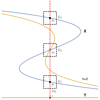
Figure 1: Demonstration of the neighborhoods $U_{i}$. $U_{1}$ and $U_{2}$ are small enough, so $U_{0}\times U_{1}$ and $U_{0}\times U_{2}$ do not intersect with $V(h)$.

By Theorem 2.2, the continuity of roots in the coefficients, there is a neighborhood $U$ in $S$ of $\boldsymbol{y}$ such that for all $\boldsymbol{y}^{\prime}\in U$, the equation $f(\boldsymbol{y}^{\prime};x)=0$ has exactly $\mu_{i}$ solutions in $U_{i}$ (counted with multiplicity). By replacing $U$ with $U\cap U_{0}$ if necessary, we may assume that $U\times U_{i}$ is disjoint from the locus of $h(y,x)=0$ for $1\leq i\leq k$. Then we can conclude that for all $\boldsymbol{y}^{\prime}\in U:$ there are exactly $\mu_{i}$ solutions (counted with multiplicity) to $f(\boldsymbol{y}^{\prime};x)=0\wedge h(\boldsymbol{y}^{\prime};x)\neq 0$ in $U_{i}$ for $1\leq i\leq k$. But $\#(D(h))_{\overline{y}}=k$ is invariant on $S$, forcing that there is exactly 1 solution of multiplicity $\mu_{i}$ to $f(\boldsymbol{y}^{\prime};x)=0\wedge h(\boldsymbol{y}^{\prime};x)\neq 0$ in $U_{i}$ for $1\leq i\leq k$ and no solution in $U_{i}$ for $k+1\leq i\leq l$ at all. Also, for $e+1\leq i\leq k$, the root of $f(\boldsymbol{y}^{\prime};x)=0\wedge h(\boldsymbol{y}^{\prime};x)\neq 0$ in $U_{i}$ must be non-real because $U_{i}\cap R=\varnothing$. So for $1\leq i\leq e$, the root of $f(\boldsymbol{y}^{\prime};x)=0\wedge h(\boldsymbol{y}^{\prime};x)=0$ in $U_{i}$ is real, hence equal to the last coordinate of $\xi_{i}(\boldsymbol{y}^{\prime})$ (recall Theorem 4.2). This shows the continuity. ∎

To show our theory does generalize Collins’s original cylindrical algebraic decomposition, we will show that Collins’s Theorem 1 is a special case of Theorem 4.2 and 4.3.

Definition 4.4 (Collins’s Delineability).

Let $f(x_{1},\ldots,x_{r})\in R[x_{1},\ldots,x_{r}]\,(r\geq 2)$, and let $S\subseteq R^{r-1}$ be a semi-algebraic set. The roots of $f$ are delineable over $S$ and that $\xi_{1},\ldots,\xi_{k}\,(k\geq 0)$ delineate the real roots of $f$ over $S$ if the following conditions are satisfied:

1. There are $m\geq 0$ positive integers $\mu_{i}$ such that if $(a_{1},\ldots,a_{r-1})\in S$ then $f(a_{1},\ldots,a_{r-1},x)=0$ has exactly $m$ distinct roots (in $C$), with multiplicities $\mu_{1},\ldots,\mu_{m}$.

2. $\xi_{1}<\xi_{2}<\cdots<\xi_{k}$ are semi-algebraic continuous functions from $S$ to $R$.

3. If $(a_{1},\ldots,a_{r-1})\in S$ then $\xi_{i}(a_{1},\ldots,a_{r-1})$ is a root of $f(a_{1},\ldots,a_{r-1},x)=0$ of multiplicity $\mu_{i}$ for all $1\leq i\leq k$ and $(a_{1},\ldots,a_{r-1})\in S$.

4. If $(a_{1},\ldots,a_{r-1})\in S$, $b\in R$ and $f(a_{1},\ldots,a_{r-1},b)=0$ then $b=\xi_{i}(a_{1},\ldots,a_{r-1})$ for some $i$.

Corollary 4.5 (Collins cf.[18, Theorem 1]).

Let $f(x_{1},\ldots,x_{r})$ be an $R$-polynomial, $r\geq 2$. Let $S$ be a semi-algebraically connected semi-algebraic subset of $R^{r-1}$. If ${\mathtt{LC}}_{x_{r}}(f)$ has no zero on $S$ and the number of distinct roots of $f$ in $x_{r}$ is invariant on $S$, then the roots of $f$ are delineable on $S$.

Proof.

Set $A=R[x_{1},\ldots,x_{n-1}]$ and $B=R[x_{1},\ldots,x_{n}]/\langle f\rangle.$ Let $X=\mathop{\mathrm{Spec}}B$ and $Y=\mathop{\mathrm{Spec}}A$. There is a natural morphism $\pi:X\to Y$ induced by the ring map $R[x_{1},\ldots,x_{r-1}]\to R[x_{1},\ldots,x_{r}]/\langle f\rangle$. If $\deg_{x_{r}}(f)=0$ then we are already done. So let us suppose $\deg_{x_{r}}(f)>0$ and set $w={\mathtt{LC}}_{x_{r}}(f)$, then $B_{w}$ is a free $A_{w}$-module of finite rank (generated by monomials $1,x_{r},\ldots,x_{r}^{\deg_{x_{r}}(f)-1}$). The rest immediately follows from Theorem 4.3 (note that the constant multiplicity is implied in the proof of Theorem 4.3.) ∎

Motivated by Collins’s Delineability, we will define Geometric Delineability for a basic constructible set.

Definition 4.6 (Geometric Delineability I).

Let $T=V(f_{1},\ldots,f_{s})\cap D(h)$ be a basic constructible set in $\mathbb{A}^{n+1}_{R}$, where $f_{i},h\in R[x_{1},\ldots,x_{n+1}]$. Let $S$ be a semi-algebraically connected semi-algebraic set in $R^{n}$. We say $T$ is geometrically delineable over $S$, if the following conditions holds:

1. For all $a=(a_{1},\ldots,a_{n})\in S$, the number of distinct solutions (in $C$) of

   $$f_{1}(a;x_{n+1})=\cdots=f_{s}(a;x_{n+1})=0,\ h(a;x_{n+1})\neq 0$$

   is finite and invariant.

2. There are semi-algebraic continuous functions $\xi_{1},\ldots,\xi_{k}:S\to T(R)$ such that $\pi\circ\xi_{i}=\mathrm{id}_{S}$, where $\pi:A^{n+1}_{R}\to A^{n}_{R}$ is the projection map. Additionally, we can require $\xi_{i}$ to be arranged in strictly ascending order in the last coordinate.

3. If $t\in T(R)\cap(S\times R^{1})$, then there is some unique $1\leq i\leq k$ such that $t=\xi_{i}(\pi(t))$.

The semi-algebraic continuous functions $\xi_{i}$ are called the sections of $T$ over $S$.

We make the convention that if $T\cap(S\times R^{1})=D(h^{\prime})\cap(S\times R^{1})$ for some $h\in R[x_{1},\ldots,x_{n+1}]$, then we say $T$ is geometrically delineable over $S$ if $V(h^{\prime})$ is geometrically delineable over $S$, and the sections of $T$ over $S$ are defined to be the sections of $V(h^{\prime})$ over $S$.

Example 2 (Geometric Delineability Examples).

(a) Nodal Curve

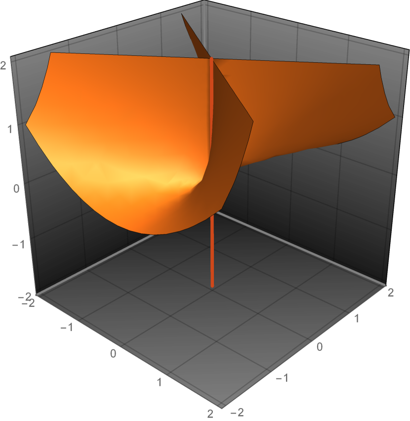
(b) Whitney Umbrella

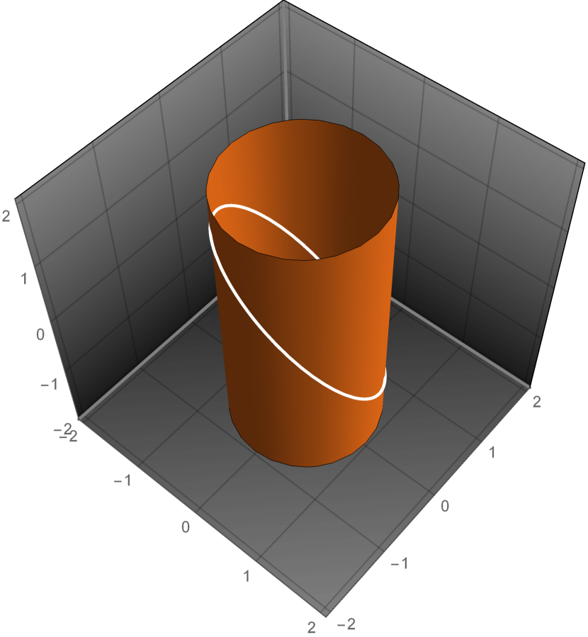
(c) Cylinder with an Ellipse Removed

Figure 2: Several Geometric Objects to Demonstrate Geometric Delineability

Figure 2(a) is the nodal curve $E:y^{2}-x^{2}(x+1)=0$ in $R^{2}$. Let $I_{1}=(-\infty,-1)$, $p_{1}=\{-1\}$, $I_{2}=(-1,0)$, $p_{2}=\{0\}$ and $I_{3}=(0,+\infty)$ be intervals or points in $R^{1}$. It is easy to see that $E$ is geometrically delineable over these subsets of $R^{1}$. For example, $E$ is geometrically delineable over $I_{2}$ because there are two different roots of $y^{2}-x^{2}(x+1)=0$ in $y$ when $x\in I_{2}$, given by $y=\pm\sqrt{x^{2}(x+1)}$.

Figure 2(b) is the Whitney’s umbrella $U:x^{2}-y^{2}z=0$ in $R^{3}$. Clearly $U$ is geometrically delineable over $\{(x,y)\in R^{2}|y\neq 0\}$ because $z=\frac{x^{2}}{y^{2}}$ over this region. Also $U$ is geometrically delineable over $\{(x,y)\in R^{2}|x\neq 0,y=0\}$ because there is no solution in $z$ when $y=0$ but $x\neq 0$. By the convention we made in Definition 4.6, $U$ is geometrically delineable over $\{(0,0)\}$ because the whole $z$-axis is contained in $U$, and $U\cap(\{(0,0)\}\times R^{1})=D(1)\cap(\{(0,0)\}\times R^{1})$. Clearly $\varnothing=V(1)$ is geometrically delineable over any sets.

Figure 2(c) is a cylinder with an ellipse removed $P:\left\{\begin{array}[]{rcl}x^{2}+y^{2}-1&=&0\\ x+y+z&\neq&0\end{array}\right.$ in $R^{3}$. Then $P$ is geometrically delineable over $F=\{(x,y)\in R^{2}|x^{2}+y^{2}-1=0\}$, because $P\cap(F\times R^{1})=D(x+y+z)\cap(F\times R^{1})$ and $V(x+y+z)$ is geometrically delineable over $F$ ($z=-x-y$).

We can rephrase Theorem 4.3 in our new terminology by just saying $D(h)\subseteq X$ is geometrically delineable over $S$.

Theorem 4.3 (Reformulation in Geometric Delineability).

If $\pi:X\to Y$ is a Projection of Relative Dimension 1 between affine $R$-varieties and $Y$ is integral. Suppose $W$ is a distinguished open in $Y$ such that $\pi|_{\pi^{-1}(W)}$ is finite and free, and $h\in\Gamma(X,\mathcal{O}_{X})$. Let $S\subseteq W(R)$ be a semi-algebraic connected semi-algebraic set such that $\#(D(h))_{\overline{y}}$ is invariant over $S$, then $D(h)$ is geometrically delineable over $S$.

Input: $I\unlhd k[\boldsymbol{y},x],J\unlhd k[\boldsymbol{y}],h\in k[\boldsymbol{y},x]$; Here, $k$ is a subfield of $R$, $J$ is a prime ideal such that $I\cap k[\boldsymbol{y}]\supseteq J$.

Output: Basic constructible sets $\{L_{i}\}$ in $R^{n}$ such that $V(I)\cap D(h)$ is geometrically delineable over semi-algebraically connected components of each $L_{i}$. Also, $\cup_{i}L_{i}=V(J)$.

1 if $1\in I$ then

2      return $\{V(J)\}$;

3Compute a reduced Gröbner basis $\mathcal{G}$ of $I$ w.r.t some block order $x>T_{\boldsymbol{y}}$;

4 if $I\cap k[\boldsymbol{y}]\neq J$ then

5       Decompose $V(J)\backslash V(I\cap k[\boldsymbol{y}])$ into basic constructible subsets $\{L_{i}\}$;

6       $J:=I\cap k[\boldsymbol{y}]$;

7       $\{J_{i}\}:=\mathtt{PrimeDecomposition}(J)$;

8       return $\{L_{i}\}\cup\bigcup_{i}\mathtt{Proj1}(J_{i}\cdot k[\boldsymbol{y},x]+I,J_{i},h)$;

9      

10if $\mathcal{G}\subseteq k[\boldsymbol{y}]$ then

11       return $\mathtt{Proj1}(I+\langle h\rangle,J,1)$;

12      

13$w:=\prod_{g\in\mathcal{G}\backslash J}{\mathtt{LC}}_{x}(g)$;

14 $s:=\min_{g\in\mathcal{G}\backslash J}\deg_{x}(g)$;

15 for $i:=0$ to $s-1$ do

16       for $j:=0$ to $s-1$ do

17             $(H_{h})_{i+1,j+1}:=\mathop{\mathrm{tr}}L_{x^{i+j}h}$;

18            

19      

20$\chi(\boldsymbol{y};\lambda):=\mathtt{CharacteristicPolynomial}(H_{h})$, written as $\chi(\boldsymbol{y};\lambda)=\sum_{i=0}^{s}c_{i}(\boldsymbol{y})\lambda^{i}$;

21 $L:=\varnothing$;

22 for $i:=0$ to $s-1$ do

23       $L:=L\cup\{V(J+\langle c_{0},\ldots,c_{i-1}\rangle)\cap D(w\cdot c_{i})\}$;

24      

25$\{J_{i}\}:=\mathtt{PrimeDecomposition}(J+\langle w\rangle)$;

26 return $L\cup\bigcup_{i}\mathtt{Proj1}(J_{i}\cdot k[\boldsymbol{y},x]+I,J_{i},h)$;

Algorithm 3 Proj1

We now describe Algorithm 3, which is very similar to Algorithm 1 (and its algebraic version Algorithm 2). So only the difference is explained.

1. Algorithm 3 also keeps tracks of the points having empty fiber in Line 3 and 3.

2. Algorithm 3 is greatly simplified when the morphism is not generically finite, see Line 3.

3. Algorithm 3 uses the coefficients of the characteristic polynomial of $H_{h}$, the Hermite Quadratic Form associated with $h$ in Line 3, instead of the minors of $H_{h}$.

Theorem 4.7.

Algorithm 3 terminates, and for all basic constructible sets $L$ in the output, $V(I)\cap D(h)$ is geometrically delineable over each semi-algebraically connected components of $L$.

Proof.

Termination. This part is almost identical to the proof of Theorem 3.7. The recursive calls in Line 3 and Line 3 run with larger ideals $J_{i}$. And we can discuss the recursive call in Line 3 in two cases:

1. $h\notin I$. Then $I+\langle h\rangle$ is a larger ideal.

2. $h\in I$. Then the call will actually be $\mathtt{PROJ1}(I,I\cap k[\boldsymbol{y}],1)$. So next time it will execute $\mathtt{PROJ1}(\langle 1\rangle,I\cap k[\boldsymbol{y}],1)$ and terminates.

Since $k[\boldsymbol{y},x]$ is noetherian, the algorithm certainly terminates.

Correctness. We still prove this on a case-by-case basis.

When $\pi:V(I)\to V(J)$ is not dominant, clearly $V(I)$ has empty fibers over $V(J)\backslash V(I\cap k[\boldsymbol{y}])$ and $V(I)\cap D(h)$ is obviously geometrically delineable over it. So Line 3 will keep track of it. Then the algorithm decomposes the image into irreducible components $V(J_{i})$ and restricts to $\pi^{-1}(V(J_{i}))\cap V(I)\to V(J_{i})$. Given a semi-algebraically connected semi-algebraic set $S$ contained in $V(J_{i})$, if $\pi^{-1}(V(J_{i}))\cap V(I)\cap D(h)$ is geometrically delineable over $S$ then by definition, $V(I)\cap D(h)$ is geometrically delineable over $S$. So our algorithm is correct in this case.

When $\pi:V(I)\to V(J)$ is dominant but not generically finite, then the Gröbner basis $\mathcal{G}$ is contained in $k[\boldsymbol{y}]$. This is because $\pi$ is a Projection of Relative Dimension 1, $V(I)=V(J)\times\mathbb{A}^{1}_{k}$ by Theorem 3.9. Now given a semi-algebraically connected semi-algebraic set $S$ contained in $V(J)$, we have that $V(I)\cap D(h)\cap(S\times R^{1})=D(h)\cap(S\times R^{1})$. So by the convention we made in Definition 4.6, it suffices to look at $V(I+\langle h\rangle)$ (see Line 3). Therefore our algorithm is also correct in this case.

When $\pi:V(I)\to V(J)$ is a generically finite, dominant morphism, we can compute $w\notin J$ such that $k[\boldsymbol{y},x]_{w}/I_{w}$ is a free $k[\boldsymbol{y}]_{w}/J_{w}$-module of finite rank by Theorem 3.4. Then for any $R$-rational point $p$ in $D(w)\cap V(J)$, the rank of the parametric Hermite Quadratic Form $H_{h}$ associated with $h$ evaluated at $p$ is uniquely determined by its characteristic polynomial, because $H_{h}(p)$ is a symmetric matrix with entries in $R$ and it is diagonalizable in $R$ (see [8, Theorem 4.43]). Moreover, suppose the characteristic polynomial is $\chi_{H_{h}(p)}(\lambda)=\sum_{i=0}^{s}c_{i}\lambda^{i}$, then $\mathop{\mathrm{rank}}H_{h}(p)=r$ if and only if $c_{0}=\cdots=c_{s-1-r}=0$ and $c_{s-r}\neq 0$. This justifies Line 3. By Lemma 3.1, Theorem 4.2 and 4.3, if $S\subseteq V(J)\cap D(w)$ is a semi-algebraically connected semi-algebraic set that $\mathop{\mathrm{rank}}H_{h}(p)$ is invariant for all $p\in S$, then $V(I)\cap D(h)$ is geometrically delineable over $S$. At last, the algorithm makes recursive calls to handle the non-free locus. The proof is completed. ∎

4.2 The Projection Phase

In this subsection we will build an analogue to Hoon’s improved Projection Operator [36]. We now extends Geometric Delineability to multiple basic constructible sets, just as Collins extended his delineability to multiple polynomials.

Definition 4.8 (Geometric Delineability II).

A family of basic constructible sets $\{L_{i}\}_{i=1}^{l}$ in $R^{n+1}$ is said to be geometrically delineable over a semi-algebraically connected semi-algebraic set $S\subseteq R^{n}$, if each $L_{i}$ is geometrically delineable over $S$, and all the sections of $L_{i}$ ($i=1,\ldots,l$) are either identical or disjoint. As a consequence, the set of sections $\{\xi_{ij}:S\to R^{n+1}\}$ can be sorted in strictly ascending order in the last coordinate.

We explain our settings in this subsection:

1. Let $X\to Y$ be a generically finite Projection of Relative Dimension 1 between $R$-varieties with $Y$ integral.

2. Open subscheme $W=D(w)$ is a distinguished open of $Y$ such that $X_{W}\to W$ is finite and free, where $X_{W}$ is the fiber product $X\times_{Y}W$ (by generic freeness).

3. Let $Z$ be a closed subscheme of $X_{W}$ and suppose $U=Z_{h^{\prime}}=D(h^{\prime})$ is a distinguished open in $Z$ for some $h^{\prime}\in\mathcal{O}_{Z}(Z)$. Let $V$ be the scheme-theoretical image of $U$ in $W$, so we have the following commutative diagram [34, Exercise II.3.11(d)]. We require $V$ to be integral in addition.

4. Choose $v\in\mathcal{O}_{V}(V)$ such that $U_{v}=V_{v}\times_{V}U\to V_{v}$ is free, where $V_{v}$ is the distinguished open in $V$ defined by $v$ (again by generic freeness).

5. Finally, let $h\in\Gamma(X,\mathcal{O}_{X})$ and $D(h)$ is the distinguished open in $X$ cut out by $h$. Also, let $(X_{W})_{h}$, $Z_{h}$, $U_{h}$ and $U_{hv}$ be the distinguished opens cut out by $h$ in $X_{W}$, $Z$, $U$ and $U_{v}$ respectively. They can be obtained by successive fiber products.

We have the following commutative diagram:

The following result, commonly referred as Stickelberger’s Eigenvalue Theorem, is needed to prove Theorem 4.10. A proof can be found in [15, Prop. 2.7] or [8, Theorem 4.99]. Cox also wrote an article about the history of Stickelberger’s Eigenvalue Theorem [20].

Lemma 4.9 (Stickelberger).

If $J$ is a zero-dimensional ideal in $C[x_{1},\ldots,x_{n}]$ and $f\in C[x_{1},\ldots,x_{n}]$, then

$$\det(\lambda I-L_{f})=\prod_{p\in V(J)}(\lambda-f(p))^{m(p)},$$

where $m(p)$ is the multiplicity of $p$ in $V(J)$ and $L_{f}$ is the multiplication of $f$ in $C[x_{1},\ldots,x_{n}]/J$.

Then the following theorem and its corollary are the analogues of [36, Lemma 3].

Theorem 4.10.

Let $S\subseteq V_{v}(R)$ be a semi-algebraically connected semi-algebraic set. Suppose for all $y\in S$, $\#(D(h))_{\overline{y}}$ is invariant, then $\#{(U_{h})}_{\overline{y}}$ is also invariant. As a corollary, $\#(\pi_{0}|_{U_{h}}^{-1}(y))$ is invariant over $S$ and there are semi-algebraic continuous sections $\xi_{i}:S\to U_{h}(R)$ that cover the preimage of $S$. In other words, $U_{h}$ is geometrically delineable over $S$.

Proof.

Again, we present our goal in the following diagram:

We can repeat the proof of Theorem 4.3 here. Let $Y=\mathop{\mathrm{Spec}}A$, $X=\mathop{\mathrm{Spec}}B$, then $W=\mathop{\mathrm{Spec}}A_{w}$ for some $w\in A$ and $X_{W}$ is the spectrum of $B_{w}=A_{w}\otimes_{A}B=A_{w}[x]/\langle f\rangle$ for some $f\in A_{w}[x]$ by Lemma 3.10. So for all $\boldsymbol{y}\in W(R)$, the geometric fiber $(D(h))_{\overline{\boldsymbol{y}}}$ corresponds to the solutions of $f(\boldsymbol{y};x)=0\wedge h(\boldsymbol{y};x)\neq 0$.

Since $Z$ is a closed subscheme of the affine scheme $X_{W}$, $Z=\mathop{\mathrm{Spec}}B_{w}/J$ for some $J\unlhd B_{w}$ and $V=\mathop{\mathrm{Spec}}A_{w}/p$, where $p$ is the kernel of the ring map $A_{w}\to B_{w}\to B_{w}/J\to(B_{w}/J)_{h^{\prime}}$. Because $X_{W}\to W$ is a finite morphism, $Z\to W$ is necessarily a finite morphism. Then it is easy to see that $U\to V$ is quasi-finite (the fibers must be finite!) So as a consequence of another application of generic freeness, let $\mathcal{S}=(A_{w}/p)_{v}$ and $\mathcal{S}^{\prime}=(B_{w}/J)_{h^{\prime}v}$ (notice that $V_{v}=\mathop{\mathrm{Spec}}\mathcal{S}$ and $U_{v}=\mathop{\mathrm{Spec}}\mathcal{S}^{\prime}$), then $\mathcal{S}^{\prime}$ is an $\mathcal{S}$-algebra that is also a free $\mathcal{S}$-module of finite rank.

Therefore the left multiplication of $x\in\mathcal{S}^{\prime}$ is an $\mathcal{S}$-module endomorphism.

$$L_{x}:\begin{array}[]{rcl}\mathcal{S}^{\prime}&\to&\mathcal{S}^{\prime}\\ s&\mapsto&x\cdot s.\end{array}$$

By the Cayley-Hamilton Theorem [26, Theorem 4.3], $g(\lambda)=\det(\lambda I-L_{x})\in\mathcal{S}[\lambda]$ is a monic polynomial that nullifies $x$ in $\mathcal{S}^{\prime}$.

Now let $y\in\mathop{\mathrm{Spec}}S$, $S^{\prime}\otimes_{S}\kappa_{y}\otimes\overline{\kappa_{y}}$ is a zero-dimensional $\overline{\kappa_{y}}$-algebra. By Stickelberger’s Eigenvalue Theorem (Lemma 4.9),

$$\det(\lambda I-L_{x})=\prod_{p\in(U_{v})_{\overline{y}}}(\lambda-x(p)).$$

So for all $\boldsymbol{y}\in V_{v}(R)$, the geometric fiber $(U_{h})_{\overline{\boldsymbol{y}}}$ corresponds to the solutions of $g(\boldsymbol{y};x)=0\wedge h(\boldsymbol{y};x)\neq 0$.

Fix $\boldsymbol{y}\in S$. Let $(D(h))_{\overline{\boldsymbol{y}}}=\{x_{1},\ldots,x_{m}\}$ and $\deg x_{i}=\mu_{i}$ (as irreducible components). We can identify $x_{i}$ with a point $(\boldsymbol{y},\lambda_{i})$ in $R^{n}\times C$ and choose disjoint neighborhoods $E_{i}$ of $\lambda_{i}$ respectively (in Euclidean topology). Because $(U_{h})_{\overline{\boldsymbol{y}}}$ is a subscheme of $(D(h))_{\overline{\boldsymbol{y}}}$, by renumbering the points if necessary, we may assume $(U_{h})_{\overline{\boldsymbol{y}}}=\{x_{1},\ldots,x_{l}\}$ and $\deg x_{i}=\mu_{i}^{\prime}$. Applying the Continuity of Roots to $f$ and $g$ (Theorem 2.2), we can show that, when $E_{i}$ are small enough, there is an Euclidean neighborhood $E$ in $S$ of $\boldsymbol{y}$ such that for all $\boldsymbol{y}^{\prime}\in E$: $(D(h))_{\overline{\boldsymbol{y}^{\prime}}}$ has exactly $\mu_{i}$ points (counted with degree) in $\{\boldsymbol{y}^{\prime}\}\times E_{i}$ for $1\leq i\leq m$, and $(U_{h})_{\overline{\boldsymbol{y}^{\prime}}}$ has exactly $\mu_{i}^{\prime}$ points (also counted with degree) in $\{\boldsymbol{y}^{\prime}\}\times E_{i}$ for $1\leq i\leq l$ (Figure 1 is helpful here again).

Since $\#(D(h))_{\overline{\boldsymbol{y}}}$ is invariant, $(D(h))_{\overline{\boldsymbol{y}^{\prime}}}$ can only have one point of degree $\mu_{i}$ in $\{\boldsymbol{y}^{\prime}\}\times E_{i}$ ($1\leq i\leq m$). Because $(U_{h})_{\overline{\boldsymbol{y}^{\prime}}}$ is a subscheme of $(D(h))_{\overline{\boldsymbol{y}^{\prime}}}$, $(U_{h})_{\overline{\boldsymbol{y}^{\prime}}}$ have only one point of degree $\mu_{i}^{\prime}$ in $\{\boldsymbol{y}^{\prime}\}\times E_{i}$ ($1\leq i\leq l$). By comparing degrees, $U_{\overline{\boldsymbol{y}^{\prime}}}$ has no other points. So $\#(U_{h})_{\overline{y^{\prime}}}=m$ for all $y^{\prime}\in E$. In other words, $\#(U_{h})_{\overline{y^{\prime}}}$ is locally constant. Since $\#(U_{h})_{\overline{y^{\prime}}}$ is a semi-algebraic function (the argument is similar to Lemma 4.1), $\#(U_{h})_{\overline{y^{\prime}}}$ is invariant on $S$ by Lemma 2.1. The rest follows from Theorem 4.3. ∎

Corollary 4.11.

Suppose $X^{\prime}\hookrightarrow\mathbb{A}_{R}^{n+1}$ is another closed subscheme and $Z=X_{W}\cap X^{\prime}$. If $X\cap D(h)$ and $X^{\prime}\cap D(h^{\prime})$ are geometrically delineable over $S$, then $\{X\cap D(h),X^{\prime}\cap D(h^{\prime})\}$ is geometrically delineable over $S$.

In addition, if $L=(X\cap D(h))\cup(X^{\prime}\cap D(h^{\prime}))$ is again a basic constructible subset in $\mathbb{A}_{R}^{n+1}$, then $L$ is geometrically delineable over $S$.

Proof.

It suffices to show the sections of $X\cap D(h)$ and $X^{\prime}\cap D(h^{\prime})$ are either identical or disjoint. By Theorem 4.10, $U_{h}$ is geometrically delineable over $S$. It remains to show

$$U_{h}\cap(V_{v}\times_{R}\mathbb{A}_{R}^{1})=(X\cap D(h))\cap(X^{\prime}\cap D(h^{\prime}))\cap(V_{v}\times_{R}\mathbb{A}_{R}^{1}),$$

so the sections of $U_{h}$ are all the common sections of $X\cap D(h)$ and $X^{\prime}\cap D(h^{\prime})$ over $S$. Apparently other sections of $X\cap D(h)$ and $X^{\prime}\cap D(h^{\prime})$ are disjoint.

Notice that $Z=X_{W}\cap X^{\prime}$, so $U=X_{W}\cap X^{\prime}\cap D(h^{\prime})$ and $U_{h}=D(h)\cap X_{W}\cap X^{\prime}\cap D(h^{\prime})$. Then

$$U_{h}\cap(V_{v}\times\mathbb{A}_{R}^{1})=((X_{W}\cap D(h))\cap(X^{\prime}\cap D(h^{\prime}))\cap(V_{v}\times_{R}\mathbb{A}_{R}^{1})).$$

But $V_{v}$ is contained in $W$ and $X_{W}=X\cap(W\times_{R}\mathbb{A}_{R}^{1})$. Therefore the geometric delineability of $X\cap D(h),X^{\prime}\cap D(h^{\prime})$ and $U_{h}$ over $S$ implies the geometric delineability of $\{X\cap D(h),X^{\prime}\cap D(h^{\prime})\}$ over $S$.

If their union $L$ is locally closed, then the sections of $X\cap D(h)$ and $X^{\prime}\cap D(h^{\prime})$ are the sections of $L$. And

$$\#L_{\overline{y}}=\#(X\cap D(h))_{\overline{y}}+\#(X^{\prime}\cap D(h^{\prime}))_{\overline{y}}-\#(U_{h})_{\overline{y}}$$

is invariant on $S$. Therefore $L$ is geometrically delineable over $S$. ∎

Input: $I_{0}\unlhd k[\boldsymbol{y},x]$, $J_{0}\unlhd k[\boldsymbol{y}]$, $h^{\prime},w\in k[\boldsymbol{y},x]$; $I_{0}$ satisfies that $I_{0}\cap k[\boldsymbol{y}]\supseteq J_{0}$ and $J_{0}$ is prime.

Output: A list of basic constructible sets $\{L_{i}\}$.

1 Introduce a new variable $z$, compute the reduced Gröbner Basis $\mathcal{G}$ of $I_{0}\cdot k[\boldsymbol{y},x,z]+\langle z\cdot h^{\prime}-1\rangle$ w.r.t. $T_{x,z}>T_{\boldsymbol{y}}$;

2 if $1\in I_{0}$ then

3      return $\varnothing$;

4if $I_{0}\cap k[\boldsymbol{y}]\neq J_{0}$ then

5       $\{J_{i}\}:=\mathtt{PrimeDecomposition}(I_{0}\cap k[\boldsymbol{y}])$;

6       return $\bigcup_{i}\mathtt{Proj2Sub}(I_{0}+J_{i}\cdot k[\boldsymbol{y},x],J_{i},h^{\prime},w)$;

7      

8$v:=\prod_{g\in\mathcal{G}\backslash J_{0}}{\mathtt{LC}}_{T_{x,z}}(g)$;

9 $\{J_{i}\}:=\mathtt{PrimeDecomposition}(J_{0}+\langle v\rangle)$;

10 return $\{(J_{0},w\cdot v)\}\cup\bigcup_{i}\mathtt{Proj2Sub}(I_{0}+J_{i}\cdot k[\boldsymbol{y},x],J_{i},h^{\prime},w)$;

Algorithm 4 Proj2Sub

Input: $I,I^{\prime}\unlhd k[\boldsymbol{y},x]$, $J\unlhd k[\boldsymbol{y}]$, $h,h^{\prime}\in k[\boldsymbol{y},x]$; $I\cap k[\boldsymbol{y}]\supseteq J$ and $J$ is prime.

Output: A list of basic constructible sets $\{L_{i}\}$, satisfying if $S$ is a semi-algebraically connected semi-algebraic set contained in some $L_{i}$ and $V(I)\cap D(h)$, $V(I^{\prime})\cap D(h^{\prime})$ are geometrically delineable over $S$, then $\{V(I)\cap D(h),V(I^{\prime})\cap D(h^{\prime})\}$ is geometrically delineable over $S$.

1 Compute a reduced Gröbner Basis $\mathcal{G}$ of $I$ w.r.t. $x>T_{\boldsymbol{y}}$;

2 if $1\in I$ then

3      return $\varnothing$;

4if $I\cap k[\boldsymbol{y}]\neq J$ then

5       $\{J_{i}\}:=\mathtt{PrimeDecomposition}(I\cap k[\boldsymbol{y}])$;

6       return $\bigcup_{i}\mathtt{Proj2}(I+J_{i}\cdot k[\boldsymbol{y},x],I^{\prime},J_{i},h,h^{\prime})$;

7      

8if $I=J\cdot k[\boldsymbol{y},x]$ then

9       return $\mathtt{Proj2}(I+\langle h\rangle,I^{\prime},J,1,h^{\prime})$;

10      

11$w:=\prod_{g\in\mathcal{G}\backslash J}{\mathtt{LC}}_{x}(g)$;

12 $\{J_{i}\}:=\mathtt{PrimeDecomposition}(J+\langle w\rangle)$;

13 return $\mathtt{Proj2Sub}(I+I^{\prime},\langle 0\rangle,h^{\prime},w)\cup\bigcup_{i}\mathtt{Proj2}(I+J_{i}\cdot k[\boldsymbol{y},x],I^{\prime},J_{i},h,h^{\prime})$;

Algorithm 5 Proj2

Input: A list of basic constructible sets $\{L_{i}\}_{i=1}^{s}$, each $L_{i}$ is given by an ideal $I_{i}$ and a polynomial $h_{i}$ such that $L_{i}=V(I_{i})\cap D(h_{i})$.

Output: A list of basic constructible sets. See Theorem 4.13.

1 $ret=\{\}$;

2 for $i:=1$ to $s$ do

3       $ret:=ret\cup\mathtt{Proj1}(I_{i},\langle 0\rangle,h_{i})$;

4      

5for $i:=1$ to $s$ do

6       for $j:=1$ to $i-1$ do

7            $ret:=ret\cup\mathtt{Proj2}(I_{i},I_{j},\langle 0\rangle,h_{i},h_{j})$;

8      

9return $ret$;

Algorithm 6 CADProjection

Theorem 4.12.

Algorithm 5 is correct and terminates.

Proof.

Termination. Almost the same as Algorithm 3. See Theorem 4.7.

Correctness. The second if-statement tests whether the morphism $V(I)\to V(J)$ is dominant. If not, the algorithm replaces $J$ with its irreducible components (with the reduced induced scheme structure) and recursively calls $\mathtt{Proj2}$. This part is obviously correct (restricting on the base does not matter).

The third if-statement tests whether the morphism is generically finite. If not, then $V(I)=V(J)\times\mathbb{A}_{k}^{1}$ and we must replace $V(I)\cap D(h)$ with $V(I+\langle h\rangle)$. Recall Definition 4.6 and 4.8, we see that “$\{D(h),V(I^{\prime})\cap D(h^{\prime})\}$ is geometrically delineable over $S\subseteq V(J)$” is equivalent to “$\{V(I+\langle h\rangle),V(I^{\prime})\cap D(h^{\prime})\}$ is geometrically delineable over $S\subseteq V(J)$”.

If all the three if-statements are passed, then $V(I)\to V(J)$ is a dominant generically finite Projection of Relative Dimension 1 with $J$ prime, playing the role of $X\to Y$. The next line constructs the generic freeness, which corresponds to $W$ and $X_{W}$.

Then the algorithm calls Algorithm 4 with $V(I+I^{\prime})\to\mathbb{A}_{R}^{n}$. Algorithm 4 does the same test, and when all the if-statements are passed, we have $Z=V(I_{0})\cap(W\times\mathbb{A}_{R}^{1})$, $U=Z\cap D(h^{\prime})$, $V=V(J_{0})\cap W$ and $V$ is the scheme-theoretical image of $U$. Then the algorithm computes $v$ to construct generic freeness again. Suppose $S\subseteq V_{v}(R)$ is a semi-algebraically connected semi-algebraic set that $V(I)\cap D(h)$ and $V(I^{\prime})\cap D(h^{\prime})$ are geometrically delineable, then by Corollary 4.11, $\{V(I)\cap D(h),V(I^{\prime})\cap D(h^{\prime})\}$ is geometrically delineable over $S$. The last recursive calls in Algorithm 4 and 5 deal with the part where the generic freeness fails.

∎

Theorem 4.13.

Let $\{L_{i}\}_{i=1}^{l}$ be a list of basic constructible sets in $R^{n+1}$, and $\{L_{i}^{\prime}\}_{i=1}^{l^{\prime}}=\mathtt{CADProjection}(\{L_{i}\}_{i=1}^{l})$ (see Algorithm 6). If $S\subseteq R^{n}$ is a semi-algebraically connected semi-algebraic set satisfying for each $L_{i}^{\prime}$: either $S\subseteq L_{i}^{\prime}$ or $S\cap L_{i}^{\prime}=\varnothing$. Then $\{L_{i}\}_{i=1}^{l}$ is geometrically delineable over $S$.

Proof.

It is clear that $\{L_{i}^{\prime}\}$ contains all the outputs of $\mathtt{Proj1}$ (Algorithm 3). So by Theorem 4.7, each $L_{i}$ is geometrically delineable over $S$. By the definition of geometric delineability 4.8, it remains to prove $\{L_{i},L_{j}\}$ is geometrically delineable over $S$ for each pair $(i,j)$ $(1\leq j<i\leq l)$.

If $S$ is contained in some $L_{i}^{\prime}$ in the output of $\mathtt{Proj2}(I_{i},I_{j},\langle 0\rangle,h_{i},h_{j})$, then we are done by Corollary 4.11 and Theorem 4.12. Therefore we need to carefully analyze the output of $\mathtt{Proj2}$ to prove that, when $S$ is disjoint from all outputs of $\mathtt{Proj2}(I_{i},I_{j},\langle 0\rangle,h_{i},h_{j})$, $\{L_{i},L_{j}\}$ is still geometrically delineable over $S$.

Actually, we will prove that, if $p\in R^{n}$ is not contained in the output of $\mathtt{Proj2}(I_{i},I_{j},\langle 0\rangle,h_{i},h_{j})$, then the sections of $L_{i}$ and $L_{j}$ over $p$ are disjoint. To see this, we observe that the points missing in the output of $\mathtt{Proj2}$ is due to

1. [Algorithm 5, Line 5]. Because $I=\langle 1\rangle$, there is no section of $V(I_{i})$ over $V(J)$.

2. [Algorithm 5, Line 5]. Because $\overline{\pi(V(I))}=V(I\cap k[\boldsymbol{y}]),$ there is no section of $V(I_{i})$ over $V(J)\backslash V(I\cap k[\boldsymbol{y}])$.

3. [Algorithm 4, Line 4]. There is no section of $V(I_{i})\cap V(I_{j})\cap D(h_{j})$ over $V(J)$.

4. [Algorithm 4, Line 4]. There is no section of $V(I_{i})\cap V(I_{j})\cap D(h_{j})$ over $V(J)\backslash\overline{\pi(V(I)\cap D(h_{j}))}$.

So if $S$ is disjoint from the output of $\mathtt{Proj2}$, the sections of $V(I_{i})\cap D(h_{i})$ and $V(I_{j})\cap D(h_{j})$ are disjoint, and $\{L_{i},L_{j}\}$ is still geometrically delineable over $S$. ∎

The following lemma is extremely helpful to reduce the computation needed.

Lemma 4.14.

Suppose $V(f)\subseteq\mathbb{A}_{R}^{n+1}$ is covered by basic constructible subsets $L_{1}\ldots,L_{s}$, and for each $1\leq k\leq s:\bigcup_{i=1}^{k}L_{k}$ is again a basic constructible subset. If $\{L_{1},\ldots,L_{s}\}$ is geometrically delineable over a semi-algebraically connected semi-algebraic set $S\subseteq R^{n}$, then $V(f)$ is geometrically delineable over $S$. Hence $D(f)$ is geometrically delineable over $S$.

Proof.

Nothing but successively applying Corollary 4.11 to $L_{1}\cup L_{2}$, $(L_{1}\cup L_{2})\cup L_{3}$, $((L_{1}\cup L_{2})\cup L_{3})\cup L_{4}$, $\ldots$. ∎

4.3 The Lifting Phase

We assume the existence of an algorithm $\mathtt{Partition1D}$ that partition $R^{1}$ into intervals and points such that a given collection of polynomials is sign-invariant on each point and each interval. This can be achieved by the real root isolation algorithm when $R$ is archimedean (see [8, Algorithm 10.55]) and Thom Encoding if $R$ is a general real closed field (see [8, Algorithm 10.105, 10.106]).

We shall define cylindrical algebraic decomposition now. Our definition is almost the same as [8, Definition 5.1], but some adjustments are made.

Definition 4.15.

A cylindrical algebraic decomposition (abbreviated as CAD) of a finite set of semi-algebraic sets $\{L_{1},\ldots,L_{s}\}$ in $R^{n}$, is a sequence $S_{1},\ldots,S_{n}$, where for each $1\leq i\leq n$:

1. The set $S_{i}$ consists of semi-algebraic sets in $R^{i}$, which are called the cells of level $i$.

2. Each cell of level $1$ is either a point or an interval.

3. Each $L_{i}$ is a union of level $n$ cells. And for each cell $S\in S_{n}$ of level $n$ and each basic constructible set $L_{i}$, either $S\subseteq L_{i}$ or $S\cap L_{i}=\varnothing$.

4. For every $1<i\leq n$, and every $S\in S_{i}$, the “silhouette”

   $$\pi_{i-1}(S)={(y_{1},\ldots,y_{i-1}\in R^{i-1}|\exists x\in R\text{ s.t. }(y_{1},\ldots,y_{i-1},x)\in S)}$$

   is a cell of level $i-1$.

5. For every $1\leq i<n$, and every $S\in S_{i}$, there are finitely many semi-algebraic continuous functions $\xi_{S,1},\ldots,\xi_{S,l_{S}}:S\to R$ (the sections) such that the any cell in $S_{i+1}$ lying over $S$ is either the graph of some $\xi_{S,j}$

   $$\left\{(y,\xi_{S,j}(y))\in S\times R\middle|y\in S\right\},$$

   or the band

   $$\left\{(y,x)\in S\times R\middle|y\in S,\ \xi_{S,j}(y)<x<\xi_{S,j+1}(y)\right\},$$

   where we take $\xi_{S,0}(x)=-\infty$ and $\xi_{S,l_{S}+1}(x)=+\infty$.

Suppose $\{F_{i}\}$ is a finite set of basic constructible sets in $\mathbb{A}_{R}^{n}$, then their $R$-rational points $F_{i}(R)$ are semi-algebraic sets, and a cylindrical algebraic decomposition of $\{F_{i}\}$ is just a cylindrical algebraic decomposition of $\{F_{i}(R)\}$.

Theorem 4.16.

Suppose $\{L_{i}\}$ is a finite set of locally closed subsets in $\mathbb{A}_{R}^{n}$. A cylindrical algebraic decomposition of $\mathtt{CADProjection}(\{L_{i}\})$ (Algorithm 6) can be lifted to a cylindrical algebraic decomposition of $\{L_{i}\}$.

Proof.

Observe that cells in a cylindrical algebraic decomposition are always semi-algebraically connected, because a cell of level $>1$ is either a graph of a semi-algebraic continuous function defined over its silhouette, or a band between two graphs and a cell of level $1$ is either an interval or a point, now use induction. Then Theorem 4.13 shows that $\{L_{i}\}$ is geometrically delineable over each cell of level $n-1$. Take the sections and the bands as cells of level $n$ and it is easy to see these cells are either contained in $L_{i}(R)$ or disjoint from $L_{i}(R)$ for any $L_{i}$. The proof is completed. ∎

It is time to introduce the Geometric Cylindrical Algebraic Decomposition Algorithm (Algorithm 7).

Input: A list of basic constructible sets $\{L_{i}\}_{i=1}^{s}$ in $\mathbb{A}_{R}^{n}$, each $L_{i}$ is given by an ideal $I_{i}$ and a polynomial $h_{i}$ such that $L_{i}=V(I_{i})\cap D(h_{i})$.

Output: A cylindrical algebraic decomposition of $\{L_{1},\ldots,L_{s}\}$.

1 $\mathtt{precells}[n]:=\{L_{i}\}_{i=1}^{s}$;

2 for $i:=n-1$ downto $1$ do // Projection Phase

3       $\mathtt{precells}[i]:=\mathtt{CADProjection}(\mathtt{precells}[i+1])$;

4      

5$\mathtt{polys}:=$Polynomials defining $\mathtt{precells}[1]$;

6 $\mathtt{cells}[1]:=\mathtt{Partition1D}(\mathtt{polys})$;

7 for $i:=2$ to $n$ do // Lifting Phase

8       $\mathtt{cells}[i]:=\varnothing$;

9       for $S$ in $\mathtt{cells}[i-1]$ do

10             $\{\xi_{S,j}\}_{j=1}^{l_{S}}:=$The sections of $\mathtt{precells}[i]$ over $S$, additionally set $\xi_{S,0}:=-\infty$, $\xi_{S,l_{S}+1}=+\infty$;

11             Append $\{(y,\xi_{S,j}(y))|y\in S\}$ to $\mathtt{cells}[i]$ for all $1\leq j\leq l_{S}$;

12             Append $\{(y,x)|y\in S,\xi_{S,j}(y)<x<\xi_{S,j+1}\}$ to $\mathtt{cells}[i]$ for all $0\leq j\leq l_{S}$;

13            

14      

15return $\mathtt{cells}$;

Algorithm 7 GeometricCAD

Remark 7.

We remark that it is not necessary to append all sections and all bands to $\mathtt{cells}[i]$ in Algorithm 7. In fact, one can append the sections and bands contained in some $\mathtt{precells}[i]$. We are doing so just because this will give a partition of the whole real space $R^{i}$, as the Collins CAD does.

Remark 8.

The correctness of Algorithm 7 is obvious. Because $\mathtt{Partition1D}$ can generate a cylindrical algebraic decomposition of $\mathtt{precells}[1]$, using all the defining equations. Then Theorem 4.16 guarantees the correctness of lifting.

5 Applications of Geometric Cylindrical Algebraic Decomposition

In this section, we will show some applications of the Geometric Cylindrical Algebraic Decomposition. In principle, these problems can also be solved by the traditional CAD (Collins’s and its variants), but we hope the examples can help readers understand our new theory and show the difference between the traditional CAD and the Geometric CAD.

5.1 Real Root Classification

Just like the complex root classification problem in Section 3, we are also interested in the real root classification problem. Namely, given two semi-algebraic sets $S,T$ and a semi-algebraic map $\varphi:S\to T$, describe the region of each fiber in $T$ with a given cardinality.

This can be handled by Geometric CAD in the following way. Since we can always embed $S$ and $T$ in real spaces $R^{n}$ and $R^{m}$ ($n>m$) in the way that $\varphi:S\to T$ is the restriction of the projection map $R^{n}\to R^{m}$, we are reduced to counting the cardinality of fibers of $\varphi:S\subseteq R^{n}\to R^{m}$.

Now build a cylindrical algebraic decomposition of $S$. For each cell $S^{\prime}$ of level $m$, if there is a cell $S^{\prime\prime}$ of level $n$ contained in $S$ such that $\dim S^{\prime}<\dim S^{\prime\prime}$, then each fiber over $S^{\prime}$ is of cardinality $+\infty$. Else every cell of level $n$ lying over $S^{\prime}$ and contained in $S$ is of dimension $\dim S^{\prime}$, suppose there are $r$ cells lying over $S^{\prime}$, contained in $S$, then each fiber over $S^{\prime}$ has a cardinality of $r$.

Example 3.

Let $x^{3}+px+q=0$ be the depressed cubic equation in unknown $x$. When does it have 1, 2, or 3 real roots?

Using Algorithm 7, we build a CAD of $\{(p,q,x)\in R^{3}|x^{3}+px+q=0\}$. The algorithm goes as:

1. Projection phase, the first stage. There is only one set, so we need only $\mathtt{Proj1}(\langle x^{3}+px+q\rangle,\langle 0\rangle,1)$. The result is as illustrated below (empty sets omitted).

2. By Lemma 4.14, it suffices to look at the last two sets.

3. Projection phase, the second stage. Then we need to compute $\mathtt{Proj1}(\langle-4p^{3}-27q^{2}\rangle,\langle 0\rangle,6p-2p^{2}+4p^{3}+9q^{2})$, $\mathtt{Proj1}(\langle 4p^{3}+27q^{2},6p-2p^{2}+4p^{3}+9q^{2}\rangle,\langle 0\rangle,1)$ and $\mathtt{Proj2}$ between them. The results of $\mathtt{Proj1}$ is as shown below, and $\mathtt{Proj2}$ returns an empty list.

   So the defining polynomials are $p$ and $9-3p+4p^{2}$, which partition $R^{1}$ into three sets, $(-\infty,0)$,$\{0\}$ and $(0,\infty)$.

   Then the algorithm lifts the cylindrical algebraic decomposition to higher dimensions. The cells of level $2$ are listed by the figure below.

   One can draw a picture to demonstrate the cells of level $3$ too, but we do not continue due to space reasons. Anyway, it can be easily checked that the cells of level $2$ marked by a single $*$ are the regions that $x^{3}+px+q=0$ has only one real root. Similarly, the cells of level $2$ marked by double (triple, respectively) $*$ are the regions that $x^{3}+px+q=0$ has two (three respectively) real roots. This is equivalent to the classical criterion taught in undergraduate algebra:

   $$\#\{x\in R|x^{3}+px+q=0\}=\left\{\begin{array}[]{lr}3&4p^{3}+27q^{2}<0\\ 2&p<0\wedge 4p^{3}+27q^{2}=0\\ 1&\text{otherwise.}\end{array}\right.$$

5.2 The Decision Problem Over the Real Closed Field

Another application is to decide the truth value of a closed formula in the first order language of real closed fields. A closed formula in the first order language is a formula whose all variables are quantified. Readers may refer to [33] for basic concepts and terminologies in logic.

Suppose $\Phi=(Q_{1}x_{1})\cdots(Q_{n}x_{n})\phi(x_{1},\ldots,x_{n})$ is a closed formula in the first order language of real closed fields, where $Q_{i}\in\{\forall,\exists\}$, and $f_{1},\ldots,f_{s}$ are $R$-polynomials occurring in $\phi$. To decide the truth value of $\Phi$, it suffices to build a cylindrical algebraic decomposition of

$$\left\{V(f_{1}),\ldots,V(f_{s}),D(\prod_{i=1}^{s}f_{i})\right\},$$

using Algorithm 7.

Because every cell $S$ of level $n$ is semi-algebraically connected and for each $1\leq i\leq s$, either $S\subseteq V(f_{i})$ or $S\cap V(f_{i})=\varnothing$, we conclude that each $f_{i}$ is sign-invariant on $S$, which implies that $\phi(x_{1},\ldots,x_{n})$ is true for some $(x_{1},\ldots,x_{n})\in S$ if and only if that is true for all $x\in S$.

Since the cells are cylindrically arranged, let $T$ be a cell of level $n-1$ and $x^{\prime}=(x_{1},\ldots,x_{n-1})\in T$, $(\forall x_{n})\phi(x^{\prime},x_{n})$ holds if and only if all points in all cells $S$ of level $n$ lying over $T$ satisfy $\phi$. A similar conclusion can be drawn with the quantifier $\exists$. Therefore $(Q_{n}x_{n})\phi(x^{\prime},x_{n})$ is true for some $x^{\prime}\in T$ if and only if it is true for all $x^{\prime}\in T$.

By an induction on the dimension $n$, now it can be easily seen that the Geometric Cylindrical Algebraic Decomposition can be used to decide the first order theory of the real closed field.

Example 4.

Suppose one would like to know whether

$$(\forall p)(\forall q)(\exists x)(x^{3}+px+q=0)$$

holds. Obviously an $R$-polynomial of odd degree has a root in $R$, so we can use this to validate our algorithm.

We have already built a CAD for $x^{3}+px+q=0$ in Example 3, so let us continue the discussion there. Take the cell $\left\{(p,q)\in R^{2}\middle|p<0\wedge q=\sqrt{-\frac{4p^{3}}{27}}\right\}$ for example. There are 5 cells of level $3$ lying over it, two of them satisfy $x^{3}+px+q=0$. So this cell satisfies $(\exists x)(x^{3}+px+q=0)$. Do the same to other cells of level $2$, we have the following figure.

Finally, we see that $(\forall q)(\exists x)(x^{3}+px+q=0)$ is true for all cells of level $1$, thus we have that $(\forall p)(\forall q)(\exists x)(x^{3}+px+q=0)$ is true.

Example 5.

Here is another closed formula

$$(\forall p)(\forall q)(\exists x)(px+q=0).$$

Similarly build a cylindrical algebraic decomposition of $\{(p,q,x)\in R^{3}|px+q=0\}$ and do nearly the same discussion on the cells.

Therefore it is not true that for every $p,q\in R$, $px+q=0$ has a solution in $R$.

5.3 Quantifier Elimination

A Quantifier Elimination (QE) algorithm is an algorithm that takes a quantified sentence and returns a quantifier-free sentence that is equivalent to the input. That the theory of real closed fields admits Quantifier Elimination is proved by Tarski in [62], although the algorithm is highly inefficient. Collins’s CAD is the first practical Quantifier Elimination algorithm for $\mathbb{R}$.

Strictly speaking, our algorithm here does not directly eliminate quantifiers, because our cells are described by semi-algebraic continuous functions, which are generally not polynomials (see Example 3). However, it does have the ability of describing the regions in an extended language (so called “Extended Tarski Formula”). In other words, if we allow “root functions” in the language, then our algorithm can give a quantifier elimination procedure.

Collins’s original CAD can give a semi-algebraic description of the cells, using more polynomials ($\mathtt{APROJ}$, the augmented projection in [18]) and Thom’s Encoding, so it is able to do quantifier elimination. We will leave this topic to future researches, as this paper is lengthy enough.

5.4 Exploiting Constraints

One of the advantages of our algorithm is the geometric nature. Instead of building a CAD such that some given polynomials are sign-invariant in each cell of level $n$, we build a CAD of some constructible sets, so we can directly exploit some constraints in the problem. For example, suppose we are interested in the input formula

$$(f_{1}=0)\wedge\cdots\wedge(f_{s}=0)\wedge(h\neq 0)\wedge\phi$$

and $g_{1},\ldots,g_{t}$ are the polynomials defining $\phi$, then what happens outside

$$L=V(f_{1},\ldots,f_{s})\cap D(h)$$

is irrelevant here. So it suffices to build a CAD of $\{L\cap V(g_{1}),\ldots,L\cap V(g_{t}),L\cap D(\prod_{i=1}^{t}g_{i})\}$. Moreover, in the projection phase, we need only taking care of intersections of the sets and the “silhouette” of $L$. This can be done by computing a Gröbner basis for $\langle f_{1},\ldots,f_{s},z\cdot h-1\rangle$ with respect to the lexicographic order $x_{1}<\cdots<x_{n}<z$, then intersect every basic constructible set in $\mathtt{precells}[i]$ with the $i$-th elimination ideal. Also, in the lifting phase, we can append the relevant sections and bands only, see Remark 7.

In particular, this feature enables us to exploit multiple equational constraints in constructing CAD and this is certainly a new area worth exploring.

Example 6.

Let $f_{1}=x^{2}+y^{2}+z^{2}-1$, $f_{2}=2x-2y+z-1$, and $g=x+y+z+\frac{3}{2}$. Consider

$$\phi=(f_{1}=0)\wedge(f_{2}=0)\wedge(g<0).$$

By the previous discussion, we may exploit the constraint $(f_{1}=0)\wedge(f_{2}=0)$ and build a CAD of $\{V(f_{1},f_{2})\cap D(g),V(f_{1},f_{2},g)\}$.

Let $p_{1}=-4x+5x^{2}+4y-8xy+5y^{2}$, $p_{2}=5-2x+6y$, $p_{3}=85+188y+104y^{2}$, then the result of the first round of $\mathtt{CADProjection}(\{V(f_{1},f_{2})\cap D(g),V(f_{1},f_{2},g)\})$ is

$$\{D(p_{1}),V(p_{1})\cap D(p_{2}),V(p_{1},p_{2}),D(p_{2}),V(p_{2})\cap D(p_{3}),V(p_{2},p_{3})\}.$$

Because we are only interested in the silhouette of $L$ (which is $V(p_{1})$), we can reduce the results to

$$\{V(p_{1})\cap D(p_{2}),V(p_{1},p_{2})\}.$$

Then we perform the second round of $\mathtt{CADProjection}$, which gives basic constructible sets can be defined by two polynomials $-4-4x+9x^{2}$, $5+44x+104x^{2}$. These two polynomials partition $R^{1}$ into two points $\frac{1}{9}\left(2\pm 2\sqrt{10}\right)$ and three intervals.

Next we go to the lifting phase, Figure 3(a) shows cells of level 1 and 2. The ellipse is the locus of $p_{1}$ and the straight line is the locus of $p_{2}$, they are actually disjoint. Note that in the lifting phase we append sections and bands that are relevant, so there are only 4 cells of level 2. Continuing the lifting phase, there are only 4 cells of level 3 and $g$ is positive on all of them (see Figure 3(b)). So $\phi$ is unsatisfiable. In fact, the minimum of $g$ on $\{(x,y,z)\in R^{3}|f_{1}(x,y,z)=f_{2}(x,y,z)=0\}$ is $\frac{1}{18}\left(29-8\sqrt{13}\right)\approx 0.00864>0$. However, a CAD of $\{V(f_{1}),V(f_{2}),V(g),D(f_{1}f_{2}g)\}$ requires 1781 cells of level 3.

This example shows that when taking the constraints into consideration, the number of distinguished locally sets in the Projection Phase and the number of cells in the Lifting Phase can be dramatically decreased.

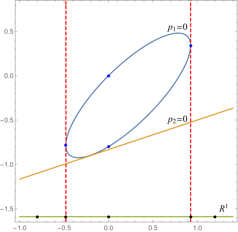
(a) Cells of level 1 and 2

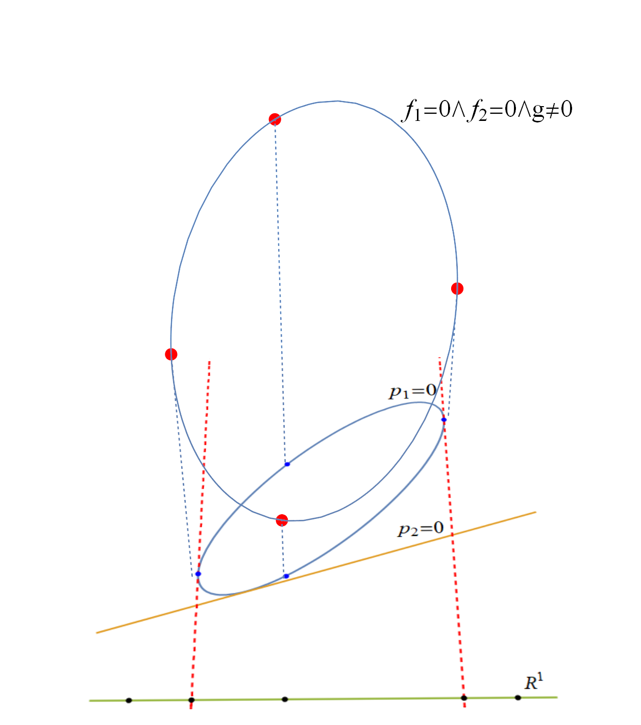
(b) Cells of level 3

Figure 3: The cylindrical algebraic decomposition in Example 6

6 Analysis

We have not included any complexity analysis because,

1. The decision problem over the real closed field is in  and it is also conjectured that this is -complete [7]. Moreover, it is shown in [22, 65, 2] that a cylindrical algebraic decomposition needs doubly-exponential number of cells in the worst case. So our algorithm probably does not improve the worst-case doubly-exponential bound of a cylindrical algebraic decomposition construction.

2. Our algorithm heavily relies on Gröbner Basis and it is certainly the most time-consuming part. But the complexity of Buchberger’s Algorithm is still not well understood in the geometric context. While the ideal membership problem is shown to be -complete [53, 48], Buchberger’s algorithm and its variants are often able to tackle problems of large size. In fact, there are many works to study why Gröbner basis computation is feasible in the cases of real interest in Algebraic Geometry, and sharper upper bounds are obtained by analyzing zero-dimensional systems [40, 44], low-dimensional systems [56, 57], regular sequences (Faugère’s F5) [27, 5].

3. Our theory is still in its preliminary form and there is much room for further improvements. It would be of better interest to analyze an improved version.

Still, an implementation of our algorithm is reported in A for interested readers. Although the implementation is still in a preliminary form, it can handle some problems that existing CAD methods cannot solve.

6.1 Connection to the Prior Work

We compare our theory to some other existing methods. We hope the following discussion can be inspiring and provide improvements to previous results. Please be aware that we do not claim our theory is superior to all others. In fact, it should be emphasized that our theory is far from being perfect and we hope the researchers from other related areas can join us to further develop this theory.

6.1.1 Collins’s Original CAD

It is very clear that our theory is deeply influenced by Collins’s work [18]. Both works are about cylindrical algebraic decomposition and our algorithm has a Projection Phase and a Lifting Phase, just as Collins’s does. Moreover, Algorithm 3 and 5 are analogues to Collins’s Projection and Hoon’s improvement [36].

However, the difference between our theory and Collins’s is apparent. The central object of study in our theory are (basic constructible) sets, while Collins’s is mainly about polynomials. Therefore the techniques used are quite different, the mathematics behind Collins’s work is the classical Elimination Theory based on resultants and subresultants, and our theory has more recent ingredients, such as Grothendieck’s language of schemes and generic freeness, parametric Hermite Quadratic Forms (originally proposed by Le and Safey El Din in [42] and further developed in this paper), geometric delineability and of course, the theory of Gröbner Basis. These new ingredients allow us to manipulate ideals and sets than a single polynomial and reveal the geometric nature behind cylindrical algebraic decomposition.

Moreover, Collins’s Projection can be interpreted as a special case in our new theory, tailored to tackle hypersurfaces. The Collins-Hong Projection Operator consists of three types of polynomials: coefficients of polynomials, (sub-)discriminants of polynomials and subresultants of pairs of polynomials. By Corollary 4.5, the coefficients of $f$ are used to construct the generic freeness of the map $\mathop{\mathrm{Spec}}R[x_{1},\ldots,x_{n+1}]/\langle f\rangle\to\mathop{\mathrm{Spec}}R[x_{1},\ldots,x_{n}]$, the sub-discriminants of $f$ are used to classify the geometric fiber of the same map. Similarly, the subresultants of $f$ and $g$ are used to construct the generic freeness of the map $\mathop{\mathrm{Spec}}R[x_{1},\ldots,x_{n+1}]/\langle f,g\rangle\to\mathop{\mathrm{Spec}}R[x_{1},\ldots,x_{n}]$! So there are enough polynomials in the Collins-Hong Projection Operators to define the regions returned by our Algorithms 3 and 5. Therefore, our theory is a further development of Collins’s work. A comparison can be found in Table 1.

	Collins’s CAD	Geometric CAD
Central Object	Polynomial $f$/ Hypersurface $V(f)$	Ideal $I$ and polynomial $h$ / Basic constructible set $V(I)\cap D(h)$
How to achieve generic freeness?	Leading coefficient of $f$/ Subresultant of $f$ and $g$	Product of leading coefficient of a reduced Gröbner basis of $I$ w.r.t an elimination order
How to count roots?	Discriminants and Subdiscriminants	Hermite Quadratic Forms

Table 1: Comparison of two types of Cylindrical Algebraic Decomposition

6.1.2 CAD by Regular Chain

Apart from Collins’s work, there is another approach to cylindrical algebraic decomposition, proposed by Changbo Chen, Marc Moreno Maza, Bican Xia and Lu Yang in [17] and [16], using Regular Chains. Our work was firstly motivated by [17] in the following way: since Regular Chains can be obtained from a lexicographic Gröbner basis computation [64], it is natural to ask if it is possible to build CAD using only Gröbner Basis?

Soon it turns out that [17] reflects some geometric nature of cylindrical algebraic decomposition and one of the highlights in [17] is that instead of directly building a cylindrical algebraic decomposition in $R^{n}$, they first build a cylindrical algebraic decomposition in $C^{n}$ then refine it to a cylindrical algebraic decomposition in $R^{n}$. Their SeparateZeros algorithm can be interpreted as a complex root classification procedure, which corresponds to the geometric fiber cardinality classification in this paper.

But the dissimilarity is also clear. Thanks to the standard algebra-geometry dictionary, our theory uses Gröbner Basis to directly study the sets and the ideals, while the relation between Regular Chains and sets is obscure. Also, we can develop our theory much further without Projection of Relative Dimension 1, we do not use it until Theorem 4.3, which is about geometric delineability. It seems that recursively projecting the largest variable is an intrinsic nature of the theory of Regular Chains. This feature of Regular Chains makes it similar to the lexicographic Gröbner Basis, which is usually hard to compute. As the readers can see, the monomial order does not play an important role in our work, and we can use cheaper monomial orders like graded reverse lexicographic order (grevlex) or block-grevlex (for elimination). Faugère’s FGb package supports these two monomial orders [28], and is believed to be the state-of-the-art implementation of Gröbner Basis.

6.1.3 Preprocessing with Gröbner Basis

The idea that combines Gröbner Basis and Cylindrical Algebraic Decomposition is actually not new. Buchberger and Hong has considered replacing equational constraints with their lexicographic Gröbner Basis in [6], which usually speeds up the computation. It is also observed that, however sometimes computing a Gröbner Basis would slow down the computation. Then, the experiments in [6] was revisited by Wilson, Bradford and Davenport in [63], with more advanced implementations of the algorithms. Huang et al. applied machine learning to decide when to use a Gröbner Basis in [35].

In short, the role that Gröbner Basis plays in these works is a preprocessor, which is not the case in our theory. We use Gröbner Basis as a fundamental algorithm to deal with ideals and sets effectively.

6.1.4 Comprehensive Gröbner System

Suppose $I\unlhd k[\boldsymbol{y},\boldsymbol{x}]=k[y_{1},\ldots,y_{m},x_{1},\ldots,x_{n}]$. A Comprehensive Gröbner System for $I$ is a stratification of $\overline{k}^{m}$ into constructible sets $S_{i}$ such that each set is tagged with a finite subset $\{f_{i,1},\ldots,f_{i,n_{i}}\}$ of $k[\boldsymbol{y},\boldsymbol{x}]$, satisfying $\forall Y\in S_{i}$, the specialization of $\{f_{i,1},\ldots,f_{i,n_{i}}\}$ at $Y$ is a Gröbner Basis of the specialization of $I$ at $Y$. And a comprehensive Gröbner Basis for $I$ is a finite subset of $k[\boldsymbol{y},\boldsymbol{x}]$ that is a Gröbner Basis under all specializations. These concepts are proposed by Weispfenning in [66]. The theory of Comprehensive Gröbner System/Basis is very rich and well suited to study parametric problems, readers may refer to [46] for a beautiful survey on this subject.

In [67], Weispfenning used Comprehensive Gröbner Bases and Hermite Quadratic Forms to develop a real quantifier elimination procedure. His approach roughly goes as:

1. Convert the input to the prenex disjunctive normal form (DNF), which reduces the problem to producing an equivalent formula of

   $$(\exists x_{1})\cdots(\exists x_{k})(\bigwedge_{i}f_{i}(x_{1},\ldots,x_{n})=0\wedge\bigwedge_{i}h_{i}(x_{1},\ldots,x_{n})>0),$$

   which is the projection of a basic semi-algebraic set.

2. Reduce to the generically finite case using Comprehensive Gröbner Bases, then compute the Hermite Quadratic Forms associated with $1,h_{i},h_{i}^{2}$.

3. Then the number of real solutions can be read off from the sign variations of the characteristic polynomials of the quadratic forms (especially when the number is zero).

This idea was further developed in [29], where they used more advanced Comprehensive Gröbner System algorithm by Suzuki and Sato [60].

We find that our fiber classification and Projection algorithms have a similar structure to the Comprehensive Gröbner System construction in [60]: compute a reduced Gröbner basis with respect to a block monomial order and pick out the leading coefficients. Moreover, we also use Hermite Quadratic Forms. These common features make our work comparable to [67, 29]. The major difference lies in the ways using Hermite Quadratic Forms. Weispfenning and his successors directly use the signature of the matrices to count the real roots, while we use the rank to count the complex roots (as Collins uses subresultants). We believe this can result in a significant difference in the number of basic semi-algebraic sets and the number of basic constructible sets, because the number of sign variance of the characteristic polynomial is far more difficult to describe than the number of non-zero roots (see [29, Section 5.1]). Moreover, converting to disjunctive normal form will also produce many basic semi-algebraic sets, and many of them are actually empty. These problem are avoided in our theory because Cylindrical Algebraic Decomposition is able to postpone the construction of semi-algebraic sets in the Lifting Phase.

6.1.5 CAD with Equational Constraints

Collins pointed out that the construction of cylindrical algebraic decomposition can be remarkably accelerated if taking equational constraints into consideration in [19]. Later McCallum made precise Collins’s idea in [51] by reducing the projection polynomials (called “restricted projection”) in the first stage of projection phase. In [52], McCallum further showed that repeated applications of “semi-restricted projection” in the projection phase is possible. The lower-dimensional equational constraints are obtained by a technique called “EC Propagation”. To be more precise, Collins wrote in [19]:

If $f_{1}$ and $f_{2}$ are both equational constraints polynomials then so is their resultant, ${\mathtt{Res}}(f_{1},f_{2})$, since

$$f_{1}=0\wedge f_{2}=0\implies{\mathtt{Res}}(f_{1},f_{2})=0.$$

And the propagation can be repeated many times. For a recent summary to combining equational constraints and CAD, we refer readers to [23].

Our strategy to exploit equational constraints here is significantly different from Collins’s idea. Since our theory is based on sets instead of polynomials, adding one or more equational constraints is not even a problem. If we need a cylindrical algebraic decomposition of $V(f_{1},\ldots,f_{s})$ that $g_{1},\ldots,g_{t}$ are sign-invariant on each cells, then it suffices to compute a cylindrical algebraic decomposition of

$$\left\{V(f_{1},\ldots,f_{s},g_{1}),\ldots,V(f_{1},\ldots,f_{s},g_{t}),V(f_{1},\ldots,f_{s})\cap D(\prod_{i=1}^{t}g_{i})\right\}.$$

This is not very different from computing a CAD of $R^{n}$ that $g_{1},\ldots,g_{t}$ are sign-invariant on each cell, see Section 5.2 and 5.4.

The use of resultants is completely abandoned in our geometric theory, and we believe this is beneficial because resultants do not always reflect the geometry faithfully. The phenomenon becomes apparent in EC Propagation as explained below.

1. The locus of ${\mathtt{Res}}_{x}(f,g)$ is not necessarily the closure of the projection of $V(f,g)$. In fact, we have

   $$V({\mathtt{Res}}_{x}(f,g))=V({\mathtt{LC}}_{x}(f),{\mathtt{LC}}_{x}(g))\cup\pi(V(f,g))$$

   $$=V({\mathtt{LC}}_{x}(f),{\mathtt{LC}}_{x}(g))\cup\overline{\pi(V(f,g))}, \star$$ ()

   which follows from Proposition 6 and Corollary 7 in [15, Chapter 3, Section 6] quite easily. So there is a superfluous set $V({\mathtt{LC}}_{x}(f),{\mathtt{LC}}_{x}(g))$, which does not necessarily lie in the silhouette of $V(f,g)$.

2. Successively applying resultants may distort the geometry, making things even worse. Suppose $f,g,h$ are three polynomials in $x,y,z$. Set $r_{1}={\mathtt{Res}}_{x}(f,g)$, $r_{2}={\mathtt{Res}}_{x}(f,h)$ and $r={\mathtt{Res}}_{y}(r_{1},r_{2})$. Then

   $$\begin{array}[]{rcl}\pi_{1}(\pi_{2}(V(f,g,h)))&=&\pi_{1}(\pi_{2}(V(f,g)\cap V(f,h)))\\ &\subseteq&\pi_{1}(\pi_{2}(V(f,g))\cap\pi_{2}(V(f,h)))\\ &\subseteq&\pi_{1}(V(r_{1})\cap V(r_{2}))\\ &=&\pi_{1}(V(r_{1},r_{2}))\\ &\subseteq&V(r).\end{array}$$

   The first containment is by $\varphi(S\cap T)\subseteq\varphi(S)\cap\varphi(T)$ and the others follow from Equation (1). Each containment can be strict, which leads to an unnecessarily large estimate of the silhouette of $V(f,g,h)$ (usually reflected in superfluous factors of successive resultants).

The problem is overcome when using Gröbner basis, because the vanishing set of the elimination ideal is always the closure of the projection.

Example 7 (Example 2 in [23]).

Suppose

$$f_{1}=x+y^{2}+z,\ f_{2}=x-y^{2}+z,\ g=x^{2}+y^{2}+z^{2}-1.$$

Consider $S=\{(x,y,z)\in R^{3}|f_{1}(x,y,z)=f_{2}(x,y,z)=0,g(x,y,z)\geq 0\}$. Build a CAD of $S$.

It is reported in [23] that, a full CAD of $R^{3}$ that $f_{1},f_{2},g$ are sign-invariant needs 1487 cells of level 3. If McCallum’s restricted projection is used in the first stage of projection, the number of cells is reduced to 289. This number is further decreased to 133, if McCallum’s restricted projection is used again in the second stage (legal in 3-dimensional space).

We can compute a CAD of $S$ again, using our algorithm. A CAD of $\{V(f_{1}),V(f_{2}),V(g),D(f_{1}f_{2}g)\}$ has 27, 217, 1487 cells of level 1, 2, 3 respectively, which is not different from the previous result. However, if we identify $f_{1}$ and $f_{2}$ as equational constraints and compute a CAD of $\{V(f_{1},f_{2})\cap D(g),V(f_{1},f_{2},g)\}$, we will see a huge saving: there are only 5 cells in each level now!

6.2 Future Work

There are many possible directions for future researches. We list some of them below.

6.2.1 Generalizing Theorem 4.3

We conjecture that Theorem 4.3 holds even without the Projection of Relative Dimension 1 condition. To be more precise,

Conjecture 1.

If $\pi:X\to Y$ is a morphism of affine $R$-varieties and $\pi_{*}\mathcal{O}_{X}$ is a free $\mathcal{O}_{Y}$-module of finite rank. Suppose $S\subseteq Y(R)$ is a semi-algebraically connected semi-algebraic set that $X_{\overline{y}}$ is invariant on $S$, then there are semi-algebraic continuous functions $f_{1},\ldots,f_{s}:S\to\pi_{0}^{-1}(S)$ that satisfy $\pi\circ f_{i}=\mathrm{id}_{S}$ and $\pi_{0}^{-1}(S)$ is covered by the images of $f_{1},\ldots,f_{s}$.

But there are some obstructions because we do not know a canonical way to represent the root functions. Notice that defining $\xi_{i}$ to be the $i$-th largest root plays an important role in our proof of Theorem 4.3 (we really need to patch up the fibers!) By Remark 4, we know that $\pi$ is étale on an open subset of $Y$ if the determinant of parametric Hermite Quadratic Form does not vanish identically, and an étale morphism is a local homeomorphism on the closed points in the Euclidean topology. Therefore it is a strong evidence that our conjecture holds. Also notice that Hardt’s Triviality Theorem [8, Theorem 5.46] is very similar to this conjecture, except Hardt’s triviality requires a partition of the base semi-algebraic set!

If the conjecture holds, a consequence will be projecting more than one variable at once. Therefore, a proof for this conjecture is very appealing.

6.2.2 Adapting Improved Projection Operators to the Geometric Context

There are many improved projection operators besides Hoon’s [36]. McCallum proposed his simplified projection operator [49, 50] and Brown further improved McCallum’s work [9], although their lifting could fail in rare cases (the nullification problem). Lazard came up with another kind of projection operator and he used a slightly different lifting scheme [41]. but he did not provide a proof for an essential claim in his paper. Lazard’s CAD construction was only validated recently in [55].

Following this paper, it is natural to ask, what is the geometric theory behind McCallum-Brown Projection and Lazard Projection? How can they reduce the Projection Operator size? Can we adapt their work to the Geometric CAD? The answers to these problems will surely help researchers gain a deeper understanding of the geometry of CAD and design more efficient algorithms.

6.2.3 Decompose or not?

It is observed that, in Collins’s CAD, projecting the irreducible factors of the polynomials (using the irreducible basis) leads to a more efficient computation than directly projecting these polynomials. By Corollary 4.11, we can do the same thing in Geometric CAD, by replacing a basic constructible set with its irreducible components (via minimal associated primes). However, it is still unclear whether using irreducible components is beneficial, since computing irreducible components is considered to be expensive.

Also, we require the base scheme to be integral to apply the generic freeness lemma, so a minimal associated primes computation is needed. It is worth considering if it is possible to use a cheaper decomposition like the equidimensional decomposition, or even no decomposition at all!

6.2.4 Full Quantifier Elimination

Our algorithm here does not support quantifier elimination in the strict sense yet. A possible line of research is to develop a Geometric CAD theory of quantifier elimination.

7 Conclusion

In this paper, we study the geometric fiber classification problem for morphisms of varieties over a field of characteristic 0, and a new theory of Cylindrical Algebraic Decomposition from a geometric view is established in this paper. The new theory is based on a constructive version of Grothendieck’s Generic Freeness Lemma and a parametric version of Hermite Quadratic Form. Our new theory provides novel insights into the classical theory of Cylindrical Algebraic Decomposition, since the classical theory can also be explained by the new one. We hope that the geometric view can pave the way for a deeper understanding of cylindrical algebraic decomposition and shed some light on the development of faster algorithms. In fact, it is already shown in this paper that, the geometric theory is directly applicable to taking constraints into consideration and a huge saving in computation is observed.

Appendix A Experiments

We report our prototype implementation of the Geometric CAD algorithm here. The source codes and all examples in the experiment are available at

https://github.com/xiaxueqaq/GeometricCAD.

It should be emphasized that, theoretical results do not immediately lead to efficient implementations of algorithms and usually there is a gap between theory and practice. While we try our best to keep our theory as simple as possible, there are some heuristics in our implementation to speed up the algorithm.

1. RemoveDuplicates. Typically, during the projection phase, the algorithm 6 produces repeated basic constructible sets and we can delete the duplicates. If a basic constructible set is given by $V(f_{1},\ldots,f_{s})\cap D(h)$, we can compute the reduced graded reverse lexicographic Gröbner basis $\mathcal{G}$ of $\{f_{1},\ldots,f_{s}\}$ and the remainder of $h$ on division by $\mathcal{G}$. Because the reduced Gröbner basis is unique and the remainder is also unique, this yields an efficient algorithm to detect the redundancy. Since we need a Gröbner basis later in the next projection phase anyway, this would be nearly zero-cost.

2. RemoveEmptySets. Similarly, we can remove empty basic constructible sets by a radical membership test: $V(f_{1},\ldots,f_{s})\cap D(h)=\varnothing\Leftrightarrow V(f_{1},\ldots,f_{s})\subseteq V(h)\Leftrightarrow\langle f_{1},\ldots,f_{s},z\cdot h-1\rangle=\langle 1\rangle$, where $z$ is a newly introduced variable. In practice, we just reuse the results in RemoveDuplicates and remove the basic constructible set if $\langle f_{1},\ldots,f_{s}\rangle=\langle 1\rangle$ or the remainder of $h$ is zero.

3. SquareFree. Since a polynomial vanishes if and only if its square-free part vanishes, we can replace every polynomial with its square-free part. This would decrease the degree of polynomials and benefit the Gröbner basis computation.

4. Factor. Furthermore, we can use the factors of a polynomial instead of it. For example, the geometric delineability of $V(fg)$ can be replaced with the geometric delineability of $\{V(f),V(g)\}$. The correctness is guaranteed by Corollary 4.11.

5. DiscardOpenSets. When building a full CAD, there is no need to consider the open set generated by Proj1 (Algorithm 3), whose geometric delineability can be derived from the geometric delineability of the other sets by Lemma 4.14.

Our algorithm is implemented with Mathematica 12. For primary decomposition and minimal primes computation, we interface to Singular [21] because there is no native support of primary decomposition in Mathematica so far. We are indebted to Manuel Kauers and Viktor Levandovskyy for providing an interface of Singular in Mathematica. Our experiment runs on a PC with Intel i7-11700 (2.50GHz) CPU and 16GB memory. The environment is Windows 10 + Mathematica 12 + WSL 2 (Ubuntu 22.04) + Singular 4.2.1.

The testing examples are from [23], [29] and [37]. Table 2 contains some information about the testing examples, such as the number of variables, polynomials, equations, the maximal total degree of the polynomials and the height of the coefficients (the height of a rational number $\frac{p}{q}\in\mathbb{Q}$ is $\max\{|p|,|q|\}$).

Example	$\#$VARs	$\#$POLYs	$\#$EQs	Max. Degree	Coefficient Height
Hong-2	2	2	0	2	1
Hong-3	3	2	0	3	1
Hong-4	4	2	0	4	1
Hong-5	5	2	0	5	1
EBD-2	3	3	2	2	1
EBD-5	5	6	4	2	1
EBD-8	4	4	3	2	2
FIS-1	5	2	1	4	2
FIS-2	4	3	3	4	80000
FIS-3	7	4	4	3	1
FIS-4	3	3	2	6	3
FIS-5	5	5	5	3	1
FIS-6	5	3	3	3	1
FIS-7	5	6	5	3	36750

Table 2: Information about the testing examples

Table 3 is about the running time. We compare our implementation with QEPCAD B 1.74 [10], which uses the McCallum-Brown Projection Operator [50, 9] by default. The command to launch QEPCAD is qepcad +N10000000. A full CAD does not take equational constraints into consideration (see Section 5.2), while CAD with ECs computes a cylindrical algebraic decomposition of the locus of the equations only (see Section 5.4).

Time∗ (s)	QEPCAD B	Geometric CAD
	McCallum’s Projection	Full CAD	CAD with ECs
Hong-2	0.025	0.097	-
Hong-3	0.016	0.541	-
Hong-4	0.026	2.474	-
Hong-5	0.062	37.158	-
EBD-2	0.012	2.051	0.269
EBD-5	0.091	174.491	2.651
EBD-8	Error	$>$1h	214.11
FIS-1	0.371	64.67	203.369
FIS-2	Error	$>$1h	$>$1h
FIS-3	Error	$>$1h	$>$1h
FIS-4	Error	$>$1h	10.212
FIS-5	Error	$>$1h	8.264
FIS-6	Error	$>$1h	$>$1h
FIS-7	Error	$>$1h	70.743
* - CPU time consumed. Time for file I/O or system calls is not included.

Table 3: Computation Time

Table 4 shows the number of cells in the top level.

#Cells	Full CAD	CAD with ECs
EBD-2	1487	5
EBD-5	1118205	10
EBD-8	Unknown	3
FIS-1	35041	5509
FIS-4	Unknown	14
FIS-5	Unknown	3
FIS-7	Unknown	52

Table 4: Number of cells in the top level

From the results, it can be shown that, even if a full CAD construction is hopelessly infeasible, it is still possible to exploit the constraints to construct a CAD of the regions of real interests. When a full CAD is available, considering the equational constraints can dramatically decrease the number of cells. Although our algorithm does not terminate in 1 hour on FIS-2, FIS-3 and FIS-6, we believe this is an engineering problem. The function minAssGTZ in Singular fails to compute the minimal primes of ideals in FIS-3 and FIS-6 in 1 hour, but Maple can carry the same computation in less than half a minute. On FIS-2, our algorithm finishes the Projection Phase, but fails in the Lifting Phase because of the very large coefficients ($>10^{300}$).

We also report an implementation of Algorithm 1, the geometric fiber classifier. The package FiberClassification is available at

https://github.com/xiaxueqaq/Fiber-Classification.

Algorithm 1 is tested on some examples. The running time is listed in Table 5.

Example	Time
FIS-2	2.138
FIS-3	0.644
FIS-5	0.211
FIS-6	39.816
FIS-7	16.172

Table 5: Running time of FiberClassfication on several testing examples

We remark that Algorithm 1 and 7 can be combined to solve the real root classification problem, using Theorem 4.2. Although FIS-2, FIS-3, FIS-6 are out of the Geometric CAD algorithm’s reach so far, we can still classify the geometric fibers first, then build a Geometric CAD of the parameter space (instead of the space of both parameters and variables). By Theorem 4.2, the real fibers in each cell have the same cardinality. A full treatment is beyond the scope of this article and we will write another paper on this.

References

- BCR [13] Jacek Bochnak, Michel Coste, and Marie-Françoise Roy. Real algebraic geometry, volume 36. Springer Science & Business Media, 2013.
- BD [07] Christopher W. Brown and James H. Davenport. The complexity of quantifier elimination and cylindrical algebraic decomposition. In Proceedings of the 2007 International Symposium on Symbolic and Algebraic Computation, ISSAC ’07, page 54–60, New York, NY, USA, 2007. Association for Computing Machinery.
- BDE+ [16] Russell Bradford, James H Davenport, Matthew England, Scott McCallum, and David Wilson. Truth table invariant cylindrical algebraic decomposition. Journal of Symbolic Computation, 76:1–35, 2016.
- Bec [91] Eberhard Becker. Sums of squares and quadratric forms in real algebraic geometry. Cahiers du séminaire d’histoire des mathématiques, 1:41–57, 1991.
- BFS [15] Magali Bardet, Jean-Charles Faugère, and Bruno Salvy. On the complexity of the f5 Gröbner basis algorithm. Journal of Symbolic Computation, 70:49–70, 2015.
- BH [91] Bruno Buchberger and Hoon Hong. Speeding-up quantifier elimination by Gröbner bases. Citeseer, 1991.
- BOKR [84] Michael Ben-Or, Dexter Kozen, and John Reif. The complexity of elementary algebra and geometry. In Proceedings of the sixteenth annual ACM symposium on Theory of computing, pages 457–464, 1984.
- BPR [06] Saugata Basu, Richard Pollack, and Marie-Françoise Roy. Algorithms in Real Algebraic Geometry (Algorithms and Computation in Mathematics). Springer-Verlag, Berlin, Heidelberg, 2006.
- Bro [01] Christopher W Brown. Improved projection for cylindrical algebraic decomposition. Journal of Symbolic Computation, 32(5):447–465, 2001.
- Bro [03] Christopher W Brown. Qepcad b: a program for computing with semi-algebraic sets using cads. ACM Sigsam Bulletin, 37(4):97–108, 2003.
- Buc [65] Bruno Buchberger. Ein algorithmus zum auffinden der basiselemente des restklassenringes nach einem nulldimensionalen polynomideal. Ph. D. Thesis, Math. Inst., University of Innsbruck, 1965.
- Buc [70] Bruno Buchberger. Ein algorithmisches kriterium für die lösbarkeit eines algebraischen gleichungssystems. Aequationes math, 4(3):374–383, 1970.
- BW [94] Eberhard Becker and Thorsten Wörmann. On the trace formula for quadratic forms. Contemporary Mathematics, 155:271–291, 1994.
- CH [91] George E Collins and Hoon Hong. Partial cylindrical algebraic decomposition for quantifier elimination. Journal of Symbolic Computation, 12(3):299–328, 1991.
- CLO [13] David Cox, John Little, and Donal OShea. Ideals, varieties, and algorithms: an introduction to computational algebraic geometry and commutative algebra. Springer Science & Business Media, 2013.
- CMM [14] Changbo Chen and Marc Moreno Maza. An incremental algorithm for computing cylindrical algebraic decompositions. In Computer Mathematics: 9th Asian Symposium (ASCM2009), Fukuoka, December 2009, 10th Asian Symposium (ASCM2012), Beijing, October 2012, Contributed Papers and Invited Talks, pages 199–221. Springer, 2014.
- CMXY [09] Changbo Chen, Marc Moreno Maza, Bican Xia, and Lu Yang. Computing cylindrical algebraic decomposition via triangular decomposition. In Proceedings of the 2009 international symposium on Symbolic and algebraic computation, pages 95–102, 2009.
- Col [75] George E Collins. Quantifier elimination for real closed fields by cylindrical algebraic decompostion. In Automata Theory and Formal Languages: 2nd GI Conference Kaiserslautern, May 20–23, 1975, pages 134–183. Springer, 1975.
- Col [98] George E Collins. Quantifier elimination by cylindrical algebraic decomposition—twenty years of progress. Quantifier elimination and cylindrical algebraic decomposition, pages 8–23, 1998.
- Cox [21] David A Cox. Stickelberger and the eigenvalue theorem. In Commutative Algebra: Expository Papers Dedicated to David Eisenbud on the Occasion of his 75th Birthday, pages 283–298. Springer, 2021.
- DGPS [21] Wolfram Decker, Gert-Martin Greuel, Gerhard Pfister, and Hans Schönemann. Singular 4-2-1 — A computer algebra system for polynomial computations. http://www.singular.uni-kl.de, 2021.
- DH [88] James H. Davenport and Joos Heintz. Real quantifier elimination is doubly exponential. J. Symb. Comput., 5(1–2):29–35, feb 1988.
- EBD [20] Matthew England, Russell Bradford, and James H Davenport. Cylindrical algebraic decomposition with equational constraints. Journal of Symbolic Computation, 100:38–71, 2020.
- EH [06] David Eisenbud and Joe Harris. The geometry of schemes, volume 197. Springer Science & Business Media, 2006.
- EHV [92] David Eisenbud, Craig Huneke, and Wolmer Vasconcelos. Direct methods for primary decomposition. Inventiones mathematicae, 110(1):207–235, 1992.
- Eis [13] David Eisenbud. Commutative algebra: with a view toward algebraic geometry, volume 150. Springer Science & Business Media, 2013.
- Fau [02] Jean Charles Faugere. A new efficient algorithm for computing Gröbner bases without reduction to zero (f 5). In Proceedings of the 2002 international symposium on Symbolic and algebraic computation, pages 75–83, 2002.
- Fau [10] Jean-Charles Faugère. Fgb: a library for computing Gröbner bases. In International Congress on Mathematical Software, pages 84–87. Springer, 2010.
- FIS [15] Ryoya Fukasaku, Hidenao Iwane, and Yosuke Sato. Real quantifier elimination by computation of comprehensive Gröbner systems. In Proceedings of the 2015 ACM on International Symposium on Symbolic and Algebraic Computation, pages 173–180, 2015.
- GPB+ [08] Gert-Martin Greuel, Gerhard Pfister, Olaf Bachmann, Christoph Lossen, and Hans Schönemann. A SINGULAR introduction to commutative algebra, volume 348. Springer, 2008.
- Gro [65] Alexander Grothendieck. Éléments de géométrie algébrique: Iv. étude locale des schémas et des morphismes de schémas, seconde partie. Publications Mathématiques de l’IHÉS, 24:5–231, 1965.
- GTZ [88] Patrizia Gianni, Barry Trager, and Gail Zacharias. Gröbner bases and primary decomposition of polynomial ideals. Journal of Symbolic Computation, 6(2-3):149–167, 1988.
- Ham [88] Alan G Hamilton. Logic for mathematicians. Cambridge University Press, 1988.
- Har [77] Robin Hartshorne. Algebraic geometry, volume 52. Springer Science & Business Media, 1977.
- HEDP [16] Zongyan Huang, Matthew England, James H Davenport, and Lawrence C Paulson. Using machine learning to decide when to precondition cylindrical algebraic decomposition with Groebner bases. In 2016 18th International Symposium on Symbolic and Numeric Algorithms for Scientific Computing (SYNASC), pages 45–52. IEEE, 2016.
- Hon [90] Hoon Hong. An improvement of the projection operator in cylindrical algebraic decomposition. In Proceedings of the international symposium on Symbolic and algebraic computation, pages 261–264, 1990.
- Hon [91] Hoon Hong. Comparison of several decision algorithms for the existential theory of the reals. Citeseer, 1991.
- Kal [97] Michael Kalkbrener. On the stability of Gröbner bases under specializations. Journal of Symbolic Computation, 24(1):51–58, 1997.
- Kem [11] Gregor Kemper. A course in commutative algebra, volume 256. Springer, 2011.
- Lak [91] Y. N. Lakshman. A Single Exponential Bound on the Complexity of Computing Gröbner Bases of Zero Dimensional Ideals, pages 227–234. Birkhäuser Boston, Boston, MA, 1991.
- Laz [94] Daniel Lazard. An improved projection for cylindrical algebraic decomposition. In Algebraic geometry and its applications: collections of papers from Shreeram S. Abhyankar’s 60th birthday conference, pages 467–476. Springer, 1994.
- LED [22] Huu Phuoc Le and Mohab Safey El Din. Solving parametric systems of polynomial equations over the reals through hermite matrices. Journal of Symbolic Computation, 112:25–61, 2022.
- Liu [02] Qing Liu. Algebraic geometry and arithmetic curves, volume 6. Oxford Graduate Texts in Mathematics, 2002.
- LL [91] Y. N. Lakshman and Daniel Lazard. On the Complexity of Zero-dimensional Algebraic Systems, pages 217–225. Birkhäuser Boston, Boston, MA, 1991.
- LR [07] Daniel Lazard and Fabrice Rouillier. Solving parametric polynomial systems. Journal of Symbolic Computation, 42(6):636–667, 2007.
- LSW [19] Dong Lu, Yao Sun, and Dingkang Wang. A survey on algorithms for computing comprehensive Gröbner systems and comprehensive Gröbner bases. Journal of Systems Science and Complexity, 32:234–255, 2019.
- Man [20] Frédéric Mangolte. Real algebraic varieties. Springer, 2020.
- May [89] Ernst Mayr. Membership in polynomial ideals over q is exponential space complete. In B. Monien and R. Cori, editors, STACS 89, pages 400–406, Berlin, Heidelberg, 1989. Springer Berlin Heidelberg.
- McC [88] Scott McCallum. An improved projection operation for cylindrical algebraic decomposition of three-dimensional space. Journal of Symbolic Computation, 5(1-2):141–161, 1988.
- McC [98] Scott McCallum. An improved projection operation for cylindrical algebraic decomposition. In Quantifier Elimination and Cylindrical Algebraic Decomposition, pages 242–268. Springer, 1998.
- McC [99] Scott McCallum. On projection in cad-based quantifier elimination with equational constraint. In Proceedings of the 1999 international symposium on Symbolic and algebraic computation, pages 145–149, 1999.
- McC [01] Scott McCallum. On propagation of equational constraints in cad-based quantifier elimination. In Proceedings of the 2001 international symposium on Symbolic and algebraic computation, pages 223–231, 2001.
- MM [82] Ernst W Mayr and Albert R Meyer. The complexity of the word problems for commutative semigroups and polynomial ideals. Advances in Mathematics, 46(3):305–329, 1982.
- Möl [88] H Michael Möller. On the construction of Gröbner bases using syzygies. Journal of Symbolic Computation, 6(2-3):345–359, 1988.
- MPP [19] Scott McCallum, Adam Parusiński, and Laurentiu Paunescu. Validity proof of lazard’s method for cad construction. Journal of Symbolic Computation, 92:52–69, 2019.
- MR [10] Ernst W. Mayr and Stephan Ritscher. Degree bounds for Gröbner bases of low-dimensional polynomial ideals. In Proceedings of the 2010 International Symposium on Symbolic and Algebraic Computation, ISSAC ’10, page 21–27, New York, NY, USA, 2010. Association for Computing Machinery.
- MR [13] Ernst W. Mayr and Stephan Ritscher. Dimension-dependent bounds for Gröbner bases of polynomial ideals. Journal of Symbolic Computation, 49:78–94, 2013. The International Symposium on Symbolic and Algebraic Computation.
- Ped [91] Paul Christian Pedersen. Counting real zeros. New York University, 1991.
- PRS [93] Paul Pedersen, Marie-Françoise Roy, and Aviva Szpirglas. Counting real zeros in the multivariate case. In Computational algebraic geometry, pages 203–224. Springer, Birkhäuser Boston, MA, 1993.
- SS [06] Akira Suzuki and Yosuke Sato. A simple algorithm to compute comprehensive Gröbner bases using Gröbner bases. In Proceedings of the 2006 international symposium on Symbolic and Algebraic Computation, pages 326–331, 2006.
- SY [96] Takeshi Shimoyama and Kazuhiro Yokoyama. Localization and primary decomposition of polynomial ideals. Journal of Symbolic Computation, 22(3):247–277, 1996.
- Tar [51] A. Tarski. A Decision Method for Elementary Algebra and Geometry. University of California Press, 1951.
- WBD [12] David J Wilson, Russell J Bradford, and James H Davenport. Speeding up cylindrical algebraic decomposition by Gröbner bases. In International Conference on Intelligent Computer Mathematics, pages 280–294. Springer, 2012.
- WDM [20] Dongming Wang, Rina Dong, and Chenqi Mou. Decomposition of polynomial sets into characteristic pairs. Mathematics of Computation, 89(324):1993–2015, 2020.
- Wei [88] Volker Weispfenning. The complexity of linear problems in fields. Journal of symbolic computation, 5(1-2):3–27, 1988.
- Wei [92] Volker Weispfenning. Comprehensive Gröbner bases. Journal of symbolic computation, 14(1):1–29, 1992.
- Wei [98] Volker Weispfenning. A new approach to quantifier elimination for real algebra. In Quantifier Elimination and Cylindrical Algebraic Decomposition, pages 376–392. Springer, 1998.
- YX [05] Lu Yang and Bican Xia. Real solution classification for parametric semi-algebraic systems. In Algorithmic Algebra and Logic, pages 281–289, 2005.