Fast Estimations of Hitting Time of Elitist Evolutionary Algorithms from Fitness Levels

Abstract

The fitness level method is an easy-to-use tool for estimating the hitting time of elitist EAs. Recently, general linear lower and upper bounds from fitness levels have been constructed. However, the construction of these bounds requires recursive computation, which makes them difficult to use in practice. We address this shortcoming with a new directed graph (digraph) method that does not require recursive computation and significantly simplifies the calculation of coefficients in linear bounds. In this method, an EA is modeled as a Markov chain on a digraph. Lower and upper bounds are directly calculated using conditional transition probabilities on the digraph. This digraph method provides straightforward and explicit expressions of lower and upper time bound for elitist EAs. In particular, it can be used to derive tight lower bound on both fitness landscapes without and with shortcuts. This is demonstrated through four examples: the (1+1) EA on OneMax, FullyDeceptive, TwoMax1 and Deceptive. Our work extends the fitness level method from addressing simple fitness functions without shortcuts to more realistic functions with shortcuts.

I Introduction

I-A Background

The number of generations that an evolutionary algorithm (EA) takes to find an optimal solution for the first time is called hitting time [1, 2]. Hitting time is one of the most important indicators for evaluating the theoretical and practical performance of EAs. An easy-to-use tool for estimating the hitting time of elitist EAs is the fitness level method [3, 4, 5, 6]. This tool has been widely used to analyze EAs [7, 8, 9, 10, 11, 12, 13]. This method works by splitting the search space into several ranks $(S_{0},\cdots,S_{K})$ based on fitness values from high to low, where the highest rank $S_{0}$ represents the set of optimal solutions. Each rank is called a fitness level. Then, the hitting time when an EA starts from the fitness level $S_{k}$ is bounded by $d_{k}$. The bound can be expressed in a linear form as follows:

$$\small\mbox{lower bound }d_{k}=\sum^{k}_{\ell=1}\frac{c_{k,\ell}}{\max_{X_{\ell}\in S_{\ell}}p(X_{\ell},S_{0}\cup\cdots\cup S_{\ell-1})},$$ (1)

$$\small\mbox{upper bound }d_{k}=\sum^{k}_{\ell=1}\frac{c_{k,\ell}}{\min_{X_{\ell}\in S_{\ell}}p(X_{\ell},S_{0}\cup\cdots\cup S_{\ell-1})},$$ (2)

where $c_{k,\ell}$ are coefficients and $p(X_{\ell},S_{0}\cup\cdots\cup S_{\ell-1})$ is the transition probability from $X_{\ell}\in S_{\ell}$ to higher levels $S_{0}\cup\cdots\cup S_{\ell-1}$.

In addition, the fitness level method can be combined with other techniques such as tail bounds [14] and stochastic domination [15]. Normally, the fitness level method only works for elitist EAs. There are other methods to analyze non-elitist EAs using level partitioning or spatial decomposition [16, 17], but they are different from the fitness level method.

The difficulty is the calculation of coefficients $c_{k,\ell}$. The transition probability $p(X_{\ell},S_{0}\cup\cdots\cup S_{\ell-1})$ usually is easy to calculate. Wegener [4] applied a constant coefficient $c_{k,\ell}=1$ to the linear upper bound (2). In many cases this trivial coefficient is sufficient to obtain a tight upper bound. Wegener [4] also considered trivial constant coefficients $c_{k,k}=1$ and $c_{k,\ell}=0$ in the lower bound (1) for $\ell<k$. Unfortunately, the constant $0$ is not useful for finding a tight lower bound. Several attempts have been made to tighten the lower bound afterwards. Sudholt [5] assigned a constant coefficient $c_{k,\ell}=c$ (called viscosity). Using a constant $c>0$, tight lower time bounds are obtained for the (1+1) EA that maximizes various unimodal functions such as LeadingOnes, OneMax, long $k$-paths. Recently, Doerr and Kötzing [6] assigned a coefficient $c_{k,\ell}=c_{\ell}$ (called visit probability). Using the coefficient $c_{\ell}$, tight lower bounds of the (1+1) EA on LeadingOnes, OneMax, long $k$-paths and jump function are obtained.

The fitness landscapes for EAs can be divided into two types [18]: (i) fitness landscapes without shortcuts, and (ii) fitness landscapes with shortcuts. However, it is shown in [18] that using a coefficient $c$ or $c_{\ell}$ cannot generate tight lower bounds on fitness landscapes with shortcuts. To address this problem, drift analysis combined with fitness levels is recently proposed in [18] that constructs general linear lower and upper bounds from fitness levels. The coefficients of lower and upper bounds accordingly satisfy the following conditions: $c_{k,k}=1$ and for $0<\ell<k$,

$$\small\mbox{lower }c_{k,\ell}\leq\min_{X_{k}\in S_{k}}\frac{p(X_{k},S_{\ell})+\sum^{k-1}_{j=\ell+1}p(X_{k},S_{j})c_{j,\ell}}{p(X_{k},S_{0}\cup\cdots\cup S_{k-1})},$$ (3)

$$\small\mbox{upper }c_{k,\ell}\geq\max_{X_{k}\in S_{k}}\frac{p(X_{k},S_{\ell})+\sum^{k-1}_{j=\ell+1}p(X_{k},S_{j})c_{j,\ell}}{p(X_{k},S_{0}\cup\cdots\cup S_{k-1})}.$$ (4)

In (3) and (4), $c_{k,\ell}$ can be assigned to $c_{k,\ell}=0,c,$ $c_{\ell}$ for lower bounds and $c_{k,\ell}=1,c,$ $c_{\ell}$ for upper bounds. Linear bounds with coefficients $0,1$, $c$, $c_{\ell}$ and $c_{k,\ell}$ are called Type-$0,1$, $c$, $c_{\ell}$ and $c_{k,\ell}$ bounds, respectively [18]. The main issue with (3) and (4) is that coefficients are calculated recursively. Such recursive calculation is inconvenient in practice.

I-B Research Idea and New Contributions

In this paper, we aim to quickly calculate the coefficients for the lower bound non-recursively. Our idea makes use of digraphs. The behavior of an elitist EA on the search space with fitness levels can be described as a Markov chain on a digraph [19, 20]. In this digraph, a vertex is a fitness level, and an arc is a transition between two fitness levels. Since the population in an elitist EA only moves from a fitness level to a higher fitness level or stays at the same fitness level, the graph is directed. A full path is a path from a vertex $k$ to a vertex $\ell$ (where $\ell<k$), which includes all vertices between $k$ and $\ell$.

Using the transition probabilities along the full path, we can non-recursively compute the coefficients $c_{k,\ell}$ in (3).

• Consider the full path $S_{k}\to S_{k-1}\to\cdots\to S_{\ell+1}\to S_{\ell}$ on the entire digraph. We obtain explicit expressions of the coefficient $c_{k,\ell}$ in terms of conditional transition probabilities over this path. This provides a fast calculation of the coefficient $c_{k,\ell}$. This method works for fitness landscapes without shortcuts, but might not work if shortcuts exist.

• Consider the full path $S^{\prime}_{k}\to S^{\prime}_{k-1}\to\cdots\to S^{\prime}_{\ell-1}\to S_{\ell}$ on a sub-digraph. We obtain explicit expressions of the coefficient $c_{k,\ell}$ in terms of conditional transition probabilities over this path. This provides a fast calculation of the coefficient $c_{k,\ell}$ and can be used to handle shortcuts.

The new digraph method is applied to several examples. It is straightforward to derive tight bounds for the (1+1) EA on both fitness landscapes without shortcuts such as OneMax, and with shortcuts such as Deceptive.

This paper is structured as follows: Section II explains basic concepts used in the analysis. Section IV introduces digraphs for EAs. Section V provides new lower bounds based on digraphs. Section VI applies new lower bounds to several examples. Section VII concludes the paper.

II Fundamental Concepts in the Analysis

This section explains fundamental concepts used in the analysis.

II-A Elitist EAs

Consider an EA for maximizing a fitness function $f({x})$, where $f(x)$ is defined on a finite set. In evolutionary computation, an individual is a single solution $x$. A population consists of one or several individuals, denoted by a vector $X$. The fitness of a population is defined as the fitness of the best individual in the population, i.e., $f(X)=\max\{f(x):x\in X\}$. Let $S$ be the set of all populations, which constitutes the search space or state space of EAs. Let $S_{\mathrm{opt}}$ be the set of optimal populations $X_{\mathrm{opt}}$ such that $f(X_{\mathrm{opt}})=\max\{f(X),X\in S\}$.

EAs are iterative algorithms inspired from Darwinian evolution, which are often modeled by Markov chains [2, 21]: $\{X^{[0]},X^{[1]},X^{[2]},\cdots\}$ where $X^{[t]}$ represents the population at $t$-th generation. We only consider EAs that are elitist and homogeneous.

Definition 1

An EA is elitist if the fitness sequence is monotonically increasing, that is, $f(X^{[t]})\leq f(X^{[t+1]})$. An EA is homogeneous if the transition probability from $X$ to $Y$ does not change over generations, that is, $\Pr(X^{[t+1]}=Y\mid X^{[t]}=X)=p(X,Y)$ is independent on $t$.

For an elitist EA, its transition probabilities satisfy

$$p(X,Y)=\left\{\begin{array}[]{ll}\geq 0&\mbox{if }X\notin S_{\mathrm{opt}},\\ =0&\mbox{if }X\in S_{\mathrm{opt}},Y\notin S_{\mathrm{opt}}.\end{array}\right.$$ (5)

An instance is the (1+1) EA using bitwise mutation and elitist selection for maximizing a pseudo-Boolean function $f(x)$ where $x=(x_{1},\cdots,x_{n})\in\{0,1\}^{n}$ and $n$ is the dimension of the state space. For the (1+1) EA, a state is denoted by $x$, rather than $X$ since only an individual is used.

Algorithm 1 The (1+1) EA

1:  Initialize a solution $x$ and let ${x}^{[0]}=x$.

2:  for $t=1,2,\cdots$ do

3:     Flip each bit of $x$ independently with probability $\frac{1}{n}$ to generate a solution $y$.

4:     If $f(y)\geq f(x)$, then let ${x}^{[t]}=y$, otherwise ${x}^{[t]}=x$.

5:  end for

II-B Fitness Levels and Transition Probabilities

The fitness level method is a convenient tool used for estimating the mean hitting time of EAs based on a fitness level partition [3, 5, 6]. The following definition comes from [18].

Definition 2

In a fitness level partition, the state space $S$ is split into $K+1$ ranks $(S_{0},\cdots,S_{K})$ such that (i) the highest rank $S_{0}=S_{\mathrm{opt}}$, (ii) the rank of $S_{k}$ is higher than that of $S_{k+1}$, that is, for any $X_{k}\in S_{k}$ and $X_{k+1}\in S_{k+1}$, $f(X_{k})>f(X_{k+1})$. Each rank $k$ or $S_{k}$ is called a fitness level.

Several transition probabilities between fitness levels are used in the fitness level method. The notation $p(X_{k},S_{\ell})$ represents the transition probability from $X_{k}\in S_{k}$ to the level $S_{\ell}$, and $p_{{\scriptscriptstyle\min}}(X_{k},S_{\ell})$ denotes its minimum value:

$$p_{{\scriptscriptstyle\min}}(X_{k},S_{\ell})=\min_{X_{k}\in S_{k}}p(X_{k},S_{\ell}).$$

Let $[i,j]$ denote the index set $\{i,i+1,\cdots,j-1,j\}$ and $S_{[i,j]}$ denote the union $S_{i}\cup\cdots\cup S_{j}$. The notation $p(X_{k},S_{[i,j]})$ represents the transition probability from $X_{k}\in S_{k}$ to the union $S_{[i,j]}$, and $p_{{\scriptscriptstyle\max}}(X_{k},S_{[i,j]})$ denotes its maximal value:

$$p_{{\scriptscriptstyle\max}}(X_{k},S_{[i,j]})=\max_{X_{k}\in S_{k}}p(X_{k},S_{[i,j]}).$$

The notation $r(X_{k},S_{\ell})$ denotes the conditional transition probability from $X^{[t]}=X_{k}$ to $X^{[t+1]}\in S_{\ell}$ conditional on $X^{[t+1]}\in S_{[0,k-1]}$,

$$r(X_{k},S_{\ell})=\frac{p(X_{k},S_{\ell})}{p(X_{k},S_{[0,k-1]})},$$

and $r_{{\scriptscriptstyle\min}}(X_{k},S_{\ell})$ denotes its minimum value:

$$r_{{\scriptscriptstyle\min}}(X_{k},S_{\ell})=\min_{X_{k}\in S_{k}}r(X_{k},S_{\ell}).$$

In practical calculation, the maximal value is replaced by an upper bound and the minimal value by a lower bound because their precise values are difficult to calculate. The fitness level method still works and all results are true.

II-C Hitting Time

The hitting time of an EA is the number of generations for the EA to hit the optimal set for the first time [1, 2].

Definition 3

The (random) hitting time for an EA starting from $X^{[0]}=X$ to hit $S_{\mathrm{opt}}$ is

$$\tau(X):=\min\{t\geq 0,X^{[t]}\in S_{\mathrm{opt}}\mid X^{[0]}=X\}.$$ (6)

The mean hitting time is the expected value $m(X)=\mathrm{E}[\tau(X)].$ If $X^{[0]}$ is chosen at random, the mean hitting time is the expected value $m(X^{[0]})=\mathrm{E}[\mathrm{E}[\tau(X^{[0]})]].$

Asymptotic notation (big $O$, big $\Omega$ and small $o$) [22] is used to describe time complexity and asymptotic properties of EAs. The worst-case time complexity of an EA is the maximal hitting time $\max_{X\in S}m(X)$. A bound $d(X)$ is said to be tight lower if $d(X)\leq m(X)$ and $\max_{X\in S}d(X)=\Omega(\max_{X\in S}m(X))$, while a bound $d(X)$ is said to be tight upper if $d(X)\geq m(X)$ and $\max_{X\in S}d(X)=O(\max_{X\in S}m(X))$.

Table I summarizes main symbols used in this paper.

TABLE I: Symbols and their explanations.

$S_{k}$	a fitness level
${[i,j]}$	the index set $\{i,i+1,\cdots,j-1,j\}$
$S_{[i,j]}$	the union $S_{i}\cup S_{i+1}\cdots\cup S_{j-1}\cup S_{j}$
$X_{k}$ (or $x_{k}$)	a state in $S_{k}$ (or a state in $S_{k}$ for the (1+1) EA)
$m(X_{k})$	the mean hitting time of the EA to hit an optimum when starting from $X_{k}$
$p(X_{k},S_{\ell})$	the transition probability $\Pr(X^{[t+1]}\in S_{\ell}\mid X^{[t]}=X_{k})$
$p(X_{k},S_{[i,j]})$	the transition probability $\Pr(X^{[t+1]}\in S_{[i,j]}\mid X^{[t]}=X_{k})$
$r(X_{k},S_{\ell})$	the conditional probability $\Pr(X^{[t+1]}\in S_{\ell}\mid X^{[t+1]}\in S_{[0,k-1]},X^{[t]}=X_{k})$
${\min}$	the minimum value, e.g., ${p_{{\scriptscriptstyle\min}}(X_{k},S_{\ell})}=\min_{X_{k}\in S_{k}}p(X_{k},S_{\ell})$
${\max}$	the maximum value, e.g., $p_{{\scriptscriptstyle\max}}(X_{k},S_{\ell})=\max_{X_{k}\in S_{k}}p(X_{k},S_{\ell})$
$c_{k,\ell},c,c_{\ell}$	coefficients in linear bounds

III Related work

This section reviews related works on the fitness level method and analyzes their shortcomings. Wegener [3, 4] provided a simple lower bound with the coefficient $0$ and an upper bound with the coefficient $1$ as follows. For any $k\geq 1$ and $X_{k}\in S_{k}$,

$$\frac{1}{p_{{\scriptscriptstyle\max}}(X_{k},S_{[0,k-1]})}\leq m(X_{k})$$

$$\leq \frac{1}{p_{{\scriptscriptstyle\min}}(X_{k},S_{[0,k-1]})}+\sum^{k-1}_{\ell=1}\frac{1}{p_{{\scriptscriptstyle\min}}(X_{\ell},S_{[0,\ell-1]})}.$$

In many cases, the above upper bound is tight under the $\Omega$ notation, but the above lower bound is as loose as $O(1)$. Therefore, research focuses on improving the lower bound.

Sudholt [5] studied a constant coefficient $c$ and called it the viscosity. The lower bound is

$$m(X_{k})\geq\frac{1}{p_{{\scriptscriptstyle\max}}(X_{k},S_{[0,k-1]})}+\sum^{k-1}_{\ell=1}\frac{c}{p_{{\scriptscriptstyle\max}}(X_{\ell},S_{[0,\ell-1]})}.$$

The coefficient $c$ satisfies the condition: for any $0\leq\ell<k\leq K$, let $r_{k,\ell}$ satisfy $p(X_{k},S_{\ell})\leq p_{{\scriptscriptstyle\max}}(X_{k},S_{[0,k-1]})\,r_{k,\ell}$ and $\sum^{k-1}_{\ell=0}r_{k,\ell}=1$, then the coefficient $c\in[0,1]$ satisfies for any $1\leq l<k\leq K$, $c{\sum^{\ell}_{j=0}r_{k,j}}\leq{r_{k,\ell}}$. However, this coefficient $c$ has one limitation. If for some $k,\ell$

$$\frac{r_{k,\ell}}{\sum^{\ell}_{j=0}r_{k,j}}=o(1),$$ (7)

then $c=o(1)$ is too small. (7) is equivalent to a fitness landscape with a shortcut [18], that is for some $k,\ell$,

$$\frac{r(X_{k},S_{\ell})}{r(X_{k},S_{[0,\ell]})}=\frac{p(X_{k},S_{\ell})}{p(X_{k},S_{[0,\ell]})}=o(1),$$

.

Doerr and Kötzing  [6] investigated a lower bound with a coefficient $c_{\ell}$ and called it a visit probability. Given a random population $X^{[0]}$,

$$m(X^{[0]})\geq\sum^{K}_{\ell=1}\frac{c_{\ell}}{p_{{\scriptscriptstyle\max}}(X_{\ell},S_{[0,\ell-1]})}$$

where the coefficient $c_{\ell}$ is a lower bound on the probability of there being a $t$ such that $X^{[t]}\in S_{\ell}$. However, the coefficient $c_{\ell}$ is not directly expressed by transition probabilities between fitness levels. Thus, $c_{\ell}$ is calculated from two conditions:

1. for all $X\in S_{[\ell+1,K]}$ with $p(X,S_{[0,\ell]})>0$, $c_{\ell}\leq\frac{p(X,S_{\ell})}{p(X,S_{[0,\ell]})};$

2. and $c_{\ell}\leq\Pr(X^{[0]}\in S_{\ell}\mid X^{[0]}\in S_{[0,\ell]}).$

Nevertheless, the above coefficient $c_{\ell}$ has some limitations. For the first condition, if for some $X\in S_{[\ell+1,K]}$,

$$\frac{p(X,S_{\ell})}{p(X,S_{[0,\ell]})}=o(1),$$ (8)

then $c_{\ell}=o(1)$ is too small. (8) will occur on fitness landscapes with weak shortcuts. The second condition is too strong. If an EA starts at a fixed level $S_{k}$, that is, for all $\ell\neq k$, $\Pr(X^{[0]}\in S_{\ell}\mid X^{[0]}\in S_{[0,\ell]})=0$, then the coefficient $c_{\ell}=0$. This Type-$c_{\ell}$ lower bound degenerates into the Type-$0$ lower bound.

Recently, He and Zhou [18] proposed drift analysis with fitness levels and constructed a general linear lower bound as below [18, Theorem 1]. The best lower bound $d^{*}_{k}$ and the best coefficient $c^{*}_{k,\ell}$ are reached when ‘=’ holds in (10).

Theorem 1

For an elitist EA that maximizes $f(x)$, given a fitness level partition $(S_{0},\cdots,S_{K})$, for $k\geq 1$, $d_{k}$ is constructed as follows

$$d_{k}=\frac{1}{p_{{\scriptscriptstyle\max}}(X_{k},S_{[0,k-1]})}+\sum^{k-1}_{\ell=1}\frac{c_{k,\ell}}{p_{{\scriptscriptstyle\max}}(X_{\ell},S_{[0,\ell-1]})},$$ (9)

where the coefficient $c_{k,\ell}\in[0,1]$ satisfies

$$c_{k,\ell}\leq r_{{\scriptscriptstyle\min}}(X_{k},S_{\ell})+\sum^{k-1}_{j=\ell+1}{r}_{{\scriptscriptstyle\min}}(X_{k},S_{j})c_{j,\ell}.$$ (10)

Then the mean hitting time $m(X_{k})\geq d_{k}.$

Similarly, a general upper bound is given as follows [18, Theorem 2].

Theorem 2

For an elitist EA that maximizes $f(x)$, given a fitness level partition $(S_{0},\cdots,S_{K})$, for $k\geq 1$, $d_{k}$ is constructed as follows

$$d_{k}=\frac{1}{p_{{\scriptscriptstyle\min}}(X_{k},S_{[0,k-1]})}+\sum^{k-1}_{\ell=1}\frac{c_{k,\ell}}{p_{{\scriptscriptstyle\min}}(X_{\ell},S_{[0,\ell-1]})},$$ (11)

where the coefficient $c_{k,\ell}\in[0,1]$ satisfies

$$c_{k,\ell}\geq r_{{\scriptscriptstyle\max}}(X_{k},S_{\ell})+\sum^{k-1}_{j=\ell+1}{r}_{{\scriptscriptstyle\max}}(X_{k},S_{j})c_{j,\ell}.$$ (12)

Then the mean hitting time $m(X_{k})\leq d_{k}.$

The main issue with the above Type-$c_{k,\ell}$ bounds is that the coefficient $c_{k,\ell}$ depends on $c_{j,\ell}$ where $j\in[\ell+1,k-1]$. The recursive calculation is not convenient for use in practice.

IV Digraphs and Sub-digraphs

Digraphs are used to explain the behavior of elitist EAs for which procedures are developed for fast estimations of their lower time bounds. The behavior of elitist EAs is often illustrated by Markov chains on digraphs. This section introduces the basic concept of digraphs.

IV-A Digraphs and Paths

The behavior of an elitist EA can be visualized by a Markov chain on a digraph [20, 19].

Definition 4

The behavior of elitist EA is represented by a Markov chain on a digraph $G=(V,A)$ in which

• $V$ denotes the set of vertices where a vertex $k$ represents a fitness level $S_{k},\ k=0,\cdots,K$.

• $A$ denotes the set of arcs where an arc $(k,l)$ represents the transition from $S_{k}$ to $S_{\ell}$ with $p_{{\scriptscriptstyle\min}}(X_{k},S_{\ell})>0$. If $p_{{\scriptscriptstyle\min}}(X_{k},S_{\ell})=0$, the arc $(k,l)$ does not exist.

In the above definition, a vertex is a fitness level. This is different from [20, 19]. For an elitist EA, the transition only happens from a lower fitness level to a higher or equal level. Therefore, the graph $G$ is a digraph.

Definition 5

A path from $S_{k}$ to $S_{\ell}$ is an acyclic sequence of vertices $S_{k_{0}}\to S_{k_{1}}\to\cdots\to S_{k_{m-1}}\to S_{k_{m}}$ such that $k_{0}=k$, $k_{m}=\ell$, and the transition probability $p_{{\scriptscriptstyle\min}}(X_{k_{j}},S_{k_{j+1}})>0$ for any arc $(k_{j},k_{j+1})$ on the path. A full path from $S_{k}$ to $S_{\ell}$ includes all vertices between $S_{k}$ and $S_{\ell}$, that is, $S_{k}\to S_{k-1}\to\cdots\to S_{\ell+1}\to S_{\ell}$.

A path from $S_{k}$ to $S_{\ell}$ is denoted by $\mathrm{path}[k,l]$. The set of all paths $\mathrm{path}[k,l]$ is denoted by $\mathrm{PATH}[k,l]$.

IV-B Examples

The first example is the (1+1) EA for maximizing the OneMax function:

$$\mathrm{OM}(x)=|x|,\quad x\in\{0,1\}^{n}$$

where $|x|=x_{1}+\cdots x_{n}$. There is one global maximum $|x|=n$. The state space is split into $n+1$ fitness levels $(S_{0},\cdots,S_{n})$ where $S_{k}=\{x\in\{0,1\}^{n}:\mathrm{OM}(x)=n-k\}$. Figure 1 displays the digraph for the (1+1) EA on OneMax. OneMax is the easiest function for the (1+1) EA [23] and the upper time bound is $O(n\ln n)$.

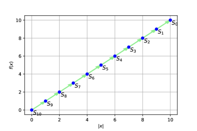
Figure 1: The digraph of the (1+1) EA on OneMax where $n=10$. There is no shortcut.

The second example is the (1+1) EA for maximizing the FullyDeceptive (or called Trap) function:

$$\mathrm{FD}(x)=\left\{\begin{array}[]{lll}n+1&\mbox{if }|x|=0,\\ |x|&\mbox{else}.\end{array}\right.$$ (15)

There is one global maximum $x:|x|=0$ and one local maximum $x:|x|=n$. The state space is split into $n+1$ fitness levels $(S_{0},\cdots,S_{n})$ where $S_{k}=\{x\in\{0,1\}^{n}:\mathrm{FD}(x)=n-k\}$. Figure 2 displays the digraph of the (1+1) EA on FullyDeceptive. FullyDeceptive is the hardest function to the (1+1) EA [23]. The upper time bound is $O(n^{n})$.

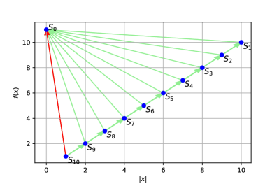
Figure 2: The digraph of the (1+1) EA on FullyDeceptive where $n=10$. The red arc is a weak shortcut.

The third example is the (1+1) EA for maximizing the TwoMax1 function [18]. Let $n$ be a large even integer.

$$\small\mathrm{TM1}(x)=\left\{\begin{array}[]{lll}n&\mbox{if }|x|=0\mbox{ or }|x|=n,\\ |x|&\mbox{if }|x|\geq n/2,\\ n/2-|x|&\mbox{else}.\end{array}\right.$$ (16)

Figure 3 displays the digraph of the (1+1) EA on TwoMax1. There are two maxima at $|x|=0$ and $|x|=n$. The search space is split into $n$ fitness levels $(S_{0},\cdots,S_{n-1})$ where $S_{k}=\{x\in\{0,1\}^{n}:\mathrm{TM1}(x)=n-k\}$. TwoMax1 is as easy as OneMax. The upper time bound is $O(n\ln n)$.

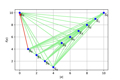
Figure 3: The digraph of the (1+1) EA on TwoPath1 where $n=10$. The red arc is a strong shortcut.

The fourth example is the (1+1) EA for maximizing a deceptive function, named Deceptive:

$$\mathrm{DE}(x)=\left\{\begin{array}[]{lll}n-2|x|&\mbox{if }|x|\leq n/2\\ |x|-n-1&\mbox{else},\end{array}\right.$$ (19)

where $n$ is a large even integer. There are one global maximum at $|x|=0$ and one local optimum at $|x|=n$. The state space is split into $n+1$ fitness levels $(S_{0},\cdots,S_{n})$ where $S_{k}=\{x\in\{0,1\}^{n}:\mathrm{DE}(x)=n-k\}$. Figure 4 shows the digraph of the (1+1) EA on Deceptive. Deceptive is hard to the (1+1) EA. The upper time bound is $O(n^{n})$.

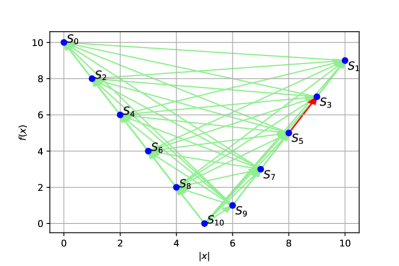
Figure 4: The digraph of the (1+1) EA on Deceptive where $n=10$. The red arc is a strong shortcut.

In all these four examples, for all $k,\ell$, transition probabilities $p_{{\scriptscriptstyle\max}}({x}_{k},S_{\ell})=p_{{\scriptscriptstyle\min}}({x}_{k},S_{\ell})$. Therefore, the best lower bound in Theorem 1 is equal to the best upper bound in Theorem 2. Both are the exact hitting time.

IV-C Shortcuts

There are different paths from a lower fitness level to a higher one, where some paths are shorter than others. A shorter path means that one or more fitness levels are skipped. Shortcuts are widespread in fitness functions with multiple optima. The (weak) shortcut is defined in [18] as follows.

Definition 6

Given an elitist EA for maximizing $f(x)$ and a fitness level partition $(S_{0},\cdots,S_{K})$, there is a (weak) shortcut from $X_{k}\in S_{k}$ to $S_{[0,\ell-1]}$ skipping $S_{\ell}$ (where $k\ >\ell$) if the conditional probability

$$\frac{p(X_{k},S_{\ell})}{p(X_{k},S_{[0,\ell]})}=o(1),$$ (20)

Condition (20) means that the conditional probability of the EA visiting the level $S_{\ell}$ is $o(1)$, but the probability of visiting $S_{[0,\ell-1]}$ is $1-o(1)$. Thus, the level $S_{\ell}$ is skipped with a large probability $1-o(1)$. Figure 4 shows that the (1+1) EA on FullyDeceptive takes a weak shortcut $S_{n}\to S_{0}$ skipping $S_{1}$. According to [18, Theorem 7], a shortcut results in small coefficients $c$ and $c_{\ell}$. Hence, Type-$c$ and $c_{\ell}$ lower bounds are not tight for EAs on fitness landscapes with weak shortcuts.

In this paper, shortcuts refer to (strong) shortcuts, which are defined as follows.

Definition 7

Given an elitist EA for maximizing $f(x)$ and a fitness level partition $(S_{0},\cdots,S_{K})$, there is a (strong) shortcut from $X_{k}\in S_{k}$ to $S_{[0,\ell-1]}$ skipping $S_{[\ell,k-1]}$ (where $k\ >\ell$) if the conditional probability $r(X_{k},S_{[\ell,k-1]})=o(1)$, that is

$$\frac{p(X_{k},S_{[\ell,k-1]})}{p(X_{k},S_{[0,k]})}=o(1).$$ (21)

Condition (21) requires skipping all levels from $S_{\ell}$ to $S_{k-1}$, but (20) only requires skipping one level $S_{\ell}$. For example, in Figure 4, the path $S_{n}\to S_{0}$ is a weak shortcut skipping $S_{1}$ because $r(x_{n},S_{1})=o(1)$, but not a strong shortcut because $r(x_{n},S_{[1,n-1]})$ is $\Omega(1)$. Figure 3 shows that the (1+1) EA on TwoMax1 takes a strong shortcut $S_{n/2+1}\to S_{0}$ skipping $S_{1}$ because $r(x_{n/2+1},S_{[1,n/2]})=o(1)$. Figure 4 shows that the (1+1) EA on Deceptive takes a strong shortcut $S_{5}\to S_{3}$ skipping $S_{4}$ because $r(x_{5},S_{4})=o(1)$. In summary,

• OneMax: one global optimum. There is no shortcut.

• FullyDeceptive: One global optimum and one local optimum. Weak shortcuts exist but no strong shortcut.

• TwoMax1: Two global optima. Strong shortcuts exist.

• Deceptive: One global optimum and one local optimum. Strong shortcuts exist.

IV-D Sub-digraphs

Let $S^{\prime}$ be a subset of non-optimal states and $S^{\prime}_{\mathrm{opt}}=S\setminus S^{\prime}$. A new absorbing Markov chain can be constructed whose transition probabilities satisfy

$$p^{\prime}(X,Y)=\left\{\begin{array}[]{ll}p(X,Y)&\mbox{if }X\in S^{\prime},\\ 0&\mbox{if }X\in S^{\prime}_{\mathrm{opt}},Y\notin S^{\prime}_{\mathrm{opt}}.\end{array}\right.$$ (22)

For states in the subset $S^{\prime}$, their transition probabilities (22) are the same as the original ones (5). For the new chain, its hitting time is modified to be the number of generations for the EA to hit $S^{\prime}_{\mathrm{opt}}$ for the first time.

Definition 8

The (random) hitting time for an EA starting from $X^{[0]}=X$ to hit $S^{\prime}_{\mathrm{opt}}$ is

$$\tau^{\prime}(X)=\min\{t\geq 0,X^{[t]}\in S^{\prime}_{\mathrm{opt}}\mid X^{[0]}=X\}.$$ (23)

The mean hitting time $m^{\prime}(X)=\mathrm{E}[\tau^{\prime}(X)].$

Lemma 1

The hitting time $m^{\prime}(X)\leq m(X)$.

Proof:

Since $S_{\mathrm{opt}}\subset S^{\prime}_{\mathrm{opt}}$, the mean time to hit $S^{\prime}_{\mathrm{opt}}$ is less than the mean time to hit $S_{\mathrm{opt}}$. ∎

Definition 9

A subset $S^{\prime}$ of non-optimal states is split into $K$ ranks according to the fitness value from high to low, denoted by $(S^{\prime}_{1},\cdots,S^{\prime}_{K})$. Let $S^{\prime}_{0}=S^{\prime}_{\mathrm{opt}}$ include the remaining states. $(S^{\prime}_{0},S^{\prime}_{1},\cdots,S^{\prime}_{K})$ is called a level partition.

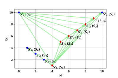
Figure 5: A sub-digraph of the (1+1) EA on TwoMax1 where $n=10$. Original fitness levels $(S_{1},S_{2},S_{3},S_{4},S_{5},S_{9})$ are relabeled as levels $(S^{\prime}_{1},S^{\prime}_{2},S^{\prime}_{3},S^{\prime}_{4},S^{\prime}_{5},S^{\prime}_{6})$. There is no transition from $S^{\prime}_{0}$ to $S_{k}$ where $k\geq 1.$

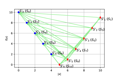
Figure 6: A sub-digraph of the (1+1) EA on Deceptive where $n=10$. Original fitness levels $(S_{2},S_{4},S_{6},S_{8},S_{9})$ are relabeled as levels $(S^{\prime}_{1},S^{\prime}_{2},S^{\prime}_{3},S^{\prime}_{4},S^{\prime}_{5})$. There is no transition from $S^{\prime}_{0}$ to $S_{k}$ where $k\geq 1.$

Different from $S_{0}$ in a fitness level partition, $S^{\prime}_{0}$ includes some non-optimal fitness levels. This difference can be observed from Figure 3 vs Figure 5 or Figure 4 vs Figure 6.

Definition 10

The behavior of an elitist EA on a sub-digraph can be represented by a Markov chain on a sub-digraph $G^{\prime}=(V^{\prime},A^{\prime})$ where

• $V^{\prime}$ denotes the set of vertexes where a vertex $k$ represents a fitness level $S^{\prime}_{k},\ k=1,\cdots,K$. The vertex $0$ represents the remaining fitness levels.

• $A^{\prime}$ denotes the set of arcs where an arc $(k,l)$ represents the transition from $S_{k}$ to $S_{\ell}$ (where $k>\ell$) with $p_{{\scriptscriptstyle\min}}(X_{k},S^{\prime}_{\ell})>0$.

Corollary 1 is the sub-digraph version of Theorem 1, with the same proof argument.

Corollary 1

For an elitist EA that maximizes $f(x)$, given a level partition $(S^{\prime}_{0},\cdots,S^{\prime}_{K})$, for $k\geq 1$, $d^{\prime}_{k}$ is constructed as follows

$$d^{\prime}_{k}=\frac{1}{p_{{\scriptscriptstyle\max}}(X_{k},S^{\prime}_{[0,k-1]})}+\sum^{k-1}_{\ell=1}\frac{c^{\prime}_{k,\ell}}{p_{{\scriptscriptstyle\max}}(X_{\ell},S^{\prime}_{[0,\ell-1]})},$$ (24)

where the coefficient $c^{\prime}_{k,\ell}\in[0,1]$ satisfies

$$c^{\prime}_{k,\ell}\leq r_{{\scriptscriptstyle\min}}(X_{k},S^{\prime}_{\ell})+\sum^{k-1}_{j=\ell+1}{r}_{{\scriptscriptstyle\min}}(X_{k},S^{\prime}_{j})c_{j,\ell}.$$ (25)

Then the mean hitting time $m^{\prime}(X_{k})\geq d^{\prime}_{k}.$

V The Digraph Method for Linear Bounds

This section presents a fast non-recursive method to calculate coefficients based on digraphs.

V-A Calculation of Coefficients in the Lower Bound

For an elitist EA that maximizes $f(x)$, given a fitness level partition (or a level partition) $(S_{0},S_{1},\cdots,S_{K})$, the linear lower bound is

$$d_{k}=\frac{1}{p_{{\scriptscriptstyle\max}}(X_{k},S_{[0,k-1]})}+\sum^{k-1}_{\ell=1}\frac{c_{k,\ell}}{p_{{\scriptscriptstyle\max}}(X_{\ell},S_{[0,\ell-1]})},$$

From (10), by induction, it is straightforward to obtain an explicit expression for $c_{k,\ell}$ as follows:

$$\begin{split}c_{k,\ell}&\leq r_{{\scriptscriptstyle\min}}(X_{k},S_{\ell})+\sum_{\ell<k_{1}<k}r_{{\scriptscriptstyle\min}}(X_{k},S_{k_{1}})r_{{\scriptscriptstyle\min}}(X_{k_{1}},S_{\ell})\\ &+\sum_{\ell<k_{2}<k_{1}<k}r_{{\scriptscriptstyle\min}}(X_{k},S_{k_{1}})r_{{\scriptscriptstyle\min}}(X_{k_{1}},S_{k_{2}})r_{{\scriptscriptstyle\min}}(X_{k_{2}},S_{\ell})\\ &+\cdots\cdots\\ =&\sum_{\mathrm{path}[k,\ell]\in\mathrm{PATH}[k,\ell]}\prod_{(k_{j},k_{j+1})\in\mathrm{path}[k,\ell]}r_{{\scriptscriptstyle\min}}(X_{k_{j}},S_{k_{j+1}}).\end{split}$$

But the above calculation is intractable because the number of paths is $O((k-\ell-1)!)$. Therefore, $c_{k,\ell}$ needs to be computed quickly in polynomial time.

To calculate the coefficient $c_{k,\ell}$, we consider the full path from $k$ to $\ell$: $S_{k}\to S_{k-1}\to\cdots\to S_{\ell+1}\to S_{\ell}.$ Using the conditional probabilities $r_{{\scriptscriptstyle\min}}(X_{i},S_{[\ell,i-1]})$ for each vertex $i>\ell$ on the path, we can calculate the coefficient $c_{k,l}$ and derive the following lower bound.

Theorem 3

For an elitist EA that maximizes $f(x)$, given a fitness level partition or a level partition $(S_{0},S_{1},\cdots,S_{K})$, for $k\geq 1$, $d_{k}$ is constructed as follows

$$d_{k}=\frac{1}{p_{{\scriptscriptstyle\max}}(X_{k},S_{[0,k-1]})}+\sum^{k-1}_{\ell=1}\frac{c_{k,\ell}}{p_{{\scriptscriptstyle\max}}(X_{\ell},S_{[0,\ell-1]})},$$ (26)

where the coefficient $c_{k,\ell}\in[0,1]$ satisfies

$$c_{k,l}\leq\prod^{k}_{i=\ell+1}r_{{\scriptscriptstyle\min}}(X_{i},S_{[\ell,i-1]}).$$ (27)

Then $m(X_{k})\geq d_{k}$.

Proof:

Without loss of generality, we only consider a fitness level partition $(S_{0},\cdots,S_{K})$ and apply Theorem 1 in the proof. For a level partition $(S_{0},\cdots,S_{K})$, Corollary 1 is applied in the proof.

Let $c^{*}_{k,\ell}$ (where $k>\ell$) denote the best (largest) coefficient in (10) in Theorem 1. It is sufficient to prove by induction that $c^{*}_{k,\ell}$ is larger than the best coefficient from (27), that is.

$$c^{*}_{k,\ell}\geq\prod^{k}_{i=\ell+1}r_{{\scriptscriptstyle\min}}(X_{i},S_{[\ell,i-1]}).$$ (28)

For $\ell+1$, it is trivial that $c^{*}_{\ell+1,\ell}=r_{{\scriptscriptstyle\min}}(X_{\ell+1},S_{\ell}).$ For $\ell+2$, we have

$$c^{*}_{\ell+2,\ell} =r_{{\scriptscriptstyle\min}}(X_{\ell+2},S_{\ell})+r_{{\scriptscriptstyle\min}}(X_{\ell+2},S_{\ell+1})c^{*}_{\ell+1,\ell}$$

$$=r_{{\scriptscriptstyle\min}}(X_{\ell+2},S_{\ell})+r_{{\scriptscriptstyle\min}}(X_{\ell+2},S_{\ell+1})r_{{\scriptscriptstyle\min}}(X_{\ell+1},S_{\ell})$$

$$\geq\left(r_{{\scriptscriptstyle\min}}(X_{\ell+2},S_{\ell})+r_{{\scriptscriptstyle\min}}(X_{\ell+2},S_{\ell+1})\right)r_{{\scriptscriptstyle\min}}(X_{\ell+1},S_{\ell})$$

$$\geq r_{{\scriptscriptstyle\min}}(X_{\ell+2},S_{[\ell,\ell+1]})r_{{\scriptscriptstyle\min}}(X_{\ell+1},S_{\ell}).$$

Suppose that (28) holds for $\ell+1,\cdots,\eta-1$. We prove that (28) holds for $k=\eta$.

$$\small\begin{split}&c^{*}_{\eta,\ell}=r_{{\scriptscriptstyle\min}}(X_{\eta},S_{\ell})+\sum^{\eta-1}_{j=\ell+1}{r}_{{\scriptscriptstyle\min}}(X_{\eta},S_{j})c^{*}_{j,\ell}\\ &\geq r_{{\scriptscriptstyle\min}}(X_{\eta},S_{\ell})+\sum^{\eta-1}_{j=\ell+1}{r}_{{\scriptscriptstyle\min}}(X_{\eta},S_{j})\prod^{j}_{i=\ell+1}r_{{\scriptscriptstyle\min}}(X_{i},S_{[\ell,i-1]})\\ &\geq r_{{\scriptscriptstyle\min}}(X_{\eta},S_{\ell})+\sum^{\eta-1}_{j=\ell+1}{r}_{{\scriptscriptstyle\min}}(X_{\eta},S_{j})\prod^{\eta-1}_{i=\ell+1}r_{{\scriptscriptstyle\min}}(X_{i},S_{[\ell,i-1]})\\ &=r_{{\scriptscriptstyle\min}}(X_{\eta},S_{\ell})+{r}_{{\scriptscriptstyle\min}}(X_{\eta},S_{[\ell+1,\eta-1]})\prod^{\eta-1}_{i=\ell+1}r_{{\scriptscriptstyle\min}}(X_{i},S_{[\ell,i-1]})\\ &\geq\left(r_{{\scriptscriptstyle\min}}(X_{k},S_{\ell})+r_{{\scriptscriptstyle\min}}(X_{\eta},S_{[\ell+1,\eta-1]})\right)\prod^{\eta-1}_{i=\ell+1}r_{{\scriptscriptstyle\min}}(X_{i},S_{[\ell,i-1]})\\ &=\prod^{\eta}_{i=\ell+1}r_{{\scriptscriptstyle\min}}(X_{i},S_{[\ell,i-1]}).\end{split}$$

Thus by induction, for any $k>\ell$, (28) holds. Then we have for any $k\geq 1$, $d(X_{k})\leq d^{*}(X_{k})\leq m(X_{k})$. ∎

The conditional transition probability $r_{{\scriptscriptstyle\min}}(X_{i},S_{[\ell,i-1]})$ can be calculated from two transition probabilities.

Corollary 2

The coefficients in Theorem 3 can be set to be

$$c_{k,l}\leq\prod^{k}_{i=\ell+1}\frac{1}{1+\frac{p_{{\scriptscriptstyle\max}}(X_{i},S_{[0,\ell-1]})}{p_{{\scriptscriptstyle\min}}(X_{i},S_{[\ell,i-1]})}}.$$ (29)

Proof:

Since the conditional probability

$$r_{{\scriptscriptstyle\min}}(X_{i},S_{[\ell,i-1]})=\min_{X_{i}\in S_{i}}\frac{p(X_{i},S_{[\ell,i-1]})}{p(X_{i},S_{[0,i-1]})}$$

$$= \min_{X_{i}\in S_{i}}\frac{p(X_{i},S_{[\ell,i-1]})}{p(X_{i},S_{[0,\ell-1]})+p(X_{i},S_{[\ell,i-1]})}$$

$$= \min_{X_{i}\in S_{i}}\frac{1}{1+\frac{p(X_{i},S_{[0,\ell-1]})}{p(X_{i},S_{[\ell,i-1]})}}\geq\frac{1}{1+\frac{\max_{X_{i}}p(X_{i},S_{[0,\ell-1]})}{\min_{X_{i}}p(X_{i},S_{[\ell,i-1]})}}$$

$$=\frac{1}{1+\frac{p_{{\scriptscriptstyle\max}}(X_{i},S_{[0,\ell-1]})}{p_{{\scriptscriptstyle\min}}(X_{i},S_{[\ell,i-1]})}},$$

we obtain the required conclusion from Theorem 3. ∎

In Corollary 2, the transition probability $p(X_{i},S_{[0,i-1]})$ from the level $i$ to the higher levels $S_{[0,i-1]}$ is divided into two parts: (i) $p(X_{i},S_{[0,\ell-1]})$ for the transition beyond the level $\ell$ and (ii) $p(X_{i},S_{[\ell,i-1]})$ for the transition up to the level $\ell$. The ratio between them determines the coefficient $c_{k,\ell}$. Both probabilities are easy to calculate because $S_{[0,\ell-1]}$ and $S_{[\ell,i-1]}$ represent consecutive fitness levels.

V-B Calculation of Coefficients in the Upper Bound

Likewise, Theorem 4 provides a fast calculation of coefficients in the linear upper bound. It applies only for the setting of a given fitness level partition, not for a level partition.

Theorem 4

For an elitist EA that maximizes $f(x)$, given a fitness level partition $(S_{0},S_{1},\cdots,S_{K})$, for $k\geq 1$, $d_{k}$ is constructed as follows

$$d_{k}=\frac{1}{p_{{\scriptscriptstyle\min}}(X_{k},S_{[0,k-1]})}+\sum^{k-1}_{\ell=1}\frac{c_{k,\ell}}{p_{{\scriptscriptstyle\min}}(X_{\ell},S_{[0,\ell-1]})},$$ (30)

where the coefficient $c_{k,\ell}\in[0,1]$ satisfies

$$c_{k,l}\geq r_{{\scriptscriptstyle\max}}(X_{k},S_{[\ell,k-1]}).$$ (31)

Then $m(X_{k})\leq d_{k}$.

Proof:

According to Theorem 2, we have for any $1\leq\ell<k\leq K$,

$$c_{k,\ell}\geq r_{{\scriptscriptstyle\max}}(X_{k},S_{\ell})+\sum^{k-1}_{j=\ell+1}{r}_{{\scriptscriptstyle\max}}(X_{k},S_{j})c_{j,\ell}.$$ (32)

Let $c_{j,\ell}=1$ on the right-hand side. Then we get the required conclusion. ∎

The conditional transition probability $r_{{\scriptscriptstyle\max}}(X_{i},S_{[\ell,i-1]})$ can be calculated from two transition probabilities. The proof of Corollary 3 is similar to that of Corollary 2.

Corollary 3

The coefficients in Theorem 4 can be set to be

$$c_{k,l}\geq\frac{1}{1+\frac{p_{{\scriptscriptstyle\min}}(X_{k},S_{[0,\ell-1]})}{p_{{\scriptscriptstyle\max}}(X_{k},S_{[\ell,k-1]})}}.$$ (33)

V-C Strong Shortcuts and Small Coefficients in the Lower Bound

For a linear lower bound, the larger the coefficients, the tighter the lower bound. According to (27), in order to obtain a coefficient $c_{k,\ell}$ as large as $\Omega(1)$, it is required that most conditional transition probabilities $r_{{\scriptscriptstyle\min}}(X_{i},S_{[\ell,i-1]})$ in (27) are large like $1-1/K$. This is so that the product (27) is a positive constant like $(1-1/K)^{k-\ell}\geq e^{-1}$. However, this requirement is not met if there is a strong shortcut.

Lemma 2

Given an elitist EA for maximizing $f(x)$ and a fitness level partition $(S_{0},\cdots,S_{K})$, if a strong shortcut appears, that is for some vertex $j$ (where $\ell<j\leq k$), the conditional transition probability $r_{{\scriptscriptstyle\min}}(X_{j},S_{[\ell,j-1]})=o(1)$, then the coefficient $c_{k,\ell}=o(1)$ in (27).

Proof:

Since $r_{{\scriptscriptstyle\min}}(X_{j},S_{[\ell,j-1]})=o(1)$, we have

$$\prod^{k}_{i=\ell+1}r_{{\scriptscriptstyle\min}}(X_{i},S_{[\ell,i-1]})=o(1).$$ (34)

According to (27), we obtain $c_{k,l}=o(1)$. ∎

Take the (1+1) EA on TwoMax1 as an example. Assume that the EA starts at $S_{n-1}$. For ease of analysis, consider the coefficient $c_{n-1,1}$ only. According to (27), we assign

$$c_{n-1,1}=\prod^{n-1}_{i=2}r_{{\scriptscriptstyle\min}}(X_{i},S_{[1,i-1]}).$$ (35)

As shown in Figure 3, the EA takes a shortcut $S_{n/2+1}\to S_{0}$ skipping $S_{[1,n/2]}$ with a large probability. We can prove $r(x_{n/2+1},S_{[1,n/2]})=o(1)$. Since $x_{n/2+1}$ has $n-1$ zero-valued bits and $x\in S_{[1,n/2]}$ has at most $n/2$ zero-valued bits, the transition from $x_{n/2+1}$ to $S_{[1,n/2]}$ happens only if at least $n/2-1$ zero-value bits are flipped.

$$p({x}_{n/2+1},S_{[1,n/2]})\leq\binom{n-1}{n/2-1}\left(\frac{1}{n}\right)^{n/2-1}.$$

The transition from $x_{n/2+1}$ to $S_{[0,n/2]}$ happens if $1$ zero-valued bit is flipped and other bits are unchanged. Thus

$$p({x}_{n/2+1},S_{[0,n/2]})\geq\frac{1}{n}\left(1-\frac{1}{n}\right)^{n-1}.$$

We obtain

$$\begin{split}&r_{{\scriptscriptstyle\min}}(x_{n/2+1},S_{[1,n/2]})\leq\frac{p({x}_{n/2+1},S_{[1,n/2]})}{p({x}_{n/2+1},S_{[0,n/2]})}\\ \leq&\frac{\binom{n-1}{n/2-1}\left(\frac{1}{n}\right)^{n/2-1}}{\frac{1}{n}\left(1-\frac{1}{n}\right)^{n-1}}=O\left(\frac{1}{(n/2-1)!}\right).\end{split}$$

Then from (35), we get a small coefficient $c_{n-1,1}=o(1)$.

To avoid this problem, we can consider the subset $S^{\prime}=\{S_{1},S_{2},\cdots,S_{n/2},S_{n-1}\}$ (relabeled by $\{S^{\prime}_{1},\cdots,S^{\prime}_{n/2+1}\}$), then calculate the coefficient $c^{\prime}_{n/2+1,1}$ using a new full path:

$$S^{\prime}_{n/2+1}\to S^{\prime}_{n/2}\to S^{\prime}_{n/2-1}\to\cdots\to S^{\prime}_{2}\to S^{\prime}_{1}.$$

A detailed analysis is given in Section VI-D.

The general usage of Theorem 3 and Corollary 2 is summarized as follows: (i) digraph versions are suitable for fitness functions without shortcuts or with weak shortcuts, e.g., OneMax and FullyDeceptive, (ii) sub-digraph version are used for fitness functions with strong shortcuts, e.g., TwoMax1 and Deceptive. The choice of a sub-digraph is flexible. A good choice is to select a non-optimal subset $S^{\prime}$ such that for the full path $S^{\prime}_{K}\to\cdots\to S^{\prime}_{0}$ of the corresponding sub-digraph, for all arcs $(i,i-1)$ on the path, the conditional transition probability $r_{{\scriptscriptstyle\min}}(X^{\prime}_{i},S^{\prime}_{i-1})$ from $S^{\prime}_{i}$ to $S^{\prime}_{i-1}$ is as large as $\Omega(1)$. For example, a good choice for the (1+1) EA on TwoMax1 is $S^{\prime}=\{S_{1},S_{2},\cdots,S_{n/2},S_{n-1}\}$ (Figure 5). For the (1+1) EA on Deceptive, a good choice is $S^{\prime}=\{S_{1},S_{3},\cdots,S_{n-3},S_{n-1},S_{n}\}$ (Figure 6).

VI Examples

This section demonstrates that the digraph method is easy and quick to estimate linear bounds through examples.

VI-A The Upper Bound of the (1+1) EA on OneMax

Consider the (1+1) EA that maximizes OneMax. Assume that the EA starts at $S_{n}$. We estimate the linear upper bound

$$d_{n}=\frac{1}{p_{\scriptscriptstyle\min}({x}_{n},S_{[0,n-1]})}+\sum^{n-1}_{\ell=1}\frac{c_{n,\ell}}{p_{\scriptscriptstyle\min}({x}_{\ell},S_{[0,\ell-1]})}.$$

The coefficient $c_{n,\ell}$ (where $1\leq\ell<n$) is calculated by (33). Since $x_{n}\in S_{n}$ has $n$ zero-valued bits, the transition from $x_{n}$ to $S_{[0,\ell-1]}$ happens if at least $n-\ell+1$ zero-valued bits are flipped and other bits are unchanged, equivalently, if one of the following events happens: $j$ (where $j=n-\ell+1,\cdots,n$) zero-valued bits are flipped, and other bits are unchanged. The transition probability

$$p_{\scriptscriptstyle\min}(x_{n},S_{[0,\ell-1]}) \geq\sum^{n}_{j=n-l+1}\binom{n}{j}\left(\frac{1}{n}\right)^{j}\left(1-\frac{1}{n}\right)^{n-j}.$$

The transition from $x_{n}$ to $S_{[\ell,n-1]}$ happens only if one of the following events happens: $j$ zero-valued (where $1\leq j\leq n-\ell$) bits are flipped and other $n-j$ zero-valued bits are unchanged. The transition probability

$$p_{\scriptscriptstyle\max}(x_{n},S_{[\ell,n-1]})\leq\sum^{n-\ell}_{j=1}\binom{n}{j}\left(\frac{1}{n}\right)^{j}\left(1-\frac{1}{n}\right)^{n-j}.$$

According to (33), we assign the coefficient

$$c_{n,\ell}=\frac{1}{1+\frac{\sum^{n}_{j=n-l+1}\binom{n}{j}\left(\frac{1}{n}\right)^{j}\left(1-\frac{1}{n}\right)^{n-j}}{\sum^{n-\ell}_{j=1}\binom{n}{j}\left(\frac{1}{n}\right)^{j}\left(1-\frac{1}{n}\right)^{n-j}}}=O(1).$$ (36)

Figure 7 illustrates the coefficient $c_{200,\ell}$ in (36) when $n=200$.

The transition probability $p({x}_{\ell},S_{[0,\ell-1]})$ (where $\ell\geq 1$) is calculated as follows. Since $x_{\ell}\in S_{\ell}$ has $\ell$ zero-valued bits, the transition from $x_{\ell}$ to $S_{[0,\ell-1]}$ happens if one of the following events happens: $j$ (where $j=1,\cdots,\ell$) zero-valued bits are flipped and other bits are not flipped. The transition probability

$$\small\begin{split}p_{\scriptscriptstyle\min}({x}_{\ell},S_{[0,\ell-1]})&\geq\sum^{\ell}_{j=1}\binom{\ell}{j}\left(\frac{1}{n}\right)^{j}\left(1-\frac{1}{n}\right)^{n-j}=\Omega\left(\frac{\ell}{en}\right).\end{split}$$

Finally, we obtain the linear upper bound

$$d_{n}\leq 1+\sum^{n-1}_{\ell=1}O(1)O\left(\frac{en}{\ell}\right)=O(n\ln n).$$

VI-B The Lower Bound of the (1+1) EA on OneMax

Consider the (1+1) EA that maximizes OneMax. Assume that the EA starts at $S_{n}$. We estimate the lower bound,

$$d_{n}=\frac{1}{p_{{\scriptscriptstyle\max}}({x}_{n},S_{[0,n-1]})}+\sum^{n-1}_{\ell=1}\frac{c_{n,\ell}}{p_{{\scriptscriptstyle\max}}({x}_{\ell},S_{[0,\ell-1]})}.$$

The coefficient $c_{n,\ell}$ (where $1\leq\ell<n$) for the lower bound is calculated by (27). For $\ell<i\leq n$, $x_{i}\in S_{i}$ has $i$ zero-valued bits. The transition from $x_{i}$ to $S_{[0,\ell-1]}$ happens only if one of the following events happens: $j$ (where $j=i-\ell+1,\cdots,i$) zero-valued bits are flipped and $i-j$ zero-valued bits are not flipped.The transition probability

$$p_{{\scriptscriptstyle\max}}({x}_{i},S_{[0,\ell-1]})\leq \sum^{i}_{j=i-l+1}\binom{i}{j}\left(\frac{1}{n}\right)^{j}\left(1-\frac{1}{n}\right)^{i-j}.$$

The transition from $x_{i}$ to $S_{[\ell,i-1]}$ happens if $j$ zero-value (where $1\leq j\leq i-\ell$) bits are flipped and other bits are unchanged. The transition probability

$$p_{{\scriptscriptstyle\min}}({x}_{i},S_{[\ell,i-1]})\geq\sum^{i-\ell}_{j=1}\binom{i}{j}\left(\frac{1}{n}\right)^{j}\left(1-\frac{1}{n}\right)^{n-j}.$$

According to (29), we assign the coefficient

$$c_{n,\ell}=\prod^{n}_{i=\ell+1}\frac{1}{1+\frac{\sum^{i}_{j=i-l+1}\binom{i}{j}\left(\frac{1}{n}\right)^{j}\left(1-\frac{1}{n}\right)^{i-j}}{\sum^{i-\ell}_{j=1}\binom{i}{j}\left(\frac{1}{n}\right)^{j}\left(1-\frac{1}{n}\right)^{n-j}}}.$$ (37)

Then we prove

$$c_{n,l}=\Omega(1).$$ (38)

The proof of (38) is given in the Appendix. Figure 7 illustrates the lower bound coefficient $c_{200,\ell}$ in (37) when $n=200$. Its value decreases from 1.0 to around 0.5. There is an increase in value from $c_{200,198}$ to $c_{200,199}$. This phenomenon is caused by (27). According to (27), $c_{n,n-1}=r_{{\scriptscriptstyle\min}}(x_{n},S_{n-1})$ is a single conditional transition probability, but $c_{n,n-2}=r_{{\scriptscriptstyle\min}}(x_{n},S_{[n-2,n-1]})\times r_{{\scriptscriptstyle\min}}(x_{n-1},S_{n-2})$ is a product of two conditional probabilities. The former is larger than the latter. It can be seen from Figure 7 that the lower bound coefficient is at least 1/2 of the upper bound coefficient.

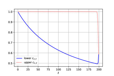
Figure 7: Coefficients $c_{200,\ell}$ (where $\ell=1,\cdots,199$) in linear lower and upper bounds of the (1+1) EA on OneMax where $n=200$.

The transition probability $p({x}_{\ell},S_{[0,\ell-1]})$ (where $\ell\geq 1$) is calculated as follows. Since $x_{\ell}\in S_{\ell}$ has $\ell$ zero-valued bits, the transition from $x_{\ell}$ to $S_{[0,\ell-1]}$ happens only if at least 1 zero-valued bit is flipped, or more accurately, only if one of the following events happens: $j$ (where $j=1,\cdots,\ell$) zero-valued bits are flipped and $i-j$ zero-valued bits are not flipped. The transition probability

$$p_{{\scriptscriptstyle\max}}({x}_{\ell},S_{[0,\ell-1]}) \leq\sum^{\ell}_{j=1}\binom{\ell}{j}\left(\frac{1}{n}\right)^{j}\left(1-\frac{1}{n}\right)^{\ell-j}\leq\frac{\ell}{n}.$$

Finally, we obtain the linear lower bound

$$d_{n}\geq 1+\sum^{n-1}_{\ell=1}\Omega(1)\frac{n}{\ell}=\Omega(n\ln n).$$

The lower bound is tight because the upper bound is $O(n\ln n)$.

VI-C The Lower Bound of the (1+1) EA on FullyDeceptive

Consider the (1+1) EA that maximizes FullyDeceptive. Assume that the EA starts at $S_{n}$. We estimate the lower bound

$$d_{n}=\frac{1}{p_{{\scriptscriptstyle\max}}({x}_{n},S_{[0,n-1]})}+\sum^{n-1}_{\ell=1}\frac{c_{n,\ell}}{p_{{\scriptscriptstyle\max}}({x}_{\ell},S_{[0,\ell-1]})}.$$

The coefficient $c_{n,\ell}$ (where $1\leq\ell<n$) is calculated by (27). For $\ell<i\leq n$, $x_{i}$ has $i-1$ zero-valued bits, the transition from $x_{i}$ to $S_{[0,\ell-1]}$ happens only if (i) at least $i-\ell+1$ zero-valued bits are flipped to enter $S^{\prime}_{[1,\ell-1]}$, or (ii) it is mutated to $(0,\cdots,0)$. The transition probability

$$\begin{split}p_{{\scriptscriptstyle\max}}({x}_{i},S_{[0,\ell-1]})\leq&\binom{i-1}{i-\ell+1}\left(\frac{1}{n}\right)^{i-\ell+1}\\ &+\left(\frac{1}{n}\right)^{n-i+1}\left(1-\frac{1}{n}\right)^{i-1}.\end{split}$$

The transition from $x_{i}$ to $S_{[\ell,i-1]}$ happens if $j$ zero-value bits (where $1\leq j\leq i-\ell$) are flipped and other bits are unchanged. The transition probability

$$p_{{\scriptscriptstyle\min}}({x}_{i},S_{[\ell,i-1]})\geq\sum^{i-\ell}_{j=1}\binom{i-1}{j}\left(\frac{1}{n}\right)^{j}\left(1-\frac{1}{n}\right)^{n-j}.$$

According to (29), we assign the coefficient

$$\begin{split}c_{n,\ell}=\prod^{n}_{i=\ell+1}\frac{1}{1+\frac{\binom{i-1}{i-\ell+1}\left(\frac{1}{n}\right)^{i-\ell+1}+\left(\frac{1}{n}\right)^{n-i+1}\left(1-\frac{1}{n}\right)^{i-1}}{\sum^{i-\ell}_{j=1}\binom{i-1}{j}\left(\frac{1}{n}\right)^{j}\left(1-\frac{1}{n}\right)^{n-j}}}.\end{split}$$

Then we prove

$$c_{n,\ell}=\Omega(1).$$ (39)

The proof of (39) is given in the Appendix.

The transition probability $p({x}_{\ell},S_{[0,\ell-1]})$ (where $\ell\geq 1$) is calculated as follows. Since $x_{1}\in S_{1}$ has $n$ one-valued bits, the transition from $x_{1}$ to $S_{0}$ happens if only if all bits are flipped. Obviously, the transition probability

$$p_{{\scriptscriptstyle\max}}({x}_{1},S_{0})=n^{-n}.$$

For $\ell\geq 2$, since $x_{\ell}\in S_{\ell}$ has $\ell-1$ zero-valued bits, the transition from $x_{\ell}$ to $S_{[0,\ell-1]}$ happens only if (i) at least 1 zero-valued bit is flipped, or (ii) $x_{\ell}$ is mutated to $(0,\cdots,0)$. The transition probability

$$p_{{\scriptscriptstyle\max}}({x}_{\ell},S_{[0,\ell-1]})\leq\frac{\ell-1}{n}+\left(\frac{1}{n}\right)^{n-\ell+1}\leq\frac{\ell}{n}.$$

Finally, we get a lower bound as

$$d_{n}\geq 1+\Omega(1)n^{n}+\sum^{n-1}_{\ell=2}\Omega(1)\frac{n}{\ell}=\Omega(n^{n}).$$

The lower bound is tight because the upper bound is $O(n^{n})$.

VI-D The Lower Bound of the (1+1) EA on TwoMax1

Consider the (1+1) EA on TwoMax1. We construct a level partition as follows (Figure 5): let $S^{\prime}_{\ell}=S_{\ell}$ for $\ell=1,\cdots,n/2$, $S^{\prime}_{n/2+1}=S_{n-1}$, and $S^{\prime}_{0}$ represent the set of all remaining fitness levels. Let $x^{\prime}_{k}$ denote a state in $S^{\prime}_{k}$. Assume that the EA starts at $S^{\prime}_{n/2+1}$. We estimate the lower bound

$$d^{\prime}_{n/2+1}=\frac{1}{p_{{\scriptscriptstyle\max}}({x}_{n/2+1},S^{\prime}_{[0,n/2]})}+\sum^{n/2}_{\ell=1}\frac{c^{\prime}_{n/2+1,\ell}}{p_{{\scriptscriptstyle\max}}({x}_{\ell},S^{\prime}_{[0,\ell-1]})}.$$

The coefficient $c^{\prime}_{n/2+1,\ell}$ (where $1\leq\ell\leq n/2$) is calculated by (29). It is trivial that

$$p_{{\scriptscriptstyle\max}}({x}^{\prime}_{n/2+1},S^{\prime}_{[0,\ell-1]})\leq 1.$$

The transition from $x^{\prime}_{n/2+1}$ to $S^{\prime}_{[0,\ell-1]}$ happens if one bit is flipped. The transition probability

$$p_{{\scriptscriptstyle\min}}({x}^{\prime}_{n/2+1},S^{\prime}_{[\ell,n/2]})\geq\binom{n}{1}\frac{1}{n}\left(1-\frac{1}{n}\right)^{n-1}\geq e^{-1}.$$

For $\ell<i\leq n/2$, $x^{\prime}_{i}$ has $i$ zero-valued bits. The transition from $x^{\prime}_{i}$ to $S^{\prime}_{[0,\ell-1]}$ happens only if (i) at least $i-\ell+1$ zero-valued bits are flipped to enter $S^{\prime}_{[0,\ell-1]}$, or (ii) it is mutated to $(0,\cdots,0)$. The transition probability

$$\footnotesize\begin{split}p_{{\scriptscriptstyle\max}}({x}^{\prime}_{i},S^{\prime}_{[0,\ell-1]})\leq\binom{i}{i-\ell+1}\left(\frac{1}{n}\right)^{i-\ell+1}+\left(\frac{1}{n}\right)^{n-i}\left(1-\frac{1}{n}\right)^{i}.\end{split}$$

The transition from $x^{\prime}_{i}$ to $S^{\prime}_{[\ell,i-1]}$ happens if $j$ zero-value bits (where $1\leq j\leq i-\ell$) are flipped and other bits are unchanged. The transition probability

$$p_{{\scriptscriptstyle\min}}({x}^{\prime}_{i},S^{\prime}_{[\ell,i-1]})\geq\sum^{i-\ell}_{j=1}\binom{i}{j}\left(\frac{1}{n}\right)^{j}\left(1-\frac{1}{n}\right)^{n-j}.$$

According to (29), we assign

$$\begin{split}c^{\prime}_{n/2+1,\ell}=\frac{1}{1+e}\prod^{n/2}_{i=\ell}\frac{1}{1+\frac{\binom{i}{i-\ell+1}\left(\frac{1}{n}\right)^{i-\ell+1}+\left(\frac{1}{n}\right)^{n-i}\left(1-\frac{1}{n}\right)^{i}}{\sum^{i-\ell}_{j=1}\binom{i}{j}\left(\frac{1}{n}\right)^{j}\left(1-\frac{1}{n}\right)^{n-j}}}.\end{split}$$

Then we prove

$$c^{\prime}_{n/2+1,\ell}=\Omega(1).$$ (40)

The proof of (40) is given in the Appendix.

The probability $p({x}^{\prime}_{\ell},S^{\prime}_{[0,\ell-1]})$ (where $1\leq\ell\leq n/2+1$) is calculated as follows. Obviously the transition probability

$$p_{{\scriptscriptstyle\max}}({x}^{\prime}_{n/2+1},S^{\prime}_{[0,n/2]})\leq 1.$$

For $1\leq\ell\leq n/2$, since $x^{\prime}_{\ell}\in S^{\prime}_{\ell}$ has $\ell$ zero-valued bits, the transition from $x^{\prime}_{\ell}$ to $S^{\prime}_{[0,\ell-1]}$ happens only if (i) at least 1 zero-valued bit is flipped to enter $S^{\prime}_{[1,\ell-1]}$, or (ii) $x^{\prime}_{\ell}$ is mutated to $(0,\cdots,0)$. The transition probability

$$p_{{\scriptscriptstyle\max}}({x}^{\prime}_{\ell},S^{\prime}_{[0,\ell-1]})\leq\frac{\ell}{n}+\left(\frac{1}{n}\right)^{n-\ell}\left(1-\frac{1}{n}\right)^{\ell}\leq\frac{\ell+1}{n}.$$

Finally, we get a lower bound as

$$d^{\prime}_{n/2+1}\geq 1+\sum^{n/2}_{\ell=1}\Omega(1)\frac{n}{\ell+1}=\Omega(n\ln n).$$

The lower bound is tight because the upper bound is $O(n\ln n)$.

VI-E The Lower Bound of the (1+1) EA on Deceptive

Consider the (1+1) EA on Deceptive. We construct a level partition as follows (Figure 6): let $S^{\prime}_{\ell}=S_{2\ell-1}$ for $\ell=1,\cdots,n/2$, $S^{\prime}_{n/2+1}=S_{n}$, and $S^{\prime}_{0}$ represent the set of all remaining fitness levels. Let $x^{\prime}_{k}$ denote a state in $S^{\prime}_{k}$. Assume that the EA starts at $S^{\prime}_{n/2+1}$. We estimate the lower bound

$$d^{\prime}_{n/2+1}=\frac{1}{p_{{\scriptscriptstyle\max}}({x}^{\prime}_{n/2+1},S^{\prime}_{[0,n/2]})}+\sum^{n/2}_{\ell=1}\frac{c^{\prime}_{n/2+1,\ell}}{p_{{\scriptscriptstyle\max}}({x}^{\prime}_{\ell},S^{\prime}_{[0,\ell-1]})}.$$

The coefficient $c^{\prime}_{n/2+1,\ell}$ (where $1\leq\ell\leq n/2$) is calculated by (29). For $\ell<i\leq n/2+1$, $x^{\prime}_{i}\in S_{i}$ has $i-1$ zero-valued bits. The transition from $x^{\prime}_{i}$ to $S^{\prime}_{[0,\ell-1]}$ happens only if (i) at least $i-\ell+1$ zero-valued bits are flipped to enter $S^{\prime}_{[1,\ell-1]}$, or (ii) at least $n-2i+2$ one-valued bits are flipped to enter $S^{\prime}_{0}$, specifically to $S_{0}\cup S_{2}\cup\cdots\cup S_{2(i-1)}$. The transition probability

$$\begin{split}p_{{\scriptscriptstyle\max}}({x}^{\prime}_{i},S^{\prime}_{[0,\ell-1]})\leq&\binom{i-1}{i-\ell+1}\left(\frac{1}{n}\right)^{i-\ell+1}\\ &+\binom{n-i+1}{n-2i+2}\left(\frac{1}{n}\right)^{n-2i+2}.\end{split}$$

The transition from $x^{\prime}_{i}$ to $S^{\prime}_{[\ell,i-1]}$ happens if $j$ zero-value bits (where $1\leq j\leq i-\ell$) are flipped and other bits are unchanged. The transition probability

$$p_{{\scriptscriptstyle\min}}({x}^{\prime}_{i},S^{\prime}_{[\ell,i-1]})\geq\sum^{i-\ell}_{j=1}\binom{i-1}{j}\left(\frac{1}{n}\right)^{j}\left(1-\frac{1}{n}\right)^{n-j}.$$

According to (29), we assign

$$\small\begin{split}c^{\prime}_{n/2+1,\ell}=\prod^{n/2}_{i=\ell+1}\frac{1}{1+\frac{\binom{i-1}{i-\ell+1}\left(\frac{1}{n}\right)^{i-\ell+1}+\binom{n-i+1}{n-2i+2}\left(\frac{1}{n}\right)^{n-2i+2}}{\sum^{i-\ell}_{j=1}\binom{i-1}{j}\left(\frac{1}{n}\right)^{j}\left(1-\frac{1}{n}\right)^{n-j}}}.\end{split}$$

We can prove

$$c^{\prime}_{n/2+1,\ell}=\Omega(1).$$ (41)

The proof of (41) is given in the Appendix.

The probability $p({x}^{\prime}_{\ell},S^{\prime}_{[0,\ell-1]})$ (where $1\leq\ell\leq n/2+1$) is calculated as follows. Obviously, transition probabilities

$$p_{{\scriptscriptstyle\max}}({x}^{\prime}_{1},S^{\prime}_{0})=n^{-n}\mbox{ and }p_{{\scriptscriptstyle\max}}({x}^{\prime}_{n/2+1},S^{\prime}_{[0,n/2]})\leq 1.$$

For $1<\ell\leq n/2$, $x^{\prime}_{\ell}\in S_{\ell}$ has $\ell-1$ zero-valued bits. The transition from $x^{\prime}_{\ell}$ to $S^{\prime}_{[0,\ell-1]}$ happens only if (i) at least 1 zero-valued bit is flipped to enter $S^{\prime}_{[1,\ell-1]}$, for (ii) at least $n-2\ell+2$ one-values are flipped to enter $S^{\prime}_{0}$, specifically to $S_{0}\cup S_{2}\cup\cdots\cup S_{2(\ell-1)}$. The transition probability

$$\small\begin{split}&p_{{\scriptscriptstyle\max}}({x}^{\prime}_{\ell},S^{\prime}_{[0,\ell-1]})\leq\binom{\ell-1}{1}\frac{1}{n}+\binom{n-\ell+1}{n-2\ell+2}\left(\frac{1}{n}\right)^{n-2\ell+2}\\ =&\frac{\ell-1}{n}+\frac{(n-\ell+1)\cdots(\ell+1)}{(n-2\ell+2)\cdots 1}\left(\frac{1}{n}\right)^{n-2\ell+2}\leq\frac{\ell-1}{n}+\frac{\ell+1}{n}.\end{split}$$

Finally, we get a lower bound as

$$d^{\prime}_{n/2+1}\geq 1+\Omega(1)n^{n}+\sum^{n/2}_{\ell=2}\Omega(1)\frac{n}{2\ell}=\Omega(n^{n}).$$

The lower bound is tight because the upper bound is $O(n^{n})$.

As shown in the examples, the digraph method is easy to use, following the same pipeline procedure. It can be used to derive tight lower bounds on both fitness landscapes with shortcuts and without shortcuts.

VII Conclusions and Discussions

We propose a new fitness level method based on digraphs to quickly derive the lower bound (Theorem 3) and upper bound (Theorem 4) on the hitting time of elitist EAs. Especially, given a fitness level partition or a level partition $(S_{0},S_{1},\cdots,S_{k})$, a lower bound is expressed in a linear form:

$$d_{k}=\frac{1}{p_{{\scriptscriptstyle\max}}(X_{k},S_{[0,k-1]})}+\sum_{\ell\in[1,k-1]}\frac{c_{k,\ell}}{p_{{\scriptscriptstyle\max}}(X_{\ell},S_{[0,\ell-1]})},$$

where the coefficient $c_{k,\ell}$ satisfies

$$c_{k,l}\leq\prod^{k}_{i=\ell+1}\frac{1}{1+\frac{p_{{\scriptscriptstyle\max}}(X_{i},S_{[0,\ell-1]})}{p_{{\scriptscriptstyle\min}}(X_{i},S_{[\ell,i-1]})}}.$$

The new method is used to derive tight lower bounds of the (1+1) EA on OneMax and TwoMax1 as $\Omega(n\ln n)$, FullyDeceptive and Deceptive as $\Omega(n^{n})$. These examples demonstrate that the digraph method is easy to use in practice. More importantly, the digraph method can be used to derive tight lower bounds of EAs on fitness landscapes with shortcuts.

The digraph method has advantages over existing fitness level methods. Compared with Type-$c$ and $c_{\ell}$ bounds, it can generate tight lower bounds on fitness landscapes with shortcuts. Different from the general Type-$c_{k,\ell}$ bound in Theorems 1 and 2, it avoids recursive calculation. Regarding future work, the lower bounds given in the four examples are simply expressed using the $\Omega$ notation. It is worth further studying the constants in the $\Omega$ notation.

VIII Appendix

Two mathematical products and their variants are used in the analysis. Given a constant $C>0$, the first product is

$$\small\begin{split}&\lim_{n\to\infty}\prod^{n}_{i=2}\frac{1}{1+\frac{C}{(i-1)n^{n-i}}}\geq\lim_{n\to\infty}\prod^{n}_{i=2}\frac{1}{1+\frac{C}{(n-1)}}\\ =&\lim_{n\to\infty}\left(1-\frac{C}{n+C-1}\right)^{n-1}\geq\lim_{n\to\infty}\left(1-\frac{C}{n-1}\right)^{n-1}=e^{-C}.\end{split}$$

The second product is

$$\lim_{n\to\infty}\prod^{n}_{i=1}\frac{1}{1+\frac{C}{i!}}=\lim_{n\to\infty}\exp\left({-\sum^{n}_{i=1}\ln\left(1+\frac{C}{i!}\right)}\right)$$

$$\geq \lim_{n\to\infty}\exp\left({-\sum^{n}_{i=1}\frac{C}{i!}}\right)=e^{-C(e-1)}.$$

VIII-A Proof of (38)

For $1\leq\ell<i\leq n$, since

$$\begin{split}&\frac{\sum^{i}_{j=i-l+1}\binom{i}{j}\left(\frac{1}{n}\right)^{j}\left(1-\frac{1}{n}\right)^{i-j}}{\sum^{i-\ell}_{j=1}\binom{i}{j}\left(\frac{1}{n}\right)^{j}\left(1-\frac{1}{n}\right)^{n-j}}\leq\frac{\binom{i}{i-\ell+1}\left(\frac{1}{n}\right)^{i-\ell+1}}{\binom{i}{1}\left(\frac{1}{n}\right)\left(1-\frac{1}{n}\right)^{n-1}}\\ \leq&\frac{i\cdots\ell}{(i-\ell+1)\cdots 1}\left(\frac{1}{n}\right)^{i-\ell+1}\times\left(\frac{en}{i}\right)\leq\frac{e}{(i-\ell+1)!},\end{split}$$

the coefficient

$$\begin{split}c_{n,\ell}\geq\prod^{n}_{i=\ell+1}\frac{1}{1+\frac{e}{(i-\ell+1)!}}=\Omega(1).\end{split}$$

VIII-B Proof of (39)

For $1\leq\ell<i\leq n$, since

$$\begin{split}&\frac{\binom{i-1}{i-\ell+1}\left(\frac{1}{n}\right)^{i-\ell+1}+\left(\frac{1}{n}\right)^{n-i+1}\left(1-\frac{1}{n}\right)^{i-1}}{\sum^{i-\ell}_{j=1}\binom{i-1}{j}\left(\frac{1}{n}\right)^{j}\left(1-\frac{1}{n}\right)^{n-j}}\\ \leq&\frac{\binom{i-1}{i-\ell+1}\left(\frac{1}{n}\right)^{i-\ell+1}+\left(\frac{1}{n}\right)^{n-i+1}\left(1-\frac{1}{n}\right)^{i-1}}{\binom{i-1}{1}\left(\frac{1}{n}\right)\left(1-\frac{1}{n}\right)^{n-1}}\\ \leq&\frac{(i-1)\cdots(\ell-1)}{(i-\ell+1)\cdots 1}\left(\frac{1}{n}\right)^{i-\ell+1}\times\left(\frac{en}{i-1}\right)+\frac{e}{(i-1)n^{n-i}},\\ \leq&\frac{e}{(i-\ell+1)!}+\frac{e}{(i-1)n^{n-i}}\\ \leq&\max\left\{\frac{2e}{(i-\ell+1)!},\frac{2e}{(i-1)n^{n-i}}\right\},\end{split}$$

the coefficient

$$\begin{split}c_{n,\ell}\geq&\prod^{n}_{i=\ell+1}\min\left\{\frac{1}{1+\frac{2e}{(i-\ell+1)!}},\frac{1}{1+\frac{2e}{(i-1)n^{n-i-1}}}\right\}\\ >&\prod^{n}_{i=\ell+1}\frac{1}{1+\frac{2e}{(i-\ell+1)!}}\times\frac{1}{1+\frac{2e}{(i-1)n^{n-i}}}=\Omega(1).\end{split}$$

VIII-C Proof of (40)

For $1\leq\ell<i\leq n/2+1$, since

$$\begin{split}&\frac{\binom{i}{i-\ell+1}\left(\frac{1}{n}\right)^{i-\ell+1}+\left(\frac{1}{n}\right)^{n-i}\left(1-\frac{1}{n}\right)^{i}}{\sum^{i-\ell}_{j=1}\binom{i}{j}\left(\frac{1}{n}\right)^{j}\left(1-\frac{1}{n}\right)^{n-j}}\\ \leq&\frac{\binom{i}{i-\ell+1}\left(\frac{1}{n}\right)^{i-\ell+1}+\left(\frac{1}{n}\right)^{n-i}\left(1-\frac{1}{n}\right)^{i}}{\binom{i}{1}\left(\frac{1}{n}\right)\left(1-\frac{1}{n}\right)^{n-1}}\\ \leq&\frac{i\cdots\ell}{(i-\ell+1)\cdots 1}\left(\frac{1}{n}\right)^{i-\ell+1}\times\left(\frac{en}{i}\right)+\frac{e}{in^{n-i-1}}\\ \leq&\frac{e}{(i-\ell+1)!}+\frac{e}{in^{n-i-1}},\\ \leq&\max\left\{\frac{2e}{(i-\ell+1)!},\,\frac{2e}{in^{n-i-1}}\right\},\end{split}$$

the coefficient

$$\begin{split}c_{n/2+1,\ell}\geq&\frac{1}{1+e}\prod^{n/2}_{i=\ell+1}\min\left\{\frac{1}{1+\frac{2e}{(i-\ell+1)!}},\frac{1}{1+\frac{e}{in^{n-i-1}}}\right\}\\ >&\frac{1}{1+e}\prod^{n/2}_{i=\ell+1}\frac{1}{1+\frac{2e}{(i-\ell+1)!}}\times\frac{1}{1+\frac{e}{in^{n-i-1}}}=\Omega(1).\end{split}$$

VIII-D Proof of (41)

For $1\leq\ell<i\leq n/2+1$, since

$$\begin{split}&\frac{\binom{i-1}{i-\ell+1}\left(\frac{1}{n}\right)^{i-\ell+1}+\binom{n-i+1}{n-2i+2}\left(\frac{1}{n}\right)^{n-2i+2}}{\sum^{i-\ell}_{j=1}\binom{i-1}{j}\left(\frac{1}{n}\right)^{j}\left(1-\frac{1}{n}\right)^{n-j}}\\ \leq&\frac{\binom{i-1}{i-\ell+1}\left(\frac{1}{n}\right)^{i-\ell+1}+\binom{n-i+1}{n-2i+2}\left(\frac{1}{n}\right)^{n-2i+2}}{\binom{i-1}{1}\left(\frac{1}{n}\right)\left(1-\frac{1}{n}\right)^{n-1}}\\ \leq&\frac{(i-1)\cdots(\ell-1)}{(i-\ell+1)\cdots 1}\left(\frac{1}{n}\right)^{i-\ell+1}\times\left(\frac{en}{i-1}\right)\\ &+\frac{(n-i+1)\cdots i}{(n-2i+2)\cdots 1}\left(\frac{1}{n}\right)^{n-2i+2}\times\left(\frac{en}{i-1}\right)\\ \leq&\frac{e}{(i-l+1)!}+\frac{2e}{(n-2i+2)!}\\ \leq&\max\left\{\frac{2e}{(i-\ell+1)!},\,\frac{4e}{(n-2i+2)!}\right\},\end{split}$$

the coefficient

$$\footnotesize\begin{split}c_{n/2+1,\ell}\geq&\prod^{n/2+1}_{i=\ell+1}\min\left\{\frac{1}{1+\frac{4e}{(i-\ell+1)!}},\frac{1}{1+\frac{4e}{(n-2i+2)!}}\right\}\\ >&\prod^{n/2+1}_{i=\ell+1}\frac{1}{1+\frac{2e}{(i-\ell+1)!}}\times\frac{1}{1+\frac{4e}{(n-2i+2)!}}=\Omega(1).\end{split}$$

References

- [1] J. He and X. Yao, “Drift analysis and average time complexity of evolutionary algorithms,” Artificial intelligence, vol. 127, no. 1, pp. 57–85, 2001.
- [2] ——, “Towards an analytic framework for analysing the computation time of evolutionary algorithms,” Artificial Intelligence, vol. 145, no. 1-2, pp. 59–97, 2003.
- [3] I. Wegener, “Theoretical aspects of evolutionary algorithms,” in International Colloquium on Automata, Languages, and Programming. Springer, 2001, pp. 64–78.
- [4] ——, “Methods for the analysis of evolutionary algorithms on pseudo-boolean functions,” in Evolutionary optimization. Springer, 2003, pp. 349–369.
- [5] D. Sudholt, “A new method for lower bounds on the running time of evolutionary algorithms,” IEEE Transactions on Evolutionary Computation, vol. 17, no. 3, pp. 418–435, 2012.
- [6] B. Doerr and T. Kötzing, “Lower bounds from fitness levels made easy,” Algorithmica, 2022.
- [7] D. Antipov, A. Buzdalova, and A. Stankevich, “Runtime analysis of a population-based evolutionary algorithm with auxiliary objectives selected by reinforcement learning,” in Proceedings of the Genetic and Evolutionary Computation Conference Companion, 2018, pp. 1886–1889.
- [8] D. Corus, P. S. Oliveto, and D. Yazdani, “When hypermutations and ageing enable artificial immune systems to outperform evolutionary algorithms,” Theoretical Computer Science, vol. 832, pp. 166–185, 2020.
- [9] A. Rajabi and C. Witt, “Self-adjusting evolutionary algorithms for multimodal optimization,” in Proceedings of the 2020 Genetic and Evolutionary Computation Conference, 2020, pp. 1314–1322.
- [10] F. Quinzan, A. Göbel, M. Wagner, and T. Friedrich, “Evolutionary algorithms and submodular functions: benefits of heavy-tailed mutations,” Natural Computing, vol. 20, no. 3, pp. 561–575, 2021.
- [11] B. Aboutaib and A. M. Sutton, “Runtime analysis of unbalanced block-parallel evolutionary algorithms,” in International Conference on Parallel Problem Solving from Nature. Springer, 2022, pp. 555–568.
- [12] T. Malalanirainy and A. Moraglio, “Runtime analysis of convex evolutionary search algorithm with standard crossover,” Swarm and Evolutionary Computation, vol. 71, p. 101078, 2022.
- [13] P. S. Oliveto, D. Sudholt, and C. Witt, “Tight bounds on the expected runtime of a standard steady state genetic algorithm,” Algorithmica, vol. 84, no. 6, pp. 1603–1658, 2022.
- [14] C. Witt, “Fitness levels with tail bounds for the analysis of randomized search heuristics,” Information Processing Letters, vol. 114, no. 1-2, pp. 38–41, 2014.
- [15] B. Doerr, “Analyzing randomized search heuristics via stochastic domination,” Theoretical Computer Science, vol. 773, pp. 115–137, 2019.
- [16] D. Corus, D.-C. Dang, A. V. Eremeev, and P. K. Lehre, “Level-based analysis of genetic algorithms and other search processes,” IEEE Transactions on Evolutionary Computation, vol. 22, no. 5, pp. 707–719, 2017.
- [17] B. Case and P. K. Lehre, “Self-adaptation in nonelitist evolutionary algorithms on discrete problems with unknown structure,” IEEE Transactions on Evolutionary Computation, vol. 24, no. 4, pp. 650–663, 2020.
- [18] J. He and Y. Zhou, “Drift analysis with fitness levels for elitist evolutionary algorithms,” 2023. [Online]. Available: doi.org/10.48550/arXiv.2309.00851
- [19] S. Y. Chong, P. Tiňo, and J. He, “Coevolutionary systems and pagerank,” Artificial Intelligence, vol. 277, p. 103164, 2019.
- [20] S. Y. Chong, P. Tiňo, J. He, and X. Yao, “A new framework for analysis of coevolutionary systems—directed graph representation and random walks,” Evolutionary Computation, vol. 27, no. 2, pp. 195–228, 2019.
- [21] J. He and G. Lin, “Average convergence rate of evolutionary algorithms,” IEEE Transactions on Evolutionary Computation, vol. 20, no. 2, pp. 316–321, 2015.
- [22] D. E. Knuth, “Big omicron and big omega and big theta,” ACM Sigact News, vol. 8, no. 2, pp. 18–24, 1976.
- [23] J. He, T. Chen, and X. Yao, “On the easiest and hardest fitness functions,” IEEE Transactions on Evolutionary Computation, vol. 19, no. 2, pp. 295–305, 2015.