Kerr-type nonlinear baths enhance cooling in quantum refrigerators

Abstract

We study the self-contained three-qubit quantum refrigerator, with a three-body interaction enabling cooling of the target qubit, in presence of baths composed of anharmonic quantum oscillators with Kerr-type nonlinearity. We show that such baths, locally connected to the three qubits, opens up the opportunity to implement superior steady-state cooling compared to using harmonic oscillator baths, aiding in access to the free energy required for empowering the refrigerator function autonomously. We find that in spite of providing significant primacy in steady-state cooling, such anharmonic baths do not impart much edge over using harmonic oscillator baths if one targets transient cooling. However, we gain access to steady-state cooling in the parameter region where only transient cooling could be achieved by using harmonic baths. Subsequently, we also study the scaling of steady-state cooling advantage and the minimum attainable temperature for varying levels of anharmonicity present in the bath oscillators. Finally, we analyse heat currents and coefficients of performance of quantum refrigerators using bath modes involving Kerr-type nonlinearity, and present a comparison with the case of using bosonic baths made of simple harmonic oscillators. On the way, we derive the decay rates in the Gorini-Kossakowski-Sudarshan-Lindblad quantum master equation for Kerr-type anharmonic oscillator baths.

I Introduction

Thermodynamics is one of the most important pillars of modern physics. The apparently simple framework has attracted its theoretical study for the mere joy of it, as also its vast applicability in everyday life. Building thermal machines with better efficiency and tailored applicability is an ever-evolving field of scientific study and considerable progress has been made in this venture in recent years. With the advent of quantum mechanics and the ongoing quantum technological revolution, innovation of thermal machines suited to operate in the quantum regime has been a prime challenge for researchers. These machines can be classified as quantum thermal machines and encompass various types, including heat engines [1], quantum refrigerators [2, 3], quantum diodes [4], quantum thermal transistors [5, 6, 7], quantum batteries [8, 9] etc. These devices are governed by the principles of quantum thermodynamics  [10, 11, 12, 13]. In the pursuit of building quantum computers suited for everyday use, we also need to provide sustainable machinery to support operation of such highly efficient machines [14, 15, 16]. This inevitably leads to building of thermal machines to target cooling of systems operating in the quantum mechanical scale [17, 18, 19, 20, 21]. One of the most interesting among such quantum refrigerators are the self-contained ones [22, 23, 24, 25, 26, 27, 28, 29, 30, 31, 32, 33, 34], i.e., refrigerators that cool a quantum system without any external supply of energy. It has been shown that such refrigerators can be made with quantum systems as small as only a qubit-qutrit or three qubits. One very important aspect of such quantum machines is the use of thermal baths at different temperatures, resourcing free energy and thereby making external work redundant for the quantum refrigeration. The three-qubit quantum refrigerator, with two or three-body interactions enabling refrigeration of the target qubit, has been studied extensively in presence of bosonic baths composed of simple harmonic oscillators [17, 35, 22, 36, 19, 37, 38, 39, 20]. The paramount importance of this genre of quantum refrigerators is due to its faithful application in practical experimental set-ups, e.g., superconducting systems [23, 40, 41, 42, 43].

Up until now, detailed analyses involving the three-qubit quantum refrigerator have been done illustrating the impacts of various quantum resources in the pursuit of improving quantum refrigeration. Influences of quantum coherence, entanglement, and indefinite causal order have been studied in detail, and some of them have also been analyzed experimentally [44, 45, 46, 47, 48]. These studies focus on achieving superior cooling by granting the system access to various quantum resources. Previous investigations have predominantly been done using harmonic oscillator baths. The thermal baths at different temperatures connected to the qubits constituting the quantum refrigerator are used to provide the essential free energy to sustain the operation of the machine without aid of any external work [17]. It is quite evident that the nature of these heat baths will play a crucial role in attaining the desired cooling capacity of such refrigerators. In the present paper, we pivot our attention on the effect of using heat baths composed of anharmonic oscillators. We assume the bath-oscillator anharmonicities stemming from a Kerr-type nonlinearity, distinguished by an increasing spacing between consecutive energy levels, as we climb upwards on the energy ladder. We find that there exists significant advantage of using such non-harmonic baths for steady-state cooling. Subsequently, we conduct further studies to explore advantages and limitations of using such heat baths in different set-ups for the purpose of quantum refrigeration, including in the transient regime. In pursuing the methodology of the cooling analysis, we derive the decay rates of the Markovian open quantum dynamics for Kerr-type non-harmonic baths.

This paper is organised as follows. In section II, we provide the necessary theoretical framework and methodology to conduct this study. In subsection II, we briefly review the details of a self-contained three-qubit quantum refrigerator. The concept of virtual qubit followed by the condition of refrigeration is mentioned in subsection II.1. The Markovian master equation used for analysis of this quantum refrigerator is presented in subsection II.2, wherein we derive the decay rates for Kerr-type anharmonic baths. Then we move to section III, where we illustrate the main findings in this study. We compare quantum refrigeration using nonlinear bath modes with the same using harmonic oscillator baths in the transient and steady-state regimes in subsections III.1 and III.2, respectively. We present the scaling of steady-state cooling advantage with different degrees of Kerr-type nonlinearity in the bath modes in subsection III.3, followed by subsection III.4 depicting the change in the minimum attainable temperature of the target qubit in presence of baths made of oscillators with varying magnitudes of anharmonicity. In subsection III.5, we extend our discussion to look into the heat currents, the cooling powers, and coefficients of refrigeration, indicating the efficiency of the considered thermal machine. We present the concluding remarks of this work in the succeeding section (section IV).

II Autonomous quantum refrigeration in presence of anharmonic baths

In this work, we consider the model of self-contained three-qubit quantum refrigerator [17] for our study. This self-contained model of quantum refrigerator allows one to cool the target qubit, called the ‘cold’ qubit, without the necessity of any additional external work. This kind of thermal machines are sometimes called an autonomous refrigerator. The working principle of this refrigerator relies on creating degeneracies in the total three-qubit system, and then allowing transitions in between those degenerate states with the help of a three-body interaction. The strength of this introduced interaction is very weak compared to the energy scale of the system, so that the energy eigenstates of the composite system does not shift considerably, and hence the self-contained behaviour of such a refrigerator is not compromised.

The three qubits comprising the whole system contains the ‘cold’ qubit, i.e., the qubit to cool, and the rest of the refrigerator, sometimes adverted as the machine. This machine part is made of the second and third qubits, referred to as the ‘hot’ qubit (also called the ‘spiral’) and the ‘work’ qubit (labelled as the ‘engine’) respectively. The relevant parameters corresponding to each of the subsystems, are labelled by the letters c, h and w respectively. Also, we have adopted the natural units, i.e. $\hbar,k_{B}=1$, in this work. The free Hamiltonian of this three qubit system is simply

$$H_{0}=\sum_{\alpha=c,h,w}\omega_{\alpha}|1_{\alpha}\rangle\langle 1_{\alpha}|,$$ (1)

where the ground state energies of all the subsystems have been shifted to zero and $\ket{1_{\alpha}}$ denotes the excited state of the oscillator labelled $\alpha$. Clearly, $\omega_{\alpha}$ is the energy in the excited state of the corresponding oscillator. The excitation energies of the three qubits are chosen carefully to create the two degenerate energy states: $\ket{1_{c}0_{h}1_{w}}$ and $\ket{0_{c}1_{h}0_{w}}$, allowing the refrigerator to work in a self-contained manner. This restriction leads to the following ‘self-contained condition’ involving the transition energies of the three qubits:

$$\omega_{h}=\omega_{c}+\omega_{w}.$$ (2)

Now, the transition between the states $\ket{1_{c}0_{h}1_{w}}$ and $\ket{0_{c}1_{h}0_{w}}$ is facilitated by the following non-local three body interaction between the subsystems:

$$H_{\text{int}}=g(\ket{1_{c}0_{h}1_{w}}\bra{0_{c}1_{h}0_{w}}+\ket{0_{c}1_{h}0_{w}}\bra{1_{c}0_{h}1_{w}}),$$ (3)

where the interaction strength can be tuned by the parameter $g$. As mentioned before, this interaction should be weak compared to the individual energy scales of the three qubits, so that $g\ll\omega_{\alpha}(\alpha=c,h,w)$. In this regime, the interaction does not alter the free Hamiltonian energy states significantly, and hence the working principle of such an autonomous refrigerator remains viable in presence of such small interaction. This leads to the following total Hamiltonian of a self-contained refrigerator:

$$H_{\text{ref}}=H_{0}+H_{\text{int}}.$$ (4)

The temperature of a qubit can be defined in terms of its occupation probabilities in the ground and excited state, once it has thermalized. The thermal state of a system, with Hamiltonian $H_{s}$, in equilibrium with a thermal bath of temperature $T$ is given by $\rho=\exp(-H_{s}/T)/\text{Tr}[\exp(-H_{s}/T)]$. In this spirit, the temperature $\theta_{\alpha}$ of the qubit $\alpha$ is related to its density matrix $\rho_{\alpha}$ by the relation

$$\rho_{\alpha}=\frac{\exp(-\omega_{\alpha}/\theta_{\alpha})}{\text{Tr}[\exp(-\omega_{\alpha}/\theta_{\alpha})]}.$$ (5)

This allows us to calculate the temperature of the qubit in terms of its occupation probabilities as

$$\theta_{\alpha}=\frac{\omega_{\alpha}}{\ln(\rho_{00}/\rho_{11})},$$ (6)

provided the system has attained its equilibrium state at this temperature, and thus the density matrix is diagonal in the energy eigenbasis. The terms, $\rho_{00}$ and $\rho_{11}$, in Eq. (6) denote the occupation probabilities of the qubit in the ground state and excited state respectively.

As the local subsystems are diagonal in the energy eigenbasis, it is possible to define the local temperature of a qubit in terms of its ground state population. In order to decrease the temperature of the cold qubit, thereby refrigerating it, one has to increase its ground state population, as is evident from Eq. (6). Therefore, we want the system to evolve in such a way that transition from the state, $\ket{1_{c}0_{h}1_{w}}$, to the state, $\ket{0_{c}1_{h}0_{w}}$, with same energy, is more probable than the transition in the opposite direction. To achieve this goal, the work qubit is kept in contact with a thermal reservoir of a much higher temperature ($T_{w}$) than that of the cold qubit, which is in equilibrium with a reservoir at room temperature ($T_{c}$), or lower. The hot qubit is also maintained in contact with a thermal bath at room temperature ($T_{h}$). In such a scenario, the initial population in the state, $\ket{1_{c}0_{h}1_{w}}$, is much higher than the same in the state, $\ket{0_{c}1_{h}0_{w}}$, and hence biasing the transitions within the this degenerate space in the desired direction to further cool the cold qubit. In this mechanism, when the subsystems start from thermal states with such carefully chosen temperatures, heat is extracted from both the cold and work qubits, and deposited into the reservoir of the hot qubit. The latter qubit gets heated in this process, cooling the other two in turn.

II.1 Machine virtual qubit and condition for refrigeration

In our analysis of quantum refrigerator, we have considered three qubits, each of them being in contact with independent thermal baths at different temperatures, instigating the desired cooling. As discussed in the preceding subsection, the qubit initialised with the lowest temperature, the cold qubit, is the one that gets cooled down through autonomous refrigeration discussed. But according to the $2^{\text{nd}}$ law of thermodynamics, heat always flows from a system at higher temperature to the one at lower temperature. To explain this apparently counter-intuitive cooling of the cold qubit, the following discussion revealing the condition of refrigeration through the concept of ‘machine virtual qubit’ is in order.

In [36], the authors studied the working principle of thermal machines like refrigerators and heat pumps, putting forth the concept of the ‘virtual qubit’ and ‘machine virtual qubit’. Following the idea introduced in that paper, let us consider the qubits $h$ (hot qubit) and $w$ (work qubit) connected separately to two reservoirs, and are in thermal equilibrium with their respective baths at temperatures $T_{h}$ and $T_{w}$. The two qubits interact among themselves via swap operation resulting from the three-body interaction, making the refrigeration feasible. The four energy states contributing to the interaction mentioned in Eq. (3), viz. $|0\rangle_{h}$, $|1\rangle_{h}$, $|0\rangle_{w}$ and $|1\rangle_{w}$, together form a subspace of the whole Hilbert space of $\mathcal{H}_{h}\otimes\mathcal{H}_{w}$. The ‘machine virtual qubit’ $v$ is defined in this subspace obtained by truncating the eigenspace of $\mathcal{H}_{h}\otimes\mathcal{H}_{w}$ (in the limit of very weak interaction between the qubits). Since self-contained condition (2) dictates the constraint $\omega_{h}>\omega_{w}$, the ground state is given as $|0\rangle_{v}=|0\rangle_{h}|1\rangle_{w}$ and the excited state by $|1\rangle_{v}=|1\rangle_{h}|0\rangle_{w}$, and hence the energy gap between the two levels of the virtual qubit is $\omega_{v}=\omega_{h}-\omega_{w}$. Using the ratio of the populations of the two levels, the virtual temperature of this machine virtual qubit $T_{v}$ is embodied in the relation

$$\text{exp}[{-\omega_{v}/T_{v}}]=\frac{p_{v}^{1}}{p_{v}^{0}}=\frac{p_{h}^{1}p_{w}^{0}}{p_{h}^{0}p_{w}^{1}},$$ (7)

where $p_{v}^{i}$ is the occupation probability of the $i$-th level of machine the virtual qubit and $p_{h}^{m}$ and $p_{w}^{m}$ are the occupation probability of the $m$-th level among $\{1,0\}$ for qubits $h$ and $w$ respectively. Consequently, using the fact that the qubits are in thermal equilibrium at the temperatures of the associated heat baths, we can write,

$$T_{v}=\dfrac{\omega_{h}-\omega_{w}}{\dfrac{\omega_{h}}{T_{h}}-\dfrac{\omega_{w}}{T_{w}}}.$$ (8)

For specific range of values of transition energies and temperatures of the hot and work qubits, $T_{v}$ can have values outside the range between $T_{h}$ and $T_{w}$ and even negative temperatures.

As discussed earlier, the cold qubit is coupled to the machine virtual qubit via interaction (3). The energy gap of $c$ is such that $\omega_{c}=\omega_{h}-\omega_{w}$, which causes the states $|0\rangle_{v}|1\rangle_{c}$ and $|1\rangle_{v}|0\rangle_{c}$ to be degenerate, with transitions induced among the two as dictated by $H_{\text{int}}$ given in eq. (3). The cold qubit evolves under the influence of the local thermal bath modelling the environment at room temperature, simultaneously exchanging energy with the machine virtual qubit with virtual temperature $T_{v}$. To engineer the desired cooling of cold qubit, the virtual temperature is made lower than the room temperature. This modulates the evolution of the cold qubit in such a way that it approaches a steady-state temperature possibly lower than the room temperature $T_{c}$. The plausible choice of $T_{v}<T_{c}$ drives this evolution in the desired direction, governed by the laws of thermodynamics. We choose the parameters for the forthcoming discussion in this work, contemplating this condition.

II.2 Markovian master equation with anharmonic bath modes

The self-contained refrigerator described in Sec. II, is sustained by the free energy provided by the thermal baths at different temperatures, interacting locally with the respective subsystems. Let us denote the bath Hamiltonian, corresponding to the $\alpha^{th}$ subsystem, at temperature $T_{\alpha}$ by $H_{B,\alpha}$. In this study we work with anharmonic bath modes, so that bath Hamiltonians are made of an infinite number of anharmonic oscillators, given by

$$H_{B,\alpha}=\sum_{k}\left(\Omega_{k}b_{k}^{\dagger}b_{k}+\frac{\Omega_{k}}{\zeta}(b_{k}^{\dagger}b_{k})^{2}\right),$$ (9)

where $k$ runs over the infinite number of bath modes and the parameter $\zeta$ modulates the relative energy-shift of a bath oscillator due to its anharmonicity, compared to the harmonic case. This kind of anharmonicity is motivated to model effective repulsive interaction of bosons trying to occupy a single bath mode. Influenced by such interaction, the spacing between two consecutive number states increase with increasing number. This however does not imply that we are using manifest interaction terms like $b_{k}^{\dagger}b_{l}^{\dagger}b_{k}b_{l}$. The described shifts in energies can also be explained by Kerr-type nonlinearity, and hence can be called Kerr-type oscillators.

Evidently, the $\zeta=\infty$ limit in eq. (9) gives back the usual harmonic oscillator bath. The interaction in between qubit $\alpha$ and its thermal bath is governed by the following Hamiltonian

$$H_{SB,\alpha} =\sqrt{\kappa_{\alpha}}\sum_{k}g_{k}\sigma^{x}_{\alpha}(a_{k,\alpha}+a_{k,\alpha}^{\dagger})$$

$$\stackrel{{\scriptstyle\text{RWA}}}{{=}}\sqrt{\kappa_{\alpha}}\sum_{k}g_{k}(\sigma_{\alpha}^{+}a_{k,\alpha}+\sigma_{\alpha}^{-}a_{k,\alpha}^{\dagger}),$$ (10)

$\kappa_{\alpha}$ being the control parameter to determine the strength of interaction between a qubit and the corresponding thermal bath. We have assumed the rotating wave approximation (RWA) and discarded non-number conserving terms to simplify the system-bath interaction in eq. (II.2). Also, we assume $g_{k}\propto\sqrt{\Omega_{k}}$, for small bath oscillator frequency $\Omega_{k}$, leading to Ohmic bath spectral density. $\sigma_{\alpha}^{+}(\sigma_{\alpha}^{-})$ are the raising(lowering) operators of the qubit, $\alpha$, and $a_{k,\alpha}^{\dagger}(a_{k,\alpha})$ are the raising (lowering) operators for oscillators occupying the $k^{th}$ mode in the corresponding bath ($\alpha=c,h,w$), in eq. (II.2). So, the total Hamiltonian, including the system, all the baths locally connected to the subsystems, and all kinds of interactions relevant for our purpose, is expressed as

$$H_{T}=H_{\text{ref}}+\sum_{\alpha=c,h,w}H_{B,\alpha}+\sum_{\alpha=c,h,w}H_{SB,\alpha}.$$ (11)

The dynamics of the entire system-bath unit is governed by the Hamiltonian in Eq. (11). Under the Born-Markov approximation, the density matrix of the three qubit system follows a master equation closely resembling the Gorini-Kossakowski-Sudarshan-Lindblad (GKSL) master equation [49, 50, 51], and can be expressed as

$$\frac{d\rho_{s}(t)}{dt}=-i[H_{\text{ref}},\rho_{s}(t)]+\sum_{\alpha=c,h,w}\mathcal{D_{\alpha}}(\rho_{s}(t)),$$ (12)

where the dissipator $\mathcal{D_{\alpha}}(\rho_{s}(t))$ takes the form

$$\begin{split}&\mathcal{D_{\alpha}}(\rho_{s}(t))\\ &=\sum_{\omega}\gamma_{\omega,\alpha}(A_{\omega,\alpha}\rho_{s}(t)A_{\omega,\alpha}^{\dagger}-\dfrac{1}{2}\{A_{\omega,\alpha}^{\dagger}A_{\omega,\alpha},\rho_{s}(t)\}_{+}).\end{split}$$ (13)

The Lindblad operator $A_{\omega,\alpha}$ is responsible for transitions between the eigenstates of the Hamiltonian $H_{\text{ref}}$, separated by energy $\omega$. The summation in Eq. (13) is over all such distinct transition energies obtained from the set of eigenstates of the Hamiltonian $H_{\text{ref}}$. The Lindblad operators are basically the system operators connecting them to the corresponding baths, expressed in the eigenbasis of the total system Hamiltonian $H_{\text{ref}}$. For the system-bath interaction as in Eq. (II.2), the Lindblad operators take the form

$$A_{\omega,\alpha}=\sum_{e_{k}-e_{l}=\omega}|e_{l}\rangle\langle e_{l}|\sigma^{x}_{\alpha}|e_{k}\rangle\langle e_{k}|,$$ (14)

$\ket{e_{i}}$ being the energy eigenstate of $H_{\text{ref}}$ with energy $e_{i}$. The spectral correlation tensor $\gamma_{\omega,\alpha}$ in Eq. (13), proportional to the real part of the power spectrum obtained via one sided Fourier transmon of the bath correlation function, denotes the decay rate associated to the transitions provoked by the operator $A_{\omega,\alpha}$. Also, the independent local heat baths keep the spectral correlation tensor diagonal, so that we can write the total Lindbladian as the sum of the dissipators arising from each bath as expressed in Eq. (12). Under the Born-Markov approximation, such decay rates can be expressed as

$$\begin{split}\gamma_{\omega,\alpha}&=2\pi\braket{B_{\alpha}(\omega)B_{\alpha}}\\ &=2\pi\text{Tr}[B_{\alpha}(\omega)B_{\alpha}\rho^{B}_{\alpha}],\end{split}$$ (15)

where $B_{\alpha}$ denotes the Hermitian bath operator in Eq. (II.2), connecting a qubit to the corresponding heat bath. Clearly, $B_{\alpha}=\sum_{k}g_{k}(a_{k,\alpha}+a_{k,\alpha}^{\dagger})$, and $B_{\alpha}(\omega)$ is $B_{\alpha}$ decomposed into the eigen-basis of the bath Hamiltonian $H_{B,\alpha}$ as in Eq. (9), similar to the decomposition in Eq. (14). The expectation value in Eq. (15) is computed for the thermal density matrix $\rho_{\alpha}^{B}$ of bath $\alpha$, at temperature $T_{\alpha}$. The decay rates can be simplified to the expression

$$\gamma_{\omega,\alpha}=\left\{\begin{array}[]{ll}\frac{\pi}{2}J_{\alpha}(\omega)[\langle n_{\beta}(\omega)\rangle+1],&\mbox{if $\omega>0$}.\\ \frac{\pi}{2}J_{\alpha}(\omega)\langle n_{\beta}(\omega)\rangle,&\mbox{if $\omega<0$}.\end{array}\right.$$ (16)

Since we do not encounter transitions between degenerate energy states (eigenstates of $H_{\text{ref}}$) in the working range of parameters studied in this work, it is redundant to incorporate the $\omega=0$ case in the above expression, for our purpose. In Eq. (16), the terms, $J_{\alpha}(\omega)$ and $\langle n_{\beta}\rangle$, are the spectral density and average particle number in the thermal state of the corresponding bath at inverse temperature $\beta=1/T_{\alpha}$ respectively. For our purpose, we assume the bath spectral density to be faithfully captured the by that of an Ohmic bath, so that

$$J_{\alpha}(\omega)=\frac{2}{\pi}\kappa_{\alpha}\frac{|\omega|}{\omega_{0,\alpha}}\exp(-|\omega|/\omega_{c}),$$ (17)

where $\omega_{0,\alpha}$ is denotes the transition energy of the relevant qubit $\alpha$, and $\omega_{c}$ is the cut-off frequency to avert the divergence of such Ohmic bath spectral density at frequencies very large compared to the energy scale of the system. The qubit energies being of the order of unity, fixing $\omega_{c}$ to $5000$ provides us with a sensible choice to taper off the $J_{\alpha}(\omega)$ at very high $\omega$ values. For the master equation in Eq. (12) to be a faithful description in our study, we must remain in the Markovian regime and hence limit the parameter space such that $\gamma_{\omega,\alpha}\ll|\omega|$ for all relevant transition energies $\omega$. We accordingly choose very weak system-bath coupling, i.e., $\kappa_{\alpha}\ll\omega_{0}$, and ensure the validation of the Born-Markov approximation throughout.

In the following derivation in this subsection, we have dropped the implied $\alpha$ index associated with various parameters in spirit of making the expressions look cleaner. Here we compute the thermal averages of particle numbers in different bath modes contributing to the decay rates as expressed in Eq. (16), for Kerr-type nonlinear baths described by Eq. (9). This is given by

$$\braket{n_{\beta}(\omega)}=\braket{b_{\omega}^{\dagger}b_{\omega}}=\frac{\displaystyle\text{Tr}[b_{\omega}^{\dagger}b_{\omega}\exp(-\beta H_{B})]}{\displaystyle\text{Tr}[\exp(-\beta H_{B})]}$$ (18)

$$=\frac{\sum\limits_{\{n_{k}\}}\braket{\{n_{k}\}}{b_{\omega}^{\dagger}b_{\omega}\exp(-\beta\sum\limits_{k}\left(\Omega_{k}b_{k}^{\dagger}b_{k}+\frac{\Omega_{k}}{\zeta}(b_{k}^{\dagger}b_{k})^{2}\right))}{\{n_{k}\}}}{\sum\limits_{\{n_{k}\}}\braket{\{n_{k}\}}{\exp(-\beta\sum\limits_{k}\left(\Omega_{k}b_{k}^{\dagger}b_{k}+\frac{\Omega_{k}}{\zeta}(b_{k}^{\dagger}b_{k})^{2}\right)}{\{n_{k}\}}},$$

where $\{n_{k}\}=(n_{1},n_{2},n_{3},...)$ stands for the set of indices labelling the corresponding number of oscillators in all the oscillator states, and each of then goes from $0$ to $\infty$ as we have considered the oscillators to be bosonic. Since $[b_{k}^{\dagger}b_{k},b_{\omega}]=[b_{k}^{\dagger}b_{k},b_{\omega}^{\dagger}]=0\text{ for all }k\neq\omega$, the exponent in Eq. (18) factorizes, and it can be written as

$$\exp(-\beta\sum_{k}\left(\Omega_{k}b_{k}^{\dagger}b_{k}+\frac{\Omega_{k}}{\zeta}(b_{k}^{\dagger}b_{k})^{2}\right))$$

$$=\prod_{k}\exp(-\beta\left(\Omega_{k}b_{k}^{\dagger}b_{k}+\frac{\Omega_{k}}{\zeta}(b_{k}^{\dagger}b_{k})^{2}\right)).$$ (19)

Clearly the terms in the numerator and denominator for $k\neq\omega$ in Eq. (18) are the same and hence cancel each other, so that we are only left with the terms with frequency $\omega$ to sum over. Clearly, it follows that,

$$\braket{n_{\beta}(\omega)}$$

$$=\frac{\displaystyle\sum\limits_{n_{\omega}=0}^{\infty}\bra{n_{\omega}}b_{\omega}^{\dagger}b_{\omega}\exp(-\beta\left(\omega b_{\omega}^{\dagger}b_{\omega}+\frac{\omega}{\zeta}(b_{\omega}^{\dagger}b_{\omega})^{2}\right))\ket{n_{\omega}}}{\displaystyle\sum\limits_{n_{\omega}=0}^{\infty}\bra{n_{\omega}}\exp(-\beta\left(\omega b_{\omega}^{\dagger}b_{\omega}+\frac{\omega}{\zeta}(b_{\omega}^{\dagger}b_{\omega})^{2}\right))\ket{n_{\omega}}}$$

$$=\frac{\displaystyle\sum\limits_{n_{\omega}=0}^{\infty}n_{\omega}\exp(-\beta\left(\omega n_{\omega}+\frac{\omega}{\zeta}n_{\omega}^{2}\right))}{\displaystyle\sum\limits_{n_{\omega}=0}^{\infty}\exp(-\beta\left(\omega n_{\omega}+\frac{\omega}{\zeta}n_{\omega}^{2}\right))}.$$ (20)

The series in the above expression is not analytically computable , though the integral test ensures their convergence. To compute the spectral correlation functions contributing to the decay rates in the master equation (12), we use Eq. (II.2) and numerically calculate the average number of particles in the corresponding bath temperature and transition frequencies.

Eq. (II.2), gives $\langle n_{\beta}(\omega)\rangle$, the average bosonic occupation of the bath mode $\omega$, for the bath hamiltonian given by (9). The anharmonic terms ($\frac{\Omega_{k}}{\zeta}(b_{k}^{\dagger}b_{k})^{2}$) are introduced to model inter-particle interaction among bosons occupying the same mode in the bath. As discussed earlier, in the regime, $\zeta\rightarrow\infty$, we obtain the usual harmonic bath hamiltonian. Consequently, the Eq. (II.2), reduces to,

$$\begin{split}\langle n_{\beta}(\omega)\rangle&=\frac{\sum\limits_{n_{\omega}=0}^{\infty}\langle n_{\omega}|b_{\omega}^{\dagger}b_{\omega}\exp(-\beta\omega b_{\omega}^{\dagger}b_{\omega})|n_{\omega}\rangle}{\sum\limits_{n_{\omega}=0}^{\infty}\langle n_{\omega}|\exp(-\beta\omega b_{\omega}^{\dagger}b_{\omega})|n_{\omega}\rangle}\\ &=\frac{1}{e^{-\beta\omega}-1}.\end{split}$$ (21)

In this case $\braket{n_{\beta}(\omega)}$ simply becomes the well-known Bose-Einstein distribution function, as expected [51]. This free-boson average occupation is required to obtain the decay rates in the GKSL equation of open system dynamics, in presence of harmonic baths. Let us mention here that the anharmonicity in transmon systems is in a sense inverted with respect to that due to Kerr-type nonlinearities, and in such cases the corresponding Eq. (II.2) diverges.

III Enhanced cooling with anharmonic bath

Figure 1: Time evolution of the cold qubit temperature ($\theta_{c}$), as defined in Eq. 6. Plots with different values of $\zeta$ depict time-temperature dynamics of $\theta_{c}$ with varying level of anharmonicities in the bath oscillators. Increasing value of $\zeta$ signify decreasing anharmonicity, reaching the harmonic case in the limit $\zeta=\infty$. The initial temperature of the cold qubit is marked by the red dotted lines. In both the panels, time and temperature is plotted along the horizontal and vertical axes respectively. Panel (a) describes the variation of $\theta_{c}$ when the system parameters are chosen to target transient cooling in presence of harmonic-oscillator baths, as specified in subsection III.1. Clearly, steady-state cooling is accomplished in this case in presence of anharmonic-oscillator baths beyond a certain threshold value of $\zeta$ ($\sim 400$). Panel (b) shows the time dynamics of $\theta_{c}$ in the case where steady state cooling is achieved irrespective of the anharmonicity present in bath oscillators. The relevant parameters are mentioned in subsection III.2.

We now present the details of autonomous refrigeration of a single qubit with a two qubit refrigerator in presence of anharmonic-oscillator baths, and describe the advantage of using such baths to cool a quantum system compared to the harmonic oscillator baths. Previous works [17, 19, 38, 45, 46, 52] have already established that we can choose the system-bath coupling parameters $\{\kappa_{\alpha}|\alpha\in\{\textit{c},\textit{h},\textit{w}\}\}$ from different parameter sub-spaces, depending on the choice of which, the three qubit quantum refrigerator yields us with only transient cooling of the cold qubit, followed by its heating in steady state , or both transient and steady state cooling of the same . We subsequently describe the time dynamics of the temperature of the cold qubit in both of these cases, and demonstrate the usefulness of using anharmonic oscillators in the baths instead of harmonic ones.

For subsequent exploration, we fix the transition energy of the cold and work qubit to unity, and thereby fixing the excitation energy of the hot qubit to $2$. The temperatures of both the heat baths thermalising the cold and hot qubit are taken to be the same: $T_{c},T_{h}=1.0$. The work qubit remains in contact with a higher temperature bath of temperature $T_{w}=2.0$ throughout. This choice of parameters renders the virtual temperature of $T_{v}=\frac{2}{3}$ (Eq. (8)) associated to the subspace of the refrigerator excluding the target qubit, which is less then the temperature of the heat bath connected to the cold qubit. Following the discussion in subsection II.1, we can see that this choice of parameters provide us instances of refrigeration.

III.1 Transient cooling regime

To explore the scenario where we get transient cooling and steady state heating using harmonic oscillator baths, we choose the subsystem and corresponding bath coupling parameters as $\kappa_{c}=10^{-4}\omega_{0,c},\kappa_{h}=10^{-5}\omega_{0,h},\kappa_{w}=10^{-3}\omega_{0,w}$. The interaction strength facilitating the autonomous cooling is fixed by the parameter $g$ in Eq. (3), which is chosen to be $0.8$ in this case. As can be verified from the $\zeta=\infty$ plot in Fig. 1(a), this set of choice of parameters indeed facilitates transient cooling of the cold qubit at small times leading to heating the same qubit in the steady state in presence of harmonic oscillator baths. From the same figure we can conclude that as we introduce anharmonicity in the bath modes, not only does the steady state temperature of the target qubit decrease, but also it opens up the scope of steady state cooling of the cold qubit in the same parameter regime where the presence of harmonic oscillator baths failed to cool it in the steady state. Smaller values of $\zeta$ contributes to larger anharmonicity in the bath modes, and larger values of $\zeta$ contributes to smaller and smaller anharmonicity leading to the harmonic oscillators in the limit $\zeta=\infty$. As expected, and can be verified from the Fig. 1(a), larger anharmonicity facilitates better steady state cooling of the cold qubit, though it takes a very small amount of anharmonicity ($\zeta\lesssim 400$) to incorporate steady-state cooling in the chosen parameter space. As explored in some previous works, the cold qubit attains a much smaller temperature in the transient regime before it gets heated and reaches the steady state. From Fig. 1(a) we can see that introducing anharmonicity in the bath oscillators help us cool the cold qubit more efficiently in the steady state, but on the other hand the relative advantage of the transient cooling is reduced as the bath oscillators move further from the harmonic regime.

III.2 Steady-state cooling regime

To explore steady-state refrigeration of the cold qubit in presence of local heat baths composed of anharmonic oscillators, we study the system with a fixed set of parameters: interaction strength between the subsystems $g=0.1$, and uniform qubit-bath interactions $\kappa_{c}=10^{-4}\omega_{0,c},\kappa_{h}=10^{-4}\omega_{0,h},\kappa_{w}=10^{-4}\omega_{0,w}$. In the case of three-qubit quantum refrigerator with each qubit connected to harmonic-oscillator bath, this chosen parameter space, as illustrated by the $\zeta=\infty$ case in Fig. 1(b), enables the cold qubit to achieve a lower temperature in steady state along with cooling the same to a much lower temperature in transient regime. In this case as well, we can see that the steady state temperature of the target qubit goes down with increase in anharmonicity of the attached bath modes, i.e., decreasing value of $\zeta$. Here also, the cold qubit attains a lower temperature than the steady state in transient regime for small anharmonicities. But the advantage of lower transient temperature of the target qubit over its steady-state temperature diminishes with stronger anharmonicity in the bath oscillators. We have found that beyond $\zeta\sim 50$ this advantage of aiding better cooling at transient time vanishes, and the cold qubit attains its lowest temperature in the steady state. This aspect is discussed in further detail in subsection III.4 of this paper.

III.3 Scaling of the advantage in steady-state cooling with anharmonicity

In the preceding couple of subsections we have established that anharmonicity in the baths attached to the three qubits in the quantum refrigerator studied in this work, causes better steady state cooling of the target qubit, as depicted in Fig. 1. In this section, we explore how this advantage scales as we set in the anharmonic regime and how fast it diminishes as we go back to the harmonic-oscillator baths. We denote the difference between the final steady-state temperature of the cold qubit and its initial temperature by $\Delta\theta_{c}$. For this analysis, we confine ourselves to the parameter space where we can achieve steady-state cooling. The relevant parameters are specified in subsection III.2, which always provides steady-state cooling irrespective of the strength of anharmonicity in the bath modes. From Fig. 3 we observe that for very small values of $\zeta$, i.e., anharmonicity comparable to the original energy scale of the bath oscillators, this advantage decays exponentially fast with decreasing anharmonicity. In the range where the anharmonicity is $2$ order of magnitude smaller than the inherent energy of the bath modes ($\zeta\sim 100$), it decays very slowly, still providing with substantial steady-state cooling advantage over the harmonic case. This advantage of larger $\Delta\theta_{c}$ in Fig. 3 asymptotically approaches zero in the limit of $\zeta\rightarrow\infty$, i.e., when we revert back to the harmonic case. It is noticeable that even very small amount of anharmonicity in the bath modes is enough to aid better refrigeration of the target qubit, thereby establishing the superiority of using baths composed of anharmonic oscillators for the purpose of quantum refrigeration compared to harmonic-oscillator baths.

Figure 2: Variation of the steady-state cooling advantage with varying anharmonicity in the bath modes. $\zeta$ captures the mentioned anharmonicity as described by Eq. (9) and is plotted along the horizontal axis. Plotted along vertical axis is $\Delta\theta_{c}$, corresponding steady-state temperature of the cold qubit subtracted from its initial value. All the relevant parameters are taken as described in subsection III.2.

Figure 3: Variation of the minimum attainable temperature of the cold qubit with changing anharmonicity of the bath oscillators. $\zeta$ depicts the mention anharmonicity according to Eq. (9) and is plotted along the horizontal axis. $\theta^{m}$ is corresponding global minimum of temperatures the cold qubit evolves through, plotted along the vertical axis. All the relevant parameters are mentioned in subsection III.2.

III.4 Minimum attainable temperature

In this section, we explore quantum refrigeration using a three-qubit refrigerator including the attainable temperature in the transient regime, where one can exploit the potential to achieve a much better cooling of the target qubit compared to the steady state in certain scenarios. This phenomenon is often called transient or one-shot cooling. For this study as well, we work with the parameters as discussed in subsection III.2 and hence aiding us steady-state cooling even when we incorporate harmonic-oscillator baths in the scheme of quantum refrigeration. As discussed briefly in the aforementioned section, and observed in Fig. 1(b), it is clear that for small anharmonicity ($\zeta\geq 50$) the lowest temperature of the target qubit is attainable in the transient regime and one can reach the same temperature in transient time using harmonic baths. For larger anharmonicity the steady state temperature of the cold qubit goes down past this transient temperature. For $\zeta\leq 50$, stronger anharmonicity of bath oscillators promises better cooling, and that too in the steady state. We denote the globally minimum attainable temperature of the cold qubit by $\theta^{m}$ describe its variation with the inverse anharmonicity factor $\zeta$ in Fig 3. In this figure, we observe that for small values of $\zeta$ the minimum temperature of the cold qubit increases with decreasing anharmonicity of bath oscillators and at $\zeta=50$ it reaches the global minimum temperature of the cold qubit attained using harmonic baths. Beyond this, smaller anharmonicity in bath modes provides us with far superior steady-state cooling without facilitating lower temperature in transient regime compared to harmonic oscillator baths. In this regime, the target qubit attains a lower temperature in transient time before rising up to its steady-state value. But the same transient temperature can be achieved using harmonic baths leading to higher temperatures in the steady state. Hence, we can conclude that use of anharmonic baths for the purpose of quantum refrigeration facilitates us with prospects of superior steady-state cooling, whereas the anharmonicity in the bath modes becomes immaterial if one aspires to implement one-shot transient cooling.

III.5 Heat currents and efficiencies of refrigeration

(a)

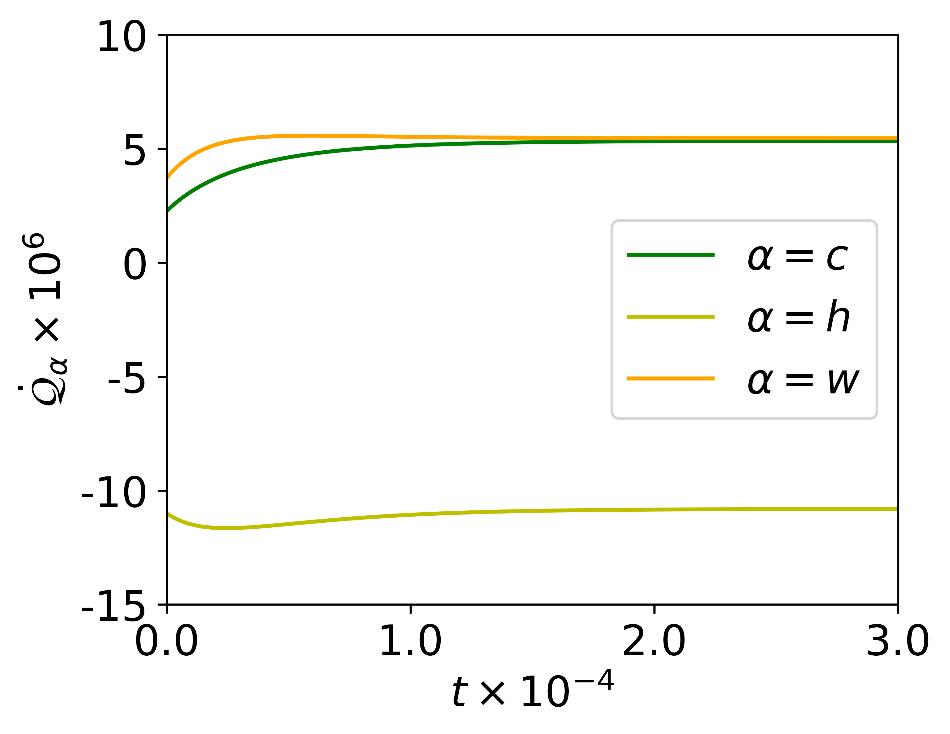
(b)

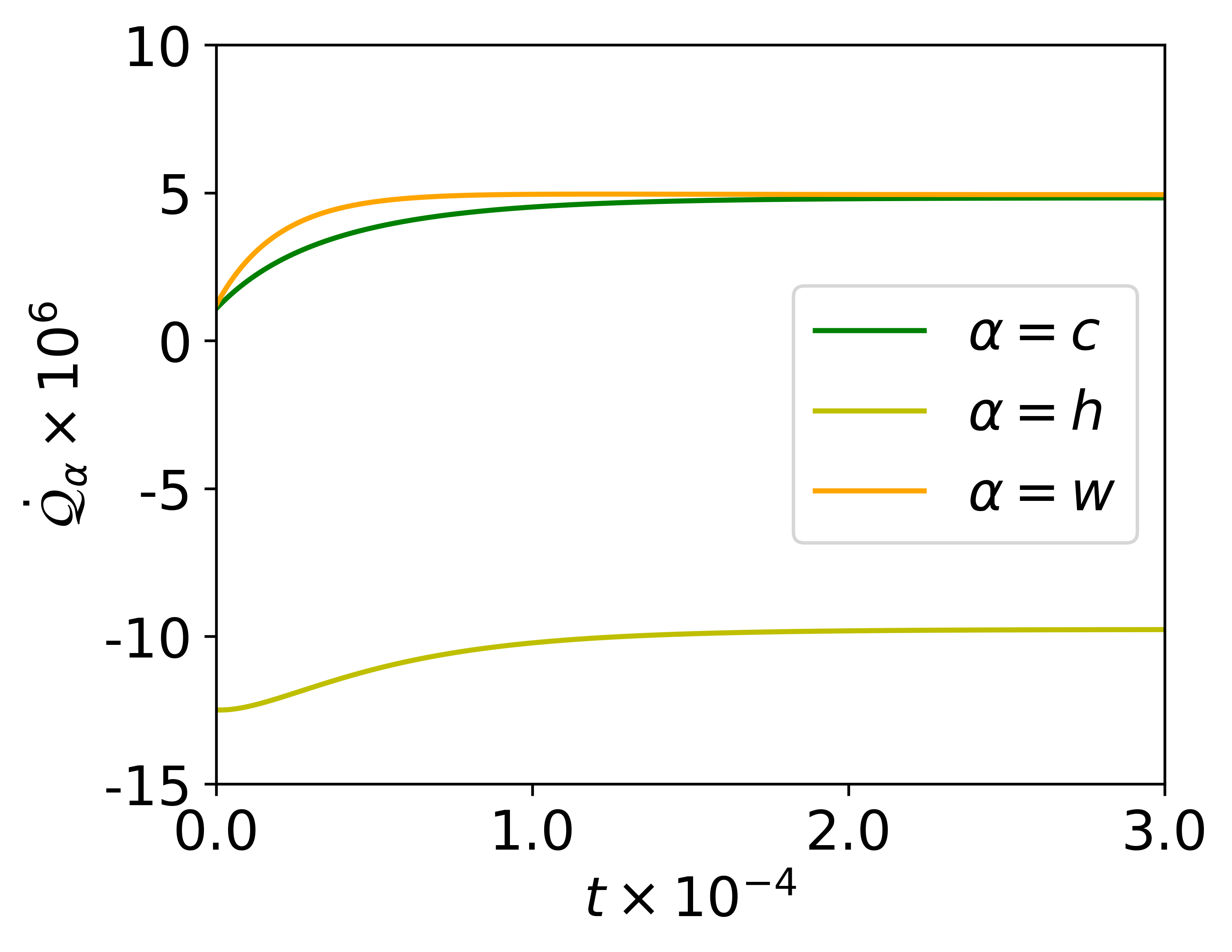
(c)

Figure 4: Time-variation of the heat currents originating from the three qubits constituting the quantum refrigerator. Time is shown along the horizontal axis and vertical axes shows the heats currents, $\dot{\mathcal{Q}}_{\alpha}$ (Eq. (22)), for the three qubits distinguished by different $\alpha$ as described in the legends of the plots. Panel (a) depicts the relevant heat currents when we choose to use harmonic-oscillator baths locally connected to the subsystems. Panels (b) and (c) describe the same, but for the case of anharmonic-oscillator baths with $\zeta=100$ and $\zeta=50$, respectively. As the values $\zeta$ decrease from left to right in this figure, the bath oscillators move further away from the harmonic regime. All the other relevant parameters are described in subsection III.2.

Now we bring our attention to the thermodynamic quantities signifying the power and efficiency of the three qubit quantum refrigerator studied in this paper. For this purpose we first compute the heat currents of all the three subsystems, which quantifies the rate of heat flow from the local heat baths to the corresponding qubits. The instantaneous heat currents are given by

$$\dot{\mathcal{Q}}_{\alpha}(t)=\text{Tr}[H_{\text{ref}}\mathcal{D_{\alpha}}(\rho_{s}(t))],$$ (22)

where the dissipator of the qubit $\alpha$ is given by $\mathcal{D_{\alpha}}(\rho_{s}(t))$, as expressed in eq. (13) and $H_{\text{ref}}$ is the Hamiltonian of the refrigerator given by eq. (4). The cooling power of the refrigerator is expressed by the heat current of the cold qubit at steady state : $\dot{\mathcal{Q}}_{c}(t\rightarrow\infty)$. A positive value of heat current indicates heat flowing out of the corresponding qubit and thereby cooling it to a temperature below that of the cold bath. For the model of absorption refrigerator described in subsection II, the coefficient of performance (COP) is measured by the ratio of the heat extracted from the cold qubit to the heat flow out of the work or engine qubit, i.e., the machine qubit, aiding the refrigeration of the cold qubit. Therefore, COP of this quantum refrigerator is given by $COP=\dot{\mathcal{Q}}_{c}/\dot{\mathcal{Q}}_{w}$. In Fig. 4 we exhibit the cooling power (marked by $\alpha=c$) along with the heat currents from the hot and work qubits as well, for heat bath composed of harmonic oscillators and anharmonic oscillators. From all the panels of Fig. 4 we can see that the heat currents from the cold and ‘work’ qubits are positive and that of the ‘hot’ qubit is negative. This implies heat flow out of the cold and ‘work’ qubit and heating of the ‘hot’ qubit and hence cooling the cold qubit as expected. However comparing Fig. 4(a) (harmonic-oscillator bath), Fig. 4(b) ($\zeta=100$) and Fig. 4(c) ($\zeta=50$), we observe that with increasing anharmonicity in the bath modes, the transient heat currents from the cold and ‘work’ qubits start with a smaller value, the ‘hot’ qubit gets dumped with higher heat current in short times with larger anharmonicty. However, in steady state all the heat currents achieve similar values irrespective of the anharmonicity of the bath oscillators, and total heat current from the whole system vanishes. This is reflected in the nature of the COP as well, demonstrated in Fig. 5. We can see that the COP of the quantum refrigerator starts of with a substantially higher value for higher anharmonicity in the bath components compared to the case if harmonic-oscillator baths were used in the three-qubit quantum refrigerator. But as time goes on, the curves exhibiting the COP of the fridges cross (marked by the red dotted line in Fig. 5), followed by a higher COP in the case of the harmonic-oscillator baths, until all the curves stabilise to the same COP in steady state. It should be noted that though the steady-state heat currents are not altered due to anharmonicity introduced in the bath oscillators, the preceding change brings down the temperature of the target qubit by a significant amount and this advantage takes over as we approach the steady state.

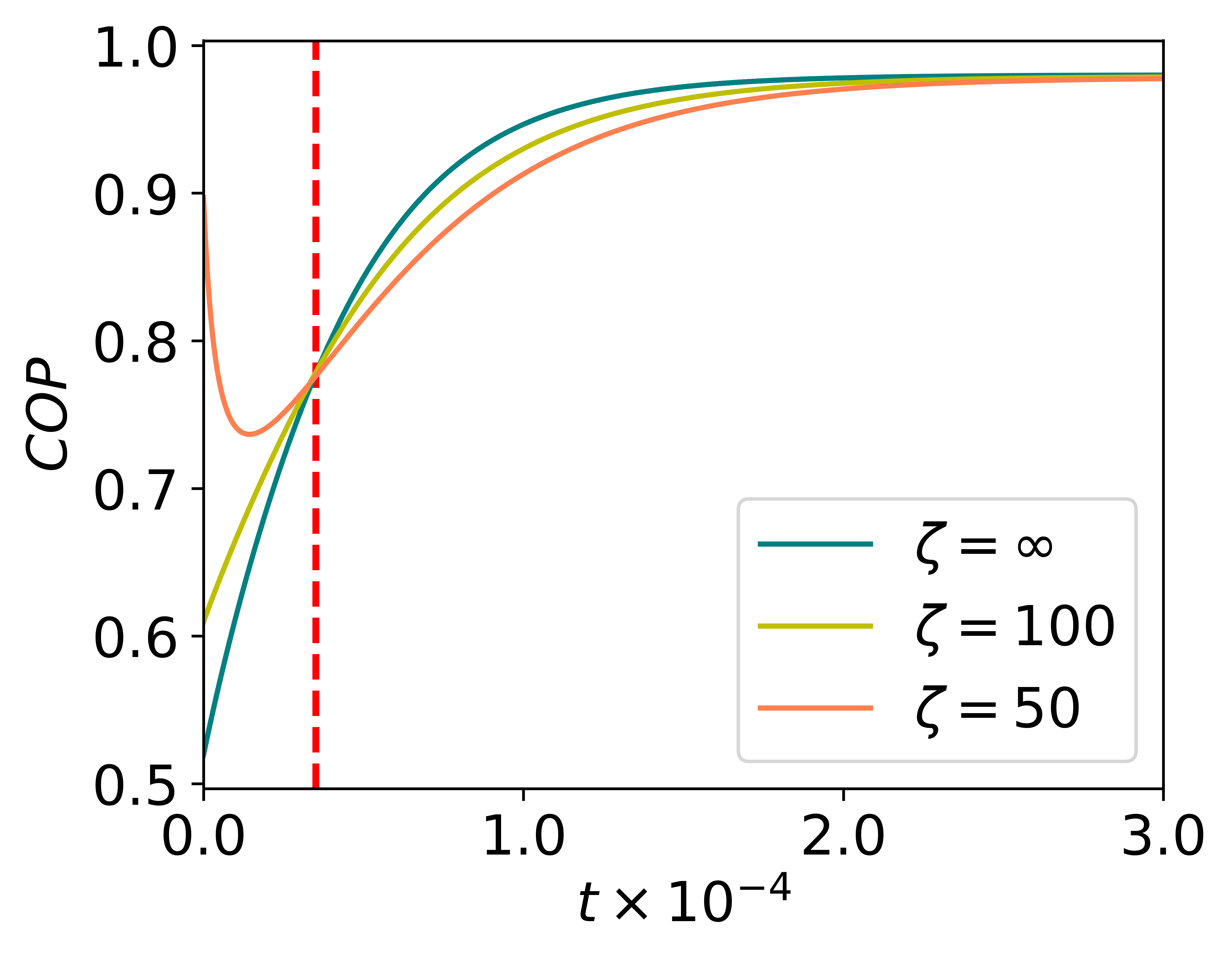
Figure 5: Time variation of the coefficient of performance (COP) of the three-qubit quantum refrigerator with different anharmonicities in the bath modes. Horizontal axis shows time and vertical axis presents COP for values of $\zeta$ described in the legend. $\zeta=\infty$ marks the harmonic limit and lower value of $\zeta$ incorporates higher anharmonicity in the bath oscillators, as described by Eq (9). The red dotted vertical line signifies the time at which the COPs for different values of $\zeta$ cross before they merge again in the steady state. The relevant system parameters are as described in subsection III.2.

IV Conclusion

In this paper, we have demonstrated the functional advantage of using Kerr-type nonlinear baths in the scheme of three-qubit quantum refrigerators, triggering significantly better steady-state cooling of the target qubit compared to the case of harmonic oscillator baths. We confine our study to the limit where system-bath coupling remains in the Markovian regime, and hence the GKSL master equation can faithfully capture the dynamics of the system. We have presented the theoretical framework to implement the effect of nonlinear thermal baths in the formalism of simulating the system evolution using quantum master equation. We have derived the decay rates in the Markovian quantum master equation due to the presence of anharmonic baths. We also show that a small amount of anharmonicity can help us acquire reasonable advantage over using harmonic baths, and we also study how this advantage scales with the mentioned anharmonicity. We also find that anharmonicities in the bath modes is not useful - in comparison to harmonic baths - in case one attempts to achieve transient cooling. It is also demonstrated that larger anharmonicity beyond a certain threshold facilitates better cooling if one considers the (time-)global minimum temperature as an indicator of the cooling capacity of the considered refrigerator, revealed by the study conducted for two sets of parameters. In general, notable advantage is achieved in steady-state cooling using anharmonic baths, and this scales with the nonlinearity in favour of better refrigeration. Such advantages in the steady-state cooling could be experimentally interesting, as catching the corresponding system in its transient regime may turn out to be technically challenging. We believe that the study makes it plausible that anharmonic baths will be found useful in studies on other quantum thermal engines like heat pumps.