Interplay of phase segregation and chemical reaction: Crossover and effect on growth laws

Abstract

By combining the nonconserved spin-flip dynamics driving ferromagnetic ordering with the conserved Kawasaki-exchange dynamics driving phase segregation, we perform Monte Carlo simulations of the nearest neighbor Ising model. Such a set up mimics a system consisting of a binary mixture of isomers which is simultaneously undergoing a segregation and an interconversion reaction among themselves . Here, we study such a system following a quench from the high-temperature homogeneous phase to a temperature below the demixing transition. We monitor the growth of domains of both the winner, the isomer which survives as the majority and the loser, the isomer that perishes. Our results show a strong interplay of the two dynamics at early times leading to a growth of the average domain size of both the winner and loser as $\sim t^{1/7}$, slower than a purely phase-segregating system. At later times, eventually the dynamics becomes reaction dominated, and the winner exhibits a $\sim t^{1/2}$ growth, expected for a system with purely nonconserved dynamics. On the other hand, the loser at first show a faster growth, albeit, slower than the winner, and then starts to decay before it almost vanishes. Further, we estimate the time $\tau_{s}$ marking the crossover from the early-time slow growth to the late-time reaction dominated faster growth. As a function of the reaction probability $p_{r}$, we observe a power-law scaling $\tau_{s}\sim p_{r}^{-x}$, where $x\approx 1.05$, irrespective of temperature. For a fixed value of $p_{r}$ too, $\tau_{s}$ appears to be independent of temperature.

I INTRODUCTION

Nonequilibrium dynamics of a system following a quench from a high-temperature disordered state to a temperature below the critical temperature $T_{c}$, marking an order-disorder phase transition, has been an active research topic over the last five decades Bray (2002); Puri and Wadhawan (2009). Typical examples of order-disorder transitions are ferromagnetic ordering and phase segregation in a binary mixture. The equilibrium aspects of these transitions, viz., values of static critical exponents, bear universal features Stanley (1971); Fisher (1974); Hohenberg and Halperin (1977); Domb et al. (1972-2001). On the other hand, the corresponding nonequilibrium kinetics of the transitions may belong to different universality classes depending on the intrinsic transport mechanism of the system Siggia (1979); Furukawa (1985, 1987). However, phenomenology of both the transitions is highlighted by the formation and growth of domains of aligned magnetic spins or like-species. Importantly, the concerned domain growth is a scaling phenomenon Bray (2002); Puri and Wadhawan (2009), i.e., various morphology-characterizing functions, viz., the two-point equal-time order parameter correlation function $C(r,t)$ and the structure factor $S(k,t)$, respectively, obey the relations

$$C(r,t)\equiv\tilde{C}(x);~{}x=r/\ell(t),$$ (1)

and

$$S(k,t)\equiv\ell(t)^{d}\tilde{S}(x);~{}x=k\ell(t),$$ (2)

where $\tilde{C}(x)$ and $\tilde{S}(x)$ are time ($t$)-independent scaling functions, $d$ is the system dimensionality, and $\ell(t)$ is the time-dependent characteristic length scale measuring the average domain size. In general, $\ell(t)$ grows in a power-law fashion as

$$\ell(t)\sim t^{\alpha}.$$ (3)

The growth exponent $\alpha$ depends on the intrinsic dynamics of the system. While for ferromagnetic ordering $\alpha=1/2$ representing the Lifshitz-Cahn-Allen (LCA) law Allen and Cahn (1979), for a solid binary-mixture phase segregation $\alpha=1/3$ stands for the Lifshitz-Slyozov (LS) law Lifshitz and Slyozov (1961); Lifshitz (1962).

In ferromagnetic ordering or phase ordering, typically one starts with a system having magnetization $m\approx 0$, and after the quench the system approaches its new equilibrium state where $m\neq 0$. The intrinsic dynamics of this phenomenon is nonconserved, as the order parameter $m$ changes continuously during the evolution. Conversely, during phase segregation in a binary mixture following a quench from a homogeneous or miscible phase, the order parameter, i.e., the concentration difference $\chi$ between the two species, remains constant throughout the evolution. Thus, its dynamics is said to be conserved. Monte Carlo simulations (MC) of the nearest neighbor Ising model has been used extensively to study domain growth in both conserved and nonconserved systems, and the corresponding growth laws have been verified Bray (2002); Marko and Barkema (1995); Amar et al. (1988); Majumder and Das (2010, 2011a, 2013a). Recently, the interest has shifted toward investigating domain growth in more complex and computationally demanding systems, e.g.,the long-range Ising model with power-law interaction, using both conserved and nonconserved order-parameter dynamics Christiansen et al. (2019, 2020, 2021); Müller et al. (2022).

In this work, by means of MC simulations of the Ising model, we investigate the effects of combining conserved and nonconserved dynamics, on the domain-growth laws. The motivation of studying such a system stems from understanding the nonequilbrium dynamics of a binary mixture where an interconversion reaction among the components occurs simultaneously with segregation among themselves. Typical example of such a system undergoing interconversion reaction is isomeric mixtures, e.g., conversion of cis-isomer to trans-isomer, or conversion between optical isomers or enantiomers McNaught et al. (1997). Either naturally or due to some external drive the components of the isomeric mixture do segregate from each other, and in combination with the interconversion reaction the mixture gets enriched with one of the isomers Soai et al. (1995); Shibata et al. (1996a, b); Tran-Cong and Harada (1996); Tran-Cong et al. (1997); Ohta et al. (1998); Viedma (2005); Lombardo et al. (2009). There have been few studies on this kind of systems either by using MC simulations of the Ising model or by solving the corresponding Cahn-Hilliard-Cook (CHC) equation Glotzer et al. (1994); Puri and Frisch (1994); Glotzer et al. (1995); Singh et al. (2012); Shumovskyi et al. (2021). While most of the studies were motivated to understand the amplification of one of the phases, the CHC approach focused on the domain-growth laws reporting a crossover from early-time reaction controlled LCA behavior to a late-time diffusion controlled LS behavior Singh et al. (2012). Interest has also been laid on considering reactions in solution via molecular dynamics (MD) simulations Longo and Anisimov (2022). Even studies with forceful preservation of the compositions being imposed along with the interconversion reaction have also been conducted, leading to fascinating pattern formation mimicking morphology of microphase separation found in the biological world Longo et al. (2023). Lately, using the Ising model it has been shown that the Arrhenius behavior of the interconversion gets significantly affected due to the simultaneous existence of the segregation process Thwal and Majumder (2023).

The effective dynamics of the system described above is nonconserved, i.e., in the final state one of the reacting species will survive as the majority which we refer to as the winner and the other one as loser. Recently, one of us has demonstrated how to disentangle the growth of the winner from the loser during phase ordering Majumder (2023). Importantly, such a disentanglement allows one to realize the scaling laws associated with domain growth using systems with relatively smaller size. Here, adopting the same disentanglement protocol we study the growth of the winner and loser in a binary mixture of isomers which is undergoing both segregation and an interconversion reaction. This not only allows us to have an appropriate realization of the associated domain-growth laws, but also to extract a timescale that marks the crossover between the two types of dynamics present in the system.

The rest of the paper is arranged in the following manner. In the next section we present details of the model we used and an elaborate description of the performed MC simulations. Following that in Sec. III we present the results and wherever required also describe the calculations of relevant observables. Finally, we conclude in Sec. IV by providing a brief summary and a future outlook.

II Model and Method

To model a binary isomeric mixture ($A_{1}+A_{2}$) undergoing interconversion reaction we use the nearest neighbor Ising model having the Hamiltonian

$$\mathscr{H}=-J\sum_{\langle ij\rangle}S_{i}S_{j},$$ (4)

where the spin $S_{i}=+1(\rm{or}~{}-1)$ represents the component $A_{1}({\rm or}~{}A_{2})$ of the mixture, and $J~{}(=1)$ is the strength of interaction. The sign $\langle\dots\rangle$ denotes that only nearest-neighbor interactions are considered. We consider our system to be a square lattice ($d=2$) having a linear dimension $L$, and apply periodic boundary condition (pbc) in all directions. The Ising model in a square lattice with pbc undergoes a phase transition with a critical temperature Onsager (1944)

$$T_{c}=\frac{2J}{k_{B}\ln(1+\sqrt{2})},$$ (5)

where $k_{B}$ is the Boltzmann constant. For a binary mixture the critical temperature is equivalent to the demixing transition temperature.

We consider that the components are undergoing the following interconversion reaction

$$A_{1}\rightleftharpoons A_{2}.$$ (6)

At the same time they are also spontaneously segregating from each other, energetics of which is captured by the Hamiltonian in Eq. (4). As already mentioned, we perform MC simulations of the above model where one needs to incorporate the dynamics of both the processes. The dynamics of the interconversion reaction in Eq. (6) is effectively mimicked by the Glauber spin-flip move, used for capturing the nonconserved dynamics of phase ordering Glauber (1963); Newman and Barkema (1999); Landau and Binder (2021). There one randomly picks up a spin on the lattice, and flips it upside down. The dynamics of segregation between the components is introduced via the Kawasaki spin-exchange move, typically used for simulating phase segregation, where the dynamics is conserved Kawasaki (1966); Newman and Barkema (1999); Landau and Binder (2021). In this move, one randomly picks up a pair of nearest-neighbor spins and exchange their positions. In our simulations we attempt both the moves and accept them using the Metropolis criterion with the probability Newman and Barkema (1999); Landau and Binder (2021)

$$p_{i}={\rm min}[1,\exp(-\Delta E/k_{B}T)],$$ (7)

where $\Delta E$ is the change in energy due to the attempted move and $T$ is the temperature. For convenience we choose $k_{B}=1$.

As the initial condition for our simulation we prepare a homogeneous $50:50$ binary mixture of $A_{1}$ and $A_{2}$ by placing them randomly on the lattice sites. This mimics a high-temperature disordered state. We then set the temperature to $T<T_{c}$ in our simulations, where we also introduce a relative weightage between the nonconserved and conserved moves using a parameter called the reaction probability $p_{r}$. It denotes the probability of attempting the Glauber spin-flip move at each MC step. Thus, the Kawasaki spin-exchange attempt is performed with a probability $1-p_{r}$. We perform simulations for a range of values of $p_{r}\in[10^{-4},10^{-1}]$. We choose the unit of time to be one MC sweep (MCS), which corresponds to $L^{2}$ attempted MC moves. The unit of temperature is chosen to be $J/k_{B}$, and all the results are for a system with $L=128$ containing $L^{2}=16384$ number of spins or isomers. All the simulations are run until $10^{7}$ MCS, which is sufficient to extract meaningful results for the chosen system size considering the covered variations of $T$ and $p_{r}$. Except for the time evolution snapshots all subsequently presented results are averaged over $20$ independent initial configurations, obtained by using different seeds in the random number generator.

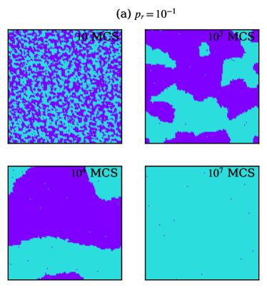
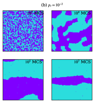
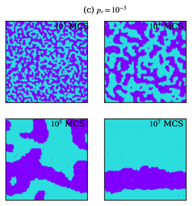
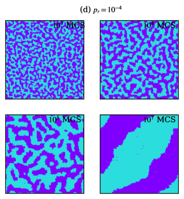
Figure 1: Snapshots at different times representing the evolution of a binary mixture of isomers ($A_{1}+A_{2}$), where an interconversion reaction is occurring simultaneously with segregation. The initial system is a homogeneous $50:50$ mixture of the two isomers in a square lattice of linear dimension $L=128$, mimicking a configuration above the critical temperature $T_{c}$, which is then quenched to a temperature $T=0.5T_{c}$. Results are presented for different values of the reaction probability $p_{r}$, as indicated. The two colors correspond to the location of the two different isomers on the lattice.

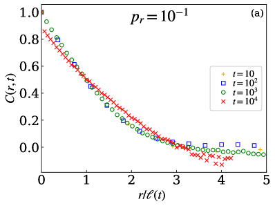
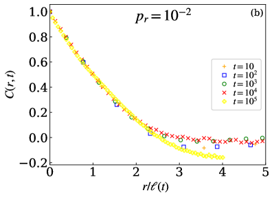
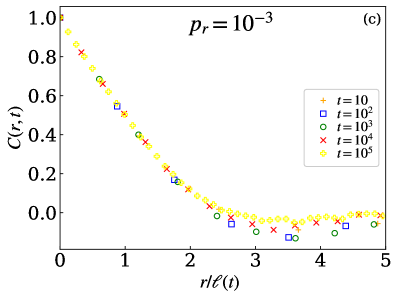
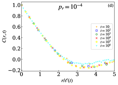
Figure 2: Plots of the two-point equal-time correlation function $C(r,t)$ as a function of the scaling variable $r/\ell(t)$ at different times for different values of the reaction probability $p_{r}$, as indicated. Here, the average domain length $\ell(t)$ is calculate from the crossing of the unscaled data of $C(r,t)$, using the condition prescribed in Eq. (9). See text for details. All results are at a temperature $T=0.5T_{c}$ for a system of size $L=128$.

III Results

In this section we present our main results. It is further divided into two subsections. In the first subsection, we deal with simulation results at a fixed temperature $T=0.5T_{c}$. In the second, we present results obtained for variation of $T$.

III.1 Dynamics at ${T=0.5T_{c}}$

Here we present results for a fixed quench temperature $T=0.5T_{c}$. The effect of slow dynamics at low $T$ and difficulty of estimating various observables at high $T$ due to thermal noise are negligible at such a moderate $T$. In Figs. 1(a)-(d) we present time evolution snapshots for different reaction probability $p_{r}$. As expected, the time evolution at the largest $p_{r}$, shown in Fig. 1(a), bears almost a perfect resemblance with time evolution during ferromagnetic ordering. There one can hardly notice any effect of phase segregation as the dynamics of the chemical reaction dominates throughout the evolution, and one eventually ends up with one of the isomers as the majority or winner, equivalent to the final magnetized state obtained during ferromagnetic ordering. As $p_{r}$ decreases, gradually the effects of phase segregation show up. For $p_{r}=10^{-3}$ and $10^{-4}$ one can clearly notice the bicontinuous domain morphology at early times, a classic signature of spinodal decomposition in a phase-segregating system Marko and Barkema (1995); Majumder and Das (2010, 2011a). Eventually, the reaction takes over at later times and the system approaches toward a state where one of the isomers emerges as the winner. For very small $p_{r}$ this dynamics slows down as one can appreciate from the snapshot shown at the latest time for $p_{r}=10^{-4}$. Since, the focus of this paper is on the domain-growth laws and its crossover dynamics, here, we do not explore the kinetics of the interconversion reaction, and rather refer to Ref. Thwal and Majumder (2023) for that.

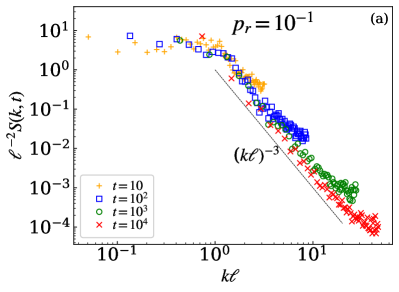
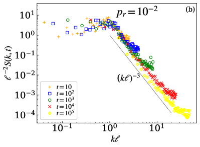
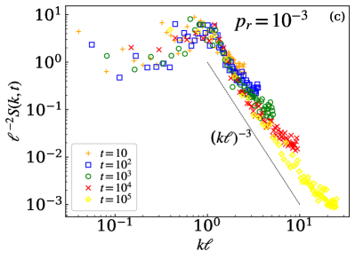
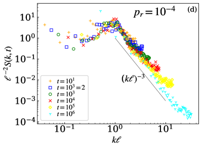
Figure 3: Scaling plots of the structure factor $S(k,t)$ at different times, for different values of the reaction probability $p_{r}$, as indicated. Here also, the average $\ell(t)$ used is obtained from $C(r,t)$. The dashed line at large $k$ represents the Porod’s tail. The results are for the same systems as presented in Figs. 2.

It is clear from the time evolution snapshots that the pattern morphologies while the system is evolving is affected by the two competing dynamics. As a first check we calculate the two-point equal-time correlation function

$$C(r,t)=\langle S_{i}Sj\rangle-\langle S_{i}\rangle\langle S_{j}\rangle,$$ (8)

where $r=|i-j|$ is the distance between the spins at lattice sites $i$ and $j$. Following the traditional approach we extract the average domain length $\ell(t)$ using the criterion

$$C[r=\ell(t),t)]=\frac{1}{2}C(0,t).$$ (9)

Using this $\ell(t)$, in Figs. 2(a)-(d) we plot $C(r,t)$ against the scaled variable $r/\ell(t)$ at different times to verify the scaling quoted in Eq. (1), for different values of the reaction probability $p_{r}$. For the largest $p_{r}$, presented in Fig. 2(a) we obtain a reasonably good collapse of data for different times until the finite size effect is experienced at $t\approx 10^{4}$. Such a behavior is expected for ferromagnetic ordering. As $p_{r}$ decreases one notices that in Fig. 2(b) the data collapse is reasonable only for intermediate times. Absence of data collapse for $t=10$ and $10^{2}$ suggests that the system is still under the effect of phase segregation. At the latest time the data again are affected by the finite size of the system. With further decrease of $p_{r}$, the data in Figs. 2(c) and (d) show reasonably good collapse until $t=10^{4}$, however, with an oscillating behavior around zero at large $r$, typical of conserved dynamics of phase segregation. Note that since the dynamics for very small $p_{r}$ is slow, the system is not expected to experience any finite-size effects until $t\approx 10^{5}$. Thus, the non-collapsing behavior of the data at $t=10^{5}$ in Figs. 2(c) and (d) can only be attributed to the dominance of the interconversion reaction.

The scaling behavior in the kinetics can be also probed by another quantity, i.e., the structure factor which is determined by the Fourier transform

$$S(\mathbf{k},t)=\int d\mathbf{r}C(\mathbf{r},t)e^{i\mathbf{kr}}.$$ (10)

In Figs. 3(a)-(d) we verify the scaling of $S(k,t)$, embedded in Eq. (2). Like the data for $C(r,t)$, for $p_{r}=10^{-1}$ the behavior of $S(k,t)$ in Fig. 3(a) is reminiscent of a typical ferromagnetic ordering. However, with decreasing $p_{r}$, the data presented in Figs. 3(b)-(d) show reasonably good collapse, i.e., the data cannot unambiguously capture the interplay of the conserved phase segregation dynamics and the nonconserved dynamics due to the interconversion reaction. Noticeable is of course the power-law behavior of the tail, independent of time and $p_{r}$. The dashed lines in Figs. 3 show the consistency of this power-law decay with the generalized Porod law for scalar order parameter given as Porod (1982)

$$S(k,t)\sim k^{-(d+1)}.$$ (11)

Here the power-law exponent is $d+1=3$, mentioned next to the dashed lines. Thus, it seems that the Porod-tail behavior is unaffected by the interplay of the two dynamics.

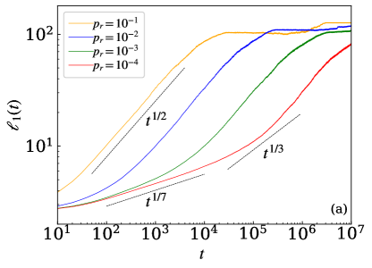
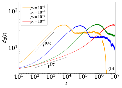
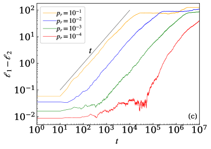
Figure 4: Double-log plots of the time dependence of the average domain size (a) of the winner $\ell_{1}(t)$ and (b) the loser $\ell_{2}(t)$, for different reaction probability $p_{r}$, obtained from simulations using a system of size $L=128$ at $T=0.5T_{c}$. In (c) we show the corresponding time dependence of the difference $\ell_{1}-\ell_{2}$, for different $p_{r}$. The dashed lines in all the figures represent different power-law behaviors as mentioned.

Next, we move on to explore the interplay of dynamics via the time dependence of the growing sizes of the domains. As shown previously by one of us that disentanglement of the kinetics of the winner from the loser allows one to realize the growth laws unambiguously, here also, we rely on the same Majumder (2023). Thus, rather than using the average domain size $\ell(t)$, at a given time we estimate the average domain size $\ell_{1}(t)$ of the winner and also $\ell_{2}(t)$ of the loser. For a detail on how these lengths are estimated, we refer to Ref. Majumder (2023). The measured domain lengths of the winner for different $p_{r}$ are presented in Fig. 4(a) on a double-log scale. The data for $p_{r}=10^{-1}$ show a single growth regime, consistent with a $\ell_{1}(t)\sim t^{1/2}$ power-law behavior, i.e., the LCA law. The flat behavior following the power-law growth indicates that finite-size effects have started showing up. At even later times, one sees a jump that correspond to an avalanche Olejarz et al. (2013); Majumder (2023). As $p_{r}$ decreases an initial regime with a much slower growth emerges, by virtue of the dominance of phase segregation dynamics over the interconversion reaction dynamics. At later times, one sees again a growth consistent with the LCA law. The duration of the initial slow regime gets extended as $p_{r}$ decreases. In fact for $p_{r}=10^{-4}$, within the given maximum simulation time, the slowest regime appears to be longer lived. The data for $p_{r}=10^{-3}$ follow the data for $p_{r}=10^{-4}$ until $t\approx 500$, when the reaction dynamics takes over. The data for $p_{r}=10^{-4}$ continues to grow slowly, consistent with a $\ell_{1}\sim t^{1/7}$ behavior, which is much slower than the expected LS behavior $\ell_{1}\sim t^{1/3}$ for a phase-segregating system. This implies that the growth of the domains slows down significantly in presence of an interconversion reaction. On the other hand, when the domains of the two isomers are well separated, phase segregation seizes and the dynamics is entirely controlled by the interconversion reaction. Hence, at late times the LCA behavior is always realized as shown by the data for all $p_{r}$.

In Fig. 4(b) we show the time dependence of the average domain size $\ell_{2}(t)$ of the loser for different $p_{r}$. There also for $p_{r}=10^{-1}$ one sees a single growth regime followed by a plateau before it suddenly vanishes due to the avalanche effect, also observed as a corresponding abrupt increase of $\ell_{1}(t)$ in Fig. 4(a). In the power-law regime, the growth is consistent with $\ell_{2}(t)\sim t^{0.45}$, albeit, slower than what is observed for the corresponding $\ell_{1}(t)$. With decreasing $p_{r}$ a slower early-time regime emerges like in the time dependence of $\ell_{1}(t)$. Here, also the early-time regime gets extended as $p_{r}$ decreases. For $p_{r}=10^{-4}$ the growth in this early-time regime is consistent with a $\ell_{2}(t)\sim t^{1/7}$ behavior, similar to what is observed for the corresponding $\ell_{1}(t)$ in Fig. 4(a). This indeed confirms that in this early-time regime the dynamics is controlled by the phase segregation, however, the occurrence of the interconversion reaction every now and then makes the dynamics slower than the LS growth, expected for an ideally phase-segregating system. For smaller $p_{r}$ the very late-time behavior is not observed within the given maximum simulation time. Overall, from the plots presented in Figs. 4(a) and (b) we infer that during the evolution initially the phase segregation is dominant with occasional involvement of the interconversion reaction, and thus the growth of the domains of the isomers in this regime is even slower than LS law. However, at later times phase segregation is no more capable of driving the system, as either the system has completely phase segregated or the domains of the individual isomers are very well separated. Hence at reaction-dominated late times, the dynamics is perfectly consistent with the LCA law, expected for ferromagnetic ordering.

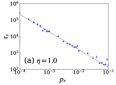
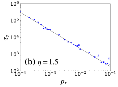
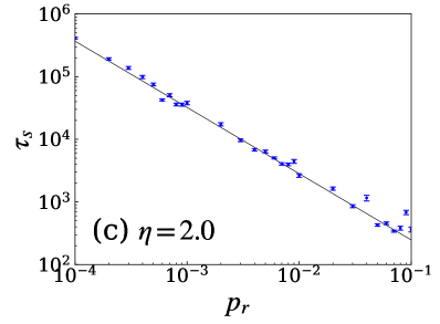
Figure 5: Double-log plots of the crossover time $\tau_{s}$ as a function of the reaction probability $p_{r}$, at $T=0.5T_{c}$ using a system of size $L=128$, for different choices of the parameter $\eta$ in Eq. (13). The dashed lines are the best fits obtained using the ansatz in Eq. (14). For details see the main text.

The other important aspect of the kinetics is of course the time scale when the system crosses over to the reaction dominated regime. This crossover is more clearly visible if one plots the time dependence of the difference between the domain length of the winner and loser, i.e., $\ell_{1}-\ell_{2}$, as presented in Fig. 4(c) for the data in Figs. 4(a) and (b). In this case the behavior is almost similar for all $p_{r}$. Initially for a certain period, $\ell_{1}-\ell_{2}$ remains constant followed by a steady growth consistent with the dashed line representing

$$\ell_{1}-\ell_{2}\sim t,$$ (12)

i.e., linear behavior with time. It can be easily noticed that the time when the flat behavior of $\ell_{1}-\ell_{2}$ switches over to a linear growth, shifts toward right with decrease in $p_{r}$. From this time onward the growth of $\ell_{1}$ is significantly faster than the corresponding growth in $\ell_{2}$, thus indicating a crossover to the reaction dominated dynamics. Based on this observation we define the crossover time $\tau_{s}$ from segregation to reaction dominated regime such that it satisfies the relation

$$\ell_{1}(\tau_{s})-\ell_{2}(\tau_{s})=\eta,$$ (13)

where $\eta$ prescribes how much difference between $\ell_{1}$ and $\ell_{2}$ is considered. In Figs. 5(a)-(c) we show the plots of $\tau_{s}$ as a function of $p_{r}$ for three different choices of the parameter $\eta$ in Eq. (13). There the errors are estimated from a Jackknife analysis, where $\tau_{s}$ is calculated independently for each Jackknife bin that contains all but data from one of the $20$ initial realizations we used Efron (1982). The apparent linear behavior of the data on a double-log scale implies a power-law dependence of $\tau_{s}$ on $p_{r}$. To quantify this power-law behavior we write down the following ansatz

$$\tau_{s}=Ap_{r}^{-x},$$ (14)

where $A$ is a prefactor and $x$ is the power-law exponent. We fit this ansatz to our data, the results of which are tabulated in Table 1. In Figs. 5(a)-(c), the dashed lines represent the obtained best fits. The results suggest that although the prefactor $A$ increases with $\eta$, the estimated exponent $x\approx 1.07$ is very weakly dependent on the choice of $\eta$. Hence, for all subsequent estimation of $\tau_{s}$ we rely only on the choice $\eta=1$.

Table 1: Fitting results for $\tau_{s}$ vs. $p_{r}$ data presented in Figs. 5, using the ansatz in Eq. (14).

$\eta$	$A$	$x$
$1.0$	$11.12\pm 1.1$	$1.08\pm 0.02$
$1.5$	$15.53\pm 1.6$	$1.08\pm 0.02$
$2.0$	$21.63\pm 2.1$	$1.06\pm 0.02$

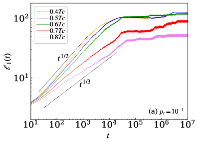
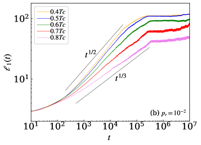
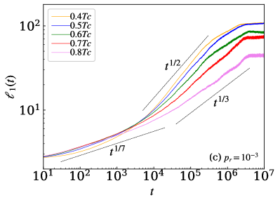
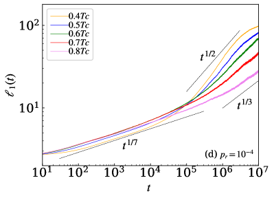
Figure 6: Double-log plots of the time dependence of the average domain size of the winner $\ell_{1}(t)$ at different temperatures for different reaction probability $p_{r}$, using a system of size $L=128$. The two dashed lines representing power laws $\ell_{1}\sim t^{1/2}$ and $\ell_{1}\sim t^{1/3}$ are respectively, the LCA and LS growths. In (c) and (d) an additional dashed line representing the power-law $\ell_{1}\sim t^{1/7}$ is also shown for the initial regime.

III.2 Temperature dependence of the dynamics

In this subsection we investigate the temperature dependence of the kinetics. For that purpose we perform simulations for different values of the reaction probability $p_{r}$, at different temperatures below $T_{c}$.

Here, we do not present the time evolution snapshots for different temperatures, and rather straight away move on to the time dependence of the average domain sizes. We start with plots of the average domain size $\ell_{1}(t)$ of the winner in Figs. 6, for five different temperatures. For the largest reaction probability, i.e., $p_{r}=10^{-1}$, presented in Fig. 6(a), the growth of $\ell_{1}(t)$ consists of a single regime for all $T$. At moderate temperatures, i.e., $T=0.4T_{c}$, $0.5T_{c}$ and $0.6T_{c}$, this growth seem to be consistent with the LCA law $\ell_{1}\sim t^{1/2}$. However, for higher $T$, significant deviation from the LCA law is observed as the growth becomes slower with increase in $T$. The inconsistency of the data with the other dashed line implies that the slow growth is certainly faster than the LS growth $\ell_{1}(t)\sim t^{1/3}$. Also, at high $T$ there is no chance of dynamic freezing Spirin et al. (2001). Thus, the apparent slow growth can be attributed to the presence of significantly large noise clusters at high $T$ that does not allow estimation of $\ell_{1}(t)$ from a pure domain morphology of the winner. This reasoning can further be appreciated from the fact that at very late time when the reaction has almost finished, $\ell_{1}(t)$ is supposed to be saturated at a value $\approx L$, at high $T$ this happens at $\ell_{1}(t)<L$. This problem can of course be tackled by appropriate noise removal technique Majumder and Das (2010, 2011a, 2013a). Nevertheless, we abstain ourselves from doing so and rather stress that the observation of a single growth regime independent of $T$ suggests a reaction dominated dynamics for $p_{r}=10^{-1}$ at all $T$.

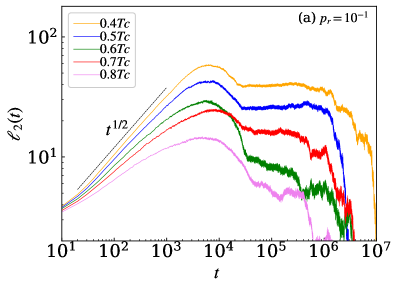
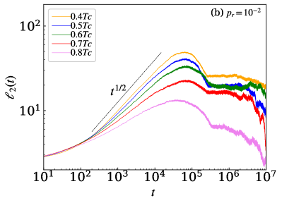
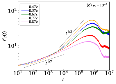
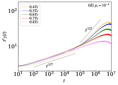
Figure 7: Double-log plots of the time dependence of the average domain size of the loser $\ell_{2}(t)$ at different temperatures for different reaction probabilty $p_{r}$, using a system of size $L=128$. The dashed line representing power law $\ell_{2}\sim t^{1/2}$ is for the LCA growth. In (c) and (d) $\ell_{2}(t)\sim t^{1/7}$ for the initial regime is also shown as a dashed line.

As $p_{r}$ decreases one can clearly see the emergence of an initial slow-growth regime for $\ell_{1}(t)$ at all temperatures. As shown in Fig. 6(b), for $p_{r}=10^{-2}$ the initial slow-growth regime is very short lived as there still the reactions start to control the dynamics from early time. Followed by the slow growth, $\ell_{1}(t)$ shows a faster growth that is again consistent with the LCA law at moderate temperatures. Again, for higher temperatures the growth although faster than the LS growth, is apparently significantly slower than the LCA law which again could be atrributed to the effect of noisy clusters while estimating $\ell_{1}(t)$.

For even smaller $p_{r}$, presented in Figs. 6(c) and (d), the initial slow regime of $\ell_{1}(t)$ is long lived and prominent. Consistency of the data at all $T$ with the power-law behavior $\ell_{1}\sim t^{1/7}$ suggests its robustness. At later times the data crosses over to a faster growth when the dynamics is dominated by the interconversion reaction. The growth then again is consistent with the LCA law for moderate $T$. At high $T$, for both $p_{r}=10^{-3}$ and $10^{-4}$ the data again show significant deviation from the LCA law. For $p_{r}=10^{-4}$ at $T=0.8T_{c}$ the data even seem to be consistent with a $\ell_{1}(t)\sim t^{1/3}$ behavior. However, we stress that this is just a mere coincidence and should not be treated as the realization of the LS behavior. In fact, this slow growth at late time as already mentioned is an artifact of the estimation of $\ell_{1}(t)$ from impure domain morphology at high $T$.

The temperature dependence of the average domain size of the loser $\ell_{2}(t)$ corresponding to the cases discussed above are presented in Figs. 7. For the largest value of $p_{r}=10^{-1}$, shown in Fig. 7(a), the comparative behavior among different $T$ is similar to what is observed for $\ell_{1}(t)$ in Fig. 6(a). At the lowest $T$ the data is consistent with the LCA law. At later times the data show a flat behavior before eventually they decay and almost vanish. As $T$ increases the behavior is similar, except for the fact that the growth becomes slower, which again is due to the fact that the estimated $\ell_{2}(t)$ is not from a pure domain morphology. Noticeable is that the time taken by $\ell_{2}(t)$ to almost vanish, decreases as $T$ increases. This is a signature of the fact that for $p_{r}=10^{-1}$, the total reaction time or kinetics of the reaction follows an Arrhenius behavior Thwal and Majumder (2023).

The behavior of the data for $p_{r}=10^{-2}$, presented in Fig. 7(b) is similar to what is observed for $p_{r}=10^{-1}$. At low $T$, in the growth regime again the data are almost consistent with the LCA law, and deviate significantly as $T$ increases. Following a brief period of flat behavior, $\ell_{2}(t)$ start to decay and almost vanishes at late times. The trend of the data again indicates an Arrhenius behavior. With further decrease of $p_{r}$, within the growth regime there exists two sub regimes as shown by the plots presented in Figs. 7(c) and (d), like what is observed for $\ell_{1}(t)$ in Figs. 6(c) and (d). The initial slow-growth regime here is consistent with the power law $\ell_{2}(t)\sim t^{1/7}$, similar to how $\ell_{1}(t)$ behaves. This confirms that irrespective of $T$, when the reaction probability $p_{r}$ is small, initially the dynamics is almost conserved due to the dominant effect of segregation, however, it is much slower than the LS growth. At later times when the interconversion reaction starts to dominate the growth becomes faster for a brief period, albeit slower than the LCA growth, before eventually starting to decay. Within the maximum simulation time of $10^{7}$ MCS, for $p_{r}=10^{-3}$ and $10^{-4}$ the data for $\ell_{2}(t)$ do not reach the point where they almost vanish. Hence, from this data it is not possible to infer anything about the Arrhenius behavior of the interconversion reaction. In this regard we refer to Ref. Thwal and Majumder (2023) where it has been shown that for lower $p_{r}$ values, the Arrhenius behavior of the interconversion reaction gets disrupted.

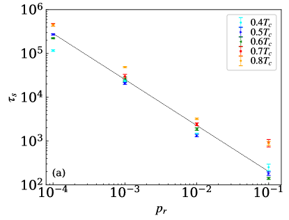
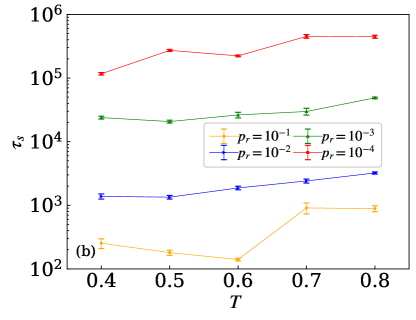
Figure 8: (a) Double-log plots of the crossover time $\tau_{s}$ as a function of the reaction probability $p_{r}$, at different $T$ using a system of size $L=128$. The dashed lines represents Eq. (14) with $A=17.97$ and $x=1.05$. (b) Variation of $\tau_{s}$ as a function of $T$, for fixed $p_{r}$ as mentioned.

Table 2: Fitting results for $\tau_{s}$ vs. $p_{r}$ data at different temperatures using the ansatz in Eq. (14).

$T$	$A$	$x$
$0.4T_{c}$	$26.54\pm 18.8$	$0.92\pm 0.08$
$0.6T_{c}$	$12.74\pm 1.7$	$1.06\pm 0.02$
$0.7T_{c}$	$13.64\pm 6.4$	$1.13\pm 0.06$
$0.8T_{c}$	$25.81\pm 12.8$	$1.07\pm 0.07$

Now we move on to investigate the effect of temperature on the crossover time $\tau_{s}$ that marks the switch over to a completely reaction dominant dynamics. As already mentioned, $\tau_{s}$ is calculated using the prescription embedded in Eq. (13) with $\eta=1$. In Fig. 8(a) we show the plots of the $\tau_{s}$ as a function of $p_{r}$, at different $T$. All the data seem to be parallel to each other except for the data points at $p_{r}=10^{-1}$ for $T=0.7T_{c}$ and $0.8T_{c}$. Possibly, the crossover is not so sharp at high $T$, as rate of both phase segregation and interconversion reaction get enhanced due to huge thermal fluctuations. Hence, the criterion used in Eq. (13) fails to unambiguously extract the crossover time $\tau_{s}$. Nonetheless, we obtain reasonable results when we fit the ansatz in Eq. (14) to the data at different $T$, the results of which are tabulated in Table 2. From the values quoted there we calculate the average prefactor $A=17.97\pm 3.1$ and $x=1.05\pm 0.07$, which of course, have significant error bars. Nevertheless, in Fig. 8(a) we plot a dashed line representing Eq. (14) with the above quoted values. The data indeed look more or less parallel to the dashed line except for the points representing $p_{r}=10^{-4}$ at $T=0.7T_{c}$ and $0.8T_{c}$.

The variation of $\tau_{s}$ with $T$ for fixed values of the reaction probability $p_{r}$ are shown in Fig. 8(b). The almost flat behavior of the data for all cases indicates that the crossover is very weakly dependent on the temperature, although for purely segregating system it has been shown that the relaxation time shows an Arrhenius behavior Thwal and Majumder (2023). This of course is the courtesy of the effect of presence of interconversion reaction even when the dynamics is dominated by segregation.

IV Conclusion

To summarize, we have presented results on the effects of interplay of phase segregation and interconversion reaction on the kinetics of domain growth. For that purpose we have performed Metropolis MC simulations of the nearest neighbor Ising model in a square lattice, governed by both conserved and nonconserved dynamics. The system mimics a phase-segregating isomeric binary mixture. Starting from such a homogeneous binary mixture, we have studied the nonequilibrium kinetics when the system is quenched below the demixing or critical temperature. Due to the presence of the reaction, in the asymptotic limit one of the isomers will emerge as the winner, i.e., it will be present as the majority, and the other isomer will perish which we refer to as the loser. Instead of monitoring the average domain size of both isomers, we have studied the kinetics of both of them separately.

Our results show that for higher reaction probability $p_{r}$, the dynamics of the system resembles ferromagnetic ordering throughout the evolution. There one observes the usual scaling of the two-point equal-time correlation function $C(r,t)$ and the structure factor $S(k,t)$. As $p_{r}$ decreases, these quantities show signature of the strong interplay between the segregation dynamics and the reaction dynamics, thereby, the overall scaling picture does not hold anymore. For very low $p_{r}$, instead one observes an early-time scaling that resembles the conserved dynamics due to phase segregation. However, the universal Porod-tail behavior of $S(k,t)\sim k^{-3}$ remains unaffected for any choice of $p_{r}$.

While for large $p_{r}$ the time dependence of the average domain size of the winner $\ell_{1}(t)$ and loser $\ell_{2}(t)$ show behavior consistent with ferromagnetic ordering, with decrease of $p_{r}$ the interplay of the conserved and noconserved dynamics show up. In fact, one observes a crossover in the growth from an initial slow $\ell_{1}(t)\sim t^{1/7}$ behavior to the usual $\ell_{1}(t)\sim t^{1/2}$ growth at late times. The time dependence of $\ell_{2}(t)$ for small $p_{r}$ also show a similar crossover with initially growing similarly with the power law $\ell_{2}(t)\sim t^{1/7}$. Afterwards, of course, $\ell_{2}(t)$ grows slower than $\ell_{2}(t)\sim t^{1/2}$. At very late time $\ell_{2}(t)$ starts to decay and asymptotically almost vanishes. We caution the reader that a proper theoretical understanding of the numerically observed early-time slow growth $\sim t^{1/7}$ is still required.

The observation of the crossover in the growth prompted us to also calculate a crossover time $\tau_{s}$ from the time dependence of the difference between average domain size of the winner and loser, which at late times grows as $\ell_{1}-\ell_{2}\sim t$. Our data for $\tau_{s}$ as a function of $p_{r}$ appears to follow the power-law scaling $\tau_{s}\sim p_{r}^{-x}$, where we obtained $x=1.05$, almost independent of temperature. The crossover time $\tau_{s}$ also appears to be independent of temperature for fixed values of $p_{r}$.

A facile adaptation of this work would be to consider a more complex reaction involving more than two species, for which MC simulation of an analogous $q$-state Potts model seems to be an automatic choice Wu (1982); Majumder et al. (2018); Janke et al. (2021). In future, it would also be interesting to study the effect of such interplay of phase segregation and interconversion reaction on the other aspect of nonequilibrium dynamics of phase transition, i.e., aging and related scaling Henkel and Pleimling (2010); Midya et al. (2014, 2015). Given the recent growing interest in nonequilibrium dynamics of long-range systems, it would certainly be worth to investigate this interplay of conserved and nonconserved dynamics using the long range Ising model with power-law interaction Christiansen et al. (2019, 2020, 2021); Müller et al. (2022). Lastly, to invoke more real effects of modeling such a system it would be challenging to construct a similar model where the reaction is happening in solutions. For that one needs to perform MD simulations of a fluid-like system where the role of hydrodynamics has to be taken into account Majumder and Das (2011b, 2013b).