Revisiting quantum black holes from effective loop quantum gravity

Abstract

We systematically study a family of loop quantizations for the classical Kruskal spacetimes using the effective description motivated from loop quantum gravity for four generic parameters, $c_{o},m,\delta_{b}$ and $\delta_{c}$, where the latter two denote the polymerization parameters which capture the underlying quantum geometry. We focus on the family where polymerization parameters are constant on dynamical trajectories, and of which the Ashtekar-Olmedo-Singh (AOS) and Corichi-Singh (CS) models appear as special cases. We study general features of singularity resolution in all these models due to quantum gravity effects and analytically extend the solutions across the white hole (WH) and black hole (BH) horizons to the exterior. We find that the leading term in the asymptotic expansion of the Kretschmann scalar is $r^{-4}$. However, for AOS and CS models black holes with masses greater than solar mass the dominant term behaves as $r^{-6}$ for the size of the observable universe and our analysis can be used to phenomenologically constrain the choice of parameters for other models. In addition, one can uniquely fix the parameter $c_{o}$ by requiring that the Hawking temperature at the BH horizon to the leading order be consistent with its classical value for a macroscopic BH. Assuming that the BH and WH masses are of the same order, we are able to identify a family of choices of $\delta_{b}$ and $\delta_{c}$ which share all the desired properties of the AOS model.

I Introduction

Black holes (BHs) initially were only discovered as solutions to Einstein’s General Relativity (GR) [1] but now observations have confirmed their existence [2, 3]. However to understand these objects in entirety, GR is insufficient as it predicts its own demise near the singularities present inside BHs [4]. Spacetimes near these singularities enter the Planckian regime and it is widely believed that a quantum theory of gravity is necessary to understand these esoteric objects.

Loop quantum gravity (LQG) is a non-perturbative theory of quantum gravity [5]. Its techniques have been used to resolve the cosmological singularities, which is now a well-established research field, usually referred to as loop quantum cosmology (LQC) [6, 7, 8]. Since the interior of a static BH is isometric to the vacuum Kantowski-Sachs (KS) cosmological spacetime, techniques from LQC have been borrowed to study loop quantum black holes (LQBHs) [9]. A majority of LQBH models describe the spacetimes in an effective or semi-classical fashion, as such a description has been proved very successful in LQC [10, 11, 12], and captures the leading-order quantum corrections with the introduction of polymerization parameters. In particular, it shows explicitly that the big bang singularity is replaced by a quantum bounce (see for eg. [13, 14, 15]) and the subsequent cosmological perturbations are consistent with current observations (see for eg. [16, 8]). It is the general belief in the community that such an effective description should be also applicable to LQBHs, although a detailed derivation of the effective description from the full quantum dynamics of LQBHs is still absent. In this manuscript our analysis will assume the validity of this effective spacetime description.

In the quantum theory of LQBHs, the elementary variables are holonomies of connection variables which contribute to trigonometric functions of the connection at the level of the Hamiltonian. Different quantizations of LQBH models differ in their choices of the two polymerization parameters, $\delta_{b}$ and $\delta_{c}$, which capture the edge length of loop in the quantization procedure. At an effective level this amounts to the following replacements of the two symmetry reduced Ashtekar-Barbero connection variables $b$ and $c$ [17, 9]

$$b\rightarrow\frac{\sin(\delta_{b}b)}{\delta_{b}},\quad c\rightarrow\frac{\sin(\delta_{c}c)}{\delta_{c}},$$ (1.1)

in the classical Hamiltonian. It is clear that when $\delta_{i}\rightarrow 0\;(i=b,c)$, the classical Hamiltonian is recovered and quantum effects are expected to be negligibly small. On the other hand, such effects will become large when they are large. Generally speaking, $\delta_{b}$ and $\delta_{c}$ are functions of the phase space variables $b$, $c$ and their corresponding canonical conjugates $p_{b}$ and $p_{c}$, which are connected with the spacetime metric through Eq.(2.1). Different choices of $\delta_{b}$ and $\delta_{c}$ are frequently referred to as different schemes, and various ones are available in the literature. Among them, three major schemes can be identified:

• $\mu_{o}$-(like) schemes: Inspired by the $\mu_{o}$ scheme in LQC [18, 19], in this scheme the polymerization parameters $\delta_{b}$ and $\delta_{c}$ are fixed as constants, see, for example, [20, 21, 22, 23, 24, 25, 26, 27, 28, 29], and references therein. In these studies, the dependence of $\delta_{i}$ on some physical parameters involved in the models was considered. However, in all of them, either some inconsistencies or unexpected properties were identified. In particular, it was found that in some models physical quantities depend on the choice of the fiducial cell size, while in others singularity resolutions cannot be consistently identified with a curvature scale. For details, we refer the reader to [30]. Note that of the above choices, Corichi-Singh (CS) model overcome various problems [24], but results in a highly asymmetric mass of the white hole (WH) formed after the bounce. Later different types of models which result in symmetric value of masses of BH and WH have been developed [31, 30].

• $\bar{\mu}$-(like) schemes: Inspired by the $\bar{\mu}$ scheme in LQC [14] here the polymerization parameters are chosen to be functions of the phase space variables. This was first implemented for LQBHs in [32] and adapted later in [33]. Although this scheme has alleviated all the shortcomings of the $\mu_{o}$-scheme in cosmology [6], it fails when applied to LQBHs [30]. In particular, large quantum corrections appear near BH horizons, in which the gravitational fields are already very weak classically. Basically, this quantization does not distinguish between the coordinate and the physical singularity which is illustrated in Kasner spacetimes too [34]. Furthermore, recent work has shown that these effects are, in fact, so strong that BH/WH horizons do not exist at all [35, 36]. Instead, only transition surfaces exist, and the number of such surfaces are infinite. As a result, the corresponding spacetime is geodesically complete. This result turns out to be consistent with earlier studies on $\bar{\mu}$ quantization of Kantowski-Sachs cosmological models with matter where coordinate singularity does not exist, central singularity is eliminated and the effective loop quantum spacetime is geodesically complete [37].

  It should be noted that such large quantum effects are closely related to the use of the Kantowski-Sachs metric as describing the internal spacetimes of BHs. In particular, in the Kantowski-Sachs spacetime the physical length perpendicular to the two-spheres of the classical Schwarzschild BH vanishes not only at the BH singularity but also at its event horizon. Then, the polymerization will lead to significant quantum effects at both locations. To cure the singularity, such large effects are essential. However, these large effects at BH horizons shall lead to inconsistency physically, especially when massive BHs are considered. This is because near such massive BH horizons, the gravitational fields are classically very weak, and quantum gravitational effects are expected to be negligible.

• Dirac observables: In this scheme the polymerization parameters are particular functions of the phase space variables such that they are constant along the trajectories of the dynamical equations. To counter the problems faced by the $\mu_{o}$ and $\bar{\mu}$ schemes, Dirac-observable scheme in the extended phase space was first introduced in [38, 30, 39]. In these works the two polymerization parameters were uniquely fixed at the transition surface. For massive BHs, they are given by [30]

  $$\delta^{\text{(AOS)}}_{b} = \left(\frac{\sqrt{\Delta}}{\sqrt{2\pi}\gamma^{2}m}\right)^{1/3},$$

  $$\delta^{\text{(AOS)}}_{c} = \frac{1}{2L_{o}}\left(\frac{\gamma\Delta^{2}}{4\pi^{2}m}\right)^{1/3},$$ (1.2)

  where $\gamma$ and $m$ denote, respectively, the Barbero-Immirzi and mass parameters, $\Delta\left(\equiv 4\sqrt{3}\pi\gamma\ell_{p}^{2}\right)$ denotes the minimal area gap and $L_{o}$ the size of the fiducial cell, while $\ell_{p}$ is the Planck length. With the above choice of polymerization parameters, it was found that the corresponding LQBH has the following desirable properties: 1) The physical quantities and properties are independent of $L_{o}$. 2) The spacetime near the transition surface is symmetric. 3) There exists a universal mass-independent upper bound on the curvature invariants of the effective spacetime at the transition surface. 4) No mass amplification of the WH exists. 5) There exist negligible quantum corrections at classical scales, including the locations of massive BH/WH horizons.

In addition, working within the four-dimensional phase space, spanned by the four Ashtekar phase variables ($b,p_{b};c,p_{c}$), Dirac observables at the Hamiltonian level were also considered in [40, 41, 42, 43, 44, 45].

It is interesting to note that the Ashtekar-Olmedo-Singh (AOS) scheme can be considered as a mixture of the $\mu_{o}$ and $\bar{\mu}$ like schemes. Then, a natural question arises: Are there other choices of polymerization parameters $\delta_{b}$ and $\delta_{c}$ for which similar desirable properties as those of the AOS solution exist? The goal of this manuscript will be to explore this avenue in detail. But before we go further, it is important to note the following remark.

Remark: It is to be emphasized that the above comparison between different schemes is restricted to Kruskal spacetimes in GR. Whether the noted advantages and disadvantages extend to other black hole spacetimes and gravitational collapse scenarios is far from clear. In particular, a recent study showed that a $\mu_{o}$ like scheme would not permit formation of trapped surfaces in gravitational collapse which $\bar{\mu}$ like scheme permits generically [46]. In addition, the $\bar{\mu}$-scheme was also used in the quantization of the Lemaitre-Tolman-Bondi metric in [47, 48, 49]. Yet, another different approach was explored in [50, 51], and the model was further studied in [52].

To generalize the AOS model, following the line of previous studies of LQBHs [53, 28], we first make a general survey over the most general solutions of the effective Hamiltonian which contains five free parameters, including $\delta_{b}$ and $\delta_{c}$ which are treated as constant on dynamical trajectories. Then, using the gauge freedom, we find that one of the five free parameters can be gauged away simply by the shift of the timelike coordinate, $T\rightarrow T+T_{0}$. Hence, only four of the five free parameters are physically essential, denoted, respectively, by $c_{o}$, $m$, $\delta_{b}$ and $\delta_{c}$. It should be noted that the physical meaning of $c_{o}$ was studied in detail in [29]. However, unlike [29], in our current analysis we do not adopt the AOS choice of $\delta_{b}$ and $\delta_{c}$ given by Eq.(• ‣ I), and instead consider them as arbitrary constants. Among these four parameters, $m$ is related to the mass parameter of the solution, and $c_{o}$ characterizes not only the position of the transition surface [29], but also the Hawking temperature at the BH horizon. It should be noted that the four-parameter solutions are valid only inside the BH and WH horizons, $T_{\text{WH}}\leq T\leq T_{\text{BH}}$, where $T_{\text{WH}}$ and $T_{\text{BH}}$ denote the locations of the WH and BH horizon, respectively. To study the asymptotical behavior of the LQBH spacetime, we first extend the solutions analytically beyond these surfaces [cf. Section II.C]. Since the extension is analytical, it is also unique.

After analytically extending the solutions across the WH and BH horizons, we find the leading term in the asymptotic expansion of the Kretschmann scalar is $r^{-4}$. This result is well known for the AOS model and we find it to hold for a family of models we study. In addition to $r^{-4}$ term there also exists an $r^{-5}$ correction along with the $r^{-6}$ term that captures the classical behavior. We find that the $r^{-4}$ term becomes dominant over the $r^{-6}$ term only when $r>r_{c}$, where $r_{c}$ is the critical radius. In addition, we also calculate the value $r_{c_{4}}$, the critical radius beyond which the $r^{-4}$ term starts to dominate over the $r^{-5}$ term. Similarly, we calculate $r_{c_{5}}$ to find the dominant term among $r^{-5}$ and $r^{-6}$ term. For both the AOS and CS models, we find that $r_{c},r_{c_{4}},r_{c_{5}}>L_{\text{obs}}$ for solar mass BHs, where $L_{\text{obs}}$ denotes the size of our observational Universe. This suggests that the asymptotic behavior can still be well described by its classical limit within our observable universe. In particular, the Kretschmann scalar can be still considered as falling off like $r^{-6}$ in our observable universe.

On the other hand, requiring that the deviation of the Hawking temperature at the horizon of a massive BH from its classical counterpart be negligible, we find that $c_{o}$ is uniquely fixed [cf. Eqs. (3.22) and (3.23)] to

$$c_{o}=\frac{L_{o}\delta_{c}\gamma}{8m},$$ (1.3)

which is precisely the choice made in [24, 38, 30, 39]. Once $c_{o}$ is fixed, we find that the ratio of the BH and WH masses and the dependence of the curvatures on $m$ at the transition surface are crucially dependent on the choice of the two polymerization parameters $\delta_{b}$ and $\delta_{c}$. In particular, we find that as long as they are all inversely proportional to $m^{1/3}$, that is

$$\delta_{b}=\alpha_{b}\left(\frac{\ell_{p}}{m}\right)^{1/3},\;\;\;L_{o}\delta_{c}=\alpha_{c}\left(\frac{\ell_{p}}{m}\right)^{1/3},$$ (1.4)

where $\alpha_{b}$ and $\alpha_{c}$ are two $m$-independent otherwise arbitrary dimensionless constants, the Kretschmann scalar is always independent of $m$ [cf. Fig. 1], no matter what the values of $\alpha_{b}$ and $\alpha_{c}$ are, although the amplitude of the Kretschmann scalar indeed depends on specific values of $\alpha_{b}$ and $\alpha_{c}$. On the other hand, when any of the dependence of these two parameters on $m$ is different from $m^{-1/3}$, the amplitude of the Kretschmann scalar at the transition surface will sensitively depend on the values of $m$, as shown explicitly in Figs. 2 - 4. In addition, simply requiring the ratio of the BH and WH masses be one imposes a relation between $\alpha_{b}$ and $\alpha_{c}$ [cf. Eq.(3.34)]. In particular, assuming that $\delta_{b}$ takes the form (1.4), we find that $M_{\text{BH}}=M_{\text{WH}}$ leads to

$$\alpha_{c}=\left(\frac{\gamma^{3}\ell_{p}}{2}\right)\alpha_{b}^{4},\;\left(M_{\text{BH}}=M_{\text{WH}}\right).$$ (1.5)

Therefore, we identify a class of parameters, described by Eqs.(1.3) - (1.5) with $\alpha_{b}$ being the free parameter, which share the same properties as the AOS solution. The latter corresponds to the particular choice

$$\alpha_{b}^{\text{AOS}}=\left(\frac{\sqrt{\Delta}}{\sqrt{2\pi}\gamma^{2}\ell_{p}}\right)^{1/3}.$$ (1.6)

The rest of the paper is organized as follows: In Sec.II, starting with the KS spacetime and its classical Hamiltonian, we first obtain the effective Hamiltonian by using the replacements (1.1), and re-derive the five-parameter solutions, where $B_{o},\;p_{c}^{o},\;c_{o}$ together with $\delta_{b}$ and $\delta_{c}$ appearing in Eqs.(II.1) and (2.15) are the five parameters. But, as shown there, $B_{o}$ can be eliminated by the simple replacement, $T\rightarrow T+\hat{T}_{o}$, so only four of them are physical ones, where $p_{c}^{o}$ is related to the mass parameter $m$ via the relation $p_{c}^{o}=4m^{2}$. In the same section, we consider the marginally trapped surfaces, and found that they can happen at $\dot{p}_{c}=0$ as well as at $N\rightarrow\infty$. The former corresponds to the transition surface, and the metric crosses it smoothly, while the latter represents BH and WH horizons, as shown explicitly in Sec.II.2 and II.3. In Sec.II.3, the metric is also analytically extended beyond these two horizons. In Sec.III.1, spacetimes outside the horizons are studied, including the asymptotic and near horizon regions, while in Sec.III.2, spacetimes across the transition surface and near the WH horizon are investigated. The paper concludes in Sec.IV, where we present our main findings.

II loop quantum black holes with constant polymerization parameters

The spacetime inside a classical spherically symmetric black hole can always be written in the KS form [18]

$$ds^{2}=-N^{2}dT^{2}+\frac{p_{b}^{2}}{L_{o}^{2}\left|p_{c}\right|}dx^{2}+\left|p_{c}\right|d\Omega^{2},$$ (2.1)

where $N,\;p_{b},\;p_{c}$ are all functions of $T$ only, and $d\Omega^{2}\equiv d\theta^{2}+\sin^{2}\theta d\phi^{2}$ with $-\infty<T,\;x<\infty$, $\theta\in[0,\pi]$ and $\phi\in[0,2\pi]$. However, due to the independence of the metric on $x$, the corresponding Hamiltonian is not well defined, as it is involved in integration over $x$. Then, one usually first introduce a fiducial cell with length $L_{o}$, so that $x\in[0,L_{o}]$. Physics should not depend on the choice of $L_{o}$, so at the end of the day we can always take the limit $L_{o}\rightarrow\infty$, without loss of the generality. The functions $p_{b}$ and $p_{c}$ are the dynamical variables, which satisfy the Poisson brackets

$$\{c,p_{c}\}=2G\gamma,\quad\{b,p_{b}\}=G\gamma,$$ (2.2)

where $G$ is the Newton gravitational constant, and $b$ and $c$ are the corresponding phase space conjugate momenta of $p_{b}$ and $p_{c}$, respectively.

It should be noted that the KS metric (2.1) is invariant under the gauge transformations

$$T=f(\hat{T}),\quad x=\alpha\hat{x}+x_{o},$$ (2.3)

via the redefinition of the lapse function and the length of the fiducial cell,

$$\hat{N}=Nf_{,\hat{T}},\quad\hat{L}_{o}=\frac{L_{o}}{\alpha},$$ (2.4)

where $f(\hat{T})$ is an arbitrary function of $\hat{T}$, $\alpha$ and $x_{o}$ are constants, and $f_{,\hat{T}}\equiv df/d\hat{T}$. Using the above gauge freedom, we can always choose the lapse function as

$$N^{\text{GR}}=\frac{\gamma\;{\text{sgn}}(p_{c})\left|p_{c}\right|^{1/2}}{b}.$$ (2.5)

Then, the corresponding classical Hamiltonian in GR is given by [30]

$$H^{\text{GR}}[N^{\text{GR}}] \equiv N^{\text{GR}}\mathcal{H}^{\text{GR}}$$ (2.6)

$$= -\frac{1}{2G\gamma}\left(2c\;p_{c}+\left(b+\frac{\gamma^{2}}{b}\right)p_{b}\right).~{}~{}~{}$$

II.1 General Spacetimes

To the leading order, it is expected that, as in LQC [6], the quantum effects can be well captured by replacing the two canonical phase space variables $b$ and $c$ via the relations given by Eq.(1.1) in the classical lapse function and Hamiltonian [5, 6], where the two polymerization parameters $\delta_{b}$ and $\delta_{c}$ are in general functions of the phase space variables ($b,p_{b};c,p_{c}$). However, in the current paper we shall focus ourselves only to the cases in which they are constants. Inserting the above replacements into Eqs.(2.5) and (2.6) we find that the effective Hamiltonian for LQBHs is given by

$$H_{\mathrm{eff}} \equiv N\mathcal{H}=\frac{L_{o}}{G}\left(O_{b}-O_{c}\right),$$ (2.7)

with

$$N = \frac{\gamma\delta_{b}\;{\text{sgn}}\left(p_{c}\right)\sqrt{|p_{c}|}}{\sin{\left(\delta_{b}b\right)}},$$

$$O_{b} \equiv -\frac{p_{b}}{2\gamma L_{o}}\left(\frac{\sin\left(\delta_{b}b\right)}{\delta_{b}}+\frac{\gamma^{2}\delta_{b}}{\sin\left(\delta_{b}b\right)}\right),$$

$$O_{c} \equiv \frac{\left|p_{c}\right|}{\gamma L_{o}}\frac{\sin\left(\delta_{c}c\right)}{\delta_{c}}.$$ (2.8)

It can be shown that $O_{b}$ and $O_{c}$ are the only two independent Dirac observables that can be constructed in the current case. Note that $\sqrt{|p_{c}|}$ is the geometric radius of the two-spheres with $T,x=$ Constant. Thus, without loss of the generality (as far as the effective semi-classical approximations are concerned), we can always assume that $p_{c}\geq 0$. Then, the corresponding Hamiltonian equations for the four phase variables $(b,p_{b};c,p_{c})$ are given respectively by

$$\dot{c} = -2\frac{\sin\left(\delta_{c}c\right)}{\delta_{c}},$$ (2.9)

$$\dot{p}_{c} = {2}p_{c}\cos\left(\delta_{c}c\right),$$ (2.10)

$$\dot{b} = -\frac{1}{2}\left(\frac{\sin\left(\delta_{b}b\right)}{\delta_{b}}+\frac{\gamma^{2}\delta_{b}}{\sin\left(\delta_{b}b\right)}\right),$$ (2.11)

$$\dot{p}_{b} = \frac{1}{2}p_{b}\cos\left(\delta_{b}b\right)\left(1-\frac{\gamma^{2}\delta_{b}^{2}}{\sin^{2}\left(\delta_{b}b\right)}\right).$$ (2.12)

The integration of the first three equations yields [29]

$$\sin\left(\delta_{c}c\right) = \frac{2c_{o}e^{-2T}}{1+c_{o}^{2}e^{-4T}},$$

$$p_{c} = p_{c}^{o}\left(c_{o}^{2}e^{-2T}+e^{2T}\right),$$

$$\cos\left(\delta_{b}b\right) = b_{o}\tanh\left(\frac{b_{o}T}{2}+B_{o}\right),$$ (2.13)

where $c_{o},\;p_{c}^{o},\;B_{o}$ are integration constants, and

$$b_{o}\equiv\sqrt{1+\gamma^{2}\delta_{b}^{2}}.$$ (2.14)

Substituting the above solutions to the effective Hamiltonian (2.7), we find that

$$p_{b} = -p_{b}^{o}\cosh^{2}\left(\frac{b_{o}T}{2}+B_{o}\right)$$ (2.15)

$$~{}~{}~{}~{}\times\Bigg{[}1-b_{o}^{2}\tanh^{2}\left(\frac{b_{o}T}{2}+B_{o}\right)\Bigg{]}^{1/2},~{}~{}~{}$$

where $p_{b}^{o}\equiv\frac{4c_{o}p_{c}^{o}\delta_{b}}{b_{o}^{2}\delta_{c}}$. However, since we assume $p_{c}\geq 0$, we must require $p_{c}^{o}>0$. Corresponding to the above solution, it can be shown that the two Dirac observables are given by

$$O_{b}=O_{c}=\frac{2c_{o}p_{c}^{o}}{\gamma L_{o}\delta_{c}}.$$ (2.16)

It can be also shown that

$$N^{2} = p_{c}^{o}\gamma^{2}\delta_{b}^{2}\frac{c_{o}^{2}e^{-2T}+e^{2T}}{1-b_{o}^{2}\tanh^{2}\left(\frac{b_{o}T}{2}+B_{o}\right)},$$

$$g_{xx} = \alpha^{2}\cosh^{4}\left(\frac{b_{o}T}{2}+B_{o}\right)$$ (2.17)

$$\times\frac{1-b_{o}^{2}\tanh^{2}\left(\frac{b_{o}T}{2}+B_{o}\right)}{c_{o}^{2}e^{-2T}+e^{2T}},$$

where $\alpha^{2}\equiv\frac{16p_{c}^{o}c_{o}^{2}\delta_{b}^{2}}{b_{o}^{4}L_{o}^{2}\delta_{c}^{2}}$. It is clear that the above solutions contain five free parameters ($c_{o},p_{c}^{o},B_{o},\delta_{b},\delta_{c}$). By using the following arguments we show that only four are physical.

• From Eq.(II.1) we can see that $p_{c}$ is always positive and non-zero. In fact, at $T_{\cal{T}}\equiv(1/4)\ln c_{o}^{2}$ it reaches its minimal value

  $$p_{c}^{\cal{T}}\left(T_{\cal{T}}\right)\equiv 2p_{c}^{o}|c_{o}|.$$ (2.18)

  Apart from it, $p_{c}$ is increasing in both directions, $T>T_{\cal{T}}$ and $T<T_{\cal{T}}$. Thus, the surface $T=T_{\cal{T}}$ acts as a transition surface, which will be denoted as surface ${\cal{T}}$.

• The lapse function becomes unbounded at

  $$T_{\pm}=\frac{1}{b_{o}}\left(\ln\frac{b_{o}\pm 1}{b_{o}\mp 1}-2B_{o}\right).$$ (2.19)

  Clearly, these two singularities restrict the above solutions to the region $T_{-}<T<T_{+}$. Then, extensions are needed beyond these two surfaces in order to obtain a geodesically complete spacetime, provided that the spacetime is not singular at these two points. As a matter of fact, these surfaces represent the black and white hole horizons, respectively [29], and the extensions can be easily carried out as in the classical case. In particular, requiring the extension be analytical, it is also unique, as in the classical case.

Before showing our above claims, let us first simplify the above solutions by using the gauge residuals left from the gauge freedom (2.3). First, by the shift symmetry $T\rightarrow\hat{T}=T+\hat{T}_{o}$, we find that the metric (2.1) takes the form $ds^{2}=-\hat{N}^{2}d\hat{T}^{2}+\hat{g}_{xx}dx^{2}+\hat{p}_{c}d\Omega^{2}$, where $\left(\hat{N}^{2},\;\hat{g}_{xx},\;\hat{p}_{c}\right)$ are given by Eqs.(II.1) and (II.1) with the replacements

$$\left(T,B_{o},p_{c}^{o},c_{o},L_{o},\alpha\right)\rightarrow\left(\hat{T},\hat{B}_{o},\hat{p}_{c}^{o},\hat{c}_{o},\hat{L}_{o},\hat{\alpha}\right),$$ (2.20)

where

$$\hat{B}_{o} = B_{o}-\frac{b_{o}}{2}\hat{T}_{o},\quad\hat{p}_{c}^{o}=e^{-2\hat{T}_{o}}p_{c}^{o},$$

$$\hat{c}_{o} = c_{o}e^{2\hat{T}_{o}},\quad\hat{L}_{o}=L_{o},\quad\hat{\alpha}=\alpha e^{\hat{T}_{o}}.$$ (2.21)

Since $\hat{T}_{o}$ is an arbitrary constant, without loss of the generality, we can always set it to

$$\hat{T}_{o}=\frac{2}{b_{o}}\left(B_{o}-\tanh^{-1}\left(\frac{1}{b_{o}}\right)\right).$$ (2.22)

Then, we find that in terms of $\hat{T}$, the two horizons given by Eq.(2.19) now are located, respectively, at

$$\hat{T}_{\text{BH}}\equiv\hat{T}_{+} = 0,$$

$$\hat{T}_{\text{WH}}\equiv\hat{T}_{-} = -\frac{2}{b_{o}}\ln\frac{b_{o}+1}{b_{0}-1}<0.$$ (2.23)

As indicated by their subscriptions, $\hat{T}_{\text{BH}}$ and $\hat{T}_{\text{WH}}$ will correspond to the locations of the black and white hole horizons, respectively. The above choice is also consistent with that adopted in [24, 30], so that the coordinate $\hat{T}$ is strictly negative between the black and white hole horizons. It is interesting to note that $T_{\text{WH}}\rightarrow-\infty$ as $b_{o}\rightarrow 1$ (or $\delta_{b}\rightarrow 0$), which corresponds to the classical limit, and the WH horizon turns into the spacetime singularity, at which now we have $\left.p_{c}(T=-\infty)\right|_{\delta_{b}=0}=0$.

On the other hand, considering the rescaling freedom of Eq.(2.3) for the $x$-coordinate, the metric can be finally cast in the form

$$ds^{2}=-\hat{N}^{2}d\hat{T}^{2}+\hat{g}_{xx}d\hat{x}^{2}+\hat{p}_{c}d\Omega^{2},$$ (2.24)

with

$$\hat{N}^{2} = \hat{p}_{c}^{o}\gamma^{2}\delta_{b}^{2}\frac{\hat{c}_{o}^{2}e^{-2\hat{T}}+e^{2\hat{T}}}{1-b_{o}^{2}\tanh^{2}\left(\frac{b_{o}\hat{T}}{2}+\hat{B}_{o}\right)},$$

$$\hat{g}_{xx} = \gamma^{2}\delta_{b}^{2}\cosh^{4}\left(\frac{b_{o}\hat{T}}{2}+\hat{B}_{o}\right)$$

$$\times\frac{1-b_{o}^{2}\tanh^{2}\left(\frac{b_{o}\hat{T}}{2}+\hat{B}_{o}\right)}{\hat{c}_{o}^{2}e^{-2\hat{T}}+e^{2\hat{T}}},$$

$$\hat{p}_{c} = \hat{p}_{c}^{o}\left(\hat{c}_{o}^{2}e^{-2\hat{T}}+e^{2\hat{T}}\right),$$

$$\hat{B}_{o} = \tanh^{-1}\left(\frac{1}{b_{o}}\right).$$ (2.25)

Note that in the expression of $\hat{g}_{xx}$ the factor $\gamma^{2}\delta_{b}$ is kept, as this will allow us to take the classical limit $\delta_{b}\rightarrow 0$, considering the fact,

$$\cosh^{2}\left(y+\hat{B}_{o}\right)=\frac{\cosh^{2}y}{\gamma^{2}\delta_{b}^{2}}\left(b_{o}+\tanh y\right)^{2},$$

$$1-b_{o}^{2}\tanh^{2}\left(y+\hat{B}_{o}\right)=-\frac{\gamma^{2}\delta_{b}^{2}}{\left(b_{o}+\tanh y\right)^{2}}$$

$$~{}~{}~{}~{}~{}~{}~{}~{}~{}~{}~{}~{}~{}\times\tanh y\left[2b_{o}+\left(b_{o}^{2}+1\right)\tanh y\right].~{}~{}~{}~{}~{}~{}$$ (2.26)

Therefore, from Eq.(2.14) we find that in the current case there are only four essential parameters, $\hat{p}_{c}^{o},\;\delta_{b},\;\delta_{c}$ and $\hat{c}_{o}$, which uniquely determine the properties of the spacetimes. In addition, if we require that the above solutions will reduce to the classical one as $\delta_{b},\;\delta_{c}\rightarrow 0$, we must require $\hat{c}_{o}=\hat{c}_{o}\left(\delta_{c}\right)$ and

$$\lim_{\delta_{c}\rightarrow 0}\hat{c}_{o}\left(\delta_{c}\right)=0,$$ (2.27)

as can be seen from Eqs.(2.9), (2.10) and (II.1). Moreover, in the classical limit the BH horizon is located at $\hat{p}^{\text{GR}}_{c}(0)=(2m)^{2}$, which corresponds to $\hat{p}_{c}^{o}=4m^{2}$, and shall be adopted in the rest of this paper.

It is interesting to note that in [24, 30] $\hat{c}_{o}$ was chosen as

$$\hat{c}_{o}^{\text{(CS, AOS)}}=\frac{\gamma L_{o}\delta_{c}}{8m},$$ (2.28)

which clearly satisfies Eq.(2.27). With this choice, Eq.(2.16) yields

$$\hat{O}^{\text{(CS, AOS)}}_{b}=\hat{O}^{\text{(CS, AOS)}}_{c}=m.$$ (2.29)

However, in the following we shall leave this possibility open, and only impose the condition (2.27). Moreover, for massive BHs, in [30] $\delta_{b}$ and $\delta_{c}$ were chosen as that given in Eq.(• ‣ I). In addition, in [24] the following choice was adopted

$$\delta^{\text{(CS)}}_{b}=\frac{\sqrt{\Delta}}{r_{o}},\quad\delta^{\text{(CS)}}_{c}=\frac{\sqrt{\Delta}}{L_{o}},$$ (2.30)

where $r_{o}$ denotes the geometric radius of the fiducial metric $ds_{o}^{2}=dx^{2}+r_{o}^{2}d^{2}\Omega$ considered in [24]. Again, in this paper we shall also leave these choices open, in order to have a general survey of the 4-dimensional (4D) phase space.

In addition, without causing any confusion, in the rest of this paper we shall drop all superscript hats in Eqs. (2.24) - (2.27), so the spacetimes to be considered in the rest of this paper are described by the metric

$$ds^{2}=-{N}^{2}d{T}^{2}+{g}_{xx}dx^{2}+{p}_{c}d\Omega^{2},$$ (2.31)

with

$$N^{2} = \frac{p_{c}{\cal{D}}^{2}}{\cal{A}},$$

$$g_{xx} = \frac{4m^{2}\left[b_{o}\cosh\left(\frac{b_{o}T}{2}\right)+\sinh\left(\frac{b_{o}T}{2}\right)\right]^{4}}{p_{c}{\cal{D}}^{2}}{\cal{A}},$$

$$p_{c} = 4m^{2}\left(c_{o}^{2}e^{-2T}+e^{2T}\right),$$ (2.32)

where

$${\cal{A}} \equiv 2\left(b_{o}^{2}+1\right)-\left(b_{o}+1\right)^{2}e^{b_{o}T}-\left(b_{o}-1\right)^{2}e^{-b_{o}T},$$

$${\cal{D}} \equiv \left(b_{o}+1\right)e^{b_{o}T/2}+\left(b_{o}-1\right)e^{-b_{o}T/2}.$$ (2.33)

Now let us turn to our previous claims regarding to the existence of transition surface and BH and WH horizons. To this goal, let us first consider the existence of a marginally trapped surface. The latter can be found by calculating the expansions of the in-going and out-going radially moving light rays [54, 4, 30, 55, 56]. Introducing the unit vectors, $u_{\mu}\equiv N\delta^{T}_{\mu}$ and $s_{\mu}\equiv\sqrt{g_{xx}}\delta^{x}_{\mu}$, we construct two null vectors $\ell_{\mu}^{\pm}=\left(u_{\mu}\pm s_{\mu}\right)/\sqrt{2}$, which define, respectively, the in-going and out-going radially-moving light rays. Then, the expansions of these light rays are given by

$$\Theta_{\pm}\equiv m^{\mu\nu}\nabla_{\mu}\ell_{\nu}^{\pm}=-\frac{\dot{p}_{c}}{\sqrt{2}Np_{c}},$$ (2.34)

where $m_{\mu\nu}\equiv g_{\mu\nu}+u_{\mu}u_{\nu}-s_{\mu}s_{\nu}$. A marginally trapped surface is defined as the location at which $\Theta_{+}\Theta_{-}=0$ [4, 30, 55, 56, 57]. Clearly, in the current case this is possible only when: a) $\dot{p}_{c}=0$, or b) $N=\infty$. In the following, let us consider them separately.

II.2 Transition Surface

From Eq.(II.1) we find that

$$\dot{p}_{c} = \frac{8m^{2}}{e^{2T}}\left(e^{4T}-c_{o}^{2}\right)=\begin{cases}>0,&T>T_{\cal{T}},\cr=0,&T=T_{\cal{T}},\cr<0,&T<T_{\cal{T}},\cr\end{cases}~{}~{}~{}~{}~{}$$ (2.35)

where

$$T_{\cal{T}}=\frac{1}{2}\ln c_{o}.$$ (2.36)

It is clear that in the region $T>T_{\cal{T}}$ both of $\Theta_{\pm}$ are negative, so the spacetime in this region is trapped. On the other hand, in the region $T<T_{\cal{T}}$ both of them are positive, and the corresponding spacetime now becomes anti-trapped. In addition, the metric coefficients are smooth across $T=T_{\cal{T}}$. Therefore, this marginally trapped surface is a transition surface that separates a trapped region from an anti-trapped one. The geometric radius $\sqrt{p_{c}}$ of the two-spheres is increasing apart from this surface in both directions. At this transition surface, the area of the two-spheres reaches its minimal value,

$$A^{\text{min}}\equiv 4\pi p_{c}\left(T_{\cal{T}}\right)=32\pi m^{2}c_{o}.$$ (2.37)

For the choice of Eq.(2.28), we have

$$A^{\text{min}}_{\text{(AOS)}} = 4\pi m\gamma L_{o}\delta_{c}$$ (2.38)

$$= 4\pi\gamma^{2}\left(\frac{3}{2}\right)^{1/3}\left(\frac{m}{\ell_{pl}}\right)^{2/3}\;\ell_{pl}^{2}.$$

Note that in the last step of the above equation, we used the value of $L_{o}\delta_{c}$ given by Eq.(• ‣ I) for massive black holes [30]. Thus, for solar mass black holes, we have

$$\left.A^{\text{min}}_{\text{(AOS)}}\right|_{m\gtrsim m_{\bigodot}}\gtrsim 10^{25}\ell_{pl}^{2}.$$ (2.39)

II.3 Black and White Hole Horizons and Analytical Extensions Beyond Them

As noted above, the lapse function $N$ becomes unbounded at $T=T_{\text{BH}}$ and $T=T_{\text{WH}}$, where $T_{\text{BH}}$ and $T_{\text{WH}}$ are given by Eq.(II.1). Clearly, on these surfaces, $\Theta_{\pm}=0$. So, they also represent marginally trapped surfaces. To see the nature of these surfaces, let us first note that ${\cal{D}}$ defined above is strictly positive ${\cal{D}}>0$, while ${\cal{A}}$ vanish at the two points defined by Eq.(II.1). In fact, ${\cal{A}}(T)$ can be written as

$${\cal{A}}(T)=\frac{\left(b_{o}+1\right)^{2}}{e^{b_{o}T}}\left(1-e^{b_{o}T}\right)\left(e^{b_{o}T}-e^{b_{o}T_{\text{WH}}}\right).$$ (2.40)

It can be shown that the singularities at $T=0$ and $T=T_{\text{WH}}$ are coordinate ones, similar to the classical Schwarzschild solution at $r=2m$. In particular, near these singularities we have $N^{2}\propto\left(e^{b_{o}T}-e^{b_{o}T_{\text{A}}}\right)^{-1}$ and $g_{xx}\propto\left(e^{b_{o}T}-e^{b_{o}T_{\text{A}}}\right)$, where $T_{\text{A}}$ denotes one of the locations of the two horizons. To make extensions across each of them, it is sufficient to consider the neighborhood of these horizons, at which we find that

$$N^{2} \simeq \frac{b_{o}^{2}f_{1}(T_{A})e^{2b_{o}T}}{e^{b_{o}T}-e^{b_{o}T_{\text{A}}}},$$

$$g_{xx} \simeq f_{2}(T_{A})\left(e^{b_{o}T}-e^{b_{o}T_{\text{A}}}\right),$$ (2.41)

where

$$f_{1}(T_{BH}) =4b_{o}\left(c_{o}^{2}+1\right)m^{2},$$

$$f_{1}(T_{WH}) =4m^{2}b_{o}\left(\frac{b_{o}-1}{b_{o}+1}\right)^{\frac{4}{b_{o}}-2}$$

$$~{}~{}~{}\times\left(\left(\frac{b_{o}+1}{b_{o}-1}\right)^{\frac{8}{b_{o}}}c_{o}^{2}+1\right),$$

$$f_{2}(T_{BH}) =\frac{b_{o}^{3}}{\left(c_{o}^{2}+1\right)},$$

$$f_{2}(T_{WH}) =\frac{b_{o}^{3}\left(\frac{b_{o}+1}{b_{o}-1}\right)^{\frac{4}{b_{o}}+2}}{\left(\frac{b_{o}+1}{b_{o}-1}\right)^{\frac{8}{b_{o}}}c_{o}^{2}+1}.$$ (2.42)

It is interesting to note that, when $b_{o}=1$, $f_{1,2}(T_{\text{BH}})$ reduce to those of the classical BH, while $f_{1,2}(T_{\text{WH}})$ diverge under this limit. This is because now the WH horizon turns into the classical spacetime singularity, as noted previously.

Then, we find that the 2D metric in the ($T,x)$-plane takes the form

$$d\Sigma_{2}\simeq f_{2}(T_{A})\left(e^{b_{o}T}-e^{b_{o}T_{\text{A}}}\right)\left(-dt^{2}+dx^{2}\right),$$ (2.43)

where

$$t\simeq f(T_{A})\ln\left(e^{b_{o}T}-e^{b_{o}T_{\text{A}}}\right)+t_{A},$$ (2.44)

with $f(T_{A})\equiv\sqrt{f_{1}/f_{2}}$, and $t_{A}$ being a constant. Setting $v=t+x,w=t-x$, we find that

$$d\Sigma_{2}\simeq-f_{2}(T_{A})\left(e^{b_{o}T}-e^{b_{o}T_{\text{A}}}\right)dvdw.$$ (2.45)

To eliminate the coordinate singularity, we further introduce $\hat{v}$ and $\hat{w}$ via the relations $\hat{v}=e^{av},\;\hat{w}=e^{aw}$, so that

$$d\Sigma_{2}\simeq-\frac{f_{2}(T_{A})}{a^{2}e^{2at_{A}}}\left(e^{b_{o}T}-e^{b_{o}T_{\text{A}}}\right)^{1-2af(T_{A})}d\hat{v}d\hat{w}.~{}~{}~{}$$ (2.46)

Clearly, choosing

$$a=\frac{1}{2f(T_{A})},$$ (2.47)

we find that the coordinate singularity disappears in the ($\hat{v},\hat{w}$)-coordinates. On the other hand, since the functions ${\cal{D}},\;{\cal{A}},\;p_{c}$ and $\cosh(b_{o}T/2+B_{o})$ are all analytical functions of $T$, it is not hard to be convinced that such extensions are analytical across each of these two singular surfaces. As a result, these extensions are also unique, and the extended spacetimes take precisely the form of Eqs.(2.24) and (II.1) in the ($T,x,\theta,\phi$) coordinates in each of the three regions: $-\infty<T<T_{\text{WH}}$, $T_{\text{WH}}<T<T_{\text{BH}}$ and $T_{\text{BH}}<T<\infty$. Across the two horizons, the spacetimes are smoothly connected by the ($\hat{v},\hat{w}$)-coordinates.

III Local and Global Properties of the extended spacetimes

In this section we shall study the local and global properties of the extended spacetimes in details. The extensions introduced in the last section allow us to study the spacetimes in each of the three regions separately.

III.1 Spacetime Outside of the BH Horizon

Due to the choice of the free parameter $\hat{T}_{o}$ of Eq.(2.22), the black hole horizon now is located at $T_{\text{BH}}=0$. Then, from Eq.(2.40) we find that

$${\cal{A}}_{+}(T) \equiv -{\cal{A}}(T)=\frac{\left(b_{o}+1\right)^{2}}{e^{b_{o}T}}$$ (3.1)

$$\times\left(e^{b_{o}T}-1\right)\left(e^{b_{o}T}-e^{b_{o}T_{\text{WH}}}\right)>0,~{}~{}~{}$$

for $T>0$. Thus, the normal vector $N^{+}_{\mu}\equiv\delta^{T}_{\mu}$ to the hypersurface $T=$ constant becomes spacelike, as now we have

$$g^{\mu\nu}N^{+}_{\mu}N^{+}_{\nu}=\frac{{\cal{A}}_{+}}{p_{c}{\cal{D}}^{2}}>0.$$ (3.2)

As a result, the metric in this region takes the form

$$ds^{2}_{+}=-N^{2}_{+}dx^{2}+\frac{p_{c}{\cal{D}}^{2}}{{\cal{A}}_{+}}dT^{2}+{p}_{c}d\Omega^{2},$$ (3.3)

with

$$N_{+} \equiv \frac{2m\sqrt{{\cal{A}}_{+}}}{\sqrt{p_{c}}{\cal{D}}}\cosh^{2}\left(\frac{b_{o}T}{2}\right)$$ (3.4)

$$\times\left[b_{o}+\tanh\left(\frac{b_{o}T}{2}\right)\right]^{2}.~{}~{}~{}~{}~{}$$

Introducing the two unit vectors, $u^{+}_{\mu}\equiv N_{+}\delta_{\mu}^{x}$ and $s^{+}_{\mu}\equiv\sqrt{g_{TT}}\delta_{\mu}^{T}$, we can construct two null vectors, $\ell_{\mu}^{(+,\pm)}\equiv\left(u^{+}_{\mu}\pm s^{+}_{\mu}\right)/\sqrt{2}$, which define respectively the in-going and out-going radially moving light rays. Then, the expansions of these light rays are given by

$$\Theta^{(+)}_{\pm}\equiv m^{\mu\nu}\nabla_{\mu}\ell_{\nu}^{(+,\pm)}=\pm\sqrt{\frac{{\cal{A}}_{+}}{2p_{c}{\cal{D}}^{2}}}\;\frac{\dot{p}_{c}}{p_{c}},$$ (3.5)

with

$$\dot{p}_{c}=8m^{2}e^{-2T}\left(e^{4T}-c_{o}^{2}\right)>0,$$ (3.6)

for $T>0$, provided that $c_{o}^{2}<1$. This is always the case, as long as the temperature of massive BHs does not deviate significantly from its classical value, as to be shown below. Therefore, in this region the expansion of the in-going null rays is always negative, while the expansion of the out-going null rays is always positive, so the spacetimes in this region are untrapped [4, 55, 56]. Thus, the horizon located at $T=0$ separates the untrapped region ($T>0$) from the trapped one ($T_{\text{WH}}<T<0$), and acts like a BH horizon, although in the trapped region the spacetime is free of any kind of spacetime singularities. The analytic extension can be carried out by introducing the ($\hat{v},\hat{w}$)-coordinates, presented in the last section.

To study further the properties of the spacetimes in this region, let us consider the asymptotic behaviors ($T\rightarrow\infty$) of the spacetimes and their near-horizon properties ($T\gtrsim 0$), separately. We majorly use the Kretschmann scalar for analyzing the behavior of the spacetime and this has been calculated using the xAct package in Mathematica.

III.1.1 Asymptotic Behavior of the Spacetime

As $T\rightarrow\infty$, we find that the corresponding Kretschmann scalar is given by

$$K\equiv R_{\alpha\beta\delta\gamma}R^{\alpha\beta\delta\gamma}=\frac{a_{0}}{r^{4}}+\frac{a_{1}}{r^{4+b_{o}}}+\frac{a_{2}}{r^{4+2b_{o}}}+\frac{a_{3}}{r^{4+3b_{o}}}+\frac{a_{4}}{r^{8}}+\mathcal{O}\left(\frac{1}{r^{4(1+b_{o})}}\right),$$ (3.7)

where $r\equiv 2me^{T}$ and

$$a_{0} \equiv 4\left(b_{o}-1\right)^{2}\left(b_{o}^{2}-4b_{o}+6\right),$$

$$a_{1} \equiv-\frac{16(2m)^{b_{o}}b_{o}\left(b_{o}-1\right)\left(b_{o}^{4}-7b_{o}^{3}+17b_{o}^{2}-7b_{o}-8\right)}{\left(b_{o}+1\right)^{2}},$$

$$a_{2} \equiv\frac{16(2m)^{2b_{o}}b_{o}\left(b_{o}^{7}-21b_{o}^{6}+90b_{o}^{5}-84b_{o}^{4}-57b_{o}^{3}+89b_{o}^{2}+2b_{o}-8\right)}{\left(b_{o}+1\right)^{4}},$$

$$a_{3} \equiv\frac{16(2m)^{3b_{o}}\left(b_{o}-1\right)b_{o}\left(5b_{o}^{7}+28b_{o}^{6}-265b_{o}^{5}+284b_{o}^{4}+103b_{o}^{3}-184b_{o}^{2}-3b_{o}+8\right)}{\left(b_{o}+1\right)^{5}},$$

$$a_{4} \equiv-128m^{4}\left(b_{o}-1\right)\left(b_{o}^{3}-11b_{o}^{2}+42b_{o}-46\right)c_{o}^{2}.$$ (3.8)

It is interesting to note that the above expressions are valid for any choice of $(\delta_{b},\delta_{c},c_{o},m)$. In particular, they reduce precisely to its classical limit, $K_{\text{GR}}=48m^{2}/r^{6}$, when $\delta_{b}=0$, independent of the choices of $\delta_{c},c_{o}$ and $m$. In fact, when $\delta_{b}=0$ we have $b_{o}=1$, and then from the above expressions we find that $a_{2}=48m^{2}$, while all other terms identically vanish.

On the other hand, $a_{0}\not=0$, as long as $\delta_{b}\not=0$. That is, the Kretschmann scalar is asymptotically vanishing as $r^{-4}$, instead of $r^{-6}$, as that in the classical case. This is true not only in the $\mu_{0}$-scheme, but also true in the general case, in which $\delta_{b}$ and $\delta_{c}$ are the Dirac observables of the 4-dimensional phase spacetime ($b,p_{b};c,p_{c}$) [44].

However, it must be noted that the $r^{-4}$ term becomes dominant only when $r>r_{c}$, where $r_{c}$ is defined by

$$\frac{a_{0}}{r^{4}_{c}}=\frac{a_{2}}{r^{4+2b_{o}}_{c}}.$$ (3.9)

In particular, for the AOS choice in Eq.(• ‣ I), we find that in the large mass limit

$$r_{c}^{AOS} \simeq \left(\frac{8\left(2/3\right)^{1/3}}{\gamma^{2}}\right)^{1/2}\frac{m^{5/3}}{\ell_{p}^{2/3}}+\mathcal{O}\left(m^{4/3}\right).~{}~{}~{}~{}$$ (3.10)

Thus, for solar mass BHs, we have

$$r_{c,M_{\odot}}^{AOS} \simeq 2.06\times 10^{31}\;{\text{cm}}>L_{\text{obs}},~{}~{}~{}~{}$$ (3.11)

where $L_{\text{obs}}\;(\simeq 4.4\times 10^{28}\;{\text{cm}})$ denotes the size of our observational Universe.

Similarly, we can define the critical value $r_{c_{4}}$, beyond which the $r^{-4}$ starts to dominate over the $r^{-5}$ term. And $r_{c_{5}}$ as the critical radius beyond which the $r^{-5}$ term becomes dominant over the $r^{-6}$ term. These are defined by

$$\frac{a_{0}}{r^{4}_{c_{4}}} =\frac{a_{1}}{r^{4+b_{o}}_{c_{4}}}$$

$$\frac{a_{1}}{r^{4+b_{o}}_{c_{5}}} =\frac{a_{2}}{r^{4+2b_{o}}_{c_{5}}}$$ (3.12)

This expressions in the large mass limit for the AOS choice in Eq.(• ‣ I) are as follows

$$r_{c_{4}}^{AOS} \simeq\frac{2^{11/3}\;m^{5/3}}{3^{7/6}\;\gamma\;\ell_{p}^{2/3}}+\mathcal{O}\left(m\right),$$

$$r_{c_{5}}^{AOS} \simeq\frac{3^{5/6}m^{5/3}}{{2}^{1/3}\gamma{\ell_{p}^{2/3}}}+\mathcal{O}\left(m\right).$$ (3.13)

And for a solar mass BH, we have

$$r_{c_{4},M_{\odot}}^{AOS} \simeq 2.75\times 10^{31}\;{\text{cm}}>L_{\text{obs}},$$

$$r_{c_{5},M_{\odot}}^{AOS} \simeq 1.54\times 10^{31}\;{\text{cm}}>L_{\text{obs}}.$$ (3.14)

It is clear from the above calculations that $r^{-4}$ and $r^{-5}$ terms will be dominant at distances much beyond our observational universe. Hence, for BHs with solar mass and greater, the asymptotic behavior of the AOS spacetime can be well described by its classical limit ($K\simeq r^{-6}$) within our observational Universe.

On the other hand, for the CS choice (2.30), we find

$$r_{c}^{CS} \simeq \left(\frac{16}{3\pi^{2}\gamma^{6}}\right)^{1/2}\frac{m^{3}}{\ell_{p}^{2}}+\mathcal{O}\left(m^{2}\right),$$

$$r_{c_{4}}^{CS} \simeq \frac{2^{4}m^{3}}{3^{3/2}\pi\gamma^{3}\ell_{p}^{2}}+\mathcal{O}\left(m\right),$$

$$r_{c_{5}}^{CS} \simeq \frac{\sqrt{3}m^{3}}{\pi\gamma^{3}\ell_{p}^{2}}+\mathcal{O}\left(m\right),$$ (3.15)

and for a solar mass BH we obtain $r_{c,M_{\odot}}^{CS}\simeq 4.18\times 10^{82}\;{\text{cm}}$, $r_{c_{4},M_{\odot}}^{CS}\simeq 5.57\times 10^{82}\;{\text{cm}}$ and $r_{c_{5},M_{\odot}}^{CS}\simeq 3.13\times 10^{82}\;{\text{cm}}\gg L_{\text{obs}}$. Therefore, in both models the asymptotic behavior of the spacetime can be well described by its classical limit ($K\simeq r^{-6}$) within our observational Universe.

To understand further the asymptotic behavior of the spacetimes, let us calculate the effective energy momentum tensor, given by

$$\kappa T_{\mu\nu}\equiv G_{\mu\nu}=\rho u_{\mu}u_{\nu}+p_{r}r_{\mu}r_{\nu}+p_{\bot}\left(\theta_{\mu}\theta_{\nu}+\phi_{\mu}\phi_{\nu}\right),$$ (3.16)

where $u_{\mu}$ denotes the unit timelike vector along $T$ direction, and $r_{\mu}$, $\theta_{\mu}$ and $\phi_{\mu}$ are the spacelike unit vectors along $r$, $\theta$, and $\phi$ directions respectively. In addition $\rho$, $p_{r}$ and $p_{\bot}$ are the energy density and pressures along the radial and tangential directions and $\kappa=8\pi G$. To the leading order, they are given by

$$\rho \simeq-\frac{4(2m)^{b_{o}}\left(b_{o}-1\right)b_{o}^{2}}{r^{2+b_{o}}\left(b_{o}+1\right)^{2}}+\mathcal{O}\left(\frac{1}{r^{2(1+b_{o})}}\right),$$ (3.17)

$$p_{r} \simeq\frac{2(b_{o}-1)}{r^{2}}+\mathcal{O}\left(\frac{1}{r^{2+b_{o}}}\right),$$ (3.18)

$$p_{\bot} \simeq\frac{\left(b_{o}-1\right)^{2}}{r^{2}}+\mathcal{O}\left(\frac{1}{r^{2+b_{o}}}\right).$$ (3.19)

From the above expressions one can see that when $(b_{o}=1)$ the spacetime is vacuum, and when $b_{o}\not=1$, an effective matter field exists, which always violates the weak energy condition [4].

III.1.2 Spacetime Properties Near the BH Horizon

To study the properties of the spacetime near the BH horizon, an important quantity is the Hawking temperature. Following [39], for a spherically symmetric static spacetime of the form

$$ds^{2}=-g_{tt}dt^{2}+g_{xx}dx^{2}+p_{c}d\Omega^{2},$$ (3.20)

the Hawking temperature is given by

$$T_{H}=\frac{\hbar}{k_{B}\mathcal{P}},\quad\mathcal{P}=\lim_{t\to 0}\frac{4\pi\left(g_{tt}g_{xx}\right)^{\frac{1}{2}}}{\partial_{t}g_{xx}},$$ (3.21)

where $k_{B}$ is the Boltzmann constant. We find that for the metric (3.3), the Hawking temperature is given by

$$T_{H}=\frac{T_{H}^{\text{GR}}}{\cal{P}},$$ (3.22)

where $T_{H}^{\text{GR}}\left(\equiv\hbar/(8\pi k_{b}m)\right)$ denotes the corresponding Hawking temperature of the classical BH and

$${\cal{P}}\equiv\left(1+c_{o}^{2}\right)\frac{\gamma L_{o}\delta_{c}}{8mc_{o}}.$$ (3.23)

It is clear that we must choose

$$c_{o}=\frac{\gamma L_{o}\delta_{c}}{8m},$$ (3.24)

in order to make sure that the temperatures of massive BHs do not deviate significantly from their classical counterparts. It is remarkable to note that the above choice is precisely the one adopted by CS and AOS [24, 30], given by Eq.(2.28), for which we have

$${\cal{P}}^{\text{(CS, AOS)}}=1+c_{o}^{2}.$$ (3.25)

III.2 Spacetime Inside the BH/WH Horizons

Recall that the metric inside the BH/WH horizons for the BH takes the form

$$ds^{2}=-{N}^{2}d{T}^{2}+{g}_{xx}dx^{2}+{p}_{c}d\Omega^{2},$$ (3.26)

where $N$, ${g}_{xx}$ and $p_{c}$ are given by Eq.(II.1). In the rest of this paper, we shall adopt the value of $c_{o}$ given by Eq.(3.24), which will ensure the quantum corrections to the Hawking temperature are negligible for macroscopic BHs. This choice reduces the 4-dimensional phase space to three, now spanned by ($m,\delta_{b},\delta_{c}$). However, unlike previous studies, we shall keep the choices of $\delta_{b}$ and $\delta_{c}$ open.

To gain a deeper understanding of this 3-dimensional phase space, let us first consider the spacetime near the transition surface.

III.2.1 Properties of the spacetime near the Transition surface

To our goals, let us focus ourselves on the behavior of the the Kretschmann scalar near the transition surface. Since the expression of the Kretschmann scalar is humongous, its explicit form will not be written out explicitly in this paper.

To begin with, let us first note that the Kretschmann scalar is independent of the mass parameter $m$ at the transition surface for the AOS choice of ($\delta_{b},\delta_{c}$), given by Eq.(• ‣ I) [30]. Therefore, we would first consider the case in which $\delta_{b}$ and $\delta_{c}$ take the forms

$$\delta_{b}=\alpha_{b}\left(\frac{\ell_{p}}{m}\right)^{1/3},\quad L_{o}\delta_{c}=\alpha_{c}\left(\frac{\ell_{p}}{m}\right)^{1/3},$$ (3.27)

where $\alpha_{b}$ and $\alpha_{c}$ are two positive and otherwise arbitrary constants. For the AOS solution, we have

$$\alpha^{\text{(AOS)}}_{b} = \left(\frac{\sqrt{\Delta}}{\sqrt{2\pi}\gamma^{2}\ell_{p}}\right)^{1/3},$$

$$\alpha^{\text{(AOS)}}_{c} = \frac{1}{2}\left(\frac{\gamma\Delta^{2}}{4\pi^{2}\ell_{p}}\right)^{1/3}.$$ (3.28)

However, we find that for any non-zero and positive values of ($\alpha_{b},\alpha_{c}$), the the Kretschmann scalar $K_{\cal{T}}$ evaluated at the transition surface is always independent of the mass parameter $m$. In Fig. 1, we plot three different choices, $\left(\alpha_{b},\alpha_{c}\right)=\left\{(1.97,3),\;(2,0.5),\;(1,1)\right\}$, denoted by Lines a, b and c, respectively, from which one can see clearly that $K_{\cal{T}}$ is independent of mass. To compare them with the case considered in [38, 30], the AOS choice of Eq.(III.2.1) is also plot out and denoted by the Line AOS. It should be also noted that in each of these cases $K_{\cal{T}}$ does not depend on $m$, but it does depend on the specific values of ($\alpha_{b},\alpha_{c}$).

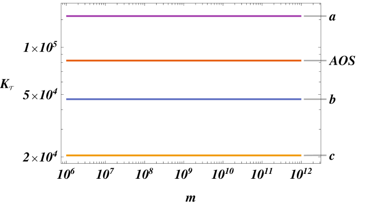
Figure 1: The Kretschmann scalar $K_{\cal{T}}$ evaluated at the transition surface vs the mass parameter $m$ for different choices of ($\delta_{b},\delta_{c}$). The Lines a, b and c correspond, respectively, to the choices $(\alpha_{b},\alpha_{c})=\{(1.97,3);\;(2,0.5);\;(1,1)\}$. The Line AOS corresponds to the choice of Eq.(III.2.1).

To see how $K_{\cal{T}}$ depends on the powers of $m$ appearing in $\delta_{b}$ and $\delta_{c}$, let us consider the case

$$\delta_{b}=\alpha_{b}\left(\frac{\ell_{p}}{m}\right)^{\beta_{b}},\quad L_{o}\delta_{c}=\alpha_{c}\left(\frac{\ell_{p}}{m}\right)^{\beta_{c}},$$ (3.29)

where $\beta_{b}$ and $\beta_{c}$ are other two arbitrary constants. In particular, in Fig. 2 we choose

$$\left(\delta_{b},\delta_{c}\right)=\left(\delta^{\text{(AOS)}}_{b},\frac{1}{{2L_{o}}}{\left(\frac{\gamma\Delta^{3/2}}{4\pi^{2}m}\right)^{1/2}}\right).$$ (3.30)

From this figure we can see that now $K_{\cal{T}}$ increases as $m$ is increasing. On the other hand, in Fig. 3, we consider the case

$$\left(\delta_{b},\delta_{c}\right)=\left(\left(\frac{\sqrt{\Delta}}{\sqrt{2\pi}\gamma^{2}m}\right)^{1/2},\delta^{\text{(AOS)}}_{c}\right),$$ (3.31)

from which we can see that $K_{\cal{T}}$ is also increasing as $m$ increases.

In addition, if $\beta_{b,c}<1/3$, then $K_{\cal{T}}$ will be decreasing as $m$ increases and when $\beta_{b,c}>1/3$, $K_{\cal{T}}$ increases as $m$ increases. To show these properties, in Fig. 4, we plot the case

$$\left(\delta_{b},\delta_{c}\right)=\left(\left(\frac{\sqrt{\Delta}}{\sqrt{2\pi}\gamma^{2}m}\right)^{1/2},\frac{1}{{2L_{o}}}{\left(\frac{\gamma\Delta^{3/2}}{4\pi^{2}m}\right)^{1/2}}\right),~{}~{}~{}~{}~{}$$ (3.32)

denoted by Line f, and the one

$$\left(\delta_{b},\delta_{c}\right)=\left(\left(\frac{\sqrt{\Delta}}{\sqrt{2\pi}\gamma^{2}m}\right)^{1/4},\frac{1}{{2L_{o}}}{\left(\frac{\gamma\Delta^{5/2}}{4\pi^{2}m}\right)^{1/4}}\right),~{}~{}~{}~{}~{}$$ (3.33)

denoted by Line g.

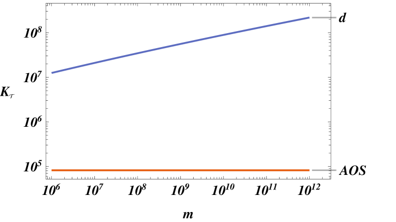
Figure 2: Plot of $K_{\cal{T}}$ vs $m$ for the choice of ($\delta_{b},\delta_{c}$) given by Eq.(3.30) with $\left(\beta_{b},\beta_{c}\right)=\left(1/3,1/2\right)$. To compare with the AOS choice, Eq.(III.2.1), the corresponding line is also plotted out, denoted by AOS.

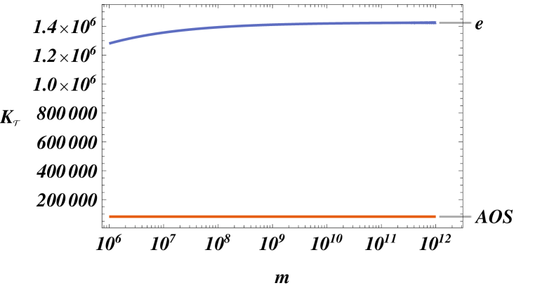
Figure 3: Plot of $K_{\cal{T}}$ vs $m$ for the choice of Eq.(3.31) with $\left(\beta_{b},\beta_{c}\right)=\left(1/2,1/3\right)$. The AOS choice, Eq.(III.2.1), corresponds to the Line AOS.

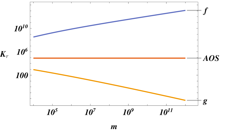
Figure 4: Plot of $K_{\cal{T}}$ vs $m$. Line f corresponds to the choice of Eq.(3.32) with $\left(\beta_{b},\beta_{c}\right)=\left(1/2,1/2\right)$, and Line g to the choice of Eq.(3.33) with $\left(\beta_{b},\beta_{c}\right)=\left(1/4,1/4\right)$.

From these figures it is clear that $K_{\cal{T}}$ will be independent of the mass parameter $m$, as long as $\delta_{b,c}$’s are all proportional to $m^{-1/3}$, no matter what the coefficients $\alpha_{b,c}$’s will be. The AOS choice is only a point on the 2-dimensional plane spanned by $\left(\alpha_{b},\alpha_{c}\right)$, given by Eq.(III.2.1). At any point of this plane, $K_{\cal{T}}$ will not depend on the choice of $m$. On the other hand, outside of this plane, that is, as long as $\beta_{b}\not=1/3$ and/or $\beta_{c}\not=1/3$, $K_{\cal{T}}$ will depend on $m$.

In [38, 30], $\delta_{b}$ and $\delta_{c}$ were uniquely determined by requiring that the physical areas of the plaquettes $\Box(\theta,\phi)$ and $\Box(x,\phi)$ at the transition surface be equal to the area gap $\Delta$. A natural question to ask is: do there exist other conditions that can uniquely determine $\delta_{b}$ and $\delta_{c}$? Our above considerations show that requiring that $K_{\cal{T}}$ be independent of the mass parameter $m$ only uniquely fixed $\beta_{b}$ and $\beta_{c}$, but not their amplitudes $\alpha_{b}$ and $\alpha_{c}$. If we further require that the masses of the BH and WH be equal, can we uniquely determine the amplitudes $\alpha_{b}$ and $\alpha_{c}$? To answer these questions, let us turn to consider the radii of the BH and WH horizons.

III.2.2 Properties of Spacetime near WH/BH horizons

The geometric radii of the WH and BH horizons are given by $r_{A}=\sqrt{p_{c}(T_{A})}$, where $T_{A}$ denotes the location of the horizon $A$. In Fig. 5, we plot the ratio between the two radii for the choices of $\delta_{b}$ and $\delta_{c}$, given by Eqs.(3.32) and Eqs.(3.33), denoted respectively by Line $x$ and $y$. Line AOS corresponds to the AOS choice.

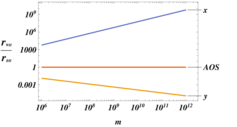
Figure 5: Plots of the ratio $r_{\text{WH}}/r_{\text{BH}}$ vs the mass parameter $m$. The lines $x$, AOS and $y$ correspond to the choices of ($\delta_{b},\delta_{c}$), given respectively by Eqs.(3.32), (• ‣ I) and (3.33).

On the other hand, from Eqs.(II.1) and (II.1), we find that $r_{\text{BH}}=r_{\text{WH}}$ implies that

$$L_{o}\delta_{c} =\frac{8m}{\gamma}\left(\frac{\sqrt{\gamma^{2}\delta_{b}^{2}+1}-1}{\sqrt{\gamma^{2}\delta_{b}^{2}+1}+1}\right)^{{2}/{\sqrt{\gamma^{2}\delta_{b}^{2}+1}}}.$$ (3.34)

Substituting Eq.(3.27) into the above equation, we find that for massive BHs

$$\alpha_{c}=\left(\frac{\gamma^{3}\ell_{p}}{2}\right)\alpha_{b}^{4}.$$ (3.35)

Therefore, imposing the conditions: a) $K_{\cal{T}}$ be independent of $m$, and b) $r_{\text{BH}}=r_{\text{WH}}$, the two parameters $\delta_{b}$ and $\delta_{c}$ can be uniquely determined by Eqs.(3.27) and (3.35), modulated a free parameter $\alpha_{b}$. In other words, there exits a family of choices of $\delta_{b}$ and $\delta_{c}$, for which the above kinds of properties are true.

IV Conclusions

In this paper, we have systematically studied the most general solutions of LQBHs of the effective Hamiltonian obtained from its classical counterpart by the replacements (1.1), with $\delta_{b}$ and $\delta_{c}$ being arbitrary constants. These solutions usually contain five free parameters, three are the integration constants of the dynamical equations [29], and two are the polymerization parameters $\delta_{b}$ and $\delta_{c}$. However, using the gauge freedom (2.3), one of them can be gauged away simply by the replacement, $T\rightarrow T+\hat{T}_{o}$, as shown explicitly by Eqs.(2.20) - (2.22). Therefore, there are generically only four free parameters, $c_{o}$, $m$, $\delta_{b}$ and $\delta_{c}$. These solutions were already studied by several authors from different aspects, including Refs. [29, 24, 30].

However, our current studies are different from those previous ones in the sense that we have also taken $\delta_{b}$ and $\delta_{c}$ as free parameters and explored their effects on various properties of the LQBH spacetimes. On the other hand, in [24] Corichi and Singh studied the solutions with the choice (2.30), while in [30, 29] the choice (• ‣ I) was adopted.

The four-parameter solutions are usually obtained in the KS spacetime, as shown explicitly by Eqs.(2.24) and (II.1), which becomes singular at both of the WH and BH horizons. Therefore, extensions beyond these horizons are needed, in order to study the asymptotic properties of the spacetimes. We have carried out such analytical extensions in Sec. II.D. Since the extensions are analytical, they are also unique. Once these are done, we are allowed to study the spacetimes in each of the three regions separately, the two asymptotic regions outside of the WH and BH horizons, and the internal region in between them.

Since the two asymptotic regions have quite similar properties, it is sufficient to study only one of them, which we choose the one in the BH side with $T>0$ [cf. Sec. III.A.1]. For any given four free parameters ($c_{o},m,\delta_{b},\delta_{c}$), the Kretschmann scalar in the asymptotic limit always takes the form of Eqs.(3.7) and (III.1.1). From these expressions it can be seen that the leading order is $1/r^{4}$, as long as $\delta_{b}\not=0$, irrespective to any specific values of the four parameters. On the other hand, when $\delta_{b}=0$, for which we have $b_{o}=1$, it reduces to its classical value, $K_{\text{GR}}=48m^{2}/r^{6}$. However, more careful analysis showed that the $r^{-4}$ terms becomes dominant over the $r^{-6}$ term only when $r>r_{c}$, where $r_{c}$ is defined by Eq.(3.9). In addition, we also show that the $r^{-4}$ term dominates over the $r^{-5}$ term only when $r>r_{c_{4}}$ given in Eq.(III.1.1). And we further show that $r^{-5}$ is dominant over $r^{-6}$ term only when $r>r_{c_{5}}$ also given in Eq.(III.1.1). For both the AOS and CS choices, we found that $r_{c}$, $r_{c_{4}}$ and $r_{c_{5}}$ are greater than $L_{\text{obs}}$ for solar mass BHs, where $L_{\text{obs}}\;(\simeq 4.4\times 10^{28}\;{\text{cm}})$ denotes the size of our observational Universe. Therefore, in both cases the asymptotic behavior of the spacetime can be well described by its classical limit ($K\simeq r^{-6}$) within our observational Universe.

We have further calculated the Hawking temperature of the BH and found that it is given by Eqs.(3.22) and (3.23). For macroscopic BHs, the gravitational fields near the BH horizons are very weak, and we expect that the temperature should be very close to that of classical BH. With this requirement, it is clear that the free parameter $c_{o}$ must be chosen so that Eq.(3.24) holds, i.e.

$$c_{o}=\frac{\gamma L_{o}\delta_{c}}{8m}.$$ (4.1)

It is remarkable to note that this was precisely the choice adopted in [24, 30].

To explore the effects of the polymerization parameters $\delta_{b}$ and $\delta_{c}$, we have first studied the Kretschmann scalar $K_{\cal{T}}$ at the transition surface $T=T_{\cal{T}}$, and found that it is independent of the mass parameter $m$ as long as they take the forms given by Eq.(3.27) for any chosen values of $\alpha_{b}$ and $\alpha_{c}$, as shown explicitly in Fig. 1. Clearly, the AOS choice of Eq.(III.2.1) is only a point in the plane spanned by ($\alpha_{b},\alpha_{c}$). To see how $K_{\cal{T}}$ depends on the powers of $m$ in the expressions of $\delta_{b}$ and $\delta_{c}$, we have studied the more general forms Eq.(3.29), and found that $\beta_{b}=\beta_{c}=1/3$ is the unique choice that leads $K_{\cal{T}}$ to be independent of $m$, as shown explicitly by Figs. 2 - 4.

Finally, we have also explored the condition at which the WH and BH masses are equal, and found it is given by Eq.(3.34). If we further require that the Kretschmann scalar at the transition surface be independent of $m$, we find that $\delta_{b}$ and $\delta_{c}$ must take the form (3.27) with $\alpha_{c}$ being given by Eq.(3.35). Therefore, it is concluded that as long as $\delta_{b}$ and $\delta_{c}$ are chosen as

$$\delta_{b}=\alpha_{b}\left(\frac{\ell_{p}}{m}\right)^{1/3},\;\;L_{o}\delta_{c}=\alpha_{b}^{4}\left(\frac{\gamma^{3}\ell_{p}}{2}\right)\left(\frac{\ell_{p}}{m}\right)^{1/3},~{}~{}~{}~{}$$ (4.2)

the corresponding LQBHs shall have the same desired properties as those of the AOS solution [30], for any given non-zero and positive $\alpha_{b}$.

With the choice of $\delta_{b}$ and $\delta_{c}$ given by Eq.(4.2), an interesting question is: is it possible to impose any constraint on the choice of the free parameter $\alpha_{b}$ from observations? As the Event Horizon Telescope (EHT) just observed two supermassive BHs, one is the $M87^{*}$ BH located at the center of the more distant Messier 87 galaxy [3], and the other is the Sagittarius $A^{*}$ BH located at the center of our own Milky Way galaxy [58], it would be very interesting to see the effects of $\alpha_{b}$ on the shadows of supermassive BHs. In Fig. 6, we plot the dependence of $r_{c}$ on $\alpha_{b}$ for a solar mass, Sagittarius $A^{*}$ and $M87^{*}$ BHs, respectively, from which it can be seen that $r_{c}$ becomes very small, so that the quantum effects are expected to be large, only when $\alpha_{b}$ is very large. For more details, we would like to come back to this issue in another occasion, as such considerations clearly are out of the scope of the current paper.

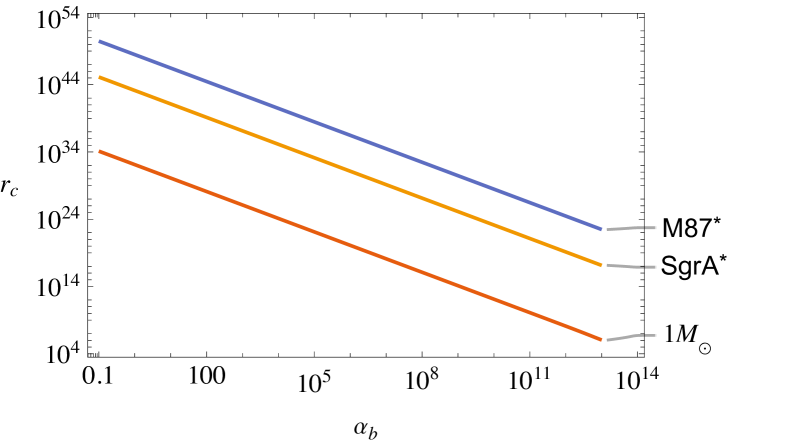
Figure 6: Plots of the critical radius $r_{c}$ vs $\alpha_{b}$ for a solar mass, Sagittarius $A^{*}$ and $M87^{*}$ BHs, respectively.