Now and Future of Artificial Intelligence-based Signet Ring Cell Diagnosis: A Survey

Abstract

Since signet ring cells (SRCs) are associated with high peripheral metastasis rate and dismal survival, they play an important role in determining surgical approaches and prognosis, while they are easily missed by even experienced pathologists. Although automatic diagnosis SRCs based on deep learning has received increasing attention to assist pathologists in improving the diagnostic efficiency and accuracy, the existing works have not been systematically overviewed, which hindered the evaluation of the gap between algorithms and clinical applications. In this paper, we provide a survey on SRC analysis driven by deep learning from 2008 to August 2023. Specifically, the biological characteristics of SRCs and the challenges of automatic identification are systemically summarized. Then, the representative algorithms are analyzed and compared via dividing them into classification, detection, and segmentation. Finally, for comprehensive consideration to the performance of existing methods and the requirements for clinical assistance, we discuss the open issues and future trends of SRC analysis. The retrospect research will help researchers in the related fields, particularly for who without medical science background not only to clearly find the outline of SRC analysis, but also gain the prospect of intelligent diagnosis, resulting in accelerating the practice and application of intelligent algorithms.

,,,,,

[a]organization=School of Artificial Intelligence,addressline=Beijing University of Posts and Telecommunications, city=Beijing, postcode=100876, country=China [b]organization=Department of Pathology, School of Basic Medical Sciences,addressline=Peking University Third Hospital, city=Beijing, postcode=100191, country=China

Research highlight 1

Research highlight 2

1 Introduction

Signet ring cells (SRCs) reflect special histopathological features where nuclei are squeezed into eccentrically placed crescent shapes by abundant intracellular mucins [9]. Histopathologically, SRC carcinoma is noted when more than 50% tumor cells contain SRC features, while tumors with few SRC components are also concerned [9]. Although the majority of SRC carcinomas occur in the gastrointestinal tract, they also appear in esophagus, lung, pancreas, appendix, gallbladder, breast, urinary bladder, ovary, prostate, skin, and other tissues [117, 118, 34, 7, 59]. When gastric SRC carcinoma is diagnosed, it is aggressive and can be accompanied by diffuse growth of adenocarcinoma cells and extensive connective tissue proliferative response [98], especially when infiltrating into the layers of submucosa, muscularis propria or serosa. SRC features are associated with high peripheral metastasis rate, poor response to neoadjuvant treatment, and particular dismal survival [117, 118, 54, 104, 66, 81, 137]. SRCs will not aggregate to form a relatively regular structure, thereby they are difficult to identify in low magnification pathological diagnosis, while the cell morphology in high magnification pathological images is very similar to plasma cells, intestinal metaplasia, and activated endothelial cell [21]. Therefore, SRCs are easily missed even for experienced pathologists. As a result, computer-aided algorithms are expected to assist pathologists to improve the screening speed and accuracy of SRCs.

Since artificial intelligence (AI) has made remarkable achievements in natural image processing such as classification, segmentation, and detection [8, 160, 96], more and more clinically effective medical image processing algorithms based on convolutional neural networks (CNNs) have emerged [119, 84, 106, 63]. Actually, the automatic diagnosis of SRCs has been concerned since 2008, where a deep learning network, LeNet [69], was combined with color features to detect SRCs [94]. However, the automatic screening algorithms have not made a greater breakthrough until recent years. Different from normal cells and other tumor cells, the distributions of SRC are various, which leads to the difficulty for the algorithms to capture typical features. And thus, SRC-related data were often ignored or removed in some deep learning-based lesion screening tasks. For example, Cowan et al. excluded slides suggestive of SRC carcinoma because these entities performed poorly in their training data [42]. Although the Lizard Dataset contained nearly half a million labeled nuclei in hematoxylin and eosin (H&E) stained colon tissue, SRCs were not involved and expressed particular interest in future work [35]. Actually, SRCs have gradually received attention in recent years. SRC carcinoma was often mixed in the automatic identification of whole-slide images (WSIs) as one of the subtypes, and was often analyzed as typical cases [100, 91, 6, 1]. However, many studied suggested that the sensitivity of identifying SRC lesions was significantly lower than that of well-differentiated adenocarcinoma without SRCs [143, 60, 45, 119, 50, 127]. Therefore, more attention needs to be paid to the recognition of SRCs, which was indeed concerned in the discussions of some articles [74, 52, 10, 121, 28, 26, 36]. Particularly, the DigestPath dataset [22] was released to encourage typical SRCs detection in histopathology image patches.

We observe that there has been a representative and wide-ranging survey for AI-based medical image processing [79], especially for microscopy and histopathology images [120, 145, 85, 46, 3, 142]. In addition, surveys of AI algorithms for identification for different tissues and organs were also emerged, including brain [88], lung [141], cervix [105], colorectum [146], skin [24], and liver [5]. However, SRCs were overlooked in these reviews. Therefore, this paper summaries most of the AI-related articles for SRC identification until August 2023 to help researchers comprehensively understand this field.

The remainder of this paper is organized as follows. Section 2 presents the overview of problem description, public SRC datasets (the corresponding evaluation metrics are summarized in the Supplementary Materials), and the challenges of automatic diagnosis for SRCs. Section 3 illustrates the AI-based methodology for SRC identification, which is categorized into pre-processing (Section 3.1), classification (Section 3.2), detection (Section 3.3), and segmentation (Section 3.4). Section 4 discusses the limitations of existing algorithms and the future trends for clinically accurate SRC identification with AI assistance. Section 5 provides the conclusions of this paper.

2 Overview

2.1 Problem description

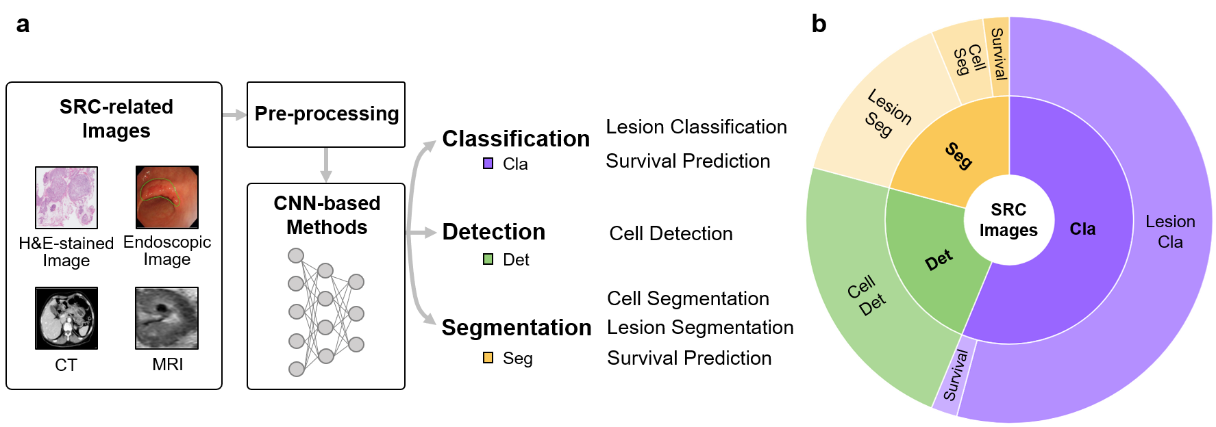
Figure 1: An overview of the SRC diagnosis driven by deep learning. (a) The features of SRC-related images are captured through CNN-based methods after pre-processing. These methods can be divided into three tasks, i.e., classification, detection, and segmentation which correspond to different diagnostic sub-tasks. (b) The statistical proportion of the academic articles included in this survey for each task and sub-task.

Apart from a particular study on single-shot femtosecond stimulated Raman scattering [87], most SRC diagnosis algorithms were carried out based on four types of images (Fig. 1), namely, H&E stained WSIs, computed tomography (CT), magnetic resonance imaging (MRI), and endoscopic images. Since histopathological images at high magnification clearly show the morphology of nuclei and cytoplasm after staining, the automatic algorithms of SRCs based on H&E stained WSIs are notably more than the other three types. Following the natural image analysis pipelines with high-performance, the SRC diagnosis algorithms can also be divided into three categories: classification, detection and segmentation.

Classification: For classification, the goal is to train a model $f_{\theta}$ to predict the class label of an arbitrary test sample (e.g., a WSI or a patch). Specifically, in supervised learning, we define the training set as $Tr=\left(x_{tr}^{\left(i\right)},y_{tr}^{\left(i\right)}\right)_{i=1}^{N_{tr}}$, where $N_{tr}$ is the total number of training samples. For each sample, $x_{tr}^{\left(i\right)}\in R^{C_{h}\times H\times W}$ denotes the image to be classified with a resolution of $H\times W$ and $C_{h}$ channels, and $y_{tr}^{\left(i\right)}\in\ R^{C_{l}}\$ denotes the ground-truth annotation with $C_{l}$ categories. Binary classification is the most common scenario for SRC diagnosis, where SRCs are usually regarded as positive samples. For instance, to predict whether a patch of WSIs contains tumors, the label is set to 1 for a positive case and 0 for a negative one. During the training process, a classification model $f_{\theta}$ is trained with the training set $Tr$ based on a specific loss function $L$. For inference process, the trained model provides the prediction $p_{te}^{\left(i\right)}$ for each sample $x_{te}^{\left(i\right)}$ in the test set. In addition, the parameters pretrained on large-scale datasets and slide-level annotations are also leveraged for other training strategies, such as transfer learning and weakly supervised learning. The details of SRC-related classification algorithms are elaborated in Section 3.2.

Detection: In object detection, the model $f_{\theta}$ is trained to perform both object localization and classification. Therefore, the given annotations are modified as $y_{tr}^{\left(i\right)}=\left(b_{j}^{\left(i\right)},c_{j}^{\left(i\right)}\right)_{j=1}^{M_{i}}$, where $b_{j}^{\left(i\right)}$ represents the position and size of the $j$th object’s bounding box in the $i$th image, while $c_{j}^{\left(i\right)}$ contributes its category, and $M_{i}$ represents the number of objects in this image. In SRC diagnosis, the aim is to train a detector $f_{\theta}$ with a classification loss $L_{cla}$ and a regression loss $L_{reg}$, which can accurately locate the SRCs in the test set. Besides, semi-supervised learning strategy (see Section 3.3) is also applied to handle the incomplete labeling problem of the SRC detection.

Segmentation: This task aims to achieve pixel-level dense prediction instead of simple classification of images. More formally, the ground-truth mask of training data is defined as $y_{tr}^{\left(i\right)}={(y_{j}^{\left(i\right)})}_{j=1}^{H\times W}$, where $y_{j}^{\left(i\right)}$ is the $j$th pixel-level annotation of the $i$th image, and the number of pixels is $H\times W$. For pathological images, the trained model $f_{\theta}$ is expected to generate reliable masks with densely predicted labels, on which sub-tasks can be performed such as survival prediction, lesion localization and cell segmentation. In addition to fully supervised learning, training strategies such as weakly supervised learning, collaborative learning and multi-task learning have also been introduced due to the lack of suitable dense annotations, which are illustrated in Section 3.4.

2.2 SRC datasets

According to the articles covered in this survey, both public and private datasets were enrolled in SRC automatic diagnostic tasks. Among them, two public datasets DigestPath [22] and The Cancer Genome Atlas (TCGA) were most frequently adopted.

2.2.1 DigestPath dataset

DigestPath was a dataset from Digestive-System Pathological Detection and Segmentation Challenge 2019, which was the first public dataset for object detection of SRCs. It was applied to SRC automatic diagnosis of classification [52, 10], detection [155, 148, 76, 37], and segmentation [74, 21, 158]. The training set was collected from two organs, i.e., intestinal and gastric mucosa, and was divided into positive and negative subsets. The positive one consisted of 77 pathological images cropped from 20 WSIs, which contained SRCs annotated with bounding boxes by experienced pathologists. The negative one consisted of 378 images from 79 WSIs with on SRCs, but may contain other types of tumor cells. The sizes of the negative images were ($2000px\times 2000px$), while the positive ones were slightly larger but not fixed. Note that due to the tedious process of manual labeling, there existed a considerable part of SRCs left unlabeled in the positive set, which may introduce noises to some tasks. Besides, DigestPath contained a still unavailable test set with 227 images from 56 patients, in which 27 images from 11 patients were positive ones. All H&E stained WSIs involving in the DigestPath dataset were captured at 40$\times$ magnification.

2.2.2 TCGA dataset

TCGA program was first launched in 2006 by the National Cancer Institute (NCI) and the National Human Genome Research Institute (NHGRI) of the US. It aimed to comprehensively study the genomic alterations in all major cancers to make outstanding contributions to cancer prevention, diagnosis and treatment. Over the past ten years, more than 20,000 biological samples were collected, covering 33 cancer types with 10 rare ones. TCGA provided abundant representative H&E diagnostic WSIs. The TCGA Stomach Adenocarcinoma (STAD), Colon Adenocarcinoma (COAD) and Rectum Adenocarcinoma (READ) were popular cohorts in SRC-related classification tasks. On the basis of these data, novel deep learning models to classify the tissue / non-tissue, differentiation grades, and sub-types of tumors were developed [60, 48, 50, 71, 49]. Although we could find SRC related cases in different subsets of TCGA, there was still a lack of systematic integration of SRC cases.

2.3 Challenges of automatic SRC diagnosis

2.3.1 Biological characteristics

Different from normal cells grown in an organized manner forming specific structures, SRCs are low adhesive with uncertain distribution. Histopathologically, SRCs may be clustered or isolated. At low magnification, the isolated SRCs are easily missed by pathologists and algorithms due to the small size. At high magnification, unlike most other tumor cells with convex shapes, the nuclei of SRCs are squeezed into an irregular crescent shape by intracellular proteins. The uncertainty of the squeezing power leads to the diversity of nucleus morphology, and the flooding of intracellular proteins affects the accurate discrimination of cell boundaries. In addition, SRCs are easily confused with ice crystal bubbles in intraoperative frozen slices. This leads to the difficulty in evaluating whether there are SRCs in the surgical margin tissues or whether there are SRCs metastasis in the omentum and other tissues. Therefore, the recognition of SRCs is challenging for both pathologists and algorithms at multi-scale magnification.

2.3.2 Image quality

Different acquisition equipment and conditions have a great impact on the quality of H&E stained WSIs, CT, MRI and endoscopic images. Take the H&E stained WSIs which are usually adopted to confirm the existence of SRCs as examples, the nuclei and cytoplasm are stained into blue and red, and the intracellular proteins are hardly stained. On the one hand, the color distribution of images will be greatly affected by the dyeing process of different batches, concentrations and laboratory environments. On the other hand, the angle and thickness of tissue segmentation, the rupture and overlap of tissue, and other external factors will affect the appearance of cells. In addition, different digital scanners will show different brightness and saturation for the same WSI. Parameters such as focal length during scanning will affect the clarity of WSIs. Therefore, these uncontrolled factors introduce a lot of noises to the SRC image distribution, which puts forward high requirements for the robustness of AI algorithms.

2.3.3 Manual annotations

Accurate annotations are of great benefit to the accuracy improvement of AI algorithms, while rough annotations are bound to restrict the performance of models due to noise interference. In fact, since SRCs are difficult even for experienced pathologists to identify without omission, the manual labeling of SRCs requires high professionalism. In addition, pixel-wise labeling is time-consuming and labor-intensive, which further limits the scale of accurate annotations. Usually, pathologists only annotate the cells that are confirmed to be the positive SRC samples, which leads to incomplete labeling in the images. In this situation, if all unmarked areas are regarded as non-SRCs, a large number of SRC noises will be mixed into the negative samples, which will confuse the convergence of the models. In most cases of practical applications, medical centers can only provide patient-level or image-level annotations for algorithm learning, which limits the use of high-performance fully supervised algorithms and weakly supervised algorithms like multiple instance learning (MIL) [27] are required.

2.3.4 Sample imbalance

The data distribution has a great influence on the model fitting of deep learning. When the quantities of positive and negative samples in the training set are unbalanced, the model will tend to predict the tested samples to be the category with more training samples, so as to minimize the value of the loss function. When the data distribution of the test set is similar to that of the training set, although the biased the model will make the overall evaluation metrics look satisfactory, it will sacrifice the accuracy of few-shot categories, resulting in an intolerable problem of missed detection in clinical practice. In fact, sample imbalance in SRC automatic diagnosis task is common. First, the patient-level samples are imbalanced, since SRC-related patients are far fewer than normal people. Second, the cell distributions are imbalanced. In a screening image, SRCs account for a limited proportion of tissues, while other cells occupy a large area. Third, although SRCs have typical morphological characteristics, the differences among patients, organs, and the image collection process will still introduce disturbances, leading to uncertainty and imbalance of the difficulty of intra class samples. Therefore, to ensure the fairness of the model in SRC automatic diagnosis, the sampling strategy and data augmentation were usually introduced to control the number of samples of different categories in the training set to be similar. In addition, some loss functions were specially designed to increase the loss weights of few-shot samples to force the model to focus on the SRCs. In natural image processing, the long-tailed learning [86] was specially proposed to focus on the widespread sample imbalance issue. However, long-tailed learning has not been embedded in the existed SRC-related studies, since SRC automatic diagnosis task involved fewer categories than natural image processing.

3 Methodology

This section presents a general reference for SRC diagnostic methods. As shown in Fig. 1, existing works cover four types of SRC-related images, i.e., H&E stained, endoscopic, CT, and MRI images. After pre-processing designed according to the type characteristics, the high-dimensional features of the target images are captured by the CNN-based methods, which can be roughly divided into three categories, i.e., classification, detection and segmentation, corresponding to different detailed tasks.

3.1 Pre-processing

Data pre-processing is commonly required for CNNs to extract robust features, which significantly affects the performance of the models. Considering the variance of purposes, we summarize the pre-processing methods into the categories including image normalization, denoising, foreground or regions of interest (RoIs) extraction, data augmentation, and others. The details of pre-processing for each article are listed in Table LABEL:table:Pre.

Table 1: Summary of data pre-processing and augmentation for SRC-related algorithms (Only the pre-processing mentioned in the articles are included).

Publication	Year	Task	Modality	Pre-processing
				Image normalization	Denoising	Foreground (RoI) extraction & background removal	Data augmentation	Others
[149]	2019	Classi-fication	Endo-scopic images	Mean value (from ImageNet dataset) subtraction	/	/	Random flipping, small rotation, elastic deformation, kernel erosions, and dilations	/
[97]	2019	Classi-fication	H&E	/	/	/	Slight shear / zoom, flipping, whitening	/
[60]	2020	Classi-fication	H&E	/	Gaussian blur smoothing	Thresholding on RGB values	/	/
[122]	2020	Object detection	H&E	/	/	/	Color jitters, horizontal and vertical flipping	/
[140]	2020	Object detection	H&E	/	/	/	Random flipping	/
[119]	2020	Segmen-tation	H&E	/	/	Otsu thresholding on grayscale image	Random rotations by $90\,{{}^{\circ}}$, $180\,{{}^{\circ}}$, and $270\,{{}^{\circ}}$, flipping, Gaussian and motion blurs, color jitters	/
[82]	2021	Classi-fication	MRI	Z-score	/	/	/	/
[53]	2021	Classi-fication	H&E	/	/	Otsu thresholding on a grayscale version	/	/
[103]	2021	Classi-fication	H&E	Stain normalization	/	/	CIELAB color space augmentation	/
[20]	2021	Classi-fication	H&E	/	/	/	Flipping, random rotation, translation, contrast, brightness, hue, saturation	/
[48]	2021	Classi-fication	H&E	Color normalization	/	CNN-based classifier	Random rotations by $90\,{{}^{\circ}}$, random horizontal and vertical flipping	/
[71]	2021	Classi-fication	H&E	Color normalization	/	CNN-based classifier	Random rotations by $90\,{{}^{\circ}}$, random flipping, perturbation of the contrast and brightness	/
[52]	2021	Classi-fication	H&E	/	/	Otsu thresholding	Filpping, $90\,{{}^{\circ}}$ rotations, translations, color shifts	/
[107]	2021	Classi-fication	H&E	/	/	/	Rotations of $90\,{{}^{\circ}}$, $180\,{{}^{\circ}}$, $270\,{{}^{\circ}}$	/
[10]	2022	Classi-fication	H&E	Stain normalization	Median blur, Gaussian blur	SLIC	Random rotation	/
[50]	2021	Classi-fication & segmentation	H&E	Macenko stain normalization	/	Foreground segmentation based on U-Net	/	/
[151]	2021	Classi-fication & segmentation	H&E	/	/	Color deconvolution and Otsu thresholding	Flipping, rotation, random cropping and resizing, changes of the aspect ratio and image contrast, Gaussian noise	/
[76]	2021	Object detection	H&E	/	/	/	Flipping and rotation	/
[18]	2021	Object detection	H&E	/	/	/	Random flipping	/
[123]	2021	Object detection	H&E	/	/	/	Color jitters, flipping	/
[155]	2021	Object detection	H&E	/	/	/	Random flipping, data normalization (with a label correction model)	USRNet (to obtain low-resolution images)
[73]	2022	Segmen-tation	CT	Z-score	/	/	Random rotation, flipping, cropping	Resampled with isotropic spacing, clipped intensity values, wavelet filtering
[21]	2022	Segmen-tation	H&E	/	/	A coarse U-Net	/	/
[134]	2022	Classi-fication	H&E	/	/	Otsu thresholding	Brightness, contrast, hue, and saturation modified, JPEG artifacts	/
[49]	2022	Classi-fication	H&E	/	/	/	Hue and saturation shifts, flipping, rotation, and random erasing	/
[68]	2022	Classi-fication	H&E	/	/	/	Flipping, rotation, color changes, and blurring	/
[1]	2022	Classi-fication & segmentation	H&E	Color normalization	/	Otsu thresholding in H and S channels of HSV color space	Random cropping, rotation, flipping, and color changes	/
[130]	2022	Segmen-tation	H&E	/	/	/	Changes of 30% for hue, 0.4 to 1.6 for saturation, 0.7 to 1.3 for brightness, and 0.4 to 1.6 for random scaling / contrast	/
[99]	2023	Classi-fication	H&E	Stain normalization	/	/	Flipping, rotation, scaling, color jitters, Gaussian blurring and solarization	/
[67]	2023	Classi-fication	H&E	/	/	DeepLab v3+	Flipping, rotation, scale shifts, brightness, contrast, hue, saturation, Gaussian noises, elastic transforms, grid and optical distortions	/

3.1.1 Image normalization

Digital images usually have appearance differences such as intensity and color etc., thereby the accuracy of the models will decrease because of insufficient generalization ability. Image normalization is usually employed to eliminate this uncontrolled variability. It emphasizes the real discriminative features without excessive interference from external factors, and accelerates network convergence. For example, Yoon et al. performed the mean value subtraction on each channel of the endoscopic images [149]. In addition, z-score normalization is usually utilized with the corresponding mean value and standard deviation to achieve standard normal distributions [82, 73]. Notably, stain / color normalization is relatively necessary for the H&E images on account of the huge variation in stains, operators and scanner specifications. Its basic principle is to standardize the color appearance of all images to a reference image chosen by an experienced pathologist [56, 92, 108, 136]. Many SRC-related methods based on H&E stained images adopted stain / color normalization to enhance the robustness of models to the diversity of staining [103, 48, 50, 71, 10, 1, 99].

3.1.2 Denoising

Noise is inevitably embedded in the raw images. For instance, air bubbles, compression artifacts, pen marks, blurring, tissue tears and folds, and over-stained areas in H&E stained samples are irrelevant to the characteristics of SRC lesions, which should be removed to promote the quality of the inputs. Filtering algorithms can reduce the interference of some above factors. Among them, Gaussian blur [60, 10] and median blur [10] filters were commonly performed to denoise without severely blurring edges of the objects.

3.1.3 Foreground (RoI) extraction/ background removal

In H&E stained WSIs, object areas containing pathological tissues are usually small, while the blank areas which contribute little to the subsequent tasks occupy the majority. Therefore, the valid parts of WSIs are required to be extracted as the RoIs, and the background needs to be removed. The most direct way to obtain the foreground quickly was to convert the colored images to binary ones [60, 53, 151, 52, 119, 134, 1]. It leveraged the difference in grayscale between the foreground and background at low magnification, and identified each pixel through a reasonable threshold. Otsu [101] was the most popular binarization method, which automatically determined the adaptive thresholds by maximizing the inter-class variance in a variety of SRC tasks. In addition, the tissue / non-tissue regions could also be distinguished by CNN-based approaches. For example, CNNs were used as classifiers to choose proper tissue patches for subsequent tumor classification [48, 71]. Besides, segmentation networks such as U-Net [110] and DeepLab v3+ [14] were adopted to outline the foreground [50, 21, 67]. Compared with the traditional methods based on binarization, the CNN-based methods could flexibly extract specific RoIs according to requirements, but they also introduced additional time cost.

3.1.4 Data augmentation

Data augmentation techniques can expand the training set based on existing data, and thus improve the robustness and generalization of models with overfitting minimized. In SRC classification, detection and segmentation, spatial and color transformations were commonly employed. The spatial transformations for SRC diagnosis included horizontal and vertical flipping, rotation, elastic deformation, erosion, dilation, cropping, resizing, and translation [149, 48, 71, 151, 52, 107, 10, 97, 20, 73, 119, 155, 76, 122, 140, 18, 123, 49, 68, 1, 99, 67]. The color transformations involved CIELAB color space augmentation, superimposed Gaussian noise, whitening, Gaussian blur, motion blur, color shifts, and color jitters including fluctuation of contrast, brightness, hue, and saturation [103, 71, 151, 52, 97, 20, 119, 122, 123, 134, 49, 68, 1, 130, 99, 67]. The details of data augmentation in the articles covered in this survey are illustrated in Table LABEL:table:Pre.

3.1.5 Other pre-processing

Unlike the common methods mentioned above, some pre-processing operations were related to specific tasks. For example, to obtain the hand-crafted radiomic features, Li et al. resampled each CT image with isotropic spacing in the transverse plane, and then, intensity values were clipped to the range of [-90, 170] to remove outliers [73]. Zhang et al. adopted USRNet [154] to reduce the resolution of training data, and the efficiency for SRC detection in low-resolution pathological images was demonstrated [155].

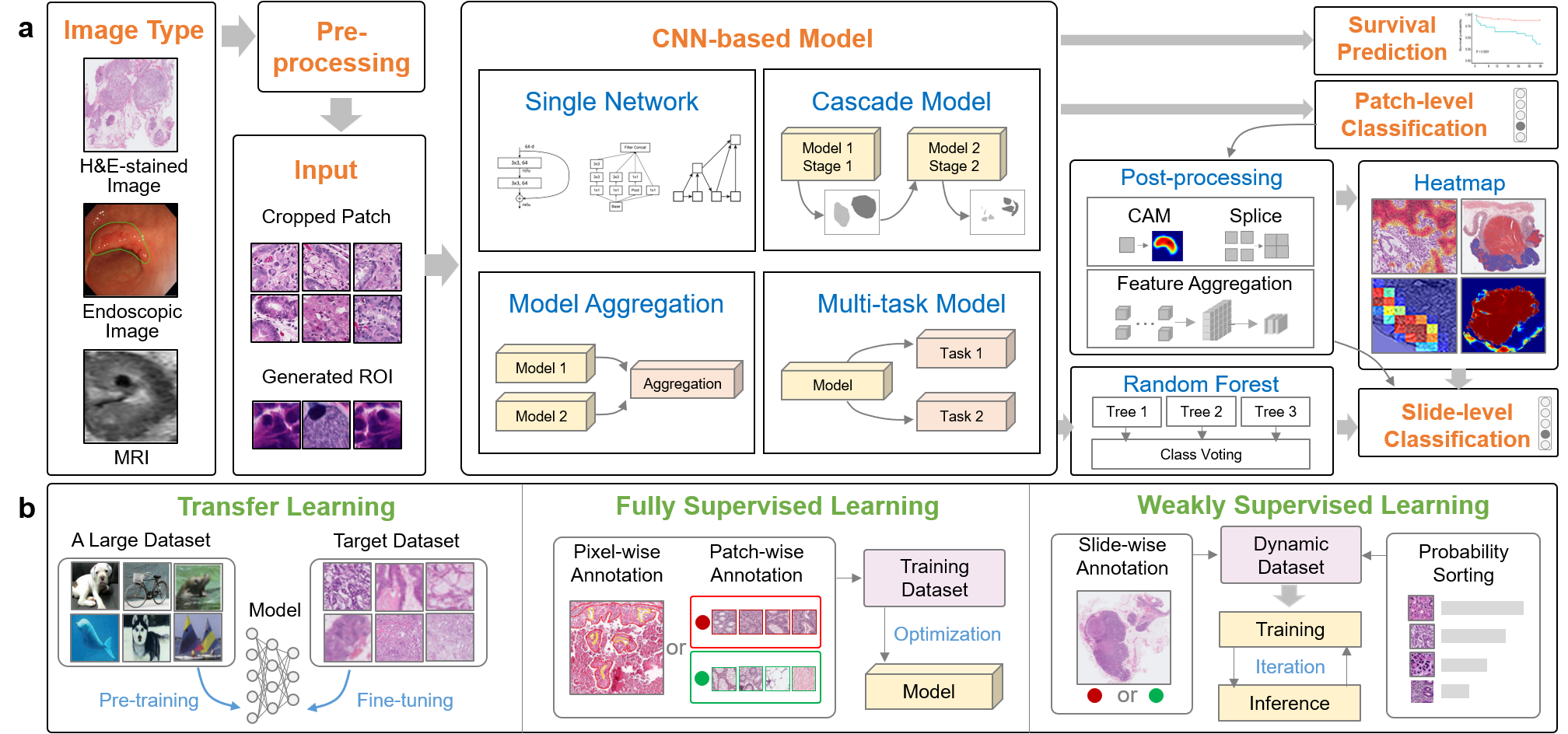
Figure 2: An overview of classification methods for SRC diagnosis. (a) The process of SRC diagnosis based on classification methods. (b) The learning strategies of SRC classification according to the articles included in this survey.

3.2 Classification

Among the classification methods, the target images were fed into the CNNs after corresponding pre-processing. As illustrated in Fig. 2, the high-dimensional features of the input images were captured through four types of CNN-based classification models. Then the features were adopted to accomplish survival prediction, patch-level prediction, or slide-level prediction. The related models were trained through different combinations of training strategies such as transfer learning, fully supervised learning, and weakly supervised learning. The overview of articles related to SRC classification is summarized in Table LABEL:table:Cla. The details of CNN-based models, task-related post-processing, and training strategies are presented next.

Table 2: Summary of automatic SRC diagnosis algorithms on the basis of classification.

Publication	Year	Modality	Target	Task	Data	Network	Loss	SRC diagnosis
[149]	2019	Endo-scopic images	Early gastric cancer	Early gastric cancer detection and depth prediction	11,539 endoscopic images from 800 patients	VGG-16	A new loss by adding Grad-CAM	The histology types of lesions consisted of well / moderately / poorly-differentiated adenocarcinoma, and SRC carcinoma.
[82]	2021	MRI	Locally advanced rectal cancer	Distant metastasis prediction by integrating deep MRI information and clinicopathologic factors	MRI from 235 patients	ResNet-18	BCE-Loss	SRC carcinoma was part of histologic variants in rectal adenocarcinoma.
[97]	2019	H&E	Gastric SRC carcinoma	Histopathologic features of the behavior of gastric SRC carcinoma	516 images from 10 cases	A 6‐layer CNN	BCE-Loss	SRCs remained within intramucosal areas with poorly differentiated components as dense neighbors.
[60]	2020	H&E	Stomach lesion	Identification of well, moderately, and poorly differentiated adenocarcinoma, poorly cohesive carcinoma, and normal gastric mucosa.	94 cases of gastroscopic biopsy specimens, and adenocarcinoma WSIs in TCGA (3 stomach and 3 colon cases)	VGG-16, Inception-v3, EfficientNet, MRD-Net [4], N-Net [114], CAT-Net [133]	MSE-Loss	The method was more accurate in well and moderately differentiated adenocarcinomas than in poorly differentiated adenocarcinomas and poorly cohesive carcinomas including SRCs.
[52]	2021	H&E	Gastric SRC carcinoma	Gastric SRC carcinoma classification via fully and weakly supervised learning	2,824 cases from two hospitals (private, $20\times$ magnification), DigestPath (public, $40\times$ magnification)	EfficientNet-B1	BCE-Loss	The lesions with aggregated SRCs had a high response, while the scattered SRCs had a low response, and the positive probability of a WSI was determined by the highest response of the patches.
[103]	2021	H&E	Gastric tumor	Automatical classification into negative for dysplasia, tubular adenoma, or carcinoma based on the method of [83]	201 cases of gastric resection and 2,233 cases of biopsy specimens for training, and 7,440 biopsy specimens for evaluation	Inception-v3 for patch classification, an aggregation CNN to generate slide features	CE-Loss	SRC carcinoma was one type of the positive targets. Despite of the overall high accuracy in classifying epithelial tumors, SRC carcinoma suffered from false negatives.
[151]	2021	H&E	Gastric cancer	Screening and localization of gastric cancer based on a multi-task CNN	10,315 WSIs collected from 4 medical centers	DLA structure combined with classification and segmentation branches	BCE-Loss	SRC carcinoma was one type of the positive targets.
[45]	2021	H&E	Gastric cancer	Lymph node quantification and metastatic cancer identification	921 WSIs from 222 patients	Xception, DenseNet-121	Not mentioned	The system correctly classified most of the patches, but was prone to misdiagnosis when the SRCs were few and scattered.
[48]	2021	H&E	Gastric carcinoma	To distinguish differentiated / undifferentiated and non-mucinous / mucinous tumor types	396 WSIs of 371 patients from TCGA for training, and 232 private WSIs for validation	Inception-v3	Not mentioned	SRC carcinoma was regarded as undifferentiated-type.
[107]	2021	H&E	Here-ditary diffuse gastric cancer	Detection of regions of hereditary diffuse gastric cancer	7 gastrectomy specimens (133 annotated tumor foci)	DenseNet-169	Not mentioned	Regions suspicious for intramucosal SRC carcinoma could be detected.
[53]	2021	H&E	Gastric diffuse-type adenocarcinoma	To classify gastric diffuse-type adenocarcinoma from other adenocarcinoma and non-neoplastic subsets	2,929 endoscopic biopsy cases of human gastric epithelial lesions	EfficientNet-B1, Inception-v3	CE-Loss	The diffuse-type consisted of poorly-differentiated and SRC carcinoma.
[50]	2021	H&E	Colon adenocarcinoma	Tumor microenvironment analysis by recognizing nine different contents	441 WSIs of 433 patients from TCGA	VGG-19	Not mentioned	The SRC was not sufficiently presented in the training set and were neglected by the model.
[71]	2021	H&E	Color-ectal cancer	Classification of tissue / non-tissue, normal / tumor, and microsatellite stable / instability	1,920 WSIs from TCGA (colon and rectal cancers) for training, and 365 private WSIs for validation	Inception-v3	CE-Loss	SRC was associated with the classification of mucinous adenocarcinoma and SRC carcinoma.
[20]	2021	H&E	Color-ectal cancer	Identification of nodal micrometastasis based on an annotation-free method [12]	3,182 WSIs from 1,051 patients	ResNet-50	BCE-Loss	The model performed well on the overall task of identifying micrometastasis and macrometastasis, but slightly worse in identifying SRC and poorly differentiated adenocarcinoma.
[10]	2022	H&E	SRC cancer	Detection of ring cell cancer based on RoIs determined by SLIC superpixels	DigestPath dataset	VGG-16, VGG-19, Inception-v3	Not mentioned	SRC gastric cancer classification was conducted after cropping the small RoIs through SLIC superpixels method.
[134]	2022	H&E	Gastric poorly differentiated adenocarcinoma	Poorly differentiated adenocarcinoma classification in gastric endoscopic submucosal dissection with weakly supervised learning	5,103 specimens (2,506 Endoscopic submucosal dissection, 1,866 endoscopic biopsy, and 731 surgical specimen)	EfficientNet-B1	BCE-Loss	SRC carcinoma was included in poorly differentiated adenocarcinoma.
[68]	2022	H&E	Gastric cancer	Epstein-Barr Virus (EBV) status prediction from pathology images of gastric cancer biopsy	137,184 patches from 16 tissue microarray (708 tissue cores), 24 WSIs, and 286 biopsy images	ResNet, MobileNet [44], EfficientNet, DeiT [132]	CE-Loss	The presence of SRC components was prone to be correlated with gastric cancer specimens without EBV.
[1]	2022	H&E	Gastric cancer	Development and multi-institutional validation of an artificial intelligence-based diagnostic system	984 patients for training and 2,771 patients for validation	GoogLeNet[125]	Not mentioned	SRC could be detected and the performance of a case of poorly cohesive adenocarcinoma with SRCs was discussed.
[90]	2022	H&E	Colorectal cancer	Microsatellite instability prediction of colorectal cancer	144 WSIs from 3 hospitals	ResNet, MobileNet, Inception, EfficientNet were embeded in the proposed PPsNet	CE-Loss	Certain histological features like SRC were significantly associated with microsatellite instability.
[49]	2022	H&E	Colorectal cancer	DNA mismatch repair status prediction based on domain adaption and MIL	441 WSIs from TCGA,78 WSIs from PAIP [57], and private WSIs (355 from surgical specimens and 341 from biopsy specimens)	DenseNet-121, IBN-net [102]	Focal Loss, CE-Loss	SRC carcinoma was one of the histology subtypes.
[87]	2022	Single-shot femtosecond stimulated Raman scattering	Gastric cancer	Instant diagnosis of gastroscopic biopsy based on single-shot femtosecond stimulated Raman histology	279 patients	Inception-ResNet-V2 [124]	CE-Loss	Mucinous adenocarcinoma and SRC carcinomas were labeled as undifferentiated cancer in this study.
[147]	2023	Endoscopic images	Gastric SRC carcinoma	Identification of gastric SRC carcinoma using few-shot learning	50 gastric benign ulcers, 50 adenocarcinoma and 50 SRC cacinoma	EfficientNetV2-S [129]	Not mentioned	Gastric benign ulcers, adenocarcinoma and SRC carcinoma could be classified through K-nearest neighbor classifier based on features from transfer learning.
[33]	2023	Endoscopic images	Gastric cancer	Cooperation between artifcial intelligence and endoscopists for diagnosing invasion depth of early gastric cancer	700 images	EfcientNet-B1	Not mentioned	SRC carcinoma was considered one type of undiferentiated-type cancers.
[99]	2023	H&E	Gastric cancer	The development of an AI-based decision support system for gastric cancer treatment	2,440 stomach and 400 colon endoscopic biopsy slides from two hospitals	2-stage multi-scale hybrid ViT [25]	CE-Loss	Poorly differentiated tubular, poorly cohesive, SRC, mucinous adenocarcinomas were considered in one class in this study.
[67]	2023	H&E	Gastric cancer	Using less annotation workload to establish a pathological auxiliary diagnosis system	1,668 specimens from 1,294 cases	ResNet-50	Not mentioned	AI help pathologists check for easily overlooked SRCs.
[51]	2023	H&E	Immune cells and microsatellite instability	The development of a framework for rapid evaluation of CNNs for patch-based histopathology classification	Cropped patches from 6 public datasets	ResNet-18, ResNet-50, ViT	CE-Loss	SRC was one of the histology features of microsatellite instability.
[127]	2023	H&E	Colorectal cancer	Lymph node metastasis prediction with weakly supervised learning	843 WSIs from 357 patients	ViT [25] embeded in MIL	Not mentioned	Positive lymph nodes in the test set were divided into adenocarcinoma, mucinous carcinoma, and SRC carcinoma subgroups, with the SRC subgroup exhibiting weaker performance.

3.2.1 CNN-based models

Single Network. Classification is a classic problem in computer vision. Since AlexNet [61] achieved remarkable image classification performance over traditional methods on the ImageNet dataset [23], more and more CNN architectures have been constructed. Although the network stacked with six convolutional layers by Mori et al. had the ability to extract the features of SRC images [97], the networks with pretrained parameters were often more popular for high accuracy and stability of the models. CNNs designed for classification usually included fully connected layers, which imposed strict constraints on the size of input image patches. The inputs to most CNNs were cropped image patches after pre-processing. There were also methods to obtain RoIs as inputs through manual selection or algorithm generation. For example, Budak et al. generated possible SRC candidates through Simple Linear Iterative Clustering (SLIC) [2] as RoIs [10]. The high-dimensional features of these input patches and RoIs were extracted by CNNs to complete the corresponding SRC diagnosis sub-tasks. Empirically, a typical single CNN could usually capture a large number of effective features. Among the methods based on a single network, VGG (VGG-16 and VGG-19) [115] was a commonly used efficient network which stacked 13 or 16 convolutional layers and 3 fully connected layers [149, 10, 60, 50]. Although VGG had good performance in most classification sub-tasks, its huge amounts of parameters made the fitting relatively difficult. To reduce parameters and increase non-linearity, Inception-v3 [126] achieved outstanding performance in the classification of SRCs with factorized convolutions [10, 60, 103, 48, 53, 71, 90]. Besides, it was generally believed that the deeper the network, the better the classification effect. However, as the network deepened, the gradient tended to disappear. In practice, the effect was often poor when the networks are too deep. Therefore, ResNet [41] embedded residual learning with shortcuts was proposed to overcome the degradation. Two forms of ResNet, namely, ResNet-18 and ResNet-50 were adopted as single networks for SRC classification [82, 20, 68, 90, 67, 51]. Then, DenseNet [47] was proposed to further facilitate cross-layer information to flow, where DenseNet-121 and DenseNet-169 were used for feature extraction of SRC images [45, 107, 49]. In addition, lightweight networks Xception [19], MobileNet [44], and EfficientNet [128] were also used for H&E stained image classification to improve the speed of SRC inference [52, 60, 45, 53, 134, 68, 90, 33]. Furthermore, Vision Transformer (ViT) [25] has gained prominence in histopathological image analysis tasks due to its capability to capture long-range dependencies and handle diverse object sizes through an attention mechanism [99, 51, 127]. In summary, the single network approach was the basis for the subsequent multi-model approaches.

Model aggregation. Although an end-to-end single network could extract plenty of effective features, the selection of the network type was still a relatively complex issue. Due to the difference in the original intention of the network design, each single network often had its own merits in practical applications. To complement the advantages of one another, some methods adopted the ensemble learning [111]. Specifically, different single networks extracted the features of the input patches independently, and then the outputs of different networks were aggregated, so as to achieve the goal of improving accuracy. For example, Hu et al. combined the features extracted by Xception and DenseNet-121 through concatenation, and then the features were further interwoven by fully connected layers to identify the gastric metastatic cancer [45]. In summary, it was usually considered that two heads were better than one.

Cascade model. In addition to end-to-end networks, some methods gradually improved the performance by cascading models. Among them, the final classification was split into multiple sub-goals which were implemented in steps. For example, Inception-v3 was implemented twice by Jang et al. to achieve stepwise differentiation of differentiated / undifferentiated and non-mucinous / mucinous tumor types in gastric cancer tissue [48]. In addition, Lee et al. applied three sequential classifiers of tissue / non-tissue, normal / tumor and microsatellite stability / high levels of microsatellite instability [71]. Similarly, Lou et al. first trained a tumor / non-tumor classifier, and then proposed the PPsNet to classify the microsatellite instability patches [90]. The advantage of the cascade model was that the sub-goals could be achieved individually. Specifically, the model trained for the simple sub-goals in the early stage could first divide the samples into multiple sub-spaces. Then, the samples inside the same subspace were more similar than those in different sub-spaces. Therefore, the early-stage classifiers filtered out massive background information that interfered with the prediction, while the later-stage classifiers only focused on the fine-grained separation of similar samples within the subspace. However, the time-consuming of the cascaded model was approximately equal to the sum of the inference time for each sub-goal. Therefore, the more levels the tasks were divided into, the slower the inference was relatively. In summary, the adoption of cascade models in the clinic required a trade-off between speed and accuracy.

Multi-task model. The mining of auxiliary tasks was beneficial to improve the accuracy and convergence speed of the classification models. Among the academic articles covered in this survey, the classification related to SRC diagnosis was a single-label task. In these methods, the loss functions could only constrain the predicted categories, but not delve into whether the focus of the model was correct. Therefore, the auxiliary tasks could improve the attention of the model to the key regions and endow the interpretability of the classification model by embedding the spatial comprehension. For example, Yoon et al. used the weighted sum of gradient-weighted class activation mapping (Grad-CAM) [113] for measuring the localization errors to adjust the classification attention [149]. Similarly, Yu et al. embedded both classification and segmentation branches to accomplish gastric cancer screening [151]. In addition, Kosaraju et al. proposed a Deep-Hipo structure consisting of a two-stream network with two patches of different scales as input to expand the fields of view [60]. In summary, the assistant of the spatial information comprehension embedded in the classification model was of benefit to the accuracy improvement of SRC diagnosis.

3.2.2 Task-related post-processing

Survival prediction. The features of input images extracted by CNNs could be used for survival prediction [82]. The samples could be divided into two groups when setting a lifetime threshold. Then, a CNN-based model could be trained to predict the probability of a patient surviving beyond the time threshold only based on his screening images. This probability could be used as an important reference for survival prediction.

Patch-level classification. The CNN-based models described above converged through the constraints of the loss functions to extract the salient features of the $i$th input image patch. When the last layer of the network was a fully connected layer, the output was a vector $\vec{P_{i}}=<p_{1}^{\left(i\right)},\ p_{2}^{\left(i\right)},\cdots,p_{c}^{\left(i\right)}>,$ where $c$ was the number of categories to be distinguished in practical applications. The vector $\vec{P_{i}}$ was normalized by the softmax function into

$$\left\{\begin{array}[]{c}\overrightarrow{P_{i}^{\prime}}=<p_{1}^{\prime(i)},p_{2}^{\prime(i)},\cdots,p_{c}^{\prime(i)}>\\ p_{j}^{\prime(i)}=\frac{e^{p_{j}^{(i)}}}{\sum_{k=1}^{c}e^{p_{k}^{(i)}}},j\in[1,c]\\ \sum_{j=1}^{c}{p^{\prime}}_{j}^{(i)}=1\end{array}\right.,$$ (1)

where each element value represented the confidence probability of the corresponding category. Then, the diagnostic patch-level prediction of the input image patch was determined by the category with the max probability. When the last layer only outputs a single value $P_{i}$ through convolution, the model was usually used to predict the positive probability of the input image patch in a binary classification task. The positive probability was usually normalized by a sigmoid function into

$$P_{i}^{\prime}=\frac{1}{1+e^{-P_{i}}},\quad P_{i}^{\prime}\in[0,1].$$ (2)

Then, the patch-level prediction was positive when the probability was greater than the preset threshold. For multi-class image classification tasks, cross-entropy loss (CE-Loss) $L_{ce}$ was usually used to constrain the optimization of the models [82, 149, 97, 52, 103, 53, 71, 20, 68, 90, 49, 87, 99, 51], and the loss of each sample could be calculated as

$$L_{ce}(i)=-\sum_{j=1}^{c}y_{j}^{(i)}\log\left(p_{j}^{\prime(i)}\right),$$ (3)

where $c$ was the number of categories, ${p^{\prime}}_{j}^{\left(i\right)}$ was the normalized predicted probability, and $y_{j}^{\left(i\right)}$ was the ground truth. $y_{j}^{\left(i\right)}$ was 1 when $j$ was the annotated true category, and 0 otherwise. When there were only two categories, the input image was either positive or negative. The output vector after normalization could be represented by a vector $<1-P_{i}^{\prime},P_{i}^{\prime}>$, where $P_{i}^{\prime}$ was the positive probability. Then, CE-Loss was equivalent to binary cross-entropy loss (BCE-Loss):

$$L_{bce}(i)=-y^{(i)}\log\left(P_{i}^{\prime}\right)-\left(1-y^{(i)}\right)\log\left(1-P_{i}^{\prime}\right),$$ (4)

which was also popular in the SRC-related diagnosis methods [82, 97, 52, 151, 20, 134]. The models that output only one value representing the probability of being positive could also be optimized with mean squared error loss (MSE-Loss) [60]:

$$L_{mse}(i)=\left(P_{i}^{\prime}-y^{(i)}\right)^{2},$$ (5)

where $P_{i}^{\prime}$ was the output probability and $y^{(i)}$ was the ground truth of the input image $i$.

Slide-level classification. A single H&E stained WSI could crop tens of thousands of patches for CNN input, and thus, a patch-level prediction could only measure the tip of the iceberg. Therefore, the slide-level classification required synthesizing the predictions of all the patches cropped from the target slide. The most direct way was to splice the patch-level predictions according to the cropping index positions, so that the approximate positions of the lesions in the original slide could be clearly point out [48, 52, 60, 50, 71]. However, an image patch only corresponded to a single output category, which did not clarify the location of key regions in the input patch. In addition, one patch-level prediction only represented one pixel in the spliced heatmap corresponding to the H&E stained WSI, resulting in the spliced diagnostic heatmap being $s$ times of down-sampling of the original slide, where $s$ was the stride for cropping the patches. Yoon et al. adopted Grad-CAM to decide the importance of each neuron in the last convolutional layer by gradients, thereby prompting the classification diagnosis of the endoscopic images to originate from the correct mining of the lesion locations [149]. Similarly, Kanavati et al. obtained larger and smoother heatmaps by Grad-CAM than direct splicing [52]. Clinically, not only diagnostic heatmaps were expected, but also slide-level diagnosis which required comprehensive measurement of heatmaps in a quantitative manner. Park et al. trained a random forest classifier with the extracted features to obtain the slide-level categories of gastric WSIs [103]. Random forest classifier could not only be trained with features extracted by CNNs, but also could be embedded with many artificially designed features such as number of connected domains, maximum positive probability, mean positive probability of the target slide. The importance of these features in this task could also be measured meanwhile. However, artificially designed features were sometimes too subjective and required much practical experience. Drawing on the ideas of MIL, after training the patch-level classification model, they removed the fully connected layers and spliced the high-dimensional features output by the last convolutional layer of all corresponding patches according to the cropping positions, and then trained a cascade network to get the slide-level classification automatically.

3.2.3 Training strategies

Transfer learning. Deep learning is a data-driven machine learning method. Generally, large-scale high-quality training data are essential for CNNs. However, due to multiple factors such as privacy and difficulty in labeling, large-scale medical images for training are difficult to achieve. Therefore, transfer learning is an efficient and effective approach for CNN-based medical image processing. Among the SRC-related articles, when using classic network structures as the backbones of CNNs, the parameters pretrained on the large-scale ImageNet dataset [23] were usually used as the initialization parameters [82, 149, 52, 10, 103, 60, 45, 53, 48, 50, 71, 151, 20, 90, 33]. The initialized models were then fine-tuned on the target task. Transfer learning accelerated model convergence while avoiding the model falling into local optimal fitting. In summary, transfer learning often played an important role in the initial stage of training.

Fully supervised learning. Fully supervised learning was the most common classification training strategy in the articles covered in this survey. Among them, each input image patch was equipped with an accurate and unique ground-truth label. For example, in the tasks dedicated to SRC recognition, patches included SRCs were usually labeled 1, and 0 otherwise [149, 97, 52, 10]. Similarly, other algorithms for fully supervised classification assigned different labels to the target categories [82, 103, 151, 45, 48, 107, 53, 50, 71, 68, 1, 90, 51, 33]. The output of the CNN models were the confidence probabilities that the input patches belonged to a certain category. Since each input patch had a clear true label, ideally only the predicted probability corresponding to the truth should be 1, while that of the wrong categories should be 0. The model iteratively optimized the parameters by back propagation to minimize the difference between the predicted and ideal probabilities. Therefore, when the model converged, the classification model of fully supervised learning had moved close to the ideal state as much as possible, namely, the category with the highest confidence probability was more likely to be the true diagnostic category for the input image patch.

Weakly supervised learning. Fully supervised learning often requires careful annotations for giga-resolution slides which is labor-intensive and time-consuming. On the contrary, data with slide-level annotations are less difficult to obtain. To take advantage of the large-scale data with weak labels, weakly supervised learning is a good choice. However, for giga-resolution H&E stained slides, with the slide-level labels, the location of lesions cannot be determined directly. The biggest challenge of weakly supervised learning is that lesions may only account for a very small part, so a large number of mislabels will be introduced if slide-level labels are directly assigned to each cropped image patch. Therefore, MIL, a typical weakly supervised learning method, was applied to SRC diagnosis [52, 53, 20, 134, 127, 49, 99]. MIL first loaded the patches cropped from a slide into a bag, and then assigned the slide-level label to the bag. If the bag label was negative, then all patches in it were negative. If the bag label was positive, at least one patch in the bag was positive, but the label of each patch was not specified. For example, a small amount of fully supervised data were first used to train the initialization model which was further optimized though selecting suitable training data through iterations [52, 53, 134, 49]. Specifically, the fully supervised training model inferred the data in the bags, and added the top $k$ patches with the highest confidence probabilities consistent with the bag label to the training set to retrain the model, where $k$ was a hyper-parameter. In this way, training and inference were continuously alternated, and the accuracy of the model was gradually improved. Additionally, due to the alignment between the continuous cropping of WSI patches and ViT’s input pattern, coupled with ViT’s attention mechanism that effectively captures crucial positive regions, encoding patch features through ViT allows for the acquisition of slide-level classification results [127, 99]. In summary, weakly supervised learning was an effective way to mine high representational information in SRC data.

3.3 Detection

The task of object detection is to find all objects of interest in an image and synchronously determine their categories and locations. Fig. 3 illustrates the main pipeline of SRC detection. Specifically, four typical detectors based on various backbone networks were usually adopted as well as some other architectures. Different novel loss functions were elaborately designed to constrain the fitting and convergence of the models. Although the training strategies were sometimes different, the final outputs were usually generated by Non-Maximum Suppression (NMS) based post-processing to remove overlapping bounding boxes. Details of SRC detection methods are illustrated in Table LABEL:table:Det. To clarify, we divide the whole procedure into four parts: backbone, detector, loss function and training strategy.

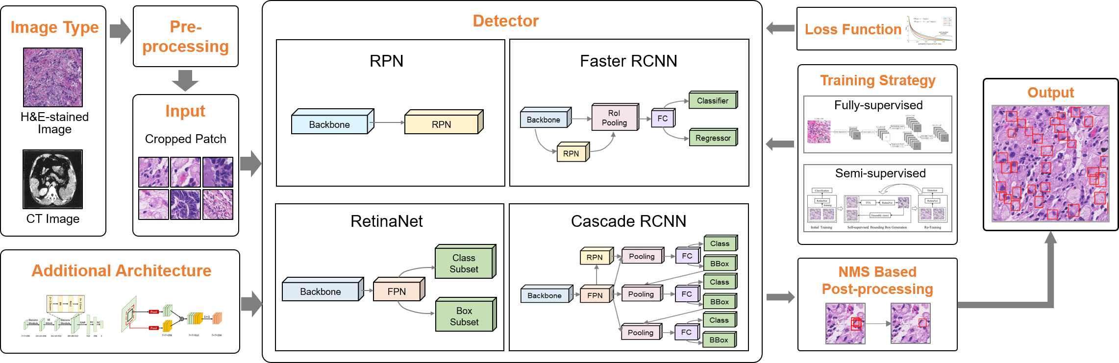
Figure 3: An overview of detection methods for SRC diagnosis.

Table 3: Summary of automatic SRC diagnosis algorithms on the basis of object detection.

Publication	Year	Modality	Target	Data	Method type	Network	Loss	SRC diagnosis
[29]	2019	CT	Peri-gastric meta-static lymph nodes	Initial group: 18,780 enhanced CT images and 1,371 labeled CT images from 313 patients Precision group: 11,340 enhanced CT images and 1,004 labeled CT images from 189 patients Verification group: 6,000 CT images from 100 patients	Two-stage, anchor based	FR-CNN(Faster-RCNN, backnone: VGG-16)	/	The differentiation level of gastric cancer consisted of well / intermediate / poor / SRC carcinoma.
[122]	2020	H&E	SRCs	Digestpath dataset	One / two-stage, anchor based	RPN, Faster RCNN, RetinaNet	CE-Loss, Smooth L1 Loss, Triplet Loss	A similarity learning approach for SRC detection.
[140]	2020	H&E	SRCs	Digestpath dataset	One / two-stage, anchor based	Cascade RCNN (backbone: ResNet-50 with FPN)	Smooth L1 Loss and CE-Loss	SRC detection with classification reinforcement detection network.
[18]	2021	H&E	SRCs	Digestpath dataset	One / two-stage, anchor based	Cascade RCNN (backbone: ResNet-50 with FPN)	Smooth L1 Loss and CE-Loss	SRC detection with classification reinforcement detection network.
[155]	2021	H&E	SRCs	DigestPath dataset for training and validation, a private dataset for test	One-stage, anchor based	USRNet, RetinaNet, Label correction model(classi-fier, backbone: ResNet-18)	RGHMC Loss	The framework provided an essential method for SRC detection in low-resolution pathological images.
[148]	2021	H&E	SRCs	DigestPath and MoNuSeg [62] dataset	One-stage, anchor based	Two RetinaNets (backbone: ResNet-18) for classification and detection respectively	Focal Loss for classification, Smooth L1 Loss for box regression	A semi-supervised deep convolutional framework for SRC detection to deal with the issue of incomplete annotations.
[76]	2021	H&E	SRCs	Digestpath dataset	One-stage, anchor based	RetinaNet (backbone: ResNet-18)	DGHM-C Loss	A novel DGHM-C Loss was proposed for partially annotated SRCs detection.
[123]	2021	H&E	Nuclei and SRCs	DigestPath and MoNuSeg dataset	One / Two-stage, anchor based	RPN, Faster RCNN, RetinaNet (backbone: ResNet-50 / ResNet-101 / ResNeXt-101)	CE-Loss and Focal Loss for classification, Smooth L1 Loss for regression, Pair Loss and Triplet Loss for embedding	A general similarity-based method for both nuclei and SRCs detection.
[112]	2022	H&E	SRCs	200 images (99 from two hospitals and the others from internet sources)	Two-stage, anchor based	Fast-RCNN (backbone: ResNet-50)	Smooth L1 Loss, CE-Loss	The SRCs were annotated by bounding boxes and detected by a general detection method.
[89]	2023	H&E	SRCs	770 patches with size from 108 WSIs of 9 patients	Two-stage, anchor based	C3Det [70], Faster-RCNN (backbone: ResNet50)	Not mentioned	An interactive detection method with bounding boxes generated by NuClick [58].
[37]	2023	H&E	SRCs	DigestPath dataset	One-stage, anchor based	RetinaNet	CE-Loss	The learned representation from multiple H&E data sources could be used to improve the performance of additional tasks via transfer learning such as SRC detection.

3.3.1 Backbone

Backbone network was one of the most important components of state-of-the-art (SOTA) detectors. Among them, VGG [115], ResNet [41] and ResNeXt [144] were three typical backbone architectures utilized for SRC detection.

VGG. VGG was proposed on the basis of AlexNet. Differently, VGG used small convolution kernels to increase the network depth. VGG achieved advanced results on ImageNet and became one of the most commonly used backbone networks for image classification and object detection. For SRC detection, VGG16 was a popular choice as the backbone network.

ResNet. ResNet with residual blocks was proposed to alleviate degradation risks. ResNet won the first place in all five main tracks of ILSVRC 2015 and MS COCO 2015 competitions, and achieved robust and good performance in many specific tasks. For SRC detection, the ResNet-18, ResNet-50 and ResNet-101 architectures were commonly adopted as the backbone networks.

ResNeXt. ResNeXt was proposed based on ResNet and Inception module [125], which adopted group convolution modules in residual blocks, namely, the “split-transform-merge” mode of Inception. Additionally, a simple and efficient architecture was achieved by applying identical topological paths in ResNeXt blocks instead of the elaborate Inception transformation. Cardinality was the only hyperparameter to control the number of convolutional paths, which could be considered as the third dimension of the data to improve the performance in addition to width and depth. Therefore, ResNeXt could achieve higher accuracy while consuming slightly fewer parameters than a similar depth ResNet architecture. ResNeXt won the runner-up of the ILSVRC 2016 challenge . The typical ResNeXt-50 and ResNeXt-101 have been applied to the SRC detection.

3.3.2 Detector

Detector, namely, the entire object detection network, output the classification and localization results of objects. According to whether and how many region proposal modules were introduced, there were three types of detectors: one-stage (e.g., RetinaNet [78]), two-stage (e.g., Faster RCNN [109]) and multi-stage (e.g., Cascade RCNN [11]) detectors. Among them, four frequently used detectors for SRC detection shown in Fig. 4 are presented in this section.

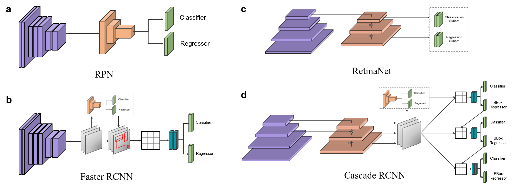
Figure 4: The typical architectures of detectors for SRC detection. (a) RPN [109]. (b) Faster RCNN [109]. (c) RetinaNet [78]. (d) Cascade RCNN [11].

Region proposal network (RPN). Region proposal methods and region-based CNNs (RCNNs) were two essential components of the two-stage detectors. Nevertheless, traditional region proposal methods such as Selective Search [135] and EdgeBoxes [163] were time-consuming, making it impossible for the detectors to be real-time. The introduction of RPN [109] (Fig. 4a) made the process almost cost-free. It took the feature maps from the backbones of an arbitrary image as input and output bounding boxes and corresponding scores of objects. Particularly, anchor boxes were introduced as localization references with various sizes and aspect ratios. Specifically, RPN slided over the feature maps extracted from backbones with a 3$\times$3 convolutional kernel and obtained a 256-dimension feature vector for each location. These feature maps were then fed into two branches: one for classification and another one for regression. The branch for classification generated the confidence probability for each predicted box containing corresponding object, and the branch for regression refined the position and size of each bounding box based on the corresponding anchor. RPN was widely used in current two-stage detection networks, such as Faster RCNN and Cascade RCNN. For SRC detection, it was also served as an independent detection network.

Faster RCNN. Faster RCNN (Fig. 4b) was one of the most popular two-stage detectors. It was essentially a Fast RCNN [30] with RPN which was the core novelty as a nearly cost-free proposal algorithm. The backbone network served images as input and generated feature maps which were then fed into RPN to obtain region proposals. Next, the chosen proposals were mapped back to the previous feature maps in RoI Pooling layer and fed into fully connected layers to obtain ultimate classification and regression results. The training process of Faster RCNN contained four steps. First, the backbone network was initialized with the parameters pretrained on the ImageNet dataset and the RPN was fine-tuned end-to-end. Second, Fast RCNN was trained with another pretrained model and rectangular proposals generated by the RPN of last step. Then, only the parameters of RPN were updated while the rest parameters of the model in the second step were fixed. Finally, the parameters of the RPN and the backbone were fixed, and the unique layers of Fast RCNN were fine-tuned. Faster RCNN was the first unified and near real-time object detection framework based on deep learning, and its core principles have inspired many subsequent detectors. In addition, Faster RCNN has also been widely used in SRC detection.

RetinaNet. One-stage detectors were popular for their high speed and simpleness, but their precision was far behind that of two-stage detectors. In two-stage detectors, sparse sampling and NMS algorithm helped filter out most negative samples in the RPN to attain better performance. To alleviate extreme imbalance between foreground and background in dense detection with one-stage detector, Lin et al. proposed a novel classification loss called Focal Loss [78] reduce the loss weights of the simple samples and focus on the hard ones. To verify the effectiveness of Focal Loss, Lin et al. also proposed a simple one-stage detector, RetinaNet (Fig. 4c), which utilized the Feature Pyramid Network (FPN) [77] to extract and fuse features of different layers from the backbone, and used two similar sub-nets at each layer for classification and regression, respectively. One the one hand, detection of multi-scale objects was implemented at different levels of feature maps. One the other hand, features with high-level semantic information and high resolution were integrated, which was beneficial for classification and localization. RetinaNet surpassed all the other detectors in both accuracy and speed when it was proposed, so it has been widely used in SRC detection.

Cascade RCNN. In the training process of RPN, an Intersection and union (IoU) threshold was defined to classify positive and negative examples. A detector tended to generate noises with a relative low threshold, while suffered a performance degradation with increasing the IoU threshold. Two main reasons for this problem were considered: one was the overfitting due to rapid reduction of positives, and another one was the mismatch of the proposal quality between training and test. Cai et al. demonstrated that regressors trained with different IoU thresholds could provide the best optimization for samples of IoU close to the corresponding thresholds [11]. To this end, a multi-stage object detection framework, Cascade RCNN (Fig. 4d) was proposed to gradually improve the quality of the bounding boxes to alleviate the problems of overfitting in the training process and quality mismatch in the inference process. Specifically, three detectors were trained in a cascaded way with IoU thresholds of 0.5, 0.6, 0.7, while each detector adopted the optimized bounding boxes from the previous stage, thereby refining the proposals step by step. As a result, sufficient positives were produced for each stage to prevent overfitting, and cascaded optimization could also vanish the mismatch. Cascade RCNN was shown to be applicable to a wide range of object detection architectures, and it also appeared in the SRC detection task.

3.3.3 Loss functions for detection

The SRC detection task aims at generating an accurate bounding box for each SRC in the input images. According to different requirements, different novel loss functions were proposed to constrain the convergence of the models. Among them, classification loss functions were used to constrain the models to generate bounding boxes around SRCs, while regression loss functions were used to calibrate the position of the bounding boxes. Classification loss, regression loss and loss functions for other special purposes used in the SRC detection methods are described in this section.

Firstly, the classification loss functions for SRC detection are illustrated as follows.

CE-Loss. CE-Loss was exactly the most popular choice for classification tasks, which was also adopted in the classification branches of the detection models. The definition of CE-Loss used in SRC detection tasks was the same as that in SRC classification tasks (Equation 3 and Equation 4). We redefined the loss function for the convenience of the following description as

$$L_{ce-d}\left(p^{(i)},c^{(i)}\right)=\left\{\begin{array}[]{cl}-\log\left(p^{(i)}\right),&c^{(i)}=1\\ -\log\left(1-p^{(i)}\right),&c^{(i)}=0\end{array}\right.,$$ (6)

where $c^{(i)}$ is the one-hot encoded label of the sample $i$, and $p^{(i)}$ represents its predicted probability of the category with $c^{(i)}=1$. The mean value of $L_{ce-d}$ of all examples in a batch was used for back propagation, thereby promoting the model to improve the classification accuracy.

Focal Loss [78]. In object detection, dense sampling led to an extreme class imbalance, that is, a vast number of easy negatives would dominate the whole loss and thus overwhelm the training. Focal Loss was proposed to reduce the contribution of easy samples, while focus on hard and misclassified ones. For notation convenience, the gradient norm $g_{i}$ was introduced to measure the difference between prediction $p^{(i)}$ and the ground-truth $c^{(i)}$ for the sample $i$:

$$g_{i}=\left\|p^{(i)}-c^{(i)}\right\|=\left\{\begin{array}[]{cl}1-p^{(i)},&c^{(i)}=1\\ p^{(i)},&c^{(i)}=0\end{array}\right..$$ (7)

Correspondingly, Focal Loss was formulated as:

$$L_{focal}=\frac{1}{N}\sum_{i=1}^{N}\alpha g_{i}^{\gamma}L_{ce-d}\left(p^{(i)},c^{(i)}\right),$$ (8)

where $\alpha$ balanced the importance between the foreground and background, $g_{i}^{\gamma}$ denoted a modulation factor of the $L_{ce-d}$ with a focusing parameter $\gamma\geq 0$. Obviously, the relative loss of well-classified examples was down weighted when $\gamma>0$, and Focal Loss degenerated into the standard CE-Loss when $\gamma=0$. Experiments by Lin et al. showed $\gamma=2$ and $\alpha=0.25$ worked best [78].

GHMC Loss [72]. Extremely hard examples were considered as outliers, whose gradient directions tended to vary from others. Thus, models usually got confused when balancing their gradients with Focal Loss. To this end, GHMC Loss was proposed to reduce the contribution of outliers besides well-classified samples. Experiments has demonstrated that samples with gradient norm close to 0 (easy samples) or 1 (difficult samples) occupied a significantly larger proportion than others. To measure the difficulty of a sample $i$, the gradient density $GD$ and the harmonizing parameter $\beta_{i}$ were defined:

$$GD\left(g_{i}\right)=\frac{1}{l_{\varepsilon}\left(g_{i}\right)}\sum_{k=1}^{N}\delta_{\varepsilon}\left(g_{k},g_{i}\right),$$ (9)

$$\beta_{i}=\frac{N}{GD\left(g_{i}\right)},$$ (10)

where $g_{i}$ and $g_{k}$ represented the gradient norm of the $i$th and $k$th sample, respectively, and $\delta_{\varepsilon}\left(g_{k},g_{i}\right)$ represented whether $g_{k}$ was in the range centered on $g_{i}$ with the valid length $l_{\varepsilon}\left(g_{i}\right)$. $l_{\varepsilon}\left(g_{i}\right)$ and $\delta_{\varepsilon}\left(g_{k},\ g_{i}\right)$ were defined as

$$\text{For }\forall\varepsilon>0,\left\{\begin{array}[]{l}\begin{aligned} l_{\varepsilon}\left(g_{i}\right)=\min&\left(g_{i}+\frac{\varepsilon}{2},1\right)\\ &-\max\left(g_{i}-\frac{\varepsilon}{2},0\right)\end{aligned}\\ \delta_{\varepsilon}\left(g_{k},g_{i}\right)=\left\{\begin{array}[]{ll}1,&\text{if }\lvert g_{k}-g_{i}\rvert\leq\frac{\varepsilon}{2}\\ 0,&\text{otherwise}\end{array}\right..\end{array}\right.$$ (11)

Thus, $GD\left(g_{i}\right)$ denoted the gradient density around $g_{i}$, and the parameter $\beta_{i}$ varied inversely with it, which down-weighted the easy samples and outliers. Then, the GHMC Loss was formulated as

$$L_{ghmc}=\frac{1}{N}\sum_{i=1}^{N}\beta_{i}L_{ce-d}\left(p^{(i)},c^{(i)}\right).$$ (12)

RGHMC Loss [155]. RGHMC Loss was a modified version of GHMC Loss, which aimed to handle the incomplete annotation problem in the DigestPath dataset. Specifically, a considerable amount of unlabeled SRCs introduced noises to the negative set during training. Therefore, the revised ground-truth $c_{r}^{(i)}$ was introduced:

$$c_{r}^{(i)}=\left\{\begin{array}[]{l}1,x\in A_{P}\cup A_{R},A_{R}\subset A_{N}^{\text{noisy }}\\ 0,x\in A_{N}\backslash A_{R}\end{array},\right.$$ (13)

where $A_{P}$ and $A_{N}$ represented sets of original positive and negative samples, respectively, and $A_{R}$ denoted a recall set from negatives considered as SRCs. The combination of the detection model and an auxiliary classifier was implemented by Zhang et al. [155] to determine each element of $A_{R}$:

$$A_{R}=\left\{x\in A_{N}\mid l(x)=1,p^{c}(x)>t_{1},p(x)>t_{2}\right\},$$ (14)

where $p^{c}\left(x\right)$ and $l\left(x\right)$ indicated the probability and label predicted by a well-trained auxiliary classifier, respectively, $p\left(x\right)$ was the classification score of the detection network, $t_{1}$ and $t_{2}$ were two tunable thresholds. The RGHMC Loss was finally defined as

$$L_{rghmc}=\frac{1}{N}\sum_{i=1}^{N}\beta_{i}L_{ce-d}\left(p^{(i)},c_{r}^{(i)}\right).$$ (15)

DGHM-C Loss [76]. DGHM-C Loss modified the original GHMC in another way to adapt to partially annotated object detection. Lin et al. [76] argued that outliers in clean data space were probably hard samples worth learning, while those in noisy data space were rather likely to be mislabeled. To this end, a novel DGHM strategy was proposed to decouple the noisy samples from the clean ones, and the $GD$ in Equation 9 was modified separately as

$$GD\left(g_{i}\right)=\left\{\begin{array}[]{l}\frac{1}{l_{\varepsilon}\left(g_{i}\right)}\left(\sum_{k=1}^{N_{c}}\delta_{\varepsilon}\left(g_{k},g_{i}\right)\right),x_{i}\in S_{c}\\ \frac{1}{l_{\varepsilon}\left(g_{i}\right)}\left(\sum_{k=1}^{N_{n}}\delta_{\varepsilon}\left(g_{k},g_{i}\right)\right),x_{i}\in S_{n}\end{array},\right.$$ (16)

where $S_{c}$ and $S_{n}$ represented the clean data space (including annotated positives and all samples of negative images) and the noisy data space (negatives in positive images), respectively, and $N_{c}$ and $N_{n}$ were the number of their anchors. Harmonizing parameter $\beta_{i}$ was also redefined with a modulating factor $\gamma_{i}$:

$$\beta_{i}=\frac{N}{GD\left(g_{i}\right)^{\gamma_{i}}},$$ (17)

$$\gamma_{i}=\left\{\begin{array}[]{ll}\mu_{n},&g_{i}\geq\lambda,x_{i}\in S_{n}\\ \mu_{c},&g_{i}\geq\lambda,x_{i}\in S_{c}\\ 1,&\text{ otherwise }\end{array},\right.$$ (18)

where $\gamma_{i}$ had two different values for outliers exceed the threshold $\lambda$ in $S_{c}$ and $S_{n}$. In general, $\mu_{n}\geq 1$ was selected to reduce the weight of outliers in $S_{n}$ to prevent overfitting to noises, and $\mu_{c}\leq 1$ was chosen at the same time to up-weight the outliers in $S_{c}$ to achieve hard sample mining. In SRC detection, $\mu_{n}=2.0$, $\mu_{c}=0.5$, and $\lambda=0.9$ were taken as default settings [76]. The whole DGHM-C Loss was finally defined as

$$L_{dghm-c}=\frac{1}{MN}\sum_{i=1}^{N}\beta_{i}L_{ce-d}\left(p^{(i)},c^{(i)}\right),$$ (19)

where $M$ was the number of gradient norm distributions.

Secondly, the regression loss functions for SRC detection are illustrated as follows.

Smooth L1 Loss [30] was applied in almost all SRC detectors. It was first proposed in Fast RCNN [30] to replace L2 Loss used in SPPNet [40] and R-CNN [31]. Smooth L1 Loss alleviated sensitivity to outliers, so as to prevent gradient explosion in training. A four-dimensional vector $\vec{b}=<x,y,h,w>$ was required to be regressed for each predicted bounding box, where $x$ and $y$ were the normalized coordinates of the center of the bounding box, $h$ and $w$ represented the height and width of the bounding box, respectively. Similarly, $\vec{b_{a}}=<x_{a},y_{a},h_{a},w_{a}>$ and $\vec{b^{\ast}}={<x}^{\ast},{\ y}^{\ast},\ h^{\ast},\ w^{\ast}>$ were introduced to encode an anchor box and the ground truth, respectively. Regression offsets could be calculated as follows:

$$\left\{\begin{array}[]{ll}t_{x}=\left(x-x_{a}\right)/w_{a},&t_{x}^{*}=\left(x^{*}-x_{a}\right)/w_{a}\\ t_{y}=\left(y-y_{a}\right)/h_{a},&t_{y}^{*}=\left(y^{*}-y_{a}\right)/w_{a}\\ t_{h}=\log\left(h/h_{a}\right),&t_{h}^{*}=\log\left(h^{*}/h_{a}\right)\\ t_{w}=\log\left(w/w_{a}\right),&t_{w}^{*}=\log\left(w^{*}/w_{a}\right)\end{array}\right.,$$ (20)

where $<t_{x},t_{y},t_{h},t_{w}>$ denoted the offsets between the prediction and the anchor box, and $<t_{x}^{\ast},t_{y}^{\ast},t_{h}^{\ast},t_{w}^{\ast}>$ denoted the offsets between the anchor box and the ground truth. Then, the Smooth L1 Loss was calculated as

$$L_{\text{smoothL}_{1}}\left(\vec{t},\vec{t}^{*}\right)=\sum_{j\in\{x,y,h,w\}}f\left(t_{j}-t_{j}^{*}\right),$$ (21)

where $\vec{t}=<t_{x},t_{y},t_{h},t_{w}>$, and ${\vec{t}}^{\ast}=<t_{x}^{\ast},t_{y}^{\ast},t_{h}^{\ast},t_{w}^{\ast}>$, $f(\cdot)$ was defined as

$$f(x)=\left\{\begin{array}[]{cl}0.5x^{2},&\text{ if }\lvert x\rvert<1\\ \lvert x\rvert-0.5,&\text{ otherwise }\end{array}\right.$$ (22)

Thirdly, other loss functions for SRC detection are illustrated as follows.

Auxiliary embedding layers were also introduced in some SRC detection methods to learn discriminative features, such as similarity learning embeddings [122, 123] with pair loss [38] or triplet loss [43]. We will introduce these two loss functions in this section.

Pair Loss [38]. In the task of SRC detection, Sun et al. use the Pair Loss to pull the anchors of the same category closer, while pulling away the anchors of different categories in the embedding space [123]. Pair Loss was defined as

$$\begin{array}[]{rl}L_{\text{pair}}\left(\sigma,\sigma^{\prime},s\right)=&s\left\|\sigma-\sigma^{\prime}\right\|^{2}/2+(1-s)\\ &\max\left(m-\left\|\sigma-\sigma^{\prime}\right\|^{2},0\right)/2,\end{array}$$ (23)

where $\sigma$ and $\sigma^{\prime}$ represented the embeddings of two sampled anchors, $s\in\left\{0,1\right\}$ denoted the closeness between them, $\left\|\cdot\right\|$ was the Euclidean distance metric, and $m$ was a constant of margin. It could be observed that as the loss function decreased, the distance between two samples of different categories should be greater than $m$, while samples of the same class were getting closer. It enabled the models to learn more discriminative features, which benefited the subsequent classification.

Triplet Loss [43]. Triplet Loss was another popular loss function for similarity learning. Its purpose was similar to Pair Loss (Equation 23) with a different form calculated among three samples:

$$\begin{array}[]{r}L_{\text{triplet}}\left(\sigma^{a},\sigma^{p},\sigma^{n}\right)=\max(\left\|\sigma^{a}-\sigma^{p}\right\|^{2}\\ -\left\|\sigma^{a}-\sigma^{n}\right\|^{2}+m,0),\end{array}$$ (24)

where $\sigma^{a}$ was a reference embedding, and $\sigma^{p}$ was a positive embedding of the same category with the reference while $\sigma^{n}$ represented a negative one of another category. After optimization, the distance between $\sigma^{a}$ and $\sigma^{p}$ would be less than that between $\sigma^{a}$ and $\sigma^{n}$ by a margin of $m$.

3.3.4 Training strategy

Fully supervised learning. Fully supervised learning was the most common training strategy in SRC detection [29, 155, 76, 122, 140, 18, 123, 112]. Models could achieve satisfactory performance with sufficient training data and high-quality annotations. However, DigestPath dataset suffered from a problem of incomplete labeling, which introduced noises during training stage. Besides, variation in color, shape, size, scale, and the overlaps of SRCs also brought great challenges to detection. Most of the existing studies implemented the SRC detection by fully supervised learning which relied entirely on accurate annotations of the training data. These solutions could be divided into two categories: methods based on modified loss functions and auxiliary modules. Among them, the loss functions were refined to make the models more robust. For example, Zhang et al. proposed the RGHMC Loss (Equation 15) with a label correction module which treated the revised ground-truth labels as the reference for calculating gradients [155]. Lin et al. decoupled noisy samples from clean ones and devised the DGHM-C Loss (Equation 19) to harmonize their gradient distributions respectively [76]. In addition, some methods employed additional auxiliary modules to enable the model to learn discriminative features for enhancing the classification. For example, Wang et al. and Chen et al. designed a Classification Reinforcement Branch (CRB) to extract more comprehensive features containing cells and their surrounding context [140, 18]. Sun et al. introduced an embedding layer to perform similarity learning, which adopted Pair Loss (Equation 23) or Triplet Loss (Equation 24) to narrow the intra-class distance and expand the inter-class one [122, 123].

Semi-supervised learning. Semi-supervised learning aimed to handle the issue of lack of well-labeled data. However, among the current SRC detection methods, only Ying et al. applied the semi-supervised learning strategy [148]. Specifically, a simple but efficient self-training framework was proposed to deal with the partial annotations in DigestPath dataset, which could be divided into three procedures. In the first step, an initial RetinaNet [78] model was trained with annotated labels. During the inference time, the pseudo bounding boxes were generated by the initial network, and then filtered by the novel Test Time Augmentation (TTA) and modified NMS algorithms to supplement the dataset with high-quality labels. With the new dataset, an iteratively retraining could be performed until there was no improvement of the detector. They achieved the 1st place in the SRC detection task of the Digestive-System Pathological Detection and Segmentation Challenge 2019, which demonstrated a superior potential of semi-supervised learning in this task.

3.4 Segmentation

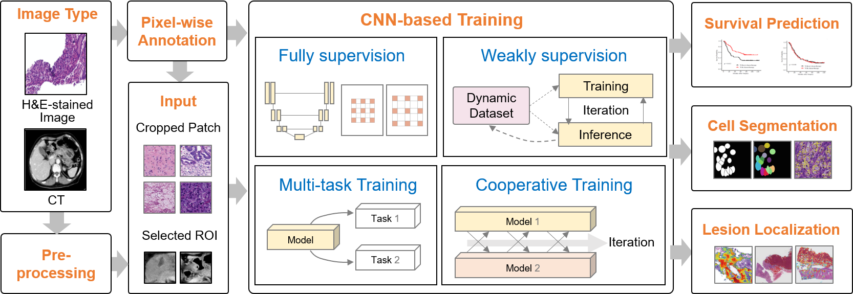
Figure 5: An overview of segmentation methods for SRC diagnosis.

Segmentation clearly outlined the shape of the lesions. Unlike classification algorithms that mapped an input patch to a single category, segmentation algorithms mapped a patch to a diagnostic heatmap with the same size as the input patch. Therefore, segmentation algorithms could perform delicate and complex tasks such as cell segmentation. As shown in Fig. 5, among the articles related to SRC diagnosis covered in this survey, the segmentation algorithms completed four training strategies, namely, full supervision, weak supervision, multi-task training, and cooperative training, to complete sub-tasks such as survival prediction, cell segmentation, and lesion localization. The overview of articles related to SRC segmentation is summarized in Table LABEL:table:Seg. The details of CNN-based training strategies and task-related post-processing are presented next.

Table 4: Summary of automatic SRC diagnosis algorithms on the basis of segmentation.

Publication	Year	Modality	Target	Task	Data	Network	Loss	SRC diagnosis
[73]	2022	CT	SRC carcinoma	SRC carcinoma diagnosis and chemotherapy response prediction	855 images (the maximum cross sections of precontrast for each patient)	U-Net	CE-Loss	Segmentation encoder was assigned on only one single slice of a 3D matrix for each patient to diagnose SRC carcinoma.
[74]	2019	H&E	SRC	SRC segmentation with a semi-supervised learning framework	127 WSIs from 10 organs (at least 3 cropped regions for each WSI)	U-Net with ResNet-34 or DLA as the encoder	CE-Loss, IOU-Loss	Multi-organ SRC segmentation with relatively small amount of annotation cost.
[119]	2020	H&E	Gastric cancer	A two-class system to distinguish between benign and malignant	6917 WSIs from 3 centers	DeepLab-v3 with ResNet-50 as the backbone	CE-Loss	SRC carcinoma was included in the malignant category and was easily overlooked when there were limited cancer cells.
[151]	2021	H&E	Gastric cancer	Screening and localization of gastric cancer based on a multi-task CNN	10,315 WSIs collected from 4 medical centers	DLA structure combined with classification and segmentation branches	BCE-Loss	SRC carcinoma was one type of the positive targets.
[6]	2022	H&E	Gastric cancer	Assessment of deep learning assistance for the pathological diagnosis	110 WSIs and 16 board-certified pathologists	DeepLab-v3 with ResNet-50 as the backbone	CE-Loss	SRC carcinoma was included in the malignant category and deep learning could help pathologists improve the diagnosis accuracy of scattered SRCs.
[21]	2022	H&E	Gastric SRC carcinoma	Quantifying the cell morphology and predicting biological behavior	607 WSIs from stomach or colorectum	A coarse U-Net to find approximate region at $10\times$ magnification, a fine U-Net to segment SRC at $40\times$ magnification	CE-Loss, IOU-Loss	SRC segmentation was adopted to quantify the cell morphological characteristics and atypia so as to analyze the biological behavior of SRC carcinoma.
[130]	2022	H&E	Lung Cancer	Prediction of ALK gene rearrangement in patients with non-small-cell lung cancer	300 WSIs from 208 patients	DenseNet-121 with up-sampling and skip connections	BCE-Loss	SRC carcinoma was considered in the histologic types of surgical specimen.
[1]	2022	H&E	Gastric cancer	Development and multi-institutional validation of an AI-based diagnostic system for gastric biopsy	984 patients for training and 2771 patients for validation	U-Net	Not mentioned	The performance of a poorly cohesive adenocarcinoma with SRCs was discussed.
[55]	2023	H&E	Colorectal cancer	Lymph node segmentation and metastasis detection	100 WSIs of lymph node regions from 14 patients for segmentation	U-Net	BCE-Loss, CE-Loss	In a validation cohort with mucinous and SRC histology, the performance was slightly worse because of limited examples.
[158]	2023	H&E	Colorectal cancer	Hybrid deep learning framework for tumor segmentation	DigestPath and GlaS [116] datasets	RGSB-UNet derived from U-Net, residual block, and bottleneck Transformer	Class-wise Dice Loss	SRC carcinoma was regarded as one type of malignant lesions in this study.

3.4.1 CNN-based training strategies

Fully supervised training. Segmentation put forward high requirements with accurate pixel-wise annotation. The fully supervised trained segmentation algorithms could both capture SRC-positive regions in CT images [73] and localize lesion regions in H&E stained images [74, 119, 55, 158]. U-Net [110], DeepLab [13] or their variants were usually used as the skeleton networks. U-Net was a U-shaped network with encoder-decoder structure originated from the task of cell segmentation. The encoder extracted high-level semantic information through continuous down-sampling, the decoder restored the image size by up-sampling, and the encoder transmitted spatial location information to the decoder through skip-connections. DeepLab used VGG, ResNet and other classic classification network structures as the basic backbone, expanded the receptive fields through atrous convolution, and finally improved the segmentation performance through conditional random field (CRF) [64]. Then its variant DeepLab v3+ [14] removed the time-consuming CRF, and further improved the integration ability of spatial information through Atrous Spatial Pyramid Pooling (ASPP) [151]. Segmentation algorithms often used CE-Loss (Equation 3) to constrain pixel-wise prediction. In addition, intersection over union loss (IOU-Loss) [152] and Dice-Loss [95] were popular for the positive region prediction. IOU-Loss $L_{iou}$ and Dice-Loss $L_{dice}$ were defined as

$$L_{iou}=1-\frac{\sum_{i}{y_{i}p_{i}}}{\sum_{i}y_{i}+\sum_{i}{p_{i}-\sum_{i}{y_{i}p_{i}}}},$$ (25)

$$L_{dice}=1-\frac{2\sum_{i}{y_{i}p_{i}}}{\sum_{i}y_{i}^{2}+\sum_{i}p_{i}^{2}},$$ (26)

where $y_{i}$ and $p_{i}$ were the ground truth and predicted probability for the pixel $i$, respectively.

Multi-task Training. Classification was the global control of the input image patch, while segmentation was the local control of the details of that. Since classification and segmentation had complementary advantages, multi-task training could constrain model optimization from both global and local levels. For example, Yu et al. embedded two parallel branches after feature extraction in the backbone network to achieve classification and segmentation simultaneously [151]. Multi-task learning could balance different requirements simultaneously.

Weakly supervised training. Although fully supervised segmentation algorithms could handle many segmentation requirements, there were often situations in which data annotations mismatched the task objectives in reality. For example, DigestPath dataset annotated SRCs with rectangular boxes that contained SRCs without outlining their contours. Therefore, Li et al. achieved SRC segmentation by weakly supervised learning [74]. They approximated the contours of SRCs by generating inscribed ellipses within the bounding boxes. Although this operation inevitably led to labeling errors, the ellipses could be used as training data for the fully supervised segmentation methods described above. Given that there were a large number of unlabeled SRCs in the slides, the early-stage segmentation model was adopted to segment the unlabeled data, and some positive regions with the highest confidence probabilities were added to the training set for retraining. The training and inference alternated to achieve self-training, and then gradually improved the model accuracy.

Cooperative training. Different network structures often had different emphasis on feature extraction. Therefore, some algorithms fused the inference output of different models to improve the final diagnostic performance. For example, Li et al. replaced the encoder of U-Net with ResNet and DLA [150], respectively, resulting in two different networks [74]. Then, the self-training strategy mentioned above was adopted for the two networks. In the iterative process, the inference results of the other network were used to strengthen the training, so as to realize the information exchange of different networks. The two models converged to be consistent in performance while improving accuracy. Such a cooperative training strategy could avoid a single model from getting stuck in local optima.

3.4.2 Task-related post-processing

Survival prediction. The segmentation algorithms directly presented the SRC positive regions, which was very convenient for the evaluation of SRC aggregation degree, lesion area and other metrics. Therefore, segmentation played an important auxiliary role in the formulation of clinical diagnosis and treatment strategies. For example, Li et al. extracted SRC carcinoma features through segmentation models to identify patients who could benefit from postoperative chemotherapy based on preoperative contrast-enhanced CT [73].

Cell segmentation. SRCs could either aggregate in clusters or distribute in isolation. Segmentation methods that took the lesion area as a whole tend to miss isolated SRCs. In addition, when suggesting the existence of SRCs, providing quantitative information such as the degree of cell aggregation was more interpretable and convincing clinically. Therefore, cell segmentation for SRCs was an efficient and intuitive basis for quantitative analysis. The challenge of cell segmentation was that cell-level annotation was time-consuming and labor-intensive. Li et al. utilized weakly supervised learning and cooperative training to train a cell segmentation model on the basis of bounding box annotations [74]. Then, Da et al. adopted the segmented results to measure the inherent properties of SRCs including the cross-sectional area of cell plasma and nuclear, the cell ellipticity, as well as the nuclear / cytoplasmic ratio [21].

Lesion segmentation. Similar to lesion classification, lesion segmentation combined patch-level results into a diagnostic heatmap corresponding to the slide by splicing. The difference was that the segmentation was a pixel-wise classification, that is, the size of the diagnostic heatmap was the same as the original slide. Due to the mining of details by the segmentation algorithms, it was possible to focus on small lesions. Song et al. developed a gastric cancer lesion segmentation system based on DeepLab v3+ [119]. Ba et al. further demonstrated that the system assistance indeed improved pathologists’ accuracy in gastric cancer diagnosis [6]. However, the components in H&E stained slides were complex. Many factors led to the inevitable false positive noise or false negative holes in pixel-by-pixel analysis. Therefore, Yu et al. embedded both classification and segmentation branches in the backbone network. The classification branch was used to control global features, and the segmentation branch was used to refine local features, so as to obtain diagnostic heatmap results that were more in line with the actual diagnosis experience of pathologists [151].

4 Discussion and future outlook

4.1 SRC datasets for learning

The fitting of models based on deep learning was driven by big data, which put forward high requirements for the quantity and quality of data. There were a few studies on SRC automatic diagnosis in CT, MRI, and endoscopy images, and they were conducted on private datasets [73, 29, 82, 149, 147, 33]. More studies focused on accurate identification of SRCs in histopathological images, including the public datasets TCGA and DigestPath, and some private datasets. Specifically, in the task of gastrointestinal tract malignancy discrimination, although the number of patients in the datasets was large due to high morbidity, SRC carcinoma was only a special type of positive samples with few cases [103, 60, 45, 48, 71, 151, 20, 119]. The imbalance of samples in the training set often led to the inevitable omission of valuable SRCs in inference [103, 60, 45, 20, 119]. In addition, the training set of the DigestPath dataset dedicated to SRC detection was composed of images from only 20 positive WSIs. Compared with natural images, the data scale of SRCs was very limited. For example, the emergence of ImageNet [23], a dataset with one million natural images, promoted the birth of excellent classification networks such as AlexNet, ResNet, VGG, and GoogLeNet. Recently, self-supervised learning has attracted much attention. Among them, the typical algorithm MoCo [39] captured the effective features of images through pretext tasks in Instagram-1B [93], a dataset containing about one billion images. However, the privacy of medical data and the time-consuming of accurate labeling inevitably limited the size of the SRC datasets, and thus inhibiting the performance promotion of fully supervised learning [106]. To increase the robustness of the models as much as possible, when classical networks such as VGG and Inception were used to automatically diagnose SRCs, the parameters pretrained on the natural image datasets were often loaded before training to avoid the model overfitting or falling into local optimal solutions. In addition, to increase the generalization of the models, data augmentation was often embedded in the pre-processing process. Common data augmentation methods used in SRC pre-processing included random flipping, rotation, and color fluctuation. Although GAN [32] and its variants could normalize image styles and synthesize more images, it introduced a lot of additional time consumption and data trust crisis [106, 63]. These methods improved the accuracy of the models from the perspective of technology, but they did not increase the number of real cases in essence.

In the future, the size of the datasets will not be limited to absolute numbers, but focus on the size of effective high-quality data. Current data augmentation methods did not enable the models to see diverse real-world cases, and the generalization performance remained limited during inference. Therefore, new and clinically challenging datasets should be constructed, in which the following four points may be paid special attention.

• To evaluate the generalization and robustness of the models in practical applications, the data are required to be derived from different medical centers and cover multiple scenes such as biopsy and surgical specimens.

• Since SRCs are lesions that can develop in various tissues and organs, the cases in the datasets should break through the common limitations of the gastrointestinal tract, and clearly indicate the primary and metastases.

• Typical SRC distributions may be involved, including aggregated and isolated cases.

• Multi-modal data are expected to be matched, such as age, gender, genes, and survival time, to facilitate further clinical studies.

4.2 Selection of training strategy

Fully supervised learning was considered robust and effective in natural image processing with sufficient training data. Despite the relatively limited amount of data in medical images compared to natural images, the models could still capture the typical morphological and structural features in the training data. When the input images had explicit expert annotations, fully supervised learning allowed the models to quickly obtain preliminary automatic diagnostic performance. The performance of the model was closely related to the data distributions of the training set. When the typical SRCs were few in the training set, the models would inevitably be biased towards other categories with more patients to obtain high accuracy in the evaluation [60, 50]. Therefore, when SRCs were mixed in the data of multiple subtypes of the gastrointestinal tract, special attention was needed to be paid to the problem of class imbalance, thereby improving the sensitivity of SRCs. However, fully supervised learning strongly relied on the fine-grained annotations, which required the pathologists to specify the location of each SRC. The time-consuming and laborious labeling requirements led to the scarcity of labeled data, which limited the scale of training data for fully supervised learning.

SRCs were difficult to be completely outlined even by experienced pathologists, so completely accurate fine annotations were almost impossible within limited time and cost. To ensure the accuracy of the annotations, some typical SRCs were carefully selected to teach the model learning and the confusing ones were ignored. Incomplete labeling was a ubiquitous phenomenon in SRC detection tasks [22]. In addition to fully supervised learning with only limited annotations, semi-supervised learning further considered unlabeled SRCs [148]. Incomplete labeling ensured the purity of the positive sample set, but could not guarantee the purity of the negative sample set, so it introduced a lot of noise to the learning of negative samples. Semi-supervised learning is an effective approach to reduce annotation pressure in the future, but the following two open issues need to be solved. First, how to obtain the high-dimensional representation of typical SRC features with only a few samples? Second, how to extract unlabeled true positive samples and eliminate false positive samples?

Weakly supervised learning can alleviate the dilemma of the scarcity of effective training data for fully supervised learning. Patient-level labels can be obtained directly from the current diagnosis pipeline. When a patient is diagnosed with SRCs, the corresponding screening images must contain SRCs although the specific location of each SRC is not specified. Weakly supervised learning embeds data with patient-level labels or image-level labels into the training set, greatly reducing the labeling pressure of pathologists and increasing the size of the training set. Combining fully and weakly supervised learning can balance the contradiction between SRC labeling pressure and training set size [52, 20]. In the future, weakly supervised algorithms should be mined deeply to make use of the SRC data containing patient-level labels already stored in various medical centers. In addition, additional SRC data collected over time may also be utilized to improve model performance without additional annotations.

Unsupervised learning is a valuable but also challenging training strategy for future research. A large amount of data without manual annotations can be utilized by unsupervised learning to actively cluster similar samples. In the early stage, the self-supervised learning strategy can train encoders through pretext tasks such as out-of-order correction and cloze [39]. The encoders with pretrained parameters are then fine-tuned on specific tasks, obtaining encoders that can extract SRC generalization features and well-performing decoders. In the later stage, ideal unsupervised learning will adaptively aggregate homogeneous tissues in the images into fine-grained subcategories, such as SRC nuclei, intracellular proteins, normal nuclei, and lymphocytes. Then, they are combined into target categories according to requirements, such as SRCs and lesion regions containing SRCs.

4.3 From algorithms to assistance

The algorithms designed for the DigestPath dataset detected typical SRCs in gastrointestinal histopathological patches [22, 148], but were not suitable for clinically complex screening of SRCs in multiple organs. Most algorithms only accomplished SRC diagnosis for specific datasets, which ignored the attribute information such as the originated organs and invasion degrees, thus hindering subsequent prognosis. To complete the transition from algorithms to diagnostic assistance, future studies need to make contributions in the following four aspects.

• Following the pathologists’ pipeline of diagnosing lesions from different fields of view by changing the magnification of the microscope, the intelligent algorithms may consider the multi-scale features. Kosaraju et al. distributed the detection of gastric lesions at 20$\times$ and 5$\times$ magnifications through two different branches [60]. To simulate the visual diagnostic habits of the human eyes, more scales should be considered in future algorithms. Clustered SRCs can be detected at a faster speed at low magnification, while isolated SRCs will not be missed at high magnification.

• Special attention could be provided to SRCs of metastases. Although SRCs occur mostly in the gastrointestinal tract, they may appear in various organs such as lung, pancreas, appendix, gallbladder, breast, and bladder [7]. For example, metastatic SRCs may stimulate tissue proliferation in the ovary, making SRCs more difficult to identify. When SRCs are implanted in the body cavity, omentum peritoneum, chest wall or abdominal wall of the patients, the surgical procedure and systemic treatment strategy will be affected.

• The prognosis of SRCs will be directly correlated by algorithm-based lesion quantification. Prognosis through high-dimensional representation of SRCs in CT and MRI has been initially practiced and the feasibility was demonstrated [73, 82]. Since histopathology plays an important role in the diagnosis of SRCs, there is great research values and improvement room to realize prognosis prediction based on intelligent features. In addition, prognostic factors such as sampling location and depth of invasion may also be embedded in the intelligent analysis process in the future.

• Future algorithms should be oriented to assistant needs throughout the entire diagnosis process. The current algorithms usually only solved a single problem in a simple scenario, such as SRC identification in gastric pathological slides. In the future, an end-to-end AI framework that fits the clinical diagnosis process will be welcomed, thereby promoting the implementation from algorithms to assistance.

4.4 Multi-modal diagnosis

This survey exclusively addresses algorithms that leveraged deep learning to automatically extract features from medical images. It omits the methods solely inferring prognosis directly from clinical information such as age, gender, and tumor characteristics, as these approaches still depended on manual interpretation [75, 65, 131, 161, 157, 159, 17, 156]. Meanwhile, methods involving manual delineation of RoIs in CT images for subsequent local feature extraction and fusion with clinical information for prognosis analysis were also excluded [153, 16, 80]. Notably, both image-based and clinical information-based algorithms started from a single modality, disregarding the diagnostic potential of other modalities, which does not align with actual clinical diagnostic workflows. Therefore, future AI algorithms should balance the multi-modal predicted results to improve the diagnostic accuracy. The great potential of multi-modal learning for cancer prognosis analysis has been demonstrated by a study using multi-modal learning to integrate and analyze WSIs and genetic maps of 14 cancers [15]. Furthermore, machine learning approaches integrating lipidomics and multi-omics have been demonstrated to be beneficial for the detection of lung cancer and pancreatic ductal adenocarcinoma [138, 139]. Additionally, radiographs, unstructured chief complaint and clinical history, and structured clinical information such as laboratory test results and patient demographic information were converted into visual tokens and text tokens to accomplish a Transformer-based representation model to help streamline the triaging of patients [162]. Therefore, the joint analysis of multi-modal information such as CT, histopathology, genomics, and lipidomics based on AI algorithms is the development trend of SRC precise localization, exploration of new detection methods, and accurate prognosis in the future.

5 Conclusions

In this survey, we have presented a comprehensive overview on automatic SRC diagnosis developed by AI-related algorithms. With the popularity of deep learning in the field of intelligent medicine, automatic algorithms for SRCs that were at risk of missed detection even for experienced pathologists have emerged. Since the lack of a comprehensive survey prevented researchers from intuitively accessing the development of SRC intelligent algorithms and the gap towards clinical applications, we collated articles with automatic algorithms for SRC diagnosis to form this survey. Specifically, this survey covered articles from 2008 to August 2023, involving H&E stained histopathology WSIs, CT, MRI and endoscopic images. First, we refined the current challenges of automatic SRC diagnosis. Then, currently available public datasets were introduced. After the general pre-processing methods were illustrated, the algorithms were summarized into three categories, i.e., classification, detection, and segmentation. To clarify the post-processing details of the specific applications, above methods were further decomposed into sub-tasks according to application scenarios, such as lesions classification, cell detection, cell segmentation, lesion segmentation, and survival prediction. Finally, we discussed the limitations of current algorithms facing clinical applications and provided future research trends in SRC dataset construction, available training strategies, assistance pipelines, and multi-modal diagnosis. In summary, the methods and datasets categorized and summarized in this survey can be regarded as a guide for the technological exploration of SRC automatic diagnosis. Researchers in related fields, especially who without medical background can intuitively obtain the clinical requirements for intelligent assistance and potential research directions in the future. In addition, this survey provides a feasible reference for intelligent diagnosis of other specific diseases in many aspects, including the design of assisted pipelines, algorithm optimization, and future research trends towards clinical applications.

CRediT authorship contribution statement

Zhu Meng: Conceptualization, Investigation, Formal analysis, Visualization, Funding acquisition, Writing - original draft, Writing - review & editing. Junhao Dong: Conceptualization, Investigation, Formal analysis, Visualization, Writing - original draft, Writing - review & editing. Limei Guo: Conceptualization, Investigation, Formal analysis, Supervision, Writing - review & editing. Fei Su: Conceptualization, Supervision, Writing - review & editing. Guangxi Wang: Conceptualization, Investigation, Funding acquisition, Writing - review & editing. Zhicheng Zhao: Conceptualization, Supervision, Funding acquisition, Writing - review & editing.

Declaration of competing interest

The authors declare that they have no known competing financial interests or personal relationships that could have appeared to influence the work reported in this paper.

References

- Abe et al. [2022] Abe, H., Kurose, Y., Takahama, S., Kume, A., Nishida, S., Fukasawa, M., Yasunaga, Y., Ushiku, T., Ninomiya, Y., Yoshizawa, A., et al., 2022. Development and multi-institutional validation of an artificial intelligence-based diagnostic system for gastric biopsy. Cancer Science 113, 3608–3617.
- Achanta et al. [2012] Achanta, R., Shaji, A., Smith, K., et al., 2012. Slic superpixels compared to state-of-the-art superpixel methods. IEEE Transactions on Pattern Analysis and Machine Intelligence 34, 2274–2282.
- Ahmedt-Aristizabal et al. [2021] Ahmedt-Aristizabal, D., Armin, M.A., Denman, S., et al., 2021. A survey on graph-based deep learning for computational histopathology. Computerized Medical Imaging and Graphics , 102027.
- Alsubaie et al. [2018] Alsubaie, N., Shaban, M., Snead, D., et al., 2018. A multi-resolution deep learning framework for lung adenocarcinoma growth pattern classification, in: Annual Conference on Medical Image Understanding and Analysis, pp. 3–11.
- Altini et al. [2022] Altini, N., Prencipe, B., Cascarano, G.D., et al., 2022. Liver, kidney and spleen segmentation from ct scans and mri with deep learning: A survey. Neurocomputing 490, 30–53.
- Ba et al. [2022] Ba, W., Wang, S., Shang, M., et al., 2022. Assessment of deep learning assistance for the pathological diagnosis of gastric cancer. Modern Pathology , 1–7.
- Benesch and Mathieson [2020] Benesch, M.G., Mathieson, A., 2020. Epidemiology of signet ring cell adenocarcinomas. Cancers 12, 1544.
- Bhojanapalli et al. [2021] Bhojanapalli, S., Chakrabarti, A., Glasner, D., et al., 2021. Understanding robustness of transformers for image classification, in: Proceedings of the IEEE/CVF International Conference on Computer Vision, pp. 10231–10241.
- Bosman et al. [2010] Bosman, F.T., Carneiro, F., Hruban, R.H., Theise, N.D., et al., 2010. WHO classification of tumours of the digestive system. Ed. 4, World Health Organization.
- Budak and Mençik [2022] Budak, C., Mençik, V., 2022. Detection of ring cell cancer in histopathological images with region of interest determined by slic superpixels method. Neural Computing and Applications , 1–14.
- Cai and Vasconcelos [2018] Cai, Z., Vasconcelos, N., 2018. Cascade r-cnn: Delving into high quality object detection, in: Proceedings of the IEEE Conference on Computer Vision and Pattern Recognition, pp. 6154–6162.
- Chen et al. [2021a] Chen, C.L., Chen, C.C., Yu, W.H., et al., 2021a. An annotation-free whole-slide training approach to pathological classification of lung cancer types using deep learning. Nature Communications 12, 1–13.
- Chen et al. [2014] Chen, L.C., Papandreou, G., Kokkinos, I., et al., 2014. Semantic image segmentation with deep convolutional nets and fully connected crfs. ArXiv preprint arXiv:1412.7062 .
- Chen et al. [2018] Chen, L.C., Zhu, Y., Papandreou, G., Schroff, F., Adam, H., 2018. Encoder-decoder with atrous separable convolution for semantic image segmentation, in: Proceedings of the European conference on computer vision (ECCV), pp. 801–818.
- Chen et al. [2022a] Chen, R.J., Lu, M.Y., Williamson, D.F., et al., 2022a. Pan-cancer integrative histology-genomic analysis via multimodal deep learning. Cancer Cell 40, 865–878.
- Chen et al. [2022b] Chen, T., Wu, J., Cui, C., He, Q., Li, X., Liang, W., Liu, X., Liu, T., Zhou, X., Zhang, X., et al., 2022b. Ct-based radiomics nomograms for preoperative prediction of diffuse-type and signet ring cell gastric cancer: a multicenter development and validation cohort. Journal of Translational Medicine 20, 1–13.
- Chen et al. [2023] Chen, Y., Shou, L., Xia, Y., Deng, Y., Li, Q., Huang, Z., Li, Y., Li, Y., Cai, W., Wang, Y., et al., 2023. Artificial intelligence annotated clinical-pathologic risk model to predict outcomes of advanced gastric cancer. Frontiers in Oncology 13, 1099360.
- Chen et al. [2021b] Chen, Z., Wang, S., Jia, C., et al., 2021b. Crdet: Improving signet ring cell detection by reinforcing the classification branch. Journal of Computational Biology 28, 732–743.
- Chollet [2017] Chollet, F., 2017. Xception: Deep learning with depthwise separable convolutions, in: Proceedings of the IEEE Conference on Computer Vision and Pattern Recognition, pp. 1251–1258.
- Chuang et al. [2021] Chuang, W.Y., Chen, C.C., Yu, W.H., et al., 2021. Identification of nodal micrometastasis in colorectal cancer using deep learning on annotation-free whole-slide images. Modern Pathology 34, 1901–1911.
- Da et al. [2022a] Da, Q., Deng, S., Li, J., et al., 2022a. Quantifying the cell morphology and predicting biological behavior of signet ring cell carcinoma using deep learning. Scientific Reports 12, 1–8.
- Da et al. [2022b] Da, Q., Huang, X., Li, Z., et al., 2022b. Digestpath: A benchmark dataset with challenge review for the pathological detection and segmentation of digestive-system. Medical Image Analysis , 102485.
- Deng et al. [2009] Deng, J., Dong, W., Socher, R., et al., 2009. Imagenet: A large-scale hierarchical image database, in: IEEE Conference on Computer Vision and Pattern Recognition, pp. 248–255.
- Dildar et al. [2021] Dildar, M., Akram, S., Irfan, M., et al., 2021. Skin cancer detection: a review using deep learning techniques. International Journal of Environmental Research and Public Health 18, 5479.
- Dosovitskiy et al. [2020] Dosovitskiy, A., Beyer, L., Kolesnikov, A., Weissenborn, D., Zhai, X., Unterthiner, T., Dehghani, M., Minderer, M., Heigold, G., Gelly, S., et al., 2020. An image is worth 16x16 words: Transformers for image recognition at scale. arXiv preprint arXiv:2010.11929 .
- Firmbach et al. [2023] Firmbach, D., Benz, M., Kuritcyn, P., Bruns, V., Lang-Schwarz, C., Stuebs, F.A., Merkel, S., Leikauf, L.S., Braunschweig, A.L., Oldenburger, A., et al., 2023. Tumor-l17stroma ratio in colorectal cancer-comparison between human estimation and automated assessment. Cancers 15, 2675.
- Foulds and Frank [2010] Foulds, J., Frank, E., 2010. A review of multi-instance learning assumptions. The Knowledge Engineering Review 25, 1–25.
- Fu et al. [2022] Fu, B., Zhang, M., He, J., Cao, Y., Guo, Y., Wang, R., 2022. Stohisnet: A hybrid multi-classification model with cnn and transformer for gastric pathology images. Computer Methods and Programs in Biomedicine 221, 106924.
- Gao et al. [2019] Gao, Y., Zhang, Z.D., Li, S., et al., 2019. Deep neural network-assisted computed tomography diagnosis of metastatic lymph nodes from gastric cancer. Chinese Medical Journal 132, 2804–2811.
- Girshick [2015] Girshick, R., 2015. Fast r-cnn, in: Proceedings of the IEEE International Conference on Computer Vision, pp. 1440–1448.
- Girshick et al. [2014] Girshick, R., Donahue, J., Darrell, T., et al., 2014. Rich feature hierarchies for accurate object detection and semantic segmentation, in: Proceedings of the IEEE Conference on Computer Vision and Pattern Recognition, pp. 580–587.
- Goodfellow et al. [2020] Goodfellow, I., Pouget-Abadie, J., Mirza, M., et al., 2020. Generative adversarial networks. Communications of the ACM 63, 139–144.
- Goto et al. [2023] Goto, A., Kubota, N., Nishikawa, J., Ogawa, R., Hamabe, K., Hashimoto, S., Ogihara, H., Hamamoto, Y., Yanai, H., Miura, O., et al., 2023. Cooperation between artificial intelligence and endoscopists for diagnosing invasion depth of early gastric cancer. Gastric Cancer 26, 116–122.
- Goto et al. [2021] Goto, K., Kukita, Y., Honma, K., et al., 2021. Signet-ring cell/histiocytoid carcinoma of the axilla: a clinicopathological and genetic analysis of 11 cases, review of the literature, and comparison with potentially related tumours. Histopathology 79, 926–939.
- Graham et al. [2021] Graham, S., Jahanifar, M., Azam, A., et al., 2021. Lizard: A large-scale dataset for colonic nuclear instance segmentation and classification, in: Proceedings of the IEEE/CVF International Conference on Computer Vision, pp. 684–693.
- Graham et al. [2023a] Graham, S., Minhas, F., Bilal, M., Ali, M., Tsang, Y.W., Eastwood, M., Wahab, N., Jahanifar, M., Hero, E., Dodd, K., et al., 2023a. Screening of normal endoscopic large bowel biopsies with interpretable graph learning: a retrospective study. Gut .
- Graham et al. [2023b] Graham, S., Vu, Q.D., Jahanifar, M., Raza, S.E.A., Minhas, F., Snead, D., Rajpoot, N., 2023b. One model is all you need: multi-task learning enables simultaneous histology image segmentation and classification. Medical Image Analysis 83, 102685.
- Hadsell et al. [2006] Hadsell, R., Chopra, S., LeCun, Y., 2006. Dimensionality reduction by learning an invariant mapping, in: IEEE Computer Society Conference on Computer Vision and Pattern Recognition, pp. 1735–1742.
- He et al. [2020] He, K., Fan, H., Wu, Y., et al., 2020. Momentum contrast for unsupervised visual representation learning, in: Proceedings of the IEEE/CVF Conference on Computer Vision and Pattern Recognition, pp. 9729–9738.
- He et al. [2015] He, K., Zhang, X., Ren, S., et al., 2015. Spatial pyramid pooling in deep convolutional networks for visual recognition. IEEE Transactions on Pattern Analysis and Machine Intelligence 37, 1904–1916.
- He et al. [2016] He, K., Zhang, X., Ren, S., et al., 2016. Deep residual learning for image recognition, in: Proceedings of the IEEE Conference on Computer Vision and Pattern Recognition, pp. 770–778.
- Ho et al. [2022] Ho, C., Zhao, Z., Chen, X.F., et al., 2022. A promising deep learning-assistive algorithm for histopathological screening of colorectal cancer. Scientific Reports 12, 1–9.
- Hoffer and Ailon [2015] Hoffer, E., Ailon, N., 2015. Deep metric learning using triplet network, in: International Workshop on Similarity-based Pattern Recognition, pp. 84–92.
- Howard et al. [2017] Howard, A.G., Zhu, M., Chen, B., Kalenichenko, D., Wang, W., Weyand, T., Andreetto, M., Adam, H., 2017. Mobilenets: Efficient convolutional neural networks for mobile vision applications. arXiv preprint arXiv:1704.04861 .
- Hu et al. [2021] Hu, Y., Su, F., Dong, K., et al., 2021. Deep learning system for lymph node quantification and metastatic cancer identification from whole-slide pathology images. Gastric Cancer 24, 868–877.
- Hu et al. [2018] Hu, Z., Tang, J., Wang, Z., et al., 2018. Deep learning for image-based cancer detection and diagnosis-a survey. Pattern Recognition 83, 134–149.
- Huang et al. [2017] Huang, G., Liu, Z., Van Der Maaten, o., 2017. Densely connected convolutional networks, in: Proceedings of the IEEE Conference on Computer Vision and Pattern Recognition, pp. 4700–4708.
- Jang et al. [2021] Jang, H.J., Song, I.H., Lee, S.H., 2021. Deep learning for automatic subclassification of gastric carcinoma using whole-slide histopathology images. Cancers 13, 3811.
- Jiang et al. [2022] Jiang, W., Mei, W.J., Xu, S.Y., Ling, Y.H., Li, W.R., Kuang, J.B., Li, H.S., Hui, H., Li, J.B., Cai, M.Y., et al., 2022. Clinical actionability of triaging dna mismatch repair deficient colorectal cancer from biopsy samples using deep learning. EBioMedicine 81.
- Jiao et al. [2021] Jiao, Y., Li, J., Qian, C., et al., 2021. Deep learning-based tumor microenvironment analysis in colon adenocarcinoma histopathological whole-slide images. Computer Methods and Programs in Biomedicine 204, 106047.
- Kaczmarzyk et al. [2023] Kaczmarzyk, J.R., Gupta, R., Kurc, T.M., Abousamra, S., Saltz, J.H., Koo, P.K., 2023. Champkit: a framework for rapid evaluation of deep neural networks for patch-based histopathology classification. Computer Methods and Programs in Biomedicine , 107631.
- Kanavati et al. [2021] Kanavati, F., Ichihara, S., Rambeau, M., et al., 2021. Deep learning models for gastric signet ring cell carcinoma classification in whole slide images. Technology in Cancer Research & Treatment 20.
- Kanavati and Tsuneki [2021] Kanavati, F., Tsuneki, M., 2021. A deep learning model for gastric diffuse-type adenocarcinoma classification in whole slide images. Scientific Reports 11, 1–11.
- Kao et al. [2019] Kao, Y.C., Fang, W.L., Wang, R.F., et al., 2019. Clinicopathological differences in signet ring cell adenocarcinoma between early and advanced gastric cancer. Gastric Cancer 22, 255–263.
- Khan et al. [2023] Khan, A., Brouwer, N., Blank, A., Müller, F., Soldini, D., Noske, A., Gaus, E., Brandt, S., Nagtegaal, I., Dawson, H., et al., 2023. Computer-assisted diagnosis of lymph node metastases in colorectal cancers using transfer learning with an ensemble model. Modern Pathology 36, 100118.
- Khan et al. [2014] Khan, A.M., Rajpoot, N., Treanor, D., et al., 2014. A nonlinear mapping approach to stain normalization in digital histopathology images using image-specific color deconvolution. IEEE Transactions on Biomedical Engineering 61, 1729–1738.
- Kim et al. [2023] Kim, K., Lee, K., Cho, S., Kang, D.U., Park, S., Kang, Y., Kim, H., Choe, G., Moon, K.C., Lee, K.S., et al., 2023. Paip 2020: Microsatellite instability prediction in colorectal cancer. Medical Image Analysis 89, 102886.
- Koohbanani et al. [2020] Koohbanani, N.A., Jahanifar, M., Tajadin, N.Z., Rajpoot, N., 2020. Nuclick: a deep learning framework for interactive segmentation of microscopic images. Medical Image Analysis 65, 101771.
- Korphaisarn et al. [2019] Korphaisarn, K., Morris, V., Davis, J.S., et al., 2019. Signet ring cell colorectal cancer: genomic insights into a rare subpopulation of colorectal adenocarcinoma. British Journal of Cancer 121, 505–510.
- Kosaraju et al. [2020] Kosaraju, S.C., Hao, J., Koh, H.M.a., 2020. Deep-hipo: multi-scale receptive field deep learning for histopathological image analysis. Methods 179, 3–13.
- Krizhevsky et al. [2017] Krizhevsky, A., Sutskever, I., Hinton, G.E., 2017. Imagenet classification with deep convolutional neural networks. Communications of the ACM 60, 84–90.
- Kumar et al. [2019] Kumar, N., Verma, R., Anand, D., et al., 2019. A multi-organ nucleus segmentation challenge. IEEE Transactions on Medical Imaging 39, 1380–1391.
- Van der Laak et al. [2021] Van der Laak, J., Litjens, G., Ciompi, F., 2021. Deep learning in histopathology: the path to the clinic. Nature Medicine 27, 775–784.
- Lafferty et al. [2002] Lafferty, J., Mccallum, A., Pereira, F., 2002. Conditional random fields: Probabilistic models for segmenting and labeling sequence data. proceedings of icml .
- Lai et al. [2023] Lai, Y., Xie, J., Yin, X., Lai, W., Tang, J., Du, Y., Li, Z., 2023. Survival outcome of gastric signet ring cell carcinoma based on the optimal number of examined lymph nodes: a nomogram and machine-learning-based approachh. Journal of Clinical Medicine 12, 1160.
- Lam et al. [2022] Lam, R., Tarangelo, N., Wang, R., et al., 2022. Microangiopathic hemolytic anemia is a late and fatal complication of gastric signet ring cell carcinoma: A systematic review and case-control study. The Oncologist .
- Lan et al. [2023] Lan, J., Chen, M., Wang, J., Du, M., Wu, Z., Zhang, H., Xue, Y., Wang, T., Chen, L., Xu, C., et al., 2023. Using less annotation workload to establish a pathological auxiliary diagnosis system for gastric cancer. Cell Reports Medicine 4.
- Le Vuong et al. [2022] Le Vuong, T.T., Song, B., Kwak, J.T., Kim, K., 2022. Prediction of epstein-barr virus status in gastric cancer biopsy specimens using a deep learning algorithm. JAMA Network Open 5, e2236408–e2236408.
- LeCun et al. [1998] LeCun, Y., Bottou, L., Bengio, Y., et al., 1998. Gradient-based learning applied to document recognition. Proceedings of the IEEE 86, 2278–2324.
- Lee et al. [2022] Lee, C., Park, S., Song, H., Ryu, J., Kim, S., Kim, H., Pereira, S., Yoo, D., 2022. Interactive multi-class tiny-object detection, in: Proceedings of the IEEE/CVF Conference on Computer Vision and Pattern Recognition (CVPR), pp. 14136–14145.
- Lee et al. [2021] Lee, S.H., Song, I.H., Jang, H.J., 2021. Feasibility of deep learning-based fully automated classification of microsatellite instability in tissue slides of colorectal cancer. International Journal of Cancer 149, 728–740.
- Li et al. [2019a] Li, B., Liu, Y., Wang, X., 2019a. Gradient harmonized single-stage detector, in: Proceedings of the AAAI Conference on Artificial Intelligence, pp. 8577–8584.
- Li et al. [2022a] Li, C., Qin, Y., Zhang, W.H., et al., 2022a. Deep learning-based ai model for signet-ring cell carcinoma diagnosis and chemotherapy response prediction in gastric cancer. Medical Physics 49, 1535–1546.
- Li et al. [2019b] Li, J., Yang, S., Huang, X., et al., 2019b. Signet ring cell detection with a semi-supervised learning framework, in: International Conference on Information Processing in Medical Imaging, pp. 842–854.
- Li et al. [2022b] Li, X., Chen, Z., Lin, J., Wang, S., Song, C., 2022b. Predicting overall survival in patients with nonmetastatic gastric signet ring cell carcinoma: a machine learning approach. Computational and Mathematical Methods in Medicine 2022.
- Lin et al. [2021] Lin, T., Guo, Y., Yang, C., Yang, J., Xu, Y., 2021. Decoupled gradient harmonized detector for partial annotation: application to signet ring cell detection. Neurocomputing 453, 337–346.
- Lin et al. [2017a] Lin, T.Y., Dollár, P., Girshick, R., et al., 2017a. Feature pyramid networks for object detection, in: Proceedings of the IEEE Conference on Computer Vision and Pattern Recognition, pp. 2117–2125.
- Lin et al. [2017b] Lin, T.Y., Goyal, P., Girshick, R., et al., 2017b. Focal loss for dense object detection, in: Proceedings of the IEEE International Conference on Computer Vision, pp. 2980–2988.
- Litjens et al. [2017] Litjens, G., Kooi, T., Bejnordi, B.E., et al., 2017. A survey on deep learning in medical image analysis. Medical Image Analysis 42, 60–88.
- Liu et al. [2023] Liu, Q., Li, J., Xin, B., Sun, Y., Wang, X., Song, S., 2023. Preoperative 18f-fdg pet/ct radiomics analysis for predicting her2 expression and prognosis in gastric cancer. Quantitative Imaging in Medicine and Surgery 13, 1537.
- Liu et al. [2015] Liu, X., Cai, H., Sheng, W., et al., 2015. Clinicopathological characteristics and survival outcomes of primary signet ring cell carcinoma in the stomach: retrospective analysis of single center database. PLoS One 10, e0144420.
- Liu et al. [2021a] Liu, X., Zhang, D., Liu, Z., et al., 2021a. Deep learning radiomics-based prediction of distant metastasis in patients with locally advanced rectal cancer after neoadjuvant chemoradiotherapy: a multicentre study. EBioMedicine 69, 103442.
- Liu et al. [2017] Liu, Y., Gadepalli, K., Norouzi, M., et al., 2017. Detecting cancer metastases on gigapixel pathology images. ArXiv preprint arXiv:1703.02442 .
- Liu et al. [2019a] Liu, Y., Kohlberger, T., Norouzi, M., et al., 2019a. Artificial intelligence-based breast cancer nodal metastasis detection: Insights into the black box for pathologists. Archives of Pathology & Laboratory Medicine 143, 859–868.
- Liu et al. [2021b] Liu, Z., Jin, L., Chen, J., et al., 2021b. A survey on applications of deep learning in microscopy image analysis. Computers in Biology and Medicine 134, 104523.
- Liu et al. [2019b] Liu, Z., Miao, Z., Zhan, X., et al., 2019b. Large-scale long-tailed recognition in an open world, in: Proceedings of the IEEE/CVF Conference on Computer Vision and Pattern Recognition, pp. 2537–2546.
- Liu et al. [2022a] Liu, Z., Su, W., Ao, J., Wang, M., Jiang, Q., He, J., Gao, H., Lei, S., Nie, J., Yan, X., et al., 2022a. Instant diagnosis of gastroscopic biopsy via deep-learned single-shot femtosecond stimulated raman histology. Nature Communications 13, 4050.
- Liu et al. [2022b] Liu, Z., Tong, L., Chen, L., et al., 2022b. Deep learning based brain tumor segmentation: A survey. Complex & Intelligent Systems , 1–26.
- Lomans et al. [2023] Lomans, R., van der Post, R., Ciompi, F., 2023. Interactive cell detection in h&e-stained slides of diffuse gastric cancer, in: Medical Imaging with Deep Learning (Short Paper Track).
- Lou et al. [2022] Lou, J., Xu, J., Zhang, Y., Sun, Y., Fang, A., Liu, J., Mur, L.A., Ji, B., 2022. Ppsnet: An improved deep learning model for microsatellite instability high prediction in colorectal cancer from whole slide images. Computer Methods and Programs in Biomedicine 225, 107095.
- Lu et al. [2022] Lu, M.Y., Chen, R.J., Kong, D., et al., 2022. Federated learning for computational pathology on gigapixel whole slide images. Medical Image Analysis 76, 102298.
- Macenko et al. [2009] Macenko, M., Niethammer, M., Marron, J.S., et al., 2009. A method for normalizing histology slides for quantitative analysis, in: IEEE International Symposium on Biomedical Imaging: From Nano to Macro, pp. 1107–1110.
- Mahajan et al. [2018] Mahajan, D., Girshick, R., Ramanathan, V., et al., 2018. Exploring the limits of weakly supervised pretraining, in: European Conference on Computer Vision, pp. 181–196.
- Malon et al. [2008] Malon, C., Miller, M., Burger, H.C., othersr, 2008. Identifying histological elements with convolutional neural networks, in: International Conference on Soft Computing as Transdisciplinary Science and Technology, pp. 450–456.
- Milletari et al. [2016] Milletari, F., Navab, N., Ahmadi, S.A., 2016. V-net: Fully convolutional neural networks for volumetric medical image segmentation, in: Fourth International Conference on 3D Vision, pp. 565–571.
- Minaee et al. [2021] Minaee, S., Boykov, Y.Y., Porikli, F., et al., 2021. Image segmentation using deep learning: A survey. IEEE Transactions on Pattern Analysis and Machine Intelligence .
- Mori and Miwa [2019] Mori, H., Miwa, H., 2019. A histopathologic feature of the behavior of gastric signet-ring cell carcinoma; an image analysis study with deep learning. Pathology International 69, 437–439.
- Nagtegaal et al. [2020] Nagtegaal, I.D., Odze, R.D., Klimstra, D., et al., 2020. The 2019 who classification of tumours of the digestive system. Histopathology 76, 182.
- Oh et al. [2023] Oh, Y., Bae, G.E., Kim, K.H., Yeo, M.K., Ye, J.C., 2023. Multi-scale hybrid vision transformer for learning gastric histology: Ai-based decision support system for gastric cancer treatment. IEEE Journal of Biomedical and Health Informatics .
- Oszutowska-Mazurek et al. [2020] Oszutowska-Mazurek, D., Parafiniuk, M., Mazurek, P., 2020. Virtual uv fluorescence microscopy from hematoxylin and eosin staining of liver images using deep learning convolutional neural network. Applied Sciences 10, 7815.
- Otsu [1979] Otsu, N., 1979. A threshold selection method from gray-level histograms. IEEE Transactions on Systems, Man, and Cybernetics 9, 62–66.
- Pan et al. [2018] Pan, X., Luo, P., Shi, J., Tang, X., 2018. Two at once: Enhancing learning and generalization capacities via ibn-net, in: Proceedings of the European Conference on Computer Vision (ECCV), pp. 464–479.
- Park et al. [2021] Park, J., Jang, B.G., Kim, Y.W., et al., 2021. A prospective validation and observer performance study of a deep learning algorithm for pathologic diagnosis of gastric tumors in endoscopic biopsies. Clinical Cancer Research 27, 719–728.
- Piredda et al. [2021] Piredda, M.L., Ammendola, S., Sciammarella, C., et al., 2021. Colorectal cancer with microsatellite instability: Right-sided location and signet ring cell histology are associated with nodal metastases, and extranodal extension influences disease-free survival. Pathology-Research and Practice 224, 153519.
- Rahaman et al. [2020] Rahaman, M.M., Li, C., Wu, X., et al., 2020. A survey for cervical cytopathology image analysis using deep learning. IEEE Access 8, 61687–61710.
- Rajpurkar et al. [2022] Rajpurkar, P., Chen, E., Banerjee, O., et al., 2022. Ai in health and medicine. Nature Medicine 28, 31–38.
- Rasmussen et al. [2021] Rasmussen, S.A., Arnason, T., Huang, W.Y., 2021. Deep learning for computer-assisted diagnosis of hereditary diffuse gastric cancer. Journal of Pathology and Translational Medicine 55, 118–124.
- Reinhard et al. [2001] Reinhard, E., Adhikhmin, M., Gooch, B., et al., 2001. Color transfer between images. IEEE Computer Graphics and Applications 21, 34–41.
- Ren et al. [2015] Ren, S., He, K., Girshick, R., et al., 2015. Faster r-cnn: Towards real-time object detection with region proposal networks. Advances in Neural Information Processing Systems 28.
- Ronneberger et al. [2015] Ronneberger, O., Fischer, P., Brox, T., 2015. U-net: Convolutional networks for biomedical image segmentation, in: International Conference on Medical Image Computing and Computer-Assisted Intervention, pp. 234–241.
- Sagi and Rokach [2018] Sagi, O., Rokach, L., 2018. Ensemble learning: A survey. Wiley Interdisciplinary Reviews: Data Mining and Knowledge Discovery 8, e1249.
- Saleem et al. [2022] Saleem, M.F., Shah, S.M.A., Nazir, T., Mehmood, A., Nawaz, M., Khan, M.A., Kadry, S., Majumdar, A., Thinnukool, O., 2022. Signet ring cell detection from histological images using deep learning. Computers Materials & Continua 72, 5985–5997.
- Selvaraju et al. [2017] Selvaraju, R.R., Cogswell, M., Das, A., et al., 2017. Grad-cam: Visual explanations from deep networks via gradient-based localization, in: Proceedings of the IEEE International Conference on Computer Vision, pp. 618–626.
- Sheikhzadeh et al. [2018] Sheikhzadeh, F., Ward, R.K., van Niekerk, D., et al., 2018. Automatic labeling of molecular biomarkers of immunohistochemistry images using fully convolutional networks. PLoS One 13.
- Simonyan and Zisserman [2014] Simonyan, K., Zisserman, A., 2014. Very deep convolutional networks for large-scale image recognition. ArXiv preprint arXiv:1409.1556 .
- Sirinukunwattana et al. [2017] Sirinukunwattana, K., Pluim, J.P., Chen, H., Qi, X., Heng, P.A., Guo, Y.B., Wang, L.Y., Matuszewski, B.J., Bruni, E., Sanchez, U., et al., 2017. Gland segmentation in colon histology images: The glas challenge contest. Medical Image Analysis 35, 489–502.
- Solomon et al. [2021] Solomon, D., Abbas, M., Feferman, Y., et al., 2021. Signet ring cell features are associated with poor response to neoadjuvant treatment and dismal survival in patients with high-grade esophageal adenocarcinoma. Annals of Surgical Oncology 28, 4929–4940.
- Song et al. [2019] Song, I.H., Hong, S.M., Yu, E., et al., 2019. Signet ring cell component predicts aggressive behaviour in colorectal mucinous adenocarcinoma. Pathology 51, 384–391.
- Song et al. [2020] Song, Z., Zou, S., Zhou, W., et al., 2020. Clinically applicable histopathological diagnosis system for gastric cancer detection using deep learning. Nature Communications 11, 1–9.
- Srinidhi et al. [2021] Srinidhi, C.L., Ciga, O., Martel, A.L., 2021. Deep neural network models for computational histopathology: A survey. Medical Image Analysis 67, 101813.
- Su et al. [2022] Su, F., Li, J., Zhao, X., Wang, B., Hu, Y., Sun, Y., Ji, J., 2022. Interpretable tumor differentiation grade and microsatellite instability recognition in gastric cancer using deep learning. Laboratory Investigation 102, 641–649.
- Sun et al. [2020] Sun, Y., Huang, X., Molina, E.G.L., Dong, L., Zhang, Q., 2020. Signet ring cells detection in histology images with similarity learning, in: International Symposium on Biomedical Imaging, IEEE. pp. 490–494.
- Sun et al. [2021] Sun, Y., Huang, X., Zhou, H., et al., 2021. Srpn: similarity-based region proposal networks for nuclei and cells detection in histology images. Medical Image Analysis 72, 102142.
- Szegedy et al. [2017] Szegedy, C., Ioffe, S., Vanhoucke, V., Alemi, A., 2017. Inception-v4, inception-resnet and the impact of residual connections on learning, in: Proceedings of the AAAI conference on artificial intelligence (AAAI).
- Szegedy et al. [2015] Szegedy, C., Liu, W., Jia, Y., et al., 2015. Going deeper with convolutions, in: Proceedings of the IEEE Conference on Computer Vision and Pattern Recognition, pp. 1–9.
- Szegedy et al. [2016] Szegedy, C., Vanhoucke, V., Ioffe, S., et al., 2016. Rethinking the inception architecture for computer vision, in: Proceedings of the IEEE Conference on Computer Vision and Pattern Recognition, pp. 2818–2826.
- Tan et al. [2023] Tan, L., Li, H., Yu, J., Zhou, H., Wang, Z., Niu, Z., Li, J., Li, Z., 2023. Colorectal cancer lymph node metastasis prediction with weakly supervised transformer-based multi-instance learning. Medical & Biological Engineering & Computing 61, 1565–1580.
- Tan and Le [2019] Tan, M., Le, Q., 2019. Efficientnet: Rethinking model scaling for convolutional neural networks, in: International Conference on Machine Learning, pp. 6105–6114.
- Tan and Le [2021] Tan, M., Le, Q., 2021. Efficientnetv2: Smaller models and faster training, in: International Conference on Machine Learning (ICML), PMLR. pp. 10096–10106.
- Terada et al. [2022] Terada, Y., Takahashi, T., Hayakawa, T., Ono, A., Kawata, T., Isaka, M., Muramatsu, K., Tone, K., Kodama, H., Imai, T., et al., 2022. Artificial intelligence–powered prediction of alk gene rearrangement in patients with non–small-cell lung cancer. JCO Clinical Cancer Informatics 6, e2200070.
- Tian et al. [2022] Tian, H., Ning, Z., Zong, Z., Liu, J., Hu, C., Ying, H., Li, H., 2022. Application of machine learning algorithms to predict lymph node metastasis in early gastric cancer. Frontiers in Medicine 8, 759013.
- Touvron et al. [2021] Touvron, H., Cord, M., Douze, M., Massa, F., Sablayrolles, A., Jégou, H., 2021. Training data-efficient image transformers & distillation through attention, in: International Conference on Machine Learning, PMLR. pp. 10347–10357.
- Tsaku et al. [2019] Tsaku, N.Z., Kosaraju, S.C., Aqila, T., et al., 2019. Texture-based deep learning for effective histopathological cancer image classification, in: 2019 IEEE International Conference on Bioinformatics and Biomedicine, pp. 973–977.
- Tsuneki and Kanavati [2022] Tsuneki, M., Kanavati, F., 2022. Weakly supervised learning for poorly differentiated adenocarcinoma classification in gastric endoscopic submucosal dissection whole slide images. Technology in Cancer Research & Treatment 21, 15330338221142674.
- Uijlings et al. [2013] Uijlings, J.R., Van De Sande, K.E., Gevers, T., et al., 2013. Selective search for object recognition. International Journal of Computer Vision 104, 154–171.
- Vahadane et al. [2016] Vahadane, A., Peng, T., Sethi, A., et al., 2016. Structure-preserving color normalization and sparse stain separation for histological images. IEEE Transactions on Medical Imaging 35, 1962–1971.
- Voron et al. [2016] Voron, T., Messager, M., Duhamel, A., et al., 2016. Is signet-ring cell carcinoma a specific entity among gastric cancers? Gastric Cancer 19, 1027–1040.
- Wang et al. [2022] Wang, G., Qiu, M., Xing, X., et al., 2022. Lung cancer scrna-seq and lipidomics reveal aberrant lipid metabolism for early-stage diagnosis. Science Translational Medicine 14.
- Wang et al. [2021a] Wang, G., Yao, H., Gong, Y., et al., 2021a. Metabolic detection and systems analyses of pancreatic ductal adenocarcinoma through machine learning, lipidomics, and multi-omics. Science Advances 7.
- Wang et al. [2020] Wang, S., Jia, C., Chen, Z., et al., 2020. Signet ring cell detection with classification reinforcement detection network, in: International Symposium on Bioinformatics Research and Applications, pp. 13–25.
- Wang et al. [2019a] Wang, S., Yang, D.M., Rong, R., et al., 2019a. Artificial intelligence in lung cancer pathology image analysis. Cancers 11, 1673.
- Wang et al. [2019b] Wang, S., Yang, D.M., Rong, R., et al., 2019b. Pathology image analysis using segmentation deep learning algorithms. The American Journal of Pathology 189, 1686–1698.
- Wang et al. [2021b] Wang, X., Chen, Y., Gao, Y., et al., 2021b. Predicting gastric cancer outcome from resected lymph node histopathology images using deep learning. Nature Communications 12, 1–13.
- Xie et al. [2017] Xie, S., Girshick, R., Dollár, P., et al., 2017. Aggregated residual transformations for deep neural networks, in: Proceedings of the IEEE Conference on Computer Vision and Pattern Recognition, pp. 1492–1500.
- Xing et al. [2017] Xing, F., Xie, Y., Su, H., et al., 2017. Deep learning in microscopy image analysis: A survey. IEEE Transactions on Neural Networks and Learning systems 29, 4550–4568.
- Yamada et al. [2021] Yamada, M., Saito, Y., Yamada, S., et al., 2021. Detection of flat colorectal neoplasia by artificial intelligence: A systematic review. Best Practice & Research Clinical Gastroenterology 52, 101745.
- Yin et al. [2023] Yin, M., Zhang, R., Lin, J., Zhu, S., Liu, L., Liu, X., Lu, J., Xu, C., Zhu, J., 2023. Identification of gastric signet ring cell carcinoma based on endoscopic images using few-shot learning. Digestive and Liver Disease .
- Ying et al. [2021] Ying, H., Song, Q., Chen, J., Liang, T., Gu, J., Zhuang, F., Chen, D.Z., Wu, J., 2021. A semi-supervised deep convolutional framework for signet ring cell detection. Neurocomputing 453, 347–356.
- Yoon et al. [2019] Yoon, H.J., Kim, S., Kim, J.H., et al., 2019. A lesion-based convolutional neural network improves endoscopic detection and depth prediction of early gastric cancer. Journal of Clinical Medicine 8, 1310.
- Yu et al. [2018] Yu, F., Wang, D., Shelhamer, E., et al., 2018. Deep layer aggregation, in: Proceedings of the IEEE Conference on Computer Vision and Pattern Recognition, pp. 2403–2412.
- Yu et al. [2021] Yu, H., Zhang, X., Song, L., et al., 2021. Large-scale gastric cancer screening and localization using multi-task deep neural network. Neurocomputing 448, 290–300.
- Yu et al. [2016] Yu, J., Jiang, Y., Wang, Z., et al., 2016. Unitbox: An advanced object detection network, in: Proceedings of the 24th ACM International Conference on Multimedia, pp. 516–520.
- Yuan et al. [2022] Yuan, H., Xu, X., Tu, S., Chen, B., Wei, Y., Ma, Y., 2022. The ct-based intratumoral and peritumoral machine learning radiomics analysis in predicting lymph node metastasis in rectal carcinoma. BMC Gastroenterology 22, 463.
- Zhang et al. [2020] Zhang, K., Gool, L.V., Timofte, R., 2020. Deep unfolding network for image super-resolution, in: Proceedings of the IEEE/CVF Conference on Computer Vision and Pattern Recognition, pp. 3217–3226.
- Zhang et al. [2021] Zhang, S., Yuan, Z., Wang, Y., et al., 2021. Reur: a unified deep framework for signet ring cell detection in low-resolution pathological images. Computers in Biology and Medicine 136, 104711.
- Zhao et al. [2023a] Zhao, L., Han, W., Niu, P., Lu, Y., Zhang, F., Jiao, F., Zhou, X., Wang, W., Luan, X., He, M., et al., 2023a. Using nomogram, decision tree, and deep learning models to predict lymph node metastasis in patients with early gastric cancer: a multi-cohort study. American Journal of Cancer Research 13, 204.
- Zhao et al. [2023b] Zhao, M., Lau, M.C., Haruki, K., V”̈ayrynen, J.P., Gurjao, C., V”̈ayrynen, S.A., Dias Costa, A., Borowsky, J., Fujiyoshi, K., Arima, K., et al., 2023b. Bayesian risk prediction model for colorectal cancer mortality through integration of clinicopathologic and genomic data. NPJ Precision Oncology 7, 57.
- Zhao et al. [2023c] Zhao, T., Fu, C., Tie, M., Sham, C.W., Ma, H., 2023c. Rgsb-unet: Hybrid deep learning framework for tumour segmentation in digital pathology images. Bioengineering 10, 957.
- Zhao et al. [2023d] Zhao, X., Li, X., Lin, Y., Ma, R., Zhang, Y., Xu, D., Li, Y., 2023d. Survival prediction by bayesian network modeling for pseudomyxoma peritonei after cytoreductive surgery plus hyperthermic intraperitoneal chemotherapy. Cancer Medicine 12, 2637–2645.
- Zhao et al. [2019] Zhao, Z.Q., Zheng, P., Xu, S.t., et al., 2019. Object detection with deep learning: A review. IEEE Transactions on Neural Networks and Learning systems 30, 3212–3232.
- Zhou et al. [2023a] Zhou, C.M., Wang, Y., Yang, J.J., Zhu, Y., 2023a. Predicting postoperative gastric cancer prognosis based on inflammatory factors and machine learning technology. BMC Medical Informatics and Decision Making 23, 53.
- Zhou et al. [2023b] Zhou, H.Y., Yu, Y., Wang, C., Zhang, S., Gao, Y., Pan, J., Shao, J., Lu, G., Zhang, K., Li, W., 2023b. A transformer-based representation-learning model with unified processing of multimodal input for clinical diagnostics. Nature Biomedical Engineering , 1–13.
- Zitnick and Dollár [2014] Zitnick, C.L., Dollár, P., 2014. Edge boxes: Locating object proposals from edges, in: European Conference on Computer Vision, pp. 391–405.