Study of topological quantities of lattice QCD by a modified Wasserstein generative adversarial network

Abstract

A modified Wasserstein generative adversarial network (M-WGAN) is proposed to study the distribution of the topological charge in lattice QCD based on the Monte Carlo (MC) simulations. We construct new generator and discriminator in M-WGAN to support the generation of high-quality distribution. Our results show that the M-WGAN scheme of the machine learning should be helpful for us to calculate efficiently the 1D distribution of topological charge compared with the results by the MC simulation alone.

I Introduction

Machine learning (ML) has improved the state-of-the-art in many domains including statistical physics [1][2][3].Especially it has had many applications in lattice QCD. The computation of topological charge of lattice QCD is based on the Monte Carlo (MC) method, which consumes a lot of computation time[4][5]. Therefore, ML should be considered for generating efficiently the topological quantities of lattice QCD. Kim A. Nicoli et al. also exerted the deep generative models to estimate the absolute value of the free energy in lattice field theories[6]. Ankur Singha et al. developed a conditional normalizing flow-based sampling method for scalar lattice $\phi^{4}$ theory to improve the problem of critical slowing down[7]. Yuki Nagai et al. developed the self-learning Monte-Carlo to resolve the autocorrelation problem[8]. These works have shown the great impact of ML in lattice QCD, including the calculation of physical quantities, the improvement of research methods and the reduction in autocorrelation, etc. Our research focuses on constructing new generator and discriminator of Wasserstein generative adversarial network (M-WGAN) to study topological charge of lattice QCD and is committed to generating corresponding data based on a necessary amount of MC data to be applied for calculating the topological charge susceptibilities. In the following, we begin our studies with a brief introduction to lattice QCD and ML.

In QCD, it is difficult to use perturbation methods like quantum electrodynamics in the low-energy region since the coupling constant of QCD becomes large[9]. Therefore, lattice QCD was introduced to study the QCD in the low-energy region[4]. It needs to deal with real numbers when lattice QCD is computed on a computer, so it is necessary to use Euclidean spacetime instead of Minkowski spacetime. Furthermore, the action used here is the Wilson gauge action[5]

$${S_{G}}\left[U\right]=\frac{\beta}{3}\mathop{\sum}\limits_{n\in{\rm{\Lambda}}}\mathop{\sum}\limits_{\mu<v}{\mathop{\rm Re}\nolimits}{\rm{tr}}\left[{1-{U_{\mu v}}\left(n\right)}\right],$$ (1)

where $\beta$ is the inverse coupling and $U_{\mu v}\left(n\right)$ is the plaquette.

The topological charge density discussed in this article is defined as

$$q\left(n\right)=\frac{1}{32\pi^{2}}\varepsilon_{\mu v\rho\sigma}Re{Tr{\left[F_{\mu\nu}^{clov}\left(n\right)F_{\rho\sigma}^{clov}\left(n\right)\right]}}$$ (2)

which is related to the non-conserved axial vector flow[10]. $F_{\mu\nu}^{clov}\left(n\right)$ is the clover improved lattice discretization of the field strength tensor $F_{\mu\nu}\left(x\right)$ and can be noted as

$$\begin{array}[]{*{20}{c}}F_{\mu\nu}^{clov}(n)=-\frac{i}{8a^{2}}\left[\left(C_{\mu\nu}\left(n\right)-C_{\mu\nu}\left(n\right)^{\dagger}\right)-\frac{tr\left(C_{\mu\nu}\left(n\right)-C_{\mu\nu}\left(n\right)^{\dagger}\right)}{3}\right]\end{array}$$ (3)

where the clover is given as

$$C_{\mu\nu}(n)=U_{\mu,\nu}(n)+U_{\nu,-\mu}(n)+U_{-\mu,-\nu}(n)+U_{-\nu,\mu}(n).$$ (4)

The topological charge is further introduced as

$$Q_{top}=a^{4}\sum_{n\in\mathrm{\Lambda}}q\left(n\right),$$ (5)

which is an integer in the continuum[11]. The above non-conserved axial vector flow is related to a symmetry breaking which is called ${U\left(1\right)}_{A}$ anomaly.From a physical point of view, a possible explanation is that instanton can be introduced to obtain the conserved charge[12]. Furthermore, the topological charge susceptibility $\chi_{t}$ is defined as

$$\chi_{t}\ =\frac{1}{V}\left\langle{Q_{top}}^{2}\right\rangle,$$ (6)

where V is the 4D volume. The $\chi_{t}$ is related to the Witten-Vaneziano relation which indicates that $\chi_{t}$ in pure gauge theory is proportional to the mass of $\eta^{\prime}$ meson[13]. When the topological susceptibility is calculated in our studies from the original configurations,the Wilson flow is introduced to improve configurations to avoid UV divergence[14][15][16].

On the other hand, ML can be classified into supervised learning, unsupervised learning, semi-supervised learning, transfer learning and reinforcement learning. Supervised learning in ML often requires millions of training examples to achieve good results[3], but it is inappropriate for a few hundred training data case. Generative adversarial networks (GANs) were proposed in 2014[2], which would gradually improve the capabilities of generator and discriminator through their mutual adversarial game. It is often necessary to know the probability distribution of a set of data, such as the age distribution of a biological population or the distribution of pixels in an image. Compared with the method of maximum likelihood estimation which directly estimates the parameters of the probability density, GANs are implicit models that can infer the probability distribution p(x) without explicitly expressing the probability density function[3]. For simple distribution like the age distribution of a biological population, one can guess a probability density function and then use the data to estimate the parameters of the probability density function. However, the probability density function may have millions or even billions of parameters for complicated distribution, and it will be difficult to guess a probability density function in this case. In contrast, the implicit models GANs have a good performance in data generation for the complex distribution. The topological charge that we are going to discuss obeys a certain distribution, so GANs can be used to generate data of the topological charge. After GANs were proposed, there have been many variants, one of which is Wasserstein generative adversarial network (WGAN)[17]. The WGAN introduces the Wasserstein distance

$$\mathop{\max}\limits_{D\in 1-Lipschitz}\mathbb{E}_{x\sim\mathbb{P}_{r}}[D(x)]-\mathbb{E}_{x\sim\mathbb{P}_{G}}[D(x)],$$ (7)

where $\mathbb{P}_{r}$ is the distribution of real data, $\mathbb{P}_{G}$ is the distribution generated by the generator and the discriminator D(x) is required to be a 1-Lipschitz function. As a result, WGAN greatly improves the stability of GAN training and the quality of results.

II Model and data preparations

For our purpose, the suitable ML model should be constructed to be helpful to study the characteristics of topological charge in lattice QCD. We found that the results will be poor if the neural networks of generator and discriminator are too simple in WGAN. Therefore, new generator and discriminator are constructed to study the distribution of the topological charge. The overall structure of M-WGAN is shown in Fig. 1.

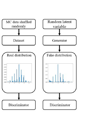
Figure 1: The overall structure of M-WGAN.

Table 1: The structure of the generator for M-WGAN.

Layer (type)	Output Shape	Parameter number
Linear-1	[-1, 6400]	6,400
BatchNorm1d-2	[-1, 6400]	12,800
LeakyReLU-3	[-1, 6400]	0
Linear-4	[-1, 100]	640,000
BatchNorm1d-5	[-1, 100]	200
LeakyReLU-6	[-1, 100]	0
Linear-7	[-1, 4]	400
BatchNorm1d-8	[-1, 4]	8
LeakyReLU-9	[-1, 4]	0
Linear-10	[-1, 100]	400
BatchNorm1d-11	[-1, 100]	200
LeakyReLU-12	[-1, 100]	0
Linear-13	[-1, 4]	400
BatchNorm1d-14	[-1, 4]	8
LeakyReLU-15	[-1, 4]	0
Linear-16	[-1, 100]	400
BatchNorm1d-17	[-1, 100]	200
LeakyReLU-18	[-1, 100]	0
Linear-19	[-1, 6400]	640,000
BatchNorm1d-20	[-1, 6400]	12,800
LeakyReLU-21	[-1, 6400]	0
Linear-22	[-1, 1]	6,400

Table 2: The structure of the discriminator for M-WGAN.

Layer (type)	Output Shape	Parameter number
Linear-1	[-1, 64]	128
LeakyReLU-2	[-1, 64]	0
Linear-3	[-1, 3200]	208,000
LeakyReLU-4	[-1, 3200]	0
Linear-5	[-1, 1]	3,201

The structure of the generator for M-WGAN is explained in Tab. 1. The fully connected layers are applied to reshape the input random latent variable with normal distribution. The batch normalization is exerted to improve generation. The structure of the discriminator for M-WGAN is described in Tab. 2. Three layers of fully connected layers are used. All layers use LeakyReLU except for the output layer.

As a result, the M-WGAN can generate the distribution of the topological charge directly to be applied to calculate the topological charge susceptibilities after training. The M-WGAN realize unsupervised generation without labels. In addition, some programs are based on Pytorch[18].

The next part is the preparation of original data. The software Chroma is used to generate configurations of lattice QCD on individual workstation[19]. In order to obtain the topological charge density data, the configurations are computed first with the pseudo heat bath algorithm and is optimized by Wilson flow[5], then topological charge density data can be calculated from the configurations. In detail, the periodic boundary conditions and hot start have been applied and the updating steps are repeated 10 times for the visited link variable because the computation of sum of staples is costly. The Wilson flow step time $\varepsilon_{f}=0.01$ and total number of steps $N_{flow}=600$ are chosen.

The demonstration that the sampled configurations has reached equilibrium is as follows. To detect whether the system has reached equilibrium, it is possible to check a physical quantity starting from cold start and hot start is consistent after a certain MC steps. The average of the plaquette was chosen to study the equilibrium and the mean value of plaquette is defined as

$$\left\langle{\frac{1}{3}ReTr{U_{plaq}}}\right\rangle$$ (8)

It is found from Fig. 2 that the system has reached equilibrium after about 200 sweeps.

Figure 2: The evolution of the average of plaquette under different initial conditions.

Furthermore, it is necessary to calculate the integrated autocorrelation time which is computed by the topological charge in this article. The definition of the autocorrelation function of the physical quantity X between the field configuration i and i+t is

$${C_{X}}\left({{X_{i}},{X_{i+t}}}\right) =\langle({X_{i}}-\left\langle{{X_{i}}}\right\rangle)({X_{i+t}}-\left\langle{{X_{i+t}}}\right\rangle)$$ (9)

$$=\left\langle{{X_{i}}{X_{i+t}}}\right\rangle-\left\langle{{X_{i}}}\right\rangle\left\langle{{X_{i+t}}}\right\rangle.$$

We define $C_{X}\left(t\right)\mathrm{=}C_{X}\left(X_{i},\mathrm{\ }X_{i+t}\right)$ at equilibrium and the normalized autocorrelation function $\Gamma_{X}\left(t\right)=\frac{C_{X}\left(t\right)}{C_{X}\left(0\right)}$. We introduce the integral autocorrelation time as

$${\tau_{X,int}}=\frac{1}{2}+\sum\limits_{t=1}^{N}{{\Gamma_{X}}(t)}.$$ (10)

It is calculated that the integrated autocorrelation time is 0.416 which indicates that each of data can be regarded as independent because of $N/2\tau_{X,\mathrm{\ int\ }}>N$ [5], where a total of 1000 configurations are sampled with intervals of 200 sweeps.

In addition, the static QCD potential is applied to set the scale and can be parameterized by[5]

$$V\left(r\right)=A+\frac{B}{r}+\sigma r.$$ (11)

The Sommer parameter $r_{\mathrm{0}}$ is defined as

$$\left(r^{2}\frac{dV\left(r\right)}{dr}\right)_{r=r_{0}}=1.65,$$ (12)

and the Sommer parameter $\ r_{\mathrm{0}}\mathrm{\ =\ }0.49fm$ is used[20]. The scales are summarized in the Tab. 3.

Table 3: Setting scale through the static QCD potential.

$lattice$	$\beta$	$a[fm]$	$N_{cnfg}$	${r_{0}}/a$	$L[fm]$
$24\times{12}^{3}$	6.0	0.093(3)	1000	5.30(15)	1.11(3)

III Numerical results

First, we show our results of 100 and 300 original data simulated by the MC with Wilson flow. It is found from Fig. 3 that the topological charge Q is obviously concentrated on the integer positions being consistent with the conclusion that the topological charge is an integer in the continuous case mentioned above.It is calculated from the right subplot of Fig. 3 that the quarter of topological charge susceptibility ${\chi_{t}}^{1/4}=191.59\pm 3.82MeV$ when $N_{flow}=600$. For a comparison, ${\chi_{t}}^{1/4}=191\pm 5MeV$ obtained by Refs[15][21]. Moreover, the distribution of the topological charge should be symmetrical about the origin. However, we can find that the symmetry of distribution is poor in the left subgraph of Fig. 3 due to the poor statistics of data. Therefore, it is better to improve the distribution of data by increasing their statistics. In practice, increasing the amount of data for MC simulations will lead to a rapid increase in time cost and storage usage. Luckily, the ML model can almost avoid this problem. Once the ML model is trained, it can immediately generate a corresponding data to improve the accuracy of the results. Next, we will discuss the details of two methods, the MC with Wilson flow and ML with the M-WGAN scheme, as well as apply a mixture of two methods to simulate configurations more efficiently.

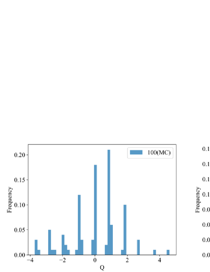
Figure 3: The distribution of topological charge based on the MC with Wilson flow. A total number of Wilson flow time steps $N_{flow}=600$ are chosen. The configuration numbers for calculating topological charge data are 100 for the left subplot and 300 for the right subplot.

For MC, we simulated a total of 1600 configurations and calculated the topological charge from the configurations. Then the quarter of the topological charge susceptibility ${\chi_{t}}^{1/4}=190.84\pm 0.54MeV$ was calculated from 1600 topological charge data and details of the calculations are shown in Tab. 4, when 25 CPU cores were used in our calculations.

For ML, we concern to apply M-WGAN to generate the topological charge data based on the original MC training data. At first, we need to determine how much training data to be suitable. We tested the training processes with training data volumes of 100, 200 and 300 by randomly selecting three-quarters of the data each time to train the model. The distribution of topological charge generated by the model trained using different data volumes is shown in the Fig. 4. It can be observed that the distribution of the middle subgraph is mainly concentrated at the integers compared with the left subgraph, but its peak of the distribution dose not appears at the origin. Furthermore, the distribution of the subgraph on the right is mainly concentrated at the integers and roughly symmetrical about the origin. Therefore, it is found that the model trains better as the amount of training data increases. By the experiences, we prefer to use 300 MC data and randomly select three-quarters of 300 data each time for our train scheme.

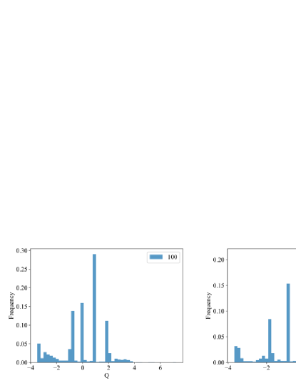
Figure 4: Comparison of models with 100, 200, 300 training data.

For our study, the most important thing we noticed is the accuracy of the physics results for two methods. It can be found from Tab. 4 and Fig. 5 that the data error gradually decreases as size of data increases for both MC and ML, where 300 training data were used to train M-WGAN and then 1600 output data were obtained. In calculations we divide each data into 4 groups, then use the jack-knife to analysis the error for each group and calculate the total error for groups.

When we compare the methods of MC and ML, it is found that the error of the data by ML is consistent with that by MC. And the ML after train can generate data faster and take up less storage space than MC as shown in Tab. 5, where the data volume of MC and ML is both 1600. The time consumption and storage of MC will change proportionally with the size of data volume, but these of ML will hardly change. Therefore, we can apply ML to generate suitable data based on MC data to deal with the error more efficiently.

Furthermore, the distributions of topological charges generated by the MC and ML methods are shown in Fig. 6. It can be observed that both the distributions have good symmetry, and their data are discretely distributed at integers. These characteristics are consistent with the nature of the topological charge. In addition, the integrated autocorrelation time of 1600 data for ML is 0.41, which indicates that these data are independent.

Table 4: The quarter of the topological charge susceptibility ${\chi_{t}}^{1/4}$ for MC and ML.

Data volume	${\chi_{t}}^{1/4}(MC)/MeV$	${\chi_{t}}^{1/4}(ML)/MeV$
400	$191.09\pm 2.65$	$191.38\pm 1.86$
600	$189.34\pm 1.71$	$190.37\pm 1.28$
800	$190.52\pm 1.18$	$191.42\pm 1.09$
1000	$191.20\pm 0.91$	$190.65\pm 0.86$
1200	$191.13\pm 0.73$	$191.61\pm 0.73$
1400	$191.46\pm 0.63$	$191.64\pm 0.62$
1600	$190.84\pm 0.54$	$190.99\pm 0.53$

Figure 5: The quarter of the topological charge susceptibility ${\chi_{t}}^{1/4}$ for MC and ML under different data size.

Table 5: The time consumption and hard disk storage usage for MC and ML. The time and storage of ML incorporate the effects of training data.

Method	Time/h	Storage/MB	${\chi_{t}}^{1/4}/MeV$
MC	136	18230	$190.84\pm 0.54$
ML	26	3423	$190.99\pm 0.53$

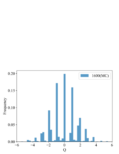
Figure 6: The distributions of topological charge for MC and ML.

IV Conclusion

In this paper, the topological quantities of lattice QCD have been studied by a MC simulation mixed with the M-WGAN. Then we have applied the M-WGAN to generate the distribution of topological charge to show the potential for applications of ML technique in lattice QCD.

By our experience, the conclusions are as follows. Compared with the MC by the pseudo heat bath algorithm and the Wilson flow, our M-WGAN scheme shows its efficiency for the MC simulations in terms of time cost and storage as shown in Tab. 4 and Tab. 5. The data generated by the M-WGAN trained with 300 data are consistent with the corresponding data by the MC simulation as the topological charge susceptibility is concerned. The pseudo distribution generated by this model after a necessary train can be applied to calculate the correct topological charge susceptibility in the SU(3) lattice QCD.

We hope that the M-WGAN can be applied to study other physics problems in the lattice QCD to help us for simulating some interesting quantities more efficiently.

Acknowledgments. This work was done based on the Chroma applied to simulate the configuration of the lattice gauge field. We are grateful to the relevant contributors to the Chroma.

References

- Carrasquilla and Melko [2017] J. Carrasquilla and R. G. Melko, Nature Physics 13, 431 (2017).
- Goodfellow et al. [2014] I. Goodfellow, J. Pouget-Abadie, M. Mirza, B. Xu, D. Warde-Farley, S. Ozair, A. Courville, and Y. Bengio, in Advances in Neural Information Processing Systems, Vol. 27, edited by Z. Ghahramani, M. Welling, C. Cortes, N. Lawrence, and K. Weinberger (Curran Associates, Inc., 2014).
- Goodfellow et al. [2020] I. Goodfellow, J. Pouget-Abadie, M. Mirza, B. Xu, D. Warde-Farley, S. Ozair, A. Courville, and Y. Bengio, Communications of the ACM 63, 139 (2020).
- Wilson [1974] K. G. Wilson, Phys. Rev. D 10, 2445 (1974).
- Gattringer and Lang [2010] C. Gattringer and C. B. Lang, Quantum chromodynamics on the lattice, Vol. 788 (Springer, Berlin, 2010).
- Nicoli et al. [2021] K. A. Nicoli, C. J. Anders, L. Funcke, T. Hartung, K. Jansen, P. Kessel, S. Nakajima, and P. Stornati, Phys. Rev. Lett. 126, 032001 (2021).
- Singha et al. [2023] A. Singha, D. Chakrabarti, and V. Arora, Phys. Rev. D 107, 014512 (2023).
- Nagai et al. [2023] Y. Nagai, A. Tanaka, and A. Tomiya, Phys. Rev. D 107, 054501 (2023).
- Georgi and Politzer [1976] H. Georgi and H. D. Politzer, Phys. Rev. D 14, 1829 (1976).
- ’t Hooft [1986] G. ’t Hooft, Phys. Rept. 142, 357 (1986).
- Atiyah and Singer [1971] M. F. Atiyah and I. M. Singer, Annals of Mathematics 93, 139 (1971).
- Belavin et al. [1975] A. A. Belavin, A. M. Polyakov, A. S. Schwartz, and Y. S. Tyupkin, Phys. Lett. B 59, 85 (1975).
- Witten [1979] E. Witten, Nuclear Physics B 156, 269 (1979).
- Reuter [1997] M. Reuter, Modern Physics Letters A 12, 2777 (1997).
- Lüscher [2010] M. Lüscher, Journal of High Energy Physics 2010, 10.1007/jhep08(2010)071 (2010).
- Moran et al. [2011] P. J. Moran, D. B. Leinweber, and J. Zhang, Phys. Lett. B 695, 337 (2011), arXiv:1007.0854 [hep-lat] .
- Arjovsky et al. [2017] M. Arjovsky, S. Chintala, and L. Bottou, arXiv preprint arXiv:1701.07875 (2017), arXiv:1701.07875 [stat.ML] .
- Paszke et al. [2019] A. Paszke, S. Gross, F. Massa, A. Lerer, J. Bradbury, G. Chanan, T. Killeen, Z. Lin, N. Gimelshein, L. Antiga, et al., Advances in neural information processing systems 32 (2019).
- Edwards and Joó [2005] R. G. Edwards and B. Joó, Nuclear Physics B - Proceedings Supplements 140, 832 (2005).
- Sommer [2014] R. Sommer, arXiv preprint arXiv:1401.3270 (2014).
- Del Debbio et al. [2005] L. Del Debbio, L. Giusti, and C. Pica, Physical review letters 94, 032003 (2005).