Functional upper limits

Abstract

Upper limits and confidence intervals are a convenient way to present experimental results. With modern experiments producing more and more data, it is often necessary to reduce the volume of the results. A common approach is to take a maximum over a set of upper limits, which yields an upper limit valid for the entire set. This, however, can be very inefficient. In this paper we introduce functional upper limits and confidence intervals that allow to summarize results much more efficiently. An application to upper limits in all-sky continuous gravitational wave searches is worked out, with a method of deriving upper limits using linear programming.

I Introduction

Many modern experiments and surveys produce large amounts of data, whose dimensionality keeps increasing. One way to reduce the storage requirements is to employ data compression. However, lossless compression is often only moderately effective, while lossy compression can make upper limits (and confidence intervals in general) invalid.

What is needed is way to perform lossy compression while retaining the validity of upper limits and confidence intervals. This is clearly possible by computing maxima and minima of upper and lower bounds, however this can result in overly inefficient limits.

A better way is to generalize the single value produced by taking a maximum or minimum to a function given by a formula with a few coefficients. The coefficients are optimized to minimize error, while the function is required to always be conservative with regard to the limit or confidence interval being approximated.

In the following section we give a formal definition of a functional upper limit, and then describe in detail construction and performance of functional upper limits produced for the atlas of continuous gravitational waves.

II Functional compression

Suppose our search has computed upper limits $\textrm{UL}=\textrm{UL}(x)$ as a function of variable $x\in X$.

To compress the data, we pick a set of functions $\left\{\widehat{\textrm{UL}}\left(x;\vec{c}\right)\right\}$. Then the goal of a compression algorithm is to find parameter $\vec{c}$ such that the compressed form is always at or above original upper limit data:

$$\forall x\in X:\widehat{\textrm{UL}}\left(x;\vec{c}\right)\geq\textrm{UL}\left(x\right)$$ (1)

while minimizing error

$$\max_{x\in X}\left(\widehat{\textrm{UL}}\left(x;\vec{c}\right)-\textrm{UL}\left(x\right)\right)\rightarrow\min$$ (2)

The choice of error function is somewhat arbitrary. It is often a good idea to pick an error function that makes the optimization problem easy to compute. The compression of lower limits is done in the same way, by simply inverting the sign. Confidence intervals can be compressed by treating lower and upper bounds separately.

There is an efficient way to compute optimal function $\widehat{\textrm{UL}}$. To begin, suppose we pick a set of constant functions $\left\{c:c\in{\mathbb{R}}\right\}$. Then the compression algorithm can compute

$$\widehat{\textrm{UL}}=\max_{x}\textrm{UL}\left(x\right)$$ (3)

This clearly satisfies the validity constraint given by Eqn. 1 and is easy to compute. However, the error equals to the range of upper limit values.

We can improve the performance by introducing more coefficients:

$$\widehat{\textrm{UL}}(x)=h\left(\frac{\vec{c}\cdot\vec{f}\left(x\right)}{g(x)}\right)$$ (4)

where $h$ is an increasing monotonic invertible function and $\vec{f}$ and $g$ are some suitable functions of $x$.

Then the problem of finding optimal coefficients $\vec{c}$ can be framed as a linear programming problem:

$$\left\{\begin{array}[]{l}h^{-1}\left(\textrm{UL}(x)\right)g(x)\leq\vec{c}\cdot\vec{f}(x)\\ \underset{x\in X}{\max}\left(\frac{\vec{c}\cdot\vec{f}\left(x\right)}{g(x)}-h^{-1}\left(\textrm{UL}(x)\right)\right)\rightarrow\min\end{array}\right.$$ (5)

as long as we are willing to modify the error function (eqn. 2) to compute the error in $h^{-1}\left(\textrm{UL}\right)$.

Theoretically, this data compression can be very effective because we replace a large vector of values $\left(\textrm{UL}(x):x\in X\right)$ with much smaller number of coefficients $\vec{c}$. And since coefficients $\vec{c}$ can be found with a linear programming algorithm, it is feasible to apply this technique to large volumes of data, with functional upper limits computed repeatedly for different inputs $\textrm{UL}(x)$.

We will now describe how functional upper limits are applied to construct an atlas of continuous gravitational waves.

III All-sky searches for continuous gravitational waves

All-sky searches for continuous gravitational waves produce vast amounts of data [1, 2, 3, 4, 5, 6, 7, 8, 9]. These searches are looking for unknown gravitational wave sources by sweeping large parameter spaces. Of course, most of the parameter space does not contain signals loud enough to be detected. In this case, the search places an upper limit on possible signal strength.

Reporting these upper limits can be problematic because of large number of dimensions - a relatively simple search will have two dimensions for the sky, one for frequency and two for polarization. Allowing additional parameters, such as frequency derivative or binary evolution of the source, increases dimensionality further.

The technique used in the past to compress the data was to maximize upper limits over a subset of parameter space. For example, a maximum can be computed over polarization and a small range of frequencies.

Reducing polarization data by maximization is far from optimal because there is a large variation in upper limits between linearly and circularly polarized sources, as can be seen in Figure 1.

In this paper we describe how one can report polarization specific upper limits using only a few dozen numbers per record. These numbers define a function of coefficients computed from polarization parameters $\iota$ and $\psi$.

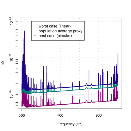
Figure 1: Gravitational wave intrinsic amplitude $h_{0}$ upper limits at 95% confidence as a function of signal frequency [1].

IV Polarizations of gravitational waves

A prototypical source of continuous gravitational waves is a neutron star with equatorial deformation. Such rotating source will emit circularly polarized waves along the rotation axis and linearly polarized wave, perpendicular to the rotation axis.

We start by assuming that our signal consists of two polarizations:

$$\begin{array}[]{rcl}h_{+}^{\prime}&=&A_{+}\cos(\omega t+\phi)\\ h_{\times}^{\prime}&=&A_{\times}\sin(\omega t+\phi)\\ \end{array}$$ (6)

A generic pulsar signal can be represented as $A_{+}=h_{0}\left(1+\cos^{2}(\iota)\right)/2$, $A_{\times}=h_{0}\cos(\iota)$, with $h_{0}=A_{+}+\sqrt{A_{+}^{2}-A_{\times}^{2}}$ and $\cos(\iota)=A_{\times}/\left(A_{+}+\sqrt{A_{+}^{2}-A_{\times}^{2}}\right)$

We will assume that demodulation is performed for a fixed frame of plus and cross polarizations rotated at an angle $\beta$. In this coordinate system we have:

$$\begin{array}[]{rcl}h_{+}&=&A_{+}\cos(\omega t+\phi)\cos(\epsilon)-A_{\times}\sin(\omega t+\phi)\sin(\epsilon)\\ h_{\times}&=&A_{+}\cos(\omega t+\phi)\sin(\epsilon)+A_{\times}\sin(\omega t+\phi)\cos(\epsilon)\\ \end{array}$$ (7)

where $\epsilon=2(\psi-\beta)$. The angle $\psi$ describes polar angle of the source rotation axis to the line of sight. The angle $\beta$ is important when performing analysis because the detector orientation changes with time. For reporting results, we can simply pick any convenient frame, so for the rest of the paper we assume $\beta=0$.

Continuous wave searches usually do not use high sample rate data. Rather, a set of short Fourier transforms (SFTs) is computed, and the search loads only the bins covering the frequency band of interest. The Fourier transforms are picked to be short enough so that the Doppler modulation from Earth motion is negligible. The signal amplitude in SFT bin corresponding to frequency $\omega$ is then

$$\begin{array}[]{rcl}z&=&\displaystyle\int\left(F_{+}h_{+}+F_{\times}h_{\times}\right)e^{-i\omega t}dt=\\ &=&\vphantom{\int}\frac{1}{2}e^{i\phi}\left(F_{+}(A_{+}\cos(\epsilon)+iA_{\times}\sin(\epsilon))+\right.\\ &&\qquad\left.+F_{\times}(A_{+}\sin(\epsilon)-iA_{\times}\cos(\epsilon))\right)\\ &=&F_{+}w_{1}+F_{\times}w_{2}\end{array}$$ (8)

where we introduced complex amplitude parameters

$$\begin{array}[]{rcl}w_{1}&=&\frac{1}{2}e^{i\phi}(A_{+}\cos(\epsilon)+iA_{\times}\sin(\epsilon))\\ w_{2}&=&\frac{1}{2}e^{i\phi}(A_{+}\sin(\epsilon)-iA_{\times}\cos(\epsilon))\\ \end{array}$$ (9)

The complex amplitude parameters $w_{1}$ and $w_{2}$ are algebraically symmetric, and satisfy the following equation of constant $h_{0}$:

$$\sqrt{|w_{1}+iw_{2}|}+\sqrt{|w_{1}-iw_{2}|}=\sqrt{h_{0}}$$ (10)

the solutions of which form a singular surface enclosing a non-convex solid. This complicated form is responsible for differences between worst-case circular upper limits, population average upper limits, and circularly polarized upper limits.

The normalized complex parameters are introduced by setting $\tilde{w}_{1}=w_{1}/h_{0}$ and $\tilde{w}_{2}=w_{2}/h_{0}$, and satisfy the equation:

$$\sqrt{|\tilde{w}_{1}+i\tilde{w}_{2}|}+\sqrt{|\tilde{w}_{1}-i\tilde{w}_{2}|}=1$$ (11)

V Construction of functional upper limits

The polarization dependence of upper limits is described by a function on two-dimensional space $x=(\iota,\psi)$.

We pick $h(v)=\sqrt{v}$, thus we measure error in the square of the upper limit value. The vector $\vec{c}$ has 14 components $c_{1-14}$. Our upper limits model $\widehat{\textrm{UL}}$ is then a square root of a rational function of trigonometric functions of $\iota$ and $\psi$:

$$\begin{array}[]{l}\widehat{\textrm{UL}}^{2}=\left(c_{1}+f_{pp}c_{2}+f_{pc}c_{3}+f_{cc}c_{4}+f_{impc}c_{5}+f_{pp}^{2}c_{6}+\right.\\ \quad\quad\quad\left.+f_{cc}^{2}c_{7}+f_{pc}^{2}c_{8}+f_{impc}f_{pp}c_{9}+f_{impc}f_{pc}c_{10}+\right.\\ \quad\quad\quad\left.+f_{impc}f_{cc}c_{11}+f_{pp}f_{pc}c_{12}+f_{cc}f_{pc}c_{13}+\right.\\ \quad\quad\quad\left.+f_{pp}f_{cc}c_{14}\right)/\left(f_{pp}+f_{cc}\right)\end{array}$$ (12)

where coefficients $f_{\cdot}=f_{\cdot}(\iota,\psi)$ are given by the following formulas:

$$\begin{array}[]{ll}a_{+}&=\frac{\left(1+\cos^{2}\iota\right)^{2}}{4}\\ a_{\times}&=\cos^{2}\iota\\ f_{pp}&=2|\tilde{w}_{1}|^{2}=\frac{1}{4}\left(a_{+}+a_{\times}+\left(a_{+}-a_{\times}\right)\cos 4\psi\right)\\ f_{pc}&=4\textrm{Re}\,\tilde{w}_{1}\tilde{w}_{2}^{*}=\frac{1}{2}\left(\left(a_{+}-a_{\times}\right)\sin 4\psi\right)\\ f_{cc}&=2|\tilde{w}_{2}|^{2}=\frac{1}{4}\left(a_{+}+a_{\times}-\left(a_{+}-a_{\times}\right)\cos 4\psi\right)\\ f_{impc}&=2\textrm{Im}\,\tilde{w}_{1}\tilde{w}_{2}^{*}=\frac{1}{4}\left(1+\cos^{2}\iota\right)\cos\iota\end{array}$$ (13)

The denominator of equation 12 helps to compress the range of upper limits, while coefficients $c_{1-14}$ allow sufficient freedom to bring upper limit overestimate under 5% for most data.

The coefficients $c_{1-14}$ can be found using the following linear optimization problem:

$$\left\{\begin{array}[]{l}\textrm{UL}^{2}\left(f_{pp}+f_{cc}\right)\leq c_{1}+f_{pp}c_{2}+f_{pc}c_{3}+f_{cc}c_{4}+\\ \quad\quad\quad+f_{impc}c_{5}+f_{pp}^{2}c_{6}+f_{cc}^{2}c_{7}+f_{pc}^{2}c_{8}+\\ \quad\quad\quad+f_{impc}f_{pp}c_{9}+f_{impc}f_{pc}c_{10}+f_{impc}f_{cc}c_{11}+\\ \quad\quad\quad+f_{pp}f_{pc}c_{12}+f_{cc}f_{pc}c_{13}+f_{pp}f_{cc}c_{14}\\ \textrm{UL}^{2}\left(f_{pp}+f_{cc}\right)\geq c_{1}+f_{pp}c_{2}+f_{pc}c_{3}+f_{cc}c_{4}+\\ \quad\quad\quad+f_{impc}c_{5}+f_{pp}^{2}c_{6}+f_{cc}^{2}c_{7}+f_{pc}^{2}c_{8}+\\ \quad\quad\quad+f_{impc}f_{pp}c_{9}+f_{impc}f_{pc}c_{10}+f_{impc}f_{cc}c_{11}+\\ \quad\quad\quad+f_{pp}f_{pc}c_{12}+f_{cc}f_{pc}c_{13}+f_{pp}f_{cc}c_{14}+\\ \quad\quad\quad+uw\\ u\rightarrow\min\end{array}\right.$$ (14)

here UL, $f_{\cdot}$ and $w$ are functions of $\iota$ and $\psi$, typically taken from precomputed grid. After optimization, a correction can be applied that compensates for grid spacing and assures that upper limits $\tilde{\textrm{UL}}$ are valid for any $\iota$ and $\psi$.

There are many existing linear programming algorithms capable of solving model 14, for example various simplex algorithms and interior point methods. As the model has few variables, it appears particularly simple.

One implementation quirk that makes things interesting is that practical implementations of these algorithms often encounter difficulties on some subset of inputs. For example, simplex algorithms can loop and/or fail to converge due to ill-conditioned matrices that define the problem.

In many situations, this is not a big problem as the input data can be slightly perturbed. However, the all-sky searches such as Falcon [1] need to find coefficients $c_{1-14}$ for billions of models, which input data, UL, is derived from noise.

This practically guarantees that a weak point of any particular linear optimization algorithm will be encountered during the analysis. The solution we have chosen is to try different optimization algorithms one after another with a time limit within which they are expected to converge. Finally, if none of these succeed we settle for a solution of 14 that is valid, but not necessarily optimal.

VI Application example

To test our technique, we implemented it as part of a Falcon search and then carried out a search on data with software injections. The 31574 injections were uniformly distributed in the sky, with frequency derivatives from 0 to ${-5}{\times 10^{-10}}$ Hz/s, and polarizations distributed assuming random source orientations.

Figure 2 shows how upper limits established by Falcon pipeline compare with injection strength. To be correct, the upper limit has to be above the $y=x$ line marked in red.

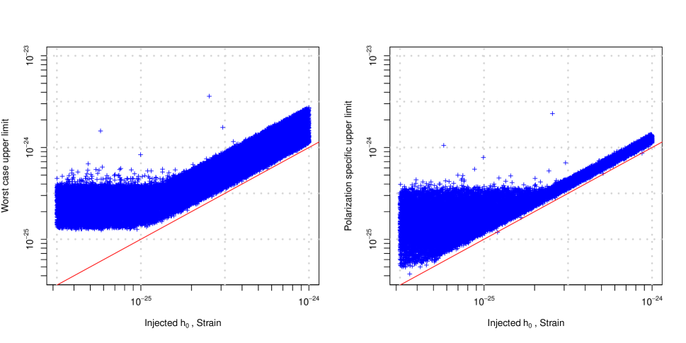
Figure 2: Upper limit versus injected strain for a set of software injections [1]. The left graph shows worst case upper limit, while the right plot shows polarization specific upper limit computed using $\iota$ and $\psi$ used to inject signals.

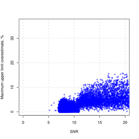
Figure 3: Estimate of relative upper limit error versus SNR of software injection. For injections with small SNR the worst case error is around 5%, for stronger injections it can be much larger.

The left plot shows conventional worst-case upper limit. We see a fairly wide spread above the red line, which happens because some injections are circularly polarized and deliver a lot more power.

The right plot shows polarization specific upper limit. To produce it, the Falcon pipeline first compressed the data to produce a functional upper limit, and then that function was evaluated for $\iota$ and $\psi$ that were used to make the injection. We see that polarization specific upper limits have a far smaller spread for loud injections as they are more accurate.

For very weak injections the injected signals are dominated by detector noise. Here, polarization specific upper limits show their main benefit as they can rigorously establish far lower upper limits for elliptically polarized signals. Indeed, the spread of blue points extends far below $10^{-25}$.

Figure 3 shows how relative error in the upper limit depends on the injection strength. The functional model has been optimized for the noise dominated case. There we overestimate upper limits by 5% or less. As injection SNR grows, our model becomes less efficient. This is not a big problem because for SNRs that large the Falcon pipeline can easily recover astrophysical signals.

VII Conclusions

We have described a new method that allows to establish upper limits and confidence intervals as a function, rather than a single number. This method has been successfully used to compress Falcon atlas of continuous gravitational waves, where for the first time, we were able to provide upper limits for all polarizations. The functional upper limits are established by linear optimization that, in rare cases, presents difficulties for conventional linear optimization codes. It would be interesting to explore whether a more efficient optimizer can be constructed to solve the model of the form 14.

References

- [1] Vladimir Dergachev and Maria Alessandra Papa, Frequency-Resolved Atlas of the Sky in Continuous Gravitational Waves, Phys. Rev. X 13, 021020 (2023)
- [2] Vladimir Dergachev and Maria Alessandra Papa, Early release of the expanded atlas of the sky in continuous gravitational waves, arXiv: XXXXX (2023)
- [3] V. Dergachev, M. A. Papa, Results from the first all-sky search for continuous gravitational waves from small-ellipticity sources, Phys. Rev. Lett. 125, no.17, 171101 (2020)
- [4] V. Dergachev, M. A. Papa, Results from high-frequency all-sky search for continuous gravitational waves from small-ellipticity sources, Phys. Rev. D 103, 063019 (2021)
- [5] V. Dergachev, M. A. Papa, The search for continuous gravitational waves from small-ellipticity sources at low frequencies, Phys. Rev. D 104, 043003 (2021)
- [6] K. Riles, Searches for Continuous-Wave Gravitational Radiation, Living Reviews in Relativity 26, 3 (2023)
- [7] B. Steltner, M. A. Papa, H. B. Eggenstein, R. Prix, M. Bensch, B. Allen and B. Machenschalk, Deep Einstein@Home All-sky Search for Continuous Gravitational Waves in LIGO O3 Public Data, Astrophys. J. 952, no.1, 55 (2023)
- [8] R. Abbott et al.(LIGO Scientific Collaboration, Virgo Collaboration and KAGRA Collaboration), All-sky search for continuous gravitational waves from isolated neutron stars in the early O3 LIGO data, Phys. Rev. D 104, 082004 (2021)
- [9] R. Abbott et al.(LIGO Scientific Collaboration, Virgo Collaboration and KAGRA Collaboration), All-sky search for continuous gravitational waves from isolated neutron stars using Advanced LIGO and Advanced Virgo O3 data, Phys. Rev. D 106, 102008 (2022)