JADES: Carbon enrichment 350 Myr after the Big Bang in a gas-rich galaxy

Finding the emergence of the first generation of metals in the early Universe, and identifying their origin, are some of the most important goals of modern astrophysics. We present deep /NIRSpec spectroscopy of , a galaxy at z=12.5, in which we report the detection of C iii]1907,1909 nebular emission. This is the most distant detection of a metal transition and the most distant redshift determination via emission lines. In addition, we report tentative detections of [O ii]3726,3729 and [Ne iii]3869, and possibly O iii]1661,1666. By using the accurate redshift from C iii], we can model the Ly drop to reliably measure an absorbing column density of hydrogen of $\NHI\approx 10^{22}\leavevmode\nobreak\ \percm{-2}$ – too high for an IGM origin and implying abundant ISM in or CGM around it. We infer a lower limit for the neutral gas mass of about $10^{7}\leavevmode\nobreak\ M_{\odot}$ which, compared with a stellar mass of $\sim 4\times 10^{7}\leavevmode\nobreak\ M_{\odot}$ inferred from the continuum fitting, implies a gas fraction higher than about 0.1–0.5. We derive a solar or even super-solar carbon-to-oxygen ratio, tentatively $\CO>0.15$. This is higher than the C/O measured in galaxies discovered by at $z=6\text{--}9$, and higher than the C/O arising from Type-II supernovae enrichment, while AGB stars cannot contribute to carbon enrichment at these early epochs and low metallicities. Such a high C/O in a galaxy observed 350 Myr after the Big Bang may be explained by the yields of extremely metal poor stars, and may even be the heritage of the first generation of supernovae from Population III progenitors.

1 Introduction

The appearance of the first galaxies marks a key phase transition of the Universe, i.e. the end of the dark ages. A keystone of this phase transition is the start of stellar nucleosynthesis and the diffusion of metals. Extensive theoretical work has been devoted to predicting the properties of the first generation of stars (Population III, hereafter: PopIII; e.g., Hirano et al., 2014) and their supernova yields (Heger & Woosley, 2010; Limongi & Chieffi, 2018). While PopIII stars are thought to be short-lived (with typical masses of 10–40 ; Hosokawa et al., 2011), the chemical ‘signature’ of their yields may be still observable today. Empirically, extensive searches of PopIII-enriched systems have been undertaken both within the Milky Way (e.g., Frebel & Norris, 2015) and in extragalactic absorbers, including both the most metal-poor damped Ly (DLA) systems (e.g., Pettini et al., 2008; Salvadori & Ferrara, 2012; Cooke et al., 2017; Saccardi et al., 2023) and Lyman-limit systems (LLS; Fumagalli et al., 2016; Saccardi et al., 2023).

The launch of enabled, for the first time, the measurement of the physical properties of galaxies out to z$>$10 (Curtis-Lake et al., 2023; Robertson et al., 2023; Bunker et al., 2023b; Tacchella et al., 2023; Maiolino et al., 2023; Arrabal Haro et al., 2023; Hsiao et al., 2023). These high-redshift observations challenge the extrapolation of trends derived at lower redshifts. These are generally understood in terms of decreasing gas metallicity (Schaerer et al., 2022; Curti et al., 2023b; Nakajima et al., 2023) and increasing density (Reddy et al., 2023), ionisation parameter (Cameron et al., 2023b), temperature (Curti et al., 2023a) and stochasticity of their star-formation histories (SFH; Dressler et al., 2023; Endsley et al., 2023; Looser et al., 2023). However, extrapolations of these trends at z$>$10 do not fully explain the observed properties of galaxies. One reason is that as our observations approach the end of ‘Cosmic Dawn’ (150–250 Myr after the Big Bang, Robertson, 2022), galaxies may carry stronger imprints from the first generation of metal-poor stars, whose physical properties and spectra are poorly understood. Most notably, nebular emission-line ratios in a luminous galaxy at $z=10.6$ (GN-z11, Oesch et al., 2016; Bunker et al., 2023b) seem to require exotic chemical abundances (Cameron et al., 2023a), or proto-globular clusters (Senchyna et al., 2023), or Wolf-Rayet stars – possibly with a fine-tuned SFH (Kobayashi & Ferrara, 2023). Moreover, a supermassive accreting black hole has been identified in this galaxy, suggesting that the peculiar chemical abundances might be primarily associated with its nuclear region (Maiolino et al., 2023).

In addition to rare objects like the remarkably bright GN-z11, enabled the observations of spectra of regular galaxies at $z=10\text{--}13$ Curtis-Lake et al., 2023, hereafter: ; Hsiao et al., 2023; Arrabal Haro et al., 2023, at redshifts even higher than GN-z11, i.e., even nearer to the end of Cosmic Dawn. While less extreme than objects like GN-z11, these galaxies are more representative of the typical physical properties of galaxies at those epochs , Robertson et al., 2023. One of the remarkable findings of was the lack of any emission lines – even with the unprecedented depth of the Advanced Deep Extragalactic Survey (JADES; Eisenstein et al., 2023b; Rieke et al., 2023; Bunker et al., 2023a). Unfortunately, the lack of emission lines severely affects our ability to constrain the physical properties and chemical abundances of these galaxies, because systematic uncertainties dominate the constraints introduced through strong priors on, e.g., the shape of the SFH as well as other factors; .

To address this shortcoming, the large programme PID 3215 (Eisenstein et al., 2023a), while obtaining deep multi-band imaging, has in parallel also obtained the deepest spectroscopic observations yet of galaxies at $z>10$, thanks to a 50-hours integration with /NIRSpec, for a 5-emission-line sensitivity of $10\text{--}5\times\fluxcgs[-20]$ at $\approx 2\text{--}5\leavevmode\nobreak\ \mum$ (for spectrally unresolved lines). In this article, we report the first analysis of the new spectroscopic data for , a $z>10$ galaxy already analysed in and Robertson et al. (2023). After presenting the data reduction and analysis in § 2, we show the physical constraints obtained from the data (§ 3-5) and conclude with a brief discussion and outlook (§ 6).

Throughout this work, we assume the Planck Collaboration et al. (2020) cosmology, a Chabrier (2003) initial mass function (IMF) with an upper-mass cutoff of 300 , and the Solar abundances of Asplund et al. (2009). Stellar masses refer to the total stellar mass formed (i.e., the integral of a galaxy SFH), and distances are proper distances.

2 Observations, sample and data analysis

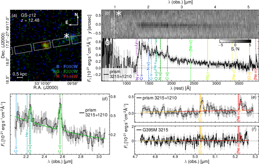
Figure 1: Panel 1; false-colour RGB image, highlighting the position of the NIRSpec/MSA shutters in PID 3215. The asterisk indicates the position of an interloper with low surface brightness, which was removed in the data reduction. Panel 1; 2-d S/N map, showing the three central shutters (the asterisk is the position of the interloper). Panel 1; 1-d boxcar-extracted prism spectrum, combining 3215 and 1210; the vertical dashed lines marking the position of strong emission lines at $z=\zspec$. Panels 1–1; combined 3215 and 1210 data and model spectrum around the O iii], C iii], [O ii] and [Ne iii] lines, for the prism (panels 1 and 1) and for the G395M grating (only 3215; panel 1). C iii] is detected at the 5-level (7-with the bootstrapping method). O iii] is not robustly detected (2.3-significance); [O ii] and [Ne iii] are marginally detected only in the prism (4- and 3.5-) but not in the grating, despite comparable sensitivity. The vertical dashed lines mark the wavelength of the emission lines at the redshift of the object, with the shaded region indicating the redshift uncertainty.

The observations consist of NIRSpec Micro-Shutter Assembly (MSA) spectroscopy with the prism and with the G140M and G395M gratings. These data were obtained as part of programmes PID 1210 PI N. Lützgendorf; already presented in and Bunker et al., 2023a and PID 3215 PI D. Eisenstein and R. Maiolino, Eisenstein et al., 2023a. A summary of the observing configurations and total integrations is provided in Table 1. The data reduction was performed exactly as described in Bunker et al. (2023a); Carniani et al. (2023). We used nodding for background subtraction, and extracted the 1-d spectrum using a 3-pixel window. Effective line spread functions (LSF) were obtained from modelling the instrument, as described in de Graaff et al. (2023). The input model for each galaxy was obtained from forcepho (Johnson et al., in prep.), using the same methods as described in Baker et al. (2023). The results are shown in Table 2. We applied a slit-loss correction appropriate for point sources (cf. the morphological parameters reported in Table 2). We note that this slit-loss correction is optimised for a 5-pixel aperture. For the analysis, we combine the data from PIDs 3215 and 1210 using a simple inverse-variance weighting.

Summary of the observations from programmes 1210 and 3215. Disperser prism G140M G395M Filter CLEAR F070LP F290LP Spectral resolution $R$ 30–300 700–1500 700–1500 Exp. time 1210 [h] 18.7 4.7 4.7 Exp. time 3215 [h] 46.7 11.7 46.7 (37.4)^‡ Exp. time Total [h] 65.4 16.4 51.5 (42.1)^‡

Table 1: These exposure times apply only to ; other targets in the two programmes may have different exposure times, depending on the mask allocation. ^‡ The last visit was affected by short circuits, and the true exposure time in PID 3215 is reduced to 37.4 h.

In the left column of Fig. 1 we display NIRCam imaging for (panel 1), with overlaid the configuration of the NIRSpec MSA shutters in PID 3215 (these observations consist of five dithered pointings). The 2-d signal-to-noise ratio (S/N) and the boxcar extracted 1-d spectrum are shown in panels 1 and 1.

Panel 1 shows a contaminant with low surface brightness to the west (marked by an asterisk). This contaminant also appears at the top of the 2-d S/N map (panel 1), and its presence was taken into account in the data reduction. Nevertheless, for the prism data of 3215, we measured a negative flux blueward of the Ly drop. The origin of this artefact is still unclear. To remove it, we extracted two background spectra from the 2-d spectrum (above and below the object trace), fitted a declining exponential to these data, and removed the average best-fit background model from the 1-d spectrum. This procedure has no detectable impact on the emission-line fluxes, but affects the shape of the continuum and Ly drop. The uncertainties from the data reduction pipeline were validated by inspecting the dispersion of the individual integrations in each wavelength channel (Appendix A). Overall, we find that the data-reduction pipeline gives more conservative noise estimates than bootstrapping, which is expected because bootstrapping does not take into account correlated noise.

2.1 Emission-line fitting

Emission-line fluxes and equivalent widths (EW) were measured using a local pixel-integrated Gaussian model with linear background, in a window of 0.3 on either side of the expected line location. The lines were assumed to be spectrally unresolved (Gaussian equal to one spectral pixel). The model has four free parameters: flux, redshift, and two coefficients for the background. The redshift was constrained to be centred at $z=12.479$ using a Gaussian prior with dispersion set to 0.014 (this redshift dispersion is the uncertainty we derived from the redshift estimate, see § 2.2). The fiducial values and uncertainties were estimated using a Markov-Chain Monte-Carlo integrator (Foreman-Mackey et al., 2013); the results are reported in Table 3.

The four emission lines O iii]1661,1666, C iii]1907,1909, [O ii]3726,3729 and [Ne iii]3869 (hereafter simply: O iii], C iii], [O ii] and [Ne iii]) are central to our analysis of chemical abundances, and for this reason are measured adopting a different strategy compared to all the other lines. In addition, while O iii] and C iii] are observed only by the prism, [O ii] and [Ne iii] are covered both by the prism and by the G395M grating. Therefore, to take full advantage of the 100-h total integration for [O ii] and [Ne iii], we fit simultaneously the prism and grating spectra. The model uses six pixel-integrated Gaussians, one each for O iii] and C iii] (only present in the prism spectrum), and two each for [O ii] and [Ne iii] (which require separate models for the prism and grating spectra). In total, the model has sixteen free parameters. C iii] has three free parameters (flux, width, and redshift for the prism only); O iii] has two free parameters, flux and redshift for the prism only; its width is constrained to be the same as C iii], and its redshift has a Gaussian prior centred on the C iii] redshift and with $\sigma_{z}=0.02$. [O ii] and [Ne iii] are treated as unresolved, hence have a fixed Gaussian dispersion equal to one spectral pixel (as appropriate for the prism and grating separately). The redshifts of [O ii] are free and independent in the prism and grating, but we apply Gaussian priors of width $\sigma_{z}=0.02$ to maintain them consistent with C iii]. This gives two free parameters (with strong priors). The redshifts of [Ne iii] are the same as for [O ii] in each of the two disperser configurations. For both [O ii] and [Ne iii], the prism flux is a free parameter, while the grating flux is set to the prism flux up-scaled by 11 per cent (to take into account the systematic flux calibration discrepancy between these two observing modes, e.g., Bunker et al., 2023b). In total, we have nine free parameters describing six Gaussian line shapes. We further add seven parameters to model the local background. The background around C iii] and O iii] in the prism is modelled with a 2^nd-order polynomial (three free parameters); the background around [O ii] and [Ne iii] is modelled with a straight line, requiring two parameters each for the prism and for the grating spectrum. The prism spectral resolution and detector sampling prevent us from resolving the two variable-ratio doublets C iii] and [O ii]. We therefore adopt wavelengths of 1,907.71 and 3,728.49 Å, respectively, obtained by averaging the vacuum wavelengths of the two lines in each doublet. Depending on the doublet ratio for C iii] and [O ii], this choice introduces a systematic error of up to 0.1 and 0.4 pixels.

A summary of the emission lines and of their fluxes (or upper limits) is provided in Table 3.

2.2 Detection of C iii]

We adopt a detection threshold of 5 , and report the detection of an emission line at $2.57\leavevmode\nobreak\ \mum$, with a 5-significance. This S/N estimate is based on the conservative uncertainties reported by the data reduction pipeline (bootstrapping the data to estimate the uncertanties would increase the significance to 7 , as discussed in Appendix A). At the redshift initially estimated by from the Ly drop ($z=12.6\pm 0.05$), the line emission at 2.57 is significantly offset (2,600 , i.e. one spectral resolution element) from the expected location of C iii] (the closest emission line; the expected location is highlighted by the vertical dotted line in Fig. 1). However, in addition to the formal significance, other pieces of evidence contribute to confirming that this is a solid detection. The comparison of the two independent datasets 3215 and 1210 (Fig. 6) shows that the line is seen independently, at the expected level of significance, in both observations. The robustness of the line detection is also confirmed by the visual inspection of the 2-d spectrum, in which the line is observed on three pixels in the spatial direction along the slit. Based on these various lines of evidence, we interpret this line as C iii], making it the most distant metal line detection to date.

We measure a high $\text{EW(\text{{C}\,{\sc{iii}}]{}{}{}{}})}=30\pm 7\leavevmode\nobreak\ \AA$. Similarly high EW(C iii]) have been found in some local metal-poor dwarf galaxies, such as ($\mstar\approx 10^{5}\,\MSun$; Kunth et al., 1981; Kumari et al., 2023), considered a local analogue of high-redshift star-forming galaxies, as well as in more massive galaxies at intermediate redshifts ($2<z<4$; Le Fèvre et al., 2019) and at $7<z<9$ (Stark et al., 2017).

With our joint modelling fit, i.e. including the tentative detections of other lines discussed in the next section, we find a redshift of $z=12.482\pm 0.012$. Modelling only C iii] at the mean rest-frame wavelength of 1,907.71 Å, we find $z=12.479\pm 0.014$. In both cases, there is a clear shift with respect to the earlier redshift measurement based off the observed wavelength of the Ly drop (). We interpret this redshift discrepancy as evidence for a high column density of cold gas in the inter-stellar medium (ISM) of , or in its immediate surroundings, whose Ly damping wings affect the Ly drop; this will be further discussed in § 4.

2.3 Additional tentative detections and upper limits

In Table 3 we also report a tentative detection of O iii] (2.3-significance, or 3.5-if adopting the bootstrap method discussed in the Appendix). This line is found at a wavelength consistent with the redshift of C iii], but it is not detected in the 1210 and 3215 observations taken separately (Fig.6).

Similarly, there appears to be a C iv1549,1551 (hereafter: C iv) P-Cygni line at rest-frame 1,550 Å, and a blue-shifted absorption of C ii1334. If confirmed, these might trace a galactic outflow, but the high implied velocities of about 3,000 would require an AGN. On the basis of current data, these features are considered undetected.

Table 3 also reports tentative detections of [O ii] (at 4.4 ) and [Ne iii] (at 3.7 ). Both lines are below the adopted threshold of 5 . In addition to this threshold criterion, we do not consider these lines to be secure detections for the reasons discussed in detail in Appendix A. The arguments in favour of a detection are the correct inter-line wavelength separation, and the combined S/N from the two lines. Yet, several arguments cast doubts about their detection: (i) the moderate (2-) tension between the redshifts of C iii] and [O ii]–[Ne iii] (the dashed vertical lines and shaded region in Fig. 1 show the expected location of these lines given the C iii] redshift and its associated uncertainty). (ii) the unphysical wavelength offset of 2 pixels of [O ii] measured in 1210 with respect to 3215 (cf. cyan and sand lines in Fig. 6). (iii) while [Ne iii] appears in both datasets at the same wavelength, its profile in 1210 appears to be too narrow and is consistent with a noise spike. (iv) visually inspecting the 2-d S/N map (Fig. 1), we find no strong evidence for either [O ii] or [Ne iii] (unlike for C iii], which is clearly visible); [O ii], in particular, appears to originate from a single spaxel, which would be unphysical, because at 5 the point spread function is well sampled by the NIRSpec pixels, so we would expect the line to be spatially extended (like C iii]).

The above difficulties with the 4- and 3-tentative detections justify our choice of a 5-detection threshold. Based on this value, we only consider the C iii] detection as solid. We adopt 3-upper limits (99.9 per cent confidence) on C iv, [O ii] and [Ne iii]. Nevertheless, promoting [O ii] and [Ne iii] to detections would not alter our conclusions. To help the reader judge the effect of assuming both [O ii] and [Ne iii] to be detected, where relevant we report the results when assuming detections, marking them with a small $\dagger$ symbol (Figs 4 and 5).

Physical parameters of .
[arcsec] $0.040\pm 0.003$ P.A. [degree] $70\pm 6$ axis ratio $q$ — $0.55\pm 0.07$ Sérsic index — $0.90\pm 0.09$ $\log\,\mstar$ [] $7.64\pm 0.15$ SFR [ ] $1.15\pm 0.15$ — $0.12\pm 0.04$ [] $7.9\pm 0.2$

Table 2: photometry was obtained as explained in Baker et al. (2023). The setup is described in § 3.

Nebular emission lines for . Line(s) Flux EW PRISM N iv]1486 $<3.3$ $<6.4$ C iv1549,1551 $<3.3$ $<5.5$ He ii1640 $<2.6$ $<4.2$ O iii]1661,1666 ^‡ $(6.0\pm 2.6)$ $8\pm 3$ N iii]1747–1754 $<2.2$ $<3.8$ C iii]1907,1909 ^‡ $\mathbf{12.4\pm 2.5}$ $\mathbf{30\pm 7}$ [Ne iv]2422,2424 $<1.0$ $<3.9$ Mg ii2796,2803 $<0.8$ $<4.6$ [Ne v]3426 $<1.0$ $<8.6$ [O ii]3726,3729 ^‡ $(3.5\pm 0.8)$ $41\pm 12$ [Ne iii]3869 ^‡ $(3.3\pm 0.9)$ $39\pm 13$ G140M Ly $<5.8$ — N v1239,1243 $<6.1$ — G395M [Ne iv]2422,2424 $<1.2$ — Mg ii2796,2803 $<1.3$ — [Ne v]3426 $<2.9$ — [O ii]3726,3729 $<1.7$ — [Ne iii]3869 $<2.7$ —

Table 3: Spectral measurements from the three dispersers. Fluxes are in units of , EWs are in (rest-frame) Å. All uncertainties and upper limits are one standard deviation. Empty entries in the EW column are due to weak or non-detected continuum. The only secure detection, C iii], is highlighted in bold. Fluxes in round parentheses (O iii], [O ii] and [Ne iii]) are considered not detected (§ 2.3). All uncertainties use the conservative uncertainties from the data reduction pipeline (a discussion of alternative estimates of the uncertainties is given in Appendix A).
^‡ Lines modelled simultaneously across the prism and G395M grating. All other lines are modelled as an unresolved Gaussian, centred around the redshift of C iii].

3 Spectral modelling with

We fit the prism spectrum with the Bayesian tool (Chevallard & Charlot, 2016), masking all wavelengths bluer than 1.8332 , to avoid the region around Ly. We assume an upper-mass cut-off of the IMF of 300 M_⊙ and a delayed exponential SFH, with the last 10 Myr duration set to a constant SFR (which is free to vary, thus decoupling the present SFR from the previous star formation which mainly contributes to ). We tie the metallicity of stars older than 10 Myr to that of the younger stars and of the nebular gas, and employ the Charlot & Fall (2000) dust attenuation prescription with the fractional attenuation due to the ISM set to 0.4. Specifically, the effective dust $V$-band optical depth is related to the ISM $V$-band optical depth by $\tau_{V,\mathrm{ISM}}=0.4\cdot\beagletauv$.

We find that the observed spectrum is best reproduced with =0.15 (1.4$\times$ solar). We obtain constraints on $\mstar=7.64\pm 0.15$ , SFR$=1.15\pm 0.15$  , and $\beagletauv=0.12\pm 0.04$. The fit indicates a gas-phase oxygen abundance of $\logoh=7.9\pm 0.2$. This value is primarily constrained by the (presence and absence) of emission lines. As a test, we run a different fit leaving the metallicity of stars older than 10 Myr as an additional free parameter, but the data are unable to constrain this parameter.

From the stellar mass, assuming virial equilibrium and the empirical relation of Cappellari et al. (2013), we infer a second moment of the velocity distribution $\sigma\approx 20$ , validating our choice of assuming all emission lines to be spectrally unresolved. This does not take into account gas and dark matter, but even assuming a total mass ten times larger than , we would obtain $\sigma\approx 65$ , still below the spectral resolution of our data.

We note that the point-source corrections are optimised for a 5-pixel extraction box. Yet comparing these results with a 5-pixel extraction with optimal path-loss corrections shows only a marginally higher and SFR, and estimates within the 1-uncertainties. The dust attenuation is, however, inferred to be approximately 2$\times$ higher when fitting to a 5-pixel extracted spectrum, suggesting that the slope is somewhat more blue in this 3-pixel extraction (as expected as more flux is lost at longer wavelengths).

4 A large reservoir of cold and metal poor gas

By fixing the redshift to $z=\zspec$, we can also study the Ly absorption profile in more detail. The clear shift between the rest-frame wavelength of Ly and the Ly drop implies a very strong damping-wing absorption, well beyond what is expected from the neutral intergalactic medium (IGM) at such high redshifts (see e.g. Heintz et al., 2023). The observed profile can be well explained in terms of Ly absorption in the ISM of the galaxy, or in its surrounding (cold) circum-galactic medium (CGM), similarly to what is observed in DLA systems (Fig. 2). To study the neutral hydrogen absorption in more detail, we consider the maximum-a-posteriori solution for the stellar continuum, where we have fitted the prism spectrum while masking the region around Ly (we only used wavelengths above $1.8332\,\mum$). We then use this fiducial intrinsic spectrum in the Bayesian inference method described below.

First, we attenuate the spectrum with the absorption profile of a DLA system parametrised only by the column density of neutral hydrogen, . Second, we apply an additional absorption profile arising from neutral gas in the intervening IGM. This is characterised by a (global) neutral hydrogen fraction $\bar{x}_{\text{{H}\,{\sc{i}}{}{}{}{}}}$ (under the standard assumption that the gas has mean cosmic density and $T=1\,\mathrm{K}$; for more details, see Witstok et al., 2023). The temperature of the IGM does not impact our results, nor does the temperature of the DLA (we used 100 K as default, but also tested 1 K and 10,000 K finding no difference in the absorption profile). We compute the likelihood based on the inverse-variance weighted squared residuals between a given model convolved by the effective LSF (§ 2) and the observed prism spectrum. The logarithm of neutral hydrogen column density, $\log_{10}\NHI\,(\mathrm{cm^{2}})$, is allowed to vary under a uniform prior distribution between values of $20$ and $23$. We perform the fitting procedure twice, first assuming a uniform prior on $0\leq\bar{x}_{\text{{H}\,{\sc{i}}{}{}{}{}}}\leq 1$ for the IGM neutral hydrogen fraction, and secondly fixing $\bar{x}_{\text{{H}\,{\sc{i}}{}{}{}{}}}=1$. The second scenario allows us to obtain a conservative lower limit on the neutral hydrogen column density in the ISM and/or CGM that is required in addition to IGM absorption to explain the significantly softened spectral break, as seen in Fig. 2.

By marginalising over $\bar{x}_{\text{{H}\,{\sc{i}}{}{}{}{}}}$, we estimate a neutral hydrogen column density $\log_{10}\NHI\,(\mathrm{cm^{2}})=22.1^{+0.2}_{-0.3}$, while in the model with fixed $\bar{x}_{\text{{H}\,{\sc{i}}{}{}{}{}}}=1$, we find $\log_{10}\NHI\,(\mathrm{cm^{2}})=21.9^{+0.3}_{-0.4}$. Both cases clearly require the presence of dense neutral gas in or around , as opposed to only the diffuse IGM. In the following, we use the first estimate as our fiducial value, because it fully considers the degeneracy between the ISM/CGM and the IGM neutral fraction.

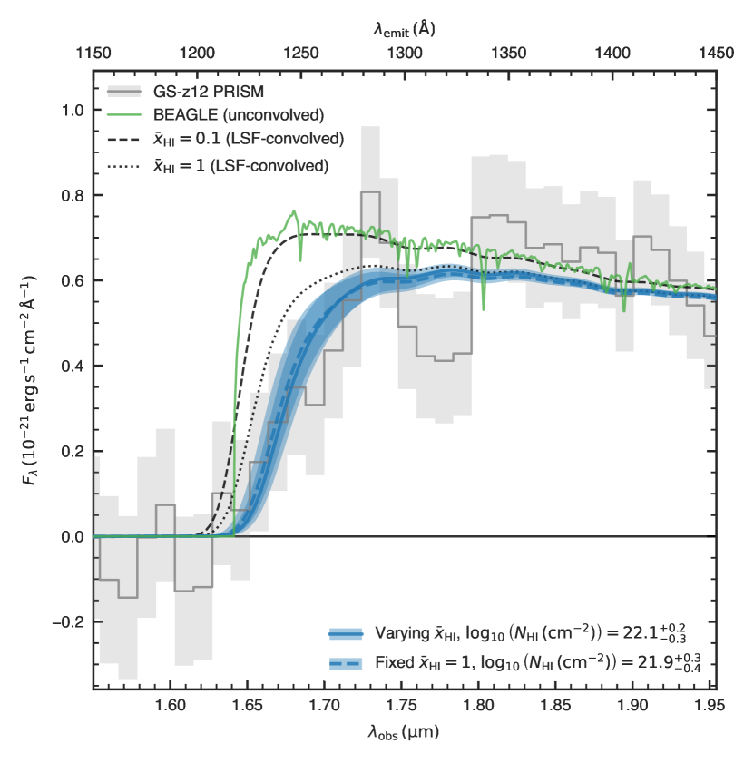
Figure 2: Fiducial (maximum-a-posteriori) spectrum (green) and data (grey) around the Ly transition. The dashed black line shows the effect of convolving the model spectrum with the prism LSF. The best-fit absorption profiles combining IGM and DLA absorption are shown by the blue lines and blue shading, assuming either a varying IGM neutral hydrogen fraction (solid line) or a fixed fraction $\bar{x}_{\text{{H}\,{\sc{i}}{}{}{}{}}}=1$ (dashed line). The IGM neutral hydrogen fraction is not well constrained, mainly because significant additional absorption is required to reconcile the profiles with the observed spectral break even with maximum IGM absorption ($\bar{x}_{\text{{H}\,{\sc{i}}{}{}{}{}}}=1$; see text for details).

Assuming that the dust attenuation through this neutral medium is the same as through the ISM of , i.e. $\tauv=0.05\pm 0.02$ (obtained as $0.4\cdot\beagletauv$, see § 3), we can obtain an order-of-magnitude estimate of the metallicity of the DLA gas as

$$Z_{\mathrm{DLA}}=Z_{\mathrm{MW}}\frac{\left(\tauv/N_{\text{{H}\,{\sc{i}}{}{}{}{}}}\right)_{\mathrm{DLA}}}{\left(\tauv/N_{\text{{H}\,{\sc{i}}{}{}{}{}}}\right)_{\mathrm{MW}}}\cdot\frac{\xi_{\mathrm{d,MW}}}{\xi_{\mathrm{d,DLA}}}.$$ (1)

The gas-to-extinction ratio we observe in the Milky Way is $\NHI/\tauv=(1.92\pm 0.02)\times 10^{21}\,\percm{-2}$ (e.g., Zhu et al., 2017), and the dust-to-metal ratio is $\xi_{\mathrm{d,MW}}=0.45$ (e.g., Konstantopoulou et al., 2023). The metallicity of the ISM in the solar neighbourhood is 0.2 dex lower than solar (Arellano-Córdova et al., 2021), therefore, we assume $Z_{\mathrm{MW}}=0.6$ solar. At low metallicity and at high gas fractions (as appropriate for ) is lower (De Cia et al., 2016; De Vis et al., 2019). Assuming a metallicity in the range 0.03–0.1 solar, the typical measured in high-redshift absorbers is $0.24\pm 0.11$ (e.g., Konstantopoulou et al., 2023). These values are on average half the Milky Way value. The above formula then gives us a DLA metallicity of 0.004–0.02 solar ($\logoh=6.3\text{--}7.0\leavevmode\nobreak\ \dex$), much lower than the estimate from § 3. We note that the large uncertainties in our assumptions are compounded by systematics in the spectral modelling with . For instance, using a 5-pixel extraction window (instead of the default 3-pixel) increases by approximately a factor 2. In addition, the optical depth estimated with relies on an ‘attenuation’ law (including absorption and scattering into and out of the line of sight caused by local and global geometric effects), while the column density from the DLA-like fit assumes a pure foreground ‘extinction’ curve (including absorption and scattering only out of the line of sight). Adopting an extinction rather than an attenuation curve in would provide lower – which would lower the metallicity estimate. Therefore, in the following, we treat our mean metallicity estimate of 6.6 dex as an upper limit.

Assuming all this gas is from the galaxy’s ISM – and that the DLA comes mostly from within one – we can estimate the mass of atomic gas as $\mgas=2\leavevmode\nobreak\ (1.34\leavevmode\nobreak\ m_{\mathrm{H}}\leavevmode\nobreak\ \NHI)\leavevmode\nobreak\ \text{\textpi}q\re^{2}$, giving $\log\,(\mgas/\MSun)=7.0\pm 0.25$ (where $m_{\mathrm{H}}$ is the mass of the hydrogen atom, the factor 1.34 accounts for the helium fraction, the additional factor of 2 is a geometric factor assuming equal column density on the far side of the galaxy, and $q$ is the axis ratio of the galaxy; we used the morphological parameters from Table 2). This gas mass is 10–50 per cent of the stellar mass inferred by . However, this is only the mass of atomic hydrogen and does not take into account the fraction of molecular (or ionised) hydrogen, hence it should be considered a lower limit. Such a gas fraction (or even higher given that it is a lower boundary) is consistent with many other galaxies at high redshift (Tacconi et al., 2020).

The corresponding lower limit on the gas surface density is 150  pc^-2 – at the boundary between normal star-forming regions and starbursts galaxies in the local Universe (e.g., Kennicutt & Evans, 2012). At these densities, most cold gas in the local Universe is expected to be in the molecular phase.

The SFR density inferred combining and the size measurement is of order $100\leavevmode\nobreak\ \MSun\leavevmode\nobreak\ \peryr\leavevmode\nobreak\ \mathrm{kpc}^{-2}$. Together with the gas surface density estimated above, this would place this galaxy well above the Schmidt–Kennicutt (S-K) relation, even for starburst galaxies. However, it could be consistent with the S-K relation considering that the surface density inferred above is a lower limit, and implying, once again, that a significant fraction of the gas is in molecular form.

5 Source of photo-ionisation and chemical abundances

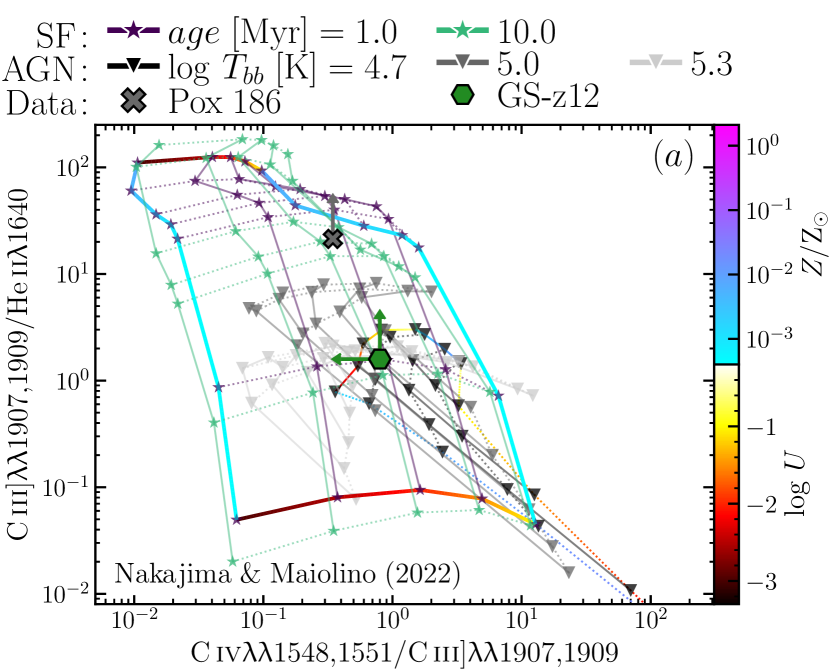
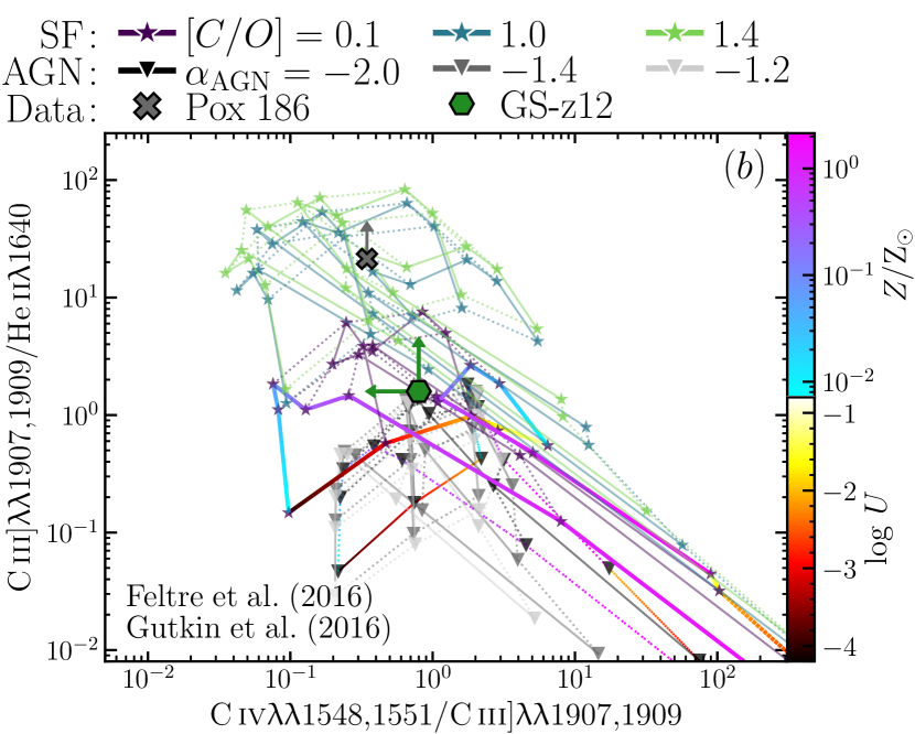
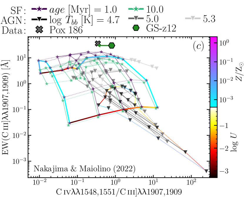
Figure 3: Panels 3–3; photo-ionisation diagnostics for star-formation (stars) and AGN (triangles), compared to (hexagon) and to the local analogue cross, Kumari et al., 2023. Panel 3; photo-ionisation diagnostic with EW(C iii]). The grids are from (panels 3 and 3), and from and (panel 3). All upper and lower limits are given at 3 .

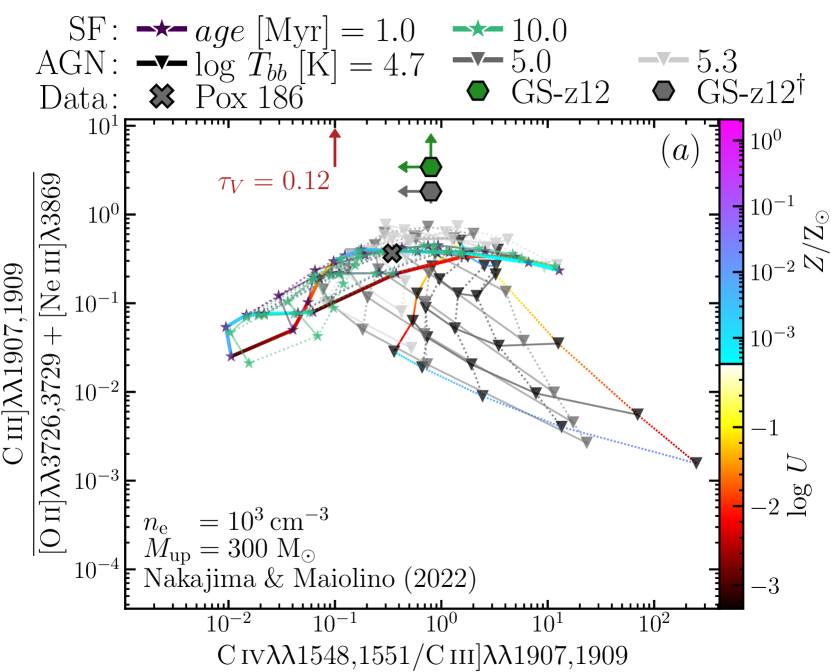
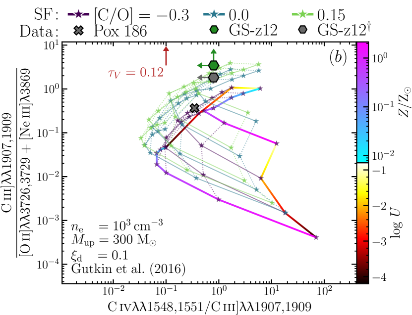
Figure 4: Panel 4; our upper limits on (hexagon), compared to photo-ionisation models powered by star formation (SF; stars) and AGN (triangles; , ), illustrating that lies well outside the range of grids with solar and subsolar C/O used by . Panel 4; star-forming models of , with varying C/O abundance between 0.5 and 1.4 solar. Combining the detection of C iii]1909 with stringent upper limits on [O ii]3726,3729 and [Ne iii]3869, the models constrain the abundance to super-solar values, i.e. much higher values than what is observed in galaxies at $z=9$ (see Fig. 5) and in the local analogue (Kumari et al., 2023). Alternatively, assuming both [O ii] and [Ne iii] to be detected, we obtain the grey hexagon marked with a ^†, which points to a solar  – still high for high-redshift galaxies. The red upward arrow marks the magnitude of the dust reddening correction, which we conservatively do not apply. We colour code only the external lines in the grids, and only for one of the SF and AGN grids; note the different range of the grid parameters.

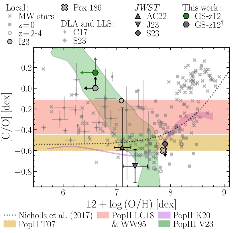
Figure 5: Compilation of chemical abundance patterns from both local stars and galaxies (see text for references) and from metal-poor galaxies at $z=2\text{--}9$, compared to the yields of PopII and PopIII supernovae. stands out as a metal-poor system with high C/O abundance, and is therefore closer to DLA systems Cooke et al., 2017, C17; Saccardi et al., 2023, S23 than to other high-redshift galaxies recently observed by Arellano-Córdova et al., 2022, AC22; Jones et al., 2023, J23; Stiavelli et al., 2023, S23. The dotted line is the chemical enrichment pattern from Nicholls et al. (2017); the golden horizontal hatched band is the yield of PopII supernovae from Tominaga et al. (2007). The purple region is the PopII abundance pattern from Kobayashi et al. (2020). The red horizontal band is the combined yield of metal-poor Type-II supernovae from Woosley & Weaver (1995) and Limongi & Chieffi (2018). The green region is the yield of PopIII supernovae Heger & Woosley, 2010, adapted from Vanni et al., 2023. We adopt the solar abundance ratio $\log(\mathrm{C/O})=-0.26$ (Asplund et al., 2009).

To identify the source of photo-ionisation in , we rely on models from the literature. The high value of EW(C iii]) rules out pristine sources like Population III stars and direct-collapse black holes Nakajima & Maiolino, 2022; hereafter: . We therefore focus on star-formation and AGN photo-ionisation, using models from , Feltre et al. (2016, hereafter: ) and Gutkin et al. (2016, hereafter: ). In the following, the grids of star-forming models are marked with stars, and those of AGNs are marked by triangles. For the star-forming models of , we fix the upper-mass cut-off of the IMF to 300 ; for their AGN models, we fix the shape of the ionising continuum to have a slope $\alpha_{\mathrm{AGN}}=-2$. In both cases, the density is $\nelec=10^{3}\,\percm{-3}$. For the star-forming models of , we fix the upper-mass cut-off of the IMF to 300 , the dust-to-metal mass ratio $\xid=0.1$, the maximum stellar age to 100 Myr, and the density to $\nelec=10^{2}\,\percm{-3}$. For the AGN models of , we fix both $\xid=0.1$ and $\nelec=10^{3}\,\percm{-3}$. We colour-code the external envelope of some of the grids by their metallicity $Z$ and ionisation parameter $\log\,U$. Each of these models presents unique advantages: extend to very low metallicity, and also provide EWs; the other two models provide independently varying C/O abundances.

In Fig. 3–3 the green hexagon shows the NIRSpec 3-upper limits in the UV diagnostic diagram using C iv, C iii] and He ii1640 (hereafter: He ii; ; , ). We also report the position of the local analogue as a cross; while the stringent upper limits on place it confidently in the star-forming region of the diagram, is in the upper envelope of the AGN models (panel 3). Given the trend of increasing C iii]/He ii with decreasing metallicity, we expect that extending the metallicity range of the grid to lower values would also allow these models to overlap with . In Fig. 3, we show EW(C iii]) vs C iv/C iii] for the models; both and the local analogue cannot be explained by either star-formation or AGN photo-ionisation. However, we note that the models assume the C/O enrichment scaling derived from the local Universe (Dopita et al., 2006); therefore, at the lowest metallicities relevant to this work, their C/O abundance is significantly sub-solar, and actually closer to the pure yield of Type-II supernovae.

In Fig. 4 we explore the C/O abundance ratio using the upper limits on both [O ii] and [Ne iii]– leveraging the fact that both O and Ne are elements released by Type-II supernovae. The standard enrichment pattern at the root of the models of cannot explain the observed lower limit (panel 4). The star-forming models of , in contrast, allow C/O to vary independently of the total metallicity. To explain the observations of (green hexagon), we thus require a super-solar $\CO>0.15\leavevmode\nobreak\ \dex$ i.e., higher than the highest value explored by the models. Even assuming [O ii] and [Ne iii] detections, we would still obtain $\CO\approx 0\leavevmode\nobreak\ \dex$ (grey hexagon). This abundance pattern, with higher-than-solar C/O, would also alleviate the tension with the EW measurements (Fig. 3). Changing the upper-mass cut of the IMF from 300 to 100 and the maximum stellar age from 100 to 10 Myr does not change our conclusions. Increasing the dust-to-metal mass fraction from 0.1 to 0.3 would instead make our conclusions even stronger, by lowering the predicted C iii]/([O ii] +[Ne iii]) ratio (because C has a higher depletion than Ne and O).

Fig. 5 shows the abundance ratio C/O vs , including Milky Way stars (grey crosses; Gustafsson et al., 1999; Akerman et al., 2004; Fabbian et al., 2009; Nissen et al., 2014), galaxies ranging from the local Universe (squares, labelled $z=0$; Berg et al., 2016; Peña-Guerrero et al., 2017; Senchyna et al., 2017; Berg et al., 2019) up to Cosmic Noon (empty circles, labelled $z=2$-4; Erb et al., 2010; Christensen et al., 2012; Bayliss et al., 2014; James et al., 2014; Stark et al., 2014; Berg et al., 2018; Mainali et al., 2020; Matthee et al., 2021; Iani et al., 2023), and DLAs (Cooke et al., 2017; Saccardi et al., 2023). We also show the abundances (and upper limits) from four high-redshift galaxies at $z=6\text{--}9$ measured by (Arellano-Córdova et al., 2022; Jones et al., 2023; Stiavelli et al., 2023). These galaxies tend to display a low [C/O]$\approx-0.6\,\dex$, very close to or even lower than the yield of metal-poor Type-II supernovae golden horizontal band, Tominaga et al., 2007; red horizontal band, Woosley & Weaver, 1995 and Limongi & Chieffi, 2018; purple region, Kobayashi et al., 2020. Indeed, these galaxies follow qualitatively the enrichment sequence from Nicholls et al. (2017), which is interpreted as a mixing sequence between the pure Type-II yields of young, low-metallicity systems, and the later contribution of stars on the asymptotic giant branch (AGB), which have longer enrichment timescales than Type-II supernovae (e.g., Salaris et al., 2014).

, instead, appears as an outlier relative to other galaxies, but it is consistent with some high-z DLAs. Specifically, its metallicity has an upper limit of 6.6 , as estimated from combining and (§§ 3 and 4). The C/O abundance is a lower limit, based on the lower limit on the C iii]/([O ii] +[Ne iii]) line ratio (§ 5). These values place clearly outside the rising enrichment sequence of local and lower redshift galaxies, and closer to the decreasing branch occupied by DLAs and extremely metal-poor stars in the Milky Way halo.

When compared with the models discussed above, the chemical enrichment pattern of is inconsistent with pure Type-II supernovae yields. Yet, its C/O and low metallicity suggest an enrichment history more similar to DLAs (small grey triangles). The yields of PopIII supernovae from Vanni et al. (2023, green band) give a sequence of super-solar C/O that may explain the lower limit of . Crucially, these models produce super-solar C/O via low-energy PopIII supernovae ($E<2\times 10^{51}$ erg; Vanni et al., 2023).

6 Summary, discussion and outlook

NIRSpec MSA observations from the combined programmes PID 1210 and 3215 enabled us to investigate the detailed physical properties of , a galaxy at $z>12$, near Cosmic Dawn. We report the detection of C iii] at $z=\zspec$. This is the most distant nebular-line detection to date, and the most distant evidence of chemical enrichment.

A full spectral modelling with the tool confirms the earlier results from ; has a stellar mass $\mstar=4\times 10^{7}\leavevmode\nobreak\ \MSun$ and a mass-doubling time of 40 Myr. The fit indicates a moderate dust attenuation optical depth, $\tauv=0.12$, and a sub-solar metallicity of =7.9 , mostly constrained by the emission lines.

The redshift obtained through the C iii] line implies that the Ly drop has a prominent damping wing. This cannot be associated only with IGM absorption, but can be modelled with absorption by the ISM of the galaxy or its CGM (i.e., a local DLA). Specifically, thanks to the accurate redshift obtained from the nebular emission lines, we can reliably model the damping wing profile and infer a high column density of $\NHI\approx 10^{22}\leavevmode\nobreak\ \percm{-2}$. The inferred gas fraction (/) is about 0.1–0.5, consistent with what one would expect at these high redshifts (Carilli & Walter, 2013; Tacconi et al., 2020). We note, however, that the uncertainties on the conversion from to and on the stellar mass-to-light ratio (due for instance to a top-heavy IMF, e.g., Rusakov et al., 2023) can be large. Converting this gas mass and the SFR into surface densities, we obtain values 150  pc^-2 and 100   kpc^-2, respectively. This combination is one to two orders of magnitude higher than the predictions from the local Schmidt–Kennicutt relation (Kennicutt & Evans, 2012), suggesting that we are missing a substantial fraction of the gas, very likely in the molecular form, or that our SFRs are significantly overestimated.

The gas metallicity we infer from is also quite uncertain, given the unwarranted assumption that estimated from the stellar continuum also applies to the Ly absorber. This is compounded by the large uncertainties on the dust-to-metal ratio () at these early epochs. With an average estimate of $\xid=0.24$ (Konstantopoulou et al., 2023) we obtain a sub-solar metallicity of about 0.004–0.02 solar, smaller than the value inferred from .

The high EW(C iii]) is reminiscent of lower-redshift AGN (Le Fèvre et al., 2019), but the lack of C iv emission seems at odds with this scenario. Unfortunately, and in spite of a 50 h-long integration, the upper limits on C iv and He ii are unable to definitely rule out the presence of an AGN (Fig. 3–3; we set a threshold of 3-for the non detections, or 99.9 per cent confidence). A local galaxy with properties analogue to , i.e. with a high-EW C iii] emission, is the low-mass, metal-poor star-forming dwarf galaxy (Kumari et al., 2023). and have similar size of $\approx$100 pc, yet, they have different masses (by two orders of magnitude) and markedly different C/O abundances.

The detection of C iii]– and its high EW – rules out scenarios of pristine stellar populations (PopIII) or black holes direct-collapse black holes; . The high-EW value of $30\pm 7\leavevmode\nobreak\ \AA$ cannot be explained with the sub-solar C/O ratio of the models. Kumari et al. (2023) have found similar difficulties in explaining the emission-line properties of (grey cross in Fig. 3) – perhaps exacerbated by the sub-solar C/O measured in their dwarf galaxy.

The long integration time of these observations provides stringent upper limits on both [O ii] and [Ne iii], which we use to study the C/O ratio (Fig. 4). The inability of subsolar- C/O models to explain the observed lower limits on C iii]/([O ii] +[Ne iii]) suggests that the bulk of the gas in has super-solar C/O abundance. While the prism data indicate a tentative detection of [O ii] and [Ne iii], we do not consider these detections to be robust (see § 2.3). Nevertheless, if we replace the 3-upper limits in C iii]/([O ii] +[Ne iii]) with detections, the line ratio decreases from 3.4 down to 1.8, which would still require a solar C/O (Fig. 4). In addition, throughout our analysis we do not apply any dust correction, but we note that any correction would increase the C iii]/([O ii] +[Ne iii]) ratio and the C/O abundance, making our result even stronger.

We note that the lower limit on C/O that we obtain is based on photo-ionisation models, which themselves rely on several assumptions about the shape of the ionising sources and the gas chemical abundance patterns. However, taking our results at face value, we find valuable implications on the chemical evolution history of this early galaxy.

In Fig. 5, we showed the location of in the O/H vs C/O enrichment diagram. The high C/O and low metallicity of this galaxy are inconsistent with the yields of Type-II supernovae ([C/O]$\lesssim-0.15$ dex), and much higher than what found by in galaxies at $z=6\text{--}9$ (Arellano-Córdova et al., 2022; Jones et al., 2023; Stiavelli et al., 2023).

Stars with extremely high C abundance have been found in the Milky Way, and these have some of the lowest measured Fe/H abundances (Aoki et al., 2006). While for these old galactic stars other enrichment channels are possible (dredge up or interactions with asymptotic-giant-branch companions, AGB), these scenarios seem inadequate for the case of , as dredge up is most appropriate for evolved low-mass stars (as is the case for Aoki et al., 2006). Specifically, AGB stars would need to dominate the chemical enrichment history of , but at $z=\zspec$ only stars more massive than $3\leavevmode\nobreak\ \MSun$ have had sufficient time to reach this phase, implying that the chemical enrichment history is still dominated by core-collapse supernovae. Besides, most metal-poor, C-rich stars in the Milky Way have solar or even sub-solar C/O abundance with Aoki et al., 2006 representing the exception, with $\CO>0.26$.

A possible explanation for this anomalously high value is that the stars in carry the signature of chemical enrichment due to massive, metal-poor stars, whose yields can be significantly different than those of PopII Type-II supernovae. In particular, chemical enrichment from PopIII can potentially explain the observed C/O in (Heger & Woosley, 2010; Limongi & Chieffi, 2018), especially when including low-energy supernova explosions (Vanni et al., 2023). These explosions leave remnants with a higher fraction of the O-rich shell locked in them, with respect to the C-rich shell, thereby increasing the C/O yield of the ejecta to solar or even super-solar values. An alternative explanation is represented by peculiar star-formation histories, such as those invoked to explain the abundance patterns in GN-z11 (Kobayashi & Ferrara, 2023). Such peculiar SFHs would, however, also produce a strong nitrogen abundance, which is inconsistent with the observations of .

This detection of the most distant metal transition, which has provided such precious information about the earliest phases of the chemical enrichment, has required a very long exposure (65 h, although mostly as a parallel observation). This is due to the extreme faintness of such distant galaxies. However, in the future, large-area surveys and gravitational lenses may help identify more high-redshift galaxies that are sufficiently bright for deep spectroscopic follow up with shorter exposures.

Appendix A In-depth analysis of the data

In §§ 2.2 and 2.3 we summarised our considerations on the reliability of the emission lines detections. The goal of this section is to provide more information on the data, and on the reliability of the various emission-line detections – particularly in the low-S/N regime. To do so, we take advantage of 162 individual integrations for , each with 1,400.5 s duration. We show the S/N as a function of wavelength for each of these detections in Fig. 6; the y-axis values from 0 to 113 correspond to the 114 integrations five visits from PID 3215; the remaining 48 integrations are from two visits in PID 1210. We saturate the colour limits between S/N 0 and 2, to highlight a faint vertical line at 2.57 , which we interpret as C iii]. No other emission lines are clearly visible in this representation. In particular, we see no evidence for [O ii] or [Ne iii]; even though these two lines have lover S/N than C iii] (which should make them harder too see), they occupy a region of the spectrum with lower continuum flux than C iii] (which would enhance the contrast with neighbouring pixels). The 162 individual spectra are also shown in panel 6; while this figure is dominated by noise, the C iii] line is also visible here. Panel 6 shows the 16^th, 50^th and 84^th percentiles of the data in panel 6. The vertical lines mark the locations of O iii], C iii], [O ii] and [Ne iii]. In this figure, C iii] and [O ii] are clearly seen, while O iii] seems absent and so does [Ne iii]. This line in particular has an ugly spectral profile, which further validates our decision to treat it as a tentative detection only.

Panel 6 shows a comparison between the noise of our co-added data, derived from the data reduction pipeline (black) and the dispersion of the 162 exposures (grey), estimated as the 84^th-16^th inter-percentile range divided by $2\cdot\sqrt{162}$. The latter estimate is 25–30 per cent smaller than the former, but it does not take into account correlated noise due to spectral resampling on the NIRSpec detector. In contrast, the data reduction pipeline implements an effective correction to the noise (Dorner et al., 2016), giving a more conservative estimate. Using the grey curve as noise vector, the C iii] S/N would increase to 7–7.5.

Finally, in panel 6 we show the 1-d spectra from PID 1210 (cyan) and 3215 (sand), including zoom-in windows around the Ly drop, O iii]–C iii] and [O ii]-[Ne iii] (panels 6–6). This comparison in particular shows that O iii] seems absent in 3215, but a single high pixel in 1210 may be driving its 2.3 tentative detection; C iii], in contrast, appears to have similar profiles at the same location in both 1210 and 3215 (panel 6). [O ii] appears both in 1210 and 3215, but, as we have mentioned, its wavelength is different between the two observations. An issue due to the wavelength solution seems unlikely, because the galaxy is well centred in the MSA shutter, and because the shift in spectral pixels due to intra-shutter position is negligible at these red wavelengths. If any problem in the wavelength calibration was present, it could potentially explain the moderate mismatch in redshift between C iii] and [O ii]–[Ne iii]. [Ne iii] confirms its dubious nature, especially in 1210, where it shows a narrow profile that does not resemble a true emission line.

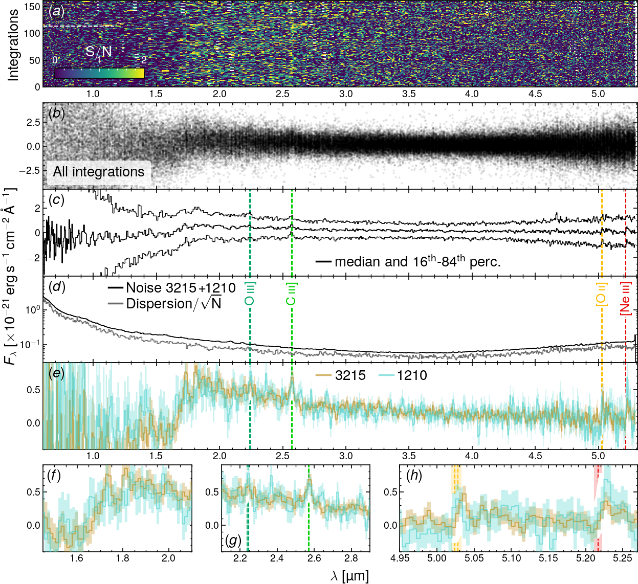
Figure 6: Summary of the prism observations. Panel 6; S/N of each of the 162 individual integrations. The horizontal dashed line separates the bottom 114 rows with the 3215 integrations from the 1210 integrations above. Panel 6; spectrum of each of the individual integrations. A feature at the location of C iii] is clearly seen. Panel 6; median and 16^th–84^th percentile of panel 6, showing again the presence of C iii], and the possible presence of [O ii]. Panel 6; comparison between the noise estimated by the data reduction pipeline (black) with the noise estimated from the dispersion of the integrations (grey, calculated under a Gaussian-noise assumption). Panels 6–6; comparison between 3215 (sand) and 1210 (cyan), showing that C iii] is seen in both programmes; in contrast, O iii] is not seen in 3215 (the deepest of the two surveys); an emission line close to the position of [O ii] is seen in both surveys, but at different wavelengths; [Ne iii] is seen in 3215, but has an unconvincing line profile in 1210.

In Fig. 7 we show the jackknife spectra obtained by stacking all the individual integrations, but excluding the integrations from a single visit at a time. This procedure highlights whether the emission lines we see in the data arise from a detector feature, which may be in common between all the integrations from the same visit.

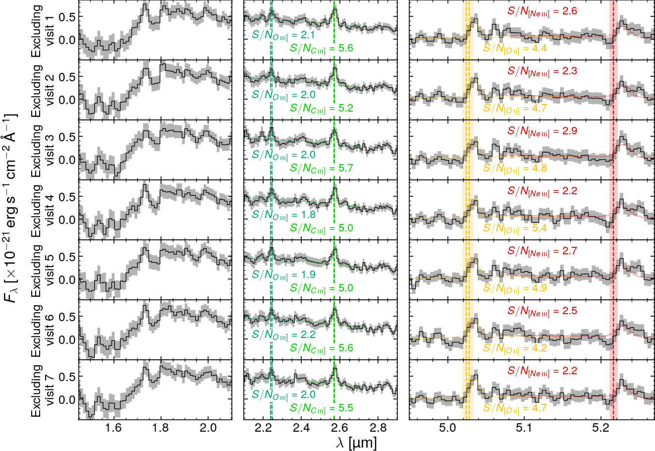
Figure 7: Jackknife combination of the prism data; each row is obtained by excluding all the integrations from one of the seven visits and combining the rest. The first two rows exclude the first and second visit from PID 1210; the bottom five rows each exclude one of the visits from PID 3215. The vertical dashed lines and shaded regions are the same as in Figs. 1 and 6. The labels report the S/N of each line. C iii] appears well detected in all combinations, meaning that this line is unlikely to arise from detector artefacts (which may be present in all the integrations from the same visit). The different S/N compared to the fiducial fits are due to the different model adopted here (see text for more details).

The stacked spectra are obtained by applying an iterative 3-clipping algorithm in each wavelength pixel, and by applying inverse- variance weighting. We fit a single Gaussian with a local linear background around each of O iii], C iii], [O ii] and [Ne iii]. Overall, we find that C iii] is confirmed at 5-significance, and does not appear to be driven by any single visit. The uncertainties about O iii] and [Ne iii] are larger than in the fiducial fit, reflecting the increased number of free parameters used here.

We perform the same test in the left column of Fig 8, but only for PID 3215, because in PID 1210 the G395M exposure time is much shorter than in PID 3215 (only 10 per cent of the total time, Table 1). We find no evidence of strong artefacts in any of the visits. As a recovery test, we add a single Gaussian emission line with flux equal to the [O ii] flux measured from the prism, dispersion equal to one pixel, and centred at the expected location of the [O ii] doublet (vertical dashed lines). The second and third columns in Fig 8 show a comparison between the data without and with the artificial line injection. This is the best-case scenario of a single, spectrally unresolved emission line; any additional broadening (e.g., due to the doblet nature of [O ii]) would make the following estimates more conservative. We estimate the line sensitivity by integrating the variance spectrum from the pipeline over two spectral pixels; based on the (conservative) pipeline uncertainties, we should be able to measure this artificial line with S/N=3. This would suggest that at least one of [O ii] or [Ne iii] should be seen in the grating data. However, the injection test shows that the effective S/N of the artificial line is likely lower than 3, and that we would not be able to detect [O ii] or [Ne iii].

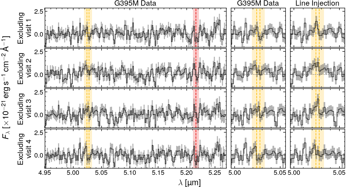
Figure 8: Jackknife combination of the G395M grating data; each row is obtained by excluding all the integrations from one of the four visits in PID 3215 and combining the rest Table 1). The first column displays the spectral region of interest, the second column is a zoom-in on the region of [O ii], the third column is the same as the second, but we added a Gaussian emission line with total flux equal to the [O ii] flux measured in the prism. The vertical dashed lines and shaded regions are the same as in Figs. 1 and 6 and highlight the expected wavelengths of [O ii] (orange) and [Ne iii] (red). Given the noise of these observations, this line is unlikely to arise from detector artefacts (which may be present in all the integrations from the same visit). The different S/N compared to the fiducial fits are due to the different model adopted here (see text for more details).

References

- Akerman et al. (2004) Akerman, C. J., Carigi, L., Nissen, P. E., Pettini, M., & Asplund, M. 2004, A&A, 414, 931
- Aoki et al. (2006) Aoki, W., Frebel, A., Christlieb, N., et al. 2006, ApJ, 639, 897
- Arellano-Córdova et al. (2022) Arellano-Córdova, K. Z., Berg, D. A., Chisholm, J., et al. 2022, ApJ, 940, L23
- Arellano-Córdova et al. (2021) Arellano-Córdova, K. Z., Esteban, C., García-Rojas, J., & Méndez-Delgado, J. E. 2021, MNRAS, 502, 225
- Arrabal Haro et al. (2023) Arrabal Haro, P., Dickinson, M., Finkelstein, S. L., et al. 2023, ApJ, 951, L22
- Asplund et al. (2009) Asplund, M., Grevesse, N., Sauval, A. J., & Scott, P. 2009, ARA&A, 47, 481
- Astropy Collaboration et al. (2013) Astropy Collaboration, Robitaille, T. P., Tollerud, E. J., et al. 2013, A&A, 558, A33
- Baker et al. (2023) Baker, W. M., Tacchella, S., Johnson, B. D., et al. 2023, arXiv e-prints, arXiv:2306.02472
- Bayliss et al. (2014) Bayliss, M. B., Rigby, J. R., Sharon, K., et al. 2014, ApJ, 790, 144
- Berg et al. (2018) Berg, D. A., Erb, D. K., Auger, M. W., Pettini, M., & Brammer, G. B. 2018, ApJ, 859, 164
- Berg et al. (2019) Berg, D. A., Erb, D. K., Henry, R. B. C., Skillman, E. D., & McQuinn, K. B. W. 2019, ApJ, 874, 93
- Berg et al. (2016) Berg, D. A., Skillman, E. D., Henry, R. B. C., Erb, D. K., & Carigi, L. 2016, ApJ, 827, 126
- Bunker et al. (2023a) Bunker, A. J., Cameron, A. J., Curtis-Lake, E., et al. 2023a, arXiv e-prints, arXiv:2306.02467
- Bunker et al. (2023b) Bunker, A. J., Saxena, A., Cameron, A. J., et al. 2023b, A&A, 677, A88
- Cameron et al. (2023a) Cameron, A. J., Katz, H., Rey, M. P., & Saxena, A. 2023a, MNRAS, 523, 3516
- Cameron et al. (2023b) Cameron, A. J., Saxena, A., Bunker, A. J., et al. 2023b, A&A, 677, A115
- Cappellari et al. (2013) Cappellari, M., Scott, N., Alatalo, K., et al. 2013, MNRAS, 432, 1709
- Carilli & Walter (2013) Carilli, C. L. & Walter, F. 2013, ARA&A, 51, 105
- Carniani et al. (2023) Carniani, S., Venturi, G., Parlanti, E., et al. 2023, arXiv e-prints, arXiv:2306.11801
- Chabrier (2003) Chabrier, G. 2003, PASP, 115, 763
- Charlot & Fall (2000) Charlot, S. & Fall, S. M. 2000, ApJ, 539, 718
- Chevallard & Charlot (2016) Chevallard, J. & Charlot, S. 2016, MNRAS, 462, 1415
- Christensen et al. (2012) Christensen, L., Laursen, P., Richard, J., et al. 2012, MNRAS, 427, 1973
- Cooke et al. (2017) Cooke, R. J., Pettini, M., & Steidel, C. C. 2017, MNRAS, 467, 802
- Curti et al. (2023a) Curti, M., D’Eugenio, F., Carniani, S., et al. 2023a, MNRAS, 518, 425
- Curti et al. (2023b) Curti, M., Maiolino, R., Curtis-Lake, E., et al. 2023b, arXiv e-prints, arXiv:2304.08516
- Curtis-Lake et al. (2023) Curtis-Lake, E., Carniani, S., Cameron, A., et al. 2023, Nature Astronomy, 7, 622
- De Cia et al. (2016) De Cia, A., Ledoux, C., Mattsson, L., et al. 2016, A&A, 596, A97
- de Graaff et al. (2023) de Graaff, A., Rix, H.-W., Carniani, S., et al. 2023, arXiv e-prints, arXiv:2308.09742
- De Vis et al. (2019) De Vis, P., Jones, A., Viaene, S., et al. 2019, A&A, 623, A5
- Dopita et al. (2006) Dopita, M. A., Fischera, J., Sutherland, R. S., et al. 2006, ApJS, 167, 177
- Dorner et al. (2016) Dorner, B., Giardino, G., Ferruit, P., et al. 2016, A&A, 592, A113
- Dressler et al. (2023) Dressler, A., Rieke, M., Eisenstein, D., et al. 2023, arXiv e-prints, arXiv:2306.02469
- Eisenstein et al. (2023a) Eisenstein, D. J., Johnson, B. D., Robertson, B., et al. 2023a, arXiv e-prints, arXiv:2310.12340
- Eisenstein et al. (2023b) Eisenstein, D. J., Willott, C., Alberts, S., et al. 2023b, arXiv e-prints, arXiv:2306.02465
- Endsley et al. (2023) Endsley, R., Stark, D. P., Whitler, L., et al. 2023, arXiv e-prints, arXiv:2306.05295
- Erb et al. (2010) Erb, D. K., Pettini, M., Shapley, A. E., et al. 2010, ApJ, 719, 1168
- Fabbian et al. (2009) Fabbian, D., Nissen, P. E., Asplund, M., Pettini, M., & Akerman, C. 2009, A&A, 500, 1143
- Feltre et al. (2016) Feltre, A., Charlot, S., & Gutkin, J. 2016, MNRAS, 456, 3354
- Foreman-Mackey et al. (2013) Foreman-Mackey, D., Hogg, D. W., Lang, D., & Goodman, J. 2013, PASP, 125, 306
- Frebel & Norris (2015) Frebel, A. & Norris, J. E. 2015, ARA&A, 53, 631
- Fumagalli et al. (2016) Fumagalli, M., O’Meara, J. M., & Prochaska, J. X. 2016, MNRAS, 455, 4100
- Gustafsson et al. (1999) Gustafsson, B., Karlsson, T., Olsson, E., Edvardsson, B., & Ryde, N. 1999, A&A, 342, 426
- Gutkin et al. (2016) Gutkin, J., Charlot, S., & Bruzual, G. 2016, MNRAS, 462, 1757
- Harris et al. (2020) Harris, C. R., Millman, K. J., van der Walt, S. J., et al. 2020, Nature, 585, 357
- Heger & Woosley (2010) Heger, A. & Woosley, S. E. 2010, ApJ, 724, 341
- Heintz et al. (2023) Heintz, K. E., Watson, D., Brammer, G., et al. 2023, arXiv e-prints, arXiv:2306.00647
- Hirano et al. (2014) Hirano, S., Hosokawa, T., Yoshida, N., et al. 2014, ApJ, 781, 60
- Hosokawa et al. (2011) Hosokawa, T., Omukai, K., Yoshida, N., & Yorke, H. W. 2011, Science, 334, 1250
- Hsiao et al. (2023) Hsiao, T. Y.-Y., Abdurro’uf, Coe, D., et al. 2023, arXiv e-prints, arXiv:2305.03042
- Hunter (2007) Hunter, J. D. 2007, Computing in Science and Engineering, 9, 90
- Iani et al. (2023) Iani, E., Zanella, A., Vernet, J., et al. 2023, MNRAS, 518, 5018
- James et al. (2014) James, B. L., Pettini, M., Christensen, L., et al. 2014, MNRAS, 440, 1794
- Jones et al. (2001) Jones, E., Oliphant, T., Peterson, P., et al. 2001, SciPy: Open source scientific tools for Python, [Online; accessed ¡today¿]
- Jones et al. (2023) Jones, T., Sanders, R., Chen, Y., et al. 2023, ApJ, 951, L17
- Kennicutt & Evans (2012) Kennicutt, R. C. & Evans, N. J. 2012, ARA&A, 50, 531
- Kobayashi & Ferrara (2023) Kobayashi, C. & Ferrara, A. 2023, arXiv e-prints, arXiv:2308.15583
- Kobayashi et al. (2020) Kobayashi, C., Karakas, A. I., & Lugaro, M. 2020, ApJ, 900, 179
- Konstantopoulou et al. (2023) Konstantopoulou, C., De Cia, A., Ledoux, C., et al. 2023, arXiv e-prints, arXiv:2310.07709
- Kumari et al. (2023) Kumari, N., Smit, R., Leitherer, C., et al. 2023, arXiv e-prints, arXiv:2307.00059
- Kunth et al. (1981) Kunth, D., Sargent, W. L. W., & Kowal, C. 1981, A&AS, 44, 229
- Le Fèvre et al. (2019) Le Fèvre, O., Lemaux, B. C., Nakajima, K., et al. 2019, A&A, 625, A51
- Limongi & Chieffi (2018) Limongi, M. & Chieffi, A. 2018, ApJS, 237, 13
- Looser et al. (2023) Looser, T. J., D’Eugenio, F., Maiolino, R., et al. 2023, arXiv e-prints, arXiv:2306.02470
- Mainali et al. (2020) Mainali, R., Stark, D. P., Tang, M., et al. 2020, MNRAS, 494, 719
- Maiolino et al. (2023) Maiolino, R., Scholtz, J., Witstok, J., et al. 2023, arXiv e-prints, arXiv:2305.12492
- Matthee et al. (2021) Matthee, J., Sobral, D., Hayes, M., et al. 2021, MNRAS, 505, 1382
- Nakajima & Maiolino (2022) Nakajima, K. & Maiolino, R. 2022, MNRAS, 513, 5134
- Nakajima et al. (2023) Nakajima, K., Ouchi, M., Isobe, Y., et al. 2023, arXiv e-prints, arXiv:2301.12825
- Nicholls et al. (2017) Nicholls, D. C., Sutherland, R. S., Dopita, M. A., Kewley, L. J., & Groves, B. A. 2017, MNRAS, 466, 4403
- Nissen et al. (2014) Nissen, P. E., Chen, Y. Q., Carigi, L., Schuster, W. J., & Zhao, G. 2014, A&A, 568, A25
- Oesch et al. (2016) Oesch, P. A., Brammer, G., van Dokkum, P. G., et al. 2016, ApJ, 819, 129
- Peña-Guerrero et al. (2017) Peña-Guerrero, M. A., Leitherer, C., de Mink, S., Wofford, A., & Kewley, L. 2017, ApJ, 847, 107
- Pedregosa et al. (2011) Pedregosa, F., Varoquaux, G., Gramfort, A., et al. 2011, Journal of Machine Learning Research, 12, 2825
- Pettini et al. (2008) Pettini, M., Zych, B. J., Steidel, C. C., & Chaffee, F. H. 2008, MNRAS, 385, 2011
- Planck Collaboration et al. (2020) Planck Collaboration, Aghanim, N., Akrami, Y., et al. 2020, A&A, 641, A6
- Reddy et al. (2023) Reddy, N. A., Topping, M. W., Sanders, R. L., Shapley, A. E., & Brammer, G. 2023, ApJ, 952, 167
- Rieke et al. (2023) Rieke, M., Robertson, B., Tacchella, S., et al. 2023, arXiv e-prints, arXiv:2306.02466
- Robertson (2022) Robertson, B. E. 2022, ARA&A, 60, 121
- Robertson et al. (2023) Robertson, B. E., Tacchella, S., Johnson, B. D., et al. 2023, Nature Astronomy, 7, 611
- Rusakov et al. (2023) Rusakov, V., Steinhardt, C. L., & Sneppen, A. 2023, ApJS, 268, 10
- Saccardi et al. (2023) Saccardi, A., Salvadori, S., D’Odorico, V., et al. 2023, ApJ, 948, 35
- Salaris et al. (2014) Salaris, M., Weiss, A., Cassarà, L. P., Piovan, L., & Chiosi, C. 2014, A&A, 565, A9
- Salvadori & Ferrara (2012) Salvadori, S. & Ferrara, A. 2012, MNRAS, 421, L29
- Schaerer et al. (2022) Schaerer, D., Marques-Chaves, R., Barrufet, L., et al. 2022, A&A, 665, L4
- Senchyna et al. (2023) Senchyna, P., Plat, A., Stark, D. P., & Rudie, G. C. 2023, arXiv e-prints, arXiv:2303.04179
- Senchyna et al. (2017) Senchyna, P., Stark, D. P., Vidal-García, A., et al. 2017, MNRAS, 472, 2608
- Stark et al. (2017) Stark, D. P., Ellis, R. S., Charlot, S., et al. 2017, MNRAS, 464, 469
- Stark et al. (2014) Stark, D. P., Richard, J., Siana, B., et al. 2014, MNRAS, 445, 3200
- Stiavelli et al. (2023) Stiavelli, M., Morishita, T., Chiaberge, M., et al. 2023, arXiv e-prints, arXiv:2308.14696
- Tacchella et al. (2023) Tacchella, S., Eisenstein, D. J., Hainline, K., et al. 2023, ApJ, 952, 74
- Tacconi et al. (2020) Tacconi, L. J., Genzel, R., & Sternberg, A. 2020, ARA&A, 58, 157
- Taylor (2005) Taylor, M. B. 2005, in Astronomical Society of the Pacific Conference Series, Vol. 347, Astronomical Data Analysis Software and Systems XIV, ed. P. Shopbell, M. Britton, & R. Ebert, 29
- Tominaga et al. (2007) Tominaga, N., Umeda, H., & Nomoto, K. 2007, ApJ, 660, 516
- van Rossum (1995) van Rossum, G. 1995, CWI Technical Report, CS-R9526
- Vanni et al. (2023) Vanni, I., Salvadori, S., Skúladóttir, Á., Rossi, M., & Koutsouridou, I. 2023, MNRAS, 526, 2620
- Witstok et al. (2023) Witstok, J., Smit, R., Saxena, A., et al. 2023, arXiv e-prints, arXiv:2306.04627
- Woosley & Weaver (1995) Woosley, S. E. & Weaver, T. A. 1995, ApJS, 101, 181
- Zhu et al. (2017) Zhu, H., Tian, W., Li, A., & Zhang, M. 2017, MNRAS, 471, 3494