Meridional Circulations of the Solar Magnetic Fields of Different Strength

1 Introduction

Solar plasma meridional circulation play a major role in the solar magnetic field dynamics. Meridional flows globally redistribute the solar plasma, heat, angular momentum, and magnetic fields in all layers from convective zone to the solar corona. Meridional flows are important in explaining the solar dynamo and differential rotation. They play a key role in the flux-transport dynamo models (Sheeley, 2005; Jiang et al., 2014; Hanasoge, 2022). Cycle variations of the meridional flow have been suggested to explain the changes in the amplitudes and lengths of the solar activity cycles (Charbonneau, 2020; Karak, 2023) and they also used for their prediction (Petrovay, 2020). Solar meridional circulation is considered to be an axisymmetric flow system, extending from the equator to the poles with $\approx$20 m s^-1 at the solar surface.

Various methods and traces are used to identify and measure meridional flows. Poleward flow has been detected using the Doppler method. Duvall and Jr. (1979) found a poleward flow of 20 m s^-1 approximately constant over the latitude range of 10^∘ – 50^∘. Studying giant velocity features about 15^∘ in latitude and 30 – 60^∘ in longitude with amplitudes around 40 m s^-1 on the solar surface, Howard (1979) have also found a meridional flow toward the poles of the order of 20 m s^-1. Using doppler velocities Hathaway (1996) determined an antisymmetric flow towards the poles of 20 m s^-1 about the equator in both hemispheres. For bright Ca+-mottles Schroeter and Woehl (1975) have found a systematic meridional motion of about 0.1 km s^-1 for latitudes around 10^∘. Topka et al. (1982) shown that polar filaments track the boundary latitudes of the unipolar magnetic regions and drift poleward with the regions at about 10 m s^-1. They noted that such a filament motion cannot be explained by diffusion alone, and that a poleward meridional flow carries magnetic flux of both polarities along with it.

Small magnetic elements are often used to determine the velocity of meridional flows (Rightmire-Upton, Hathaway, and Kosak, 2012). Komm, Howard, and Harvey (1993) found poleward meridional flow velocity of the order of 10 m s^-1 in each hemisphere for small magnetic elements using high-resolution magnetograms taken from 1978 to 1990 with the NSO Vacuum Telescope on Kitt Peak. The meridional flow was found to change during solar cycle. They showed that meridional flow increased in amplitude from the equator, reached a maximum of 13.2 m s^-1 at 39^∘, and decreased poleward. They found no significant hemispheric asymmetry and no equator ward migration. However, analyzing the Mt. Wilson magnetograms, Snodgrass and Dailey (1996) found that for latitudes near the equator the flow was towards the equator.

Meridional flows were found to change during solar cycles. Hathaway and Rightmire (2010) using SOHO data showed that the average flow speed of magnetic features was poleward at all latitudes up to 75^∘. They found that the flow was faster at sunspot cycle minimum than at maximum and it was changed from cycle to cycle. In Hathaway and Upton (2014) it was also found that the meridional flow speed of magnetic elements was fast at solar cycle minimum and slow at maximum. The meridional flow weakening on the poleward sides of the active region latitudes and it was slower at Solar Cycle 23. They proposed that an inflow towards the sunspot zones was superimposed on a more general poleward meridional flow. Imada et al. (2020) found that the average meridional flow in Solar Cycle 24 was faster than that in Solar Cycle 23.

Meridional motions have also been determined using coronal bright points from SOHO/EIT, Yohkoh/SXT, Hinode, and SDO/AIA data (Vršnak et al., 2003; Sudar et al., 2016). Vršnak et al. (2003) noted that a velocity pattern of bright point motions reflected the large-scale plasma flows. In a complex pattern of meridional motion, they found that the equator ward flows were dominated at low ($B<10^{\circ}$) and high ($B>40^{\circ}$) latitudes, and a poleward flow at mid-latitudes ($B\approx 10^{\circ}$ – 40^∘). Faster flow tracers had equator ward motion and the slower ones showed poleward motion.

Howard and Gilman (1986) studying the meridional motions of sunspots and sunspot groups found a midlatitude northward flow with a few hundredths of a degree per day in each hemisphere. For sunspot groups, a generally poleward motions at higher latitudes was determined. Sudar et al. (2014) considered the location measurements of sunspot groups covering 1878 – 2011. They found that the meridional motion of sunspot groups is towards the centre of activity from all latitudes and in all solar cycle phases. The range of meridional velocities was found to be $\pm 1$0 m s^-1.

Helioseismology makes it possible to study meridional flows at different layers in the solar interior (Gizon, 2004). Chou and Dai (2001) studying the subsurface meridional flow as a function of latitude and depth from 1994 to 2000, have found that the velocity of meridional flow increased when solar activity decreased. A new meridional flow component at about 20^∘ appeared in each hemisphere as solar activity increased. At low latitudes, the new flow changed from poleward at solar minimum to equatorward at solar maximum. The velocity of the new component increases with depth. In Basu and Antia (2003), it was revealed that the meridional flows showed solar activity-related changes. The antisymmetric component of the meridional flow decreased in speed with activity. Basu and Antia (2010) have shown that meridional-flow speed increases with depth. For Solar Cycle 23, they found that solar meridional flows in the outer 2% of the solar radius was connected with a flow pattern drifting equator ward in parallel with the activity belts. The different flow components was found to have different time dependencies, and the dependence was different at different depths. Zhao et al. (2013) using the helioseismology observations from the SDO/HMI, found the poleward meridional flow of a speed of 15 m s^-1 from the photosphere to about 0.91 R_⊙ and an equator ward flow of a speed of 10 m s^-1 between 0.82 and 0.91 R_⊙. They also found that the meridional flow turned poleward again below 0.82 R_⊙.

From all of the above it follows that in various studies, different authors defined meridional flows of different directions and velocities. In some studies significant temporal variations in the meridional flows were found, though they were not always in complete agreement with each other. The purpose of this study is to determine time-latitude variations in meridional flows by analyzing the dynamics of various strength positive- and negative-polarity photospheric magnetic fields. Section 2 describes the data used. In Section 3, the time-latitude distributions of the large-scale solar magnetic fields of positive and negative polarity in Cycles 21 – 24 are investigated. The time-latitude distributions of positive- and negative-polarity photospheric magnetic fields using the data with high spatial resolution are analyzed in Section 4. Variations in the magnitudes of the photospheric magnetic fields of different strength are considered in Section 5. Mean latitudes and velocities of different type meridional circulations are studied in Section 6. The results are discussed in Section 7. The main conclusions are listed in Section 8.

2 Data

Synoptic magnetic field data from ground based WSO (Wilcox Solar Observatory, (Scherrer et al., 1977; Duvall et al., 1977; Hoeksema, Wilcox, and Scherrer, 1983), NSO KPVT (Kitt Peak Vacuum Telescope, Livingston et al. (1976a, b); Jones et al. (1992)) and SOLIS/VSM (Synoptic Optical Long-Term Investigations/Vector Stokes Magnetograph, Keller, Harvey, and Giampapa (2003)), and space based SOHO/MDI (Solar and Heliospheric Observatory/Michelson Doppler Imager, Scherrer et al. (1995)) and SDO/HMI (Solar Dynamics Observatory/Helioseismic and Magnetic Imager, Scherrer et al. (2012); Schou et al. (2012)) observatories were used. These observatories were chosen because they represent the most often used data that overlap the greatest time interval of observations. All synoptic maps were used in their original format without any interpolation or changes. Synoptic maps are maps of the magnetic field latitude-longitude distribution, created on the base of daily observations. Each synoptic map span a full Carrington Rotation (CR, 1 CR = 27.2753 days). The entire data set consists of 616 synoptic maps and covers CRs 1642 – 2258 (May 1976 – May 2022). Data on magnetic fields are given in a longitude versus sine-latitude grid.

WSO provides the longest homogeneous series of observational data of the low-resolution large-scale photospheric magnetic fields (Hoeksema and Scherrer, 1988) since 1976 without major updates of magnetograph. The WSO synoptic maps represent the radial component of the photospheric magnetic field, derived from observations of the line-of-sight field component by assuming the field to be approximately radial. WSO aperture size is 3 arc-min, which means approximately 33 pixels in longitude in the equator. WSO synoptic magnetic-field maps consist of $30$ data points in equal steps of sine latitude from $70^{\circ}$S to $70^{\circ}$N. Longitude is presented in $5^{\circ}$ intervals. To convert WSO measured data to units of Gauss, a factor of 1.85 is required (Riley et al., 2014). ”F-data” files, where missing data are interpolated, were applied. WSO coronal magnetic field synoptic maps calculated from large-scale photospheric fields with a potential field radial model with the source-surface location at 2.5 R_⊙ (Schatten, Wilcox, and Ness, 1969; Altschuler and Newkirk, 1969; Hoeksema, Wilcox, and Scherrer, 1983) were also used.

Observations from KPVT (from 1976 to 2003, CRs 1625 – 2007) and SOLIS (from 2003 to 2017, CRs 2007 – 2127) were used to study the high-resolution photospheric magnetic fields. At the KPVT, the pixel size of images was 1.0” from CR 1625 to CR 1853, when a 512-channel Babcock type instrument was used, and 1.14” after CR 1855, when a CCD spectromagnetograph was used. SOLIS’s resolution was 1.125” until 2010, and 1.0” after that. Every KPVT and SOLIS synoptic map consists of 360$\times$180 pixels of magnetic field strength values in Gauss. KPVT and SOLIS CR maps span 0^∘ – 360^∘ solar longitude and from $90^{\circ}$S to $90^{\circ}$N sine solar latitude.

MDI instrument on board the SOHO spacecraft was operational from 1996 to 2011. There were data gaps in SOHO for June – October 1998 and January – February 1999. MDI synoptic map consists of 3600$\times$1080 pixels. MDI was succeeded by the HMI in 2010, with a short overlapping period. HMI provides magnetic field data with much higher spatial and temporal resolutions and better quality. The HMI synoptic maps have a size of 3600$\times$1440 pixels.

Synoptic data presented by WSO, KPVT, SOLIS, MDI, and HMI are different (Virtanen and Mursula, 2016, 2017, 2019). The observatories use different instruments, observation methods, data processing methods, different spectral lines, and different technic used for synoptic maps construction. Their data have different spatial and spectral resolutions. The instrumentation used at ground-based observatories changed during the period concerned. The method of polar magnetic field interpolation in synoptic maps used in different observatories also cause differences between the data sets. Therefore the values of magnetic field strength from different observatories differ significantly. For comparison of magnetic field data obtained by different instruments, the scaling coefficients were proposed (Pietarila et al., 2013; Riley et al., 2014).

3 Distributions and Meridional Flows of Large-Scale Magnetic Fields

Figure 1.: Distributions of large-scale photospheric magnetic fields (WSO). (a) Butterfly diagram. Time-latitude distributions of longitude-averaged positive-polarity (b) and negative-polarity (c) photospheric magnetic fields. (d) Superposition of the distributions of positive- and negative-polarity magnetic fields shown in panels (b) and (c). Color indicates the field intensity. Red denotes the positive-polarity and green denotes the negative-polarity magnetic fields. The maximum and minimum of each cycle are market at the top.

Butterfly diagrams are the main means of studying solar meridional flows and creating various dynamo models. When constructing a butterfly diagram, the longitude-average total of the magnetic field for all latitudes for each CR is calculated. The result is a diagram of the change in the average value of the magnetic field in latitude with time. Information about the changes in the longitudinal distribution of magnetic fields in each CR is lost. Figure 1(a) shows the time-latitude distribution of longitudinally averaged large-scale photospheric magnetic fields, the so-called butterfly diagram. Red color indicates magnetic fields of positive polarity and green that of negative polarity. Different structures of magnetic fields of positive and negative polarity were distinguished at different phases of Solar Cycles 21 – 24. A change in the sign of the magnetic field at the North and South poles of the Sun is clearly seen. The meridional circulation is believed to be directed from the equator to the poles on the surface of the Sun. But if similar diagrams are created separately for positive- and negative-polarity magnetic fields, then their time-latitude distributions will be completely different (Figure 1(b and c)). In these diagrams, low-strength positive- and negative-polarity magnetic fields revealed wave-like pole-to-pole meridional flows. The high-strength active region magnetic fields migrate from high latitudes to the equator. Red and green arrows show the directions of the meridional wave flows on the photosphere in each cycle (Figure 1(a – d) as well as on the corresponding panels of all subsequent figures). The meridional wave flows of positive- and negative-polarity magnetic fields were antiphase in each cycle. Each wave spanned a large range of latitudes in a CR. They crossed the equator at the period of sunspot maximum in each cycle. During periods of solar activity minimum, they were at opposite poles. The period of waves was equal to two solar cycles (approximately 22 years). These waves are a manifestation of the meridional circulation of the large-scale magnetic fields of positive and negative polarity in each cycle.

Figure 1(d) presents the superposition of the distributions of positive- and negative-polarity magnetic fields shown in Figure 1(b and c). Comparison of diagrams in Figure 1(a and d) shows that they are almost the same. Some small differences are due to the fact that the average value of total magnetic fields for each CR is not equal to the sum of the averages of positive- and negative-polarity magnetic fields for the same CR.

Figure 2.: Time-latitude distributions of large-scale positive- and negative-polarity low-strength photospheric magnetic fields in different ranges (WSO). (a) $0<B\leq 0.6$ G; (b) $-0.6\leq B<0$ G; (c) $0.6<B\leq 0.8$ G; (d) $-0.8\leq B<-0.6$ G; (e) $0.8<B\leq 1$ G; (f) $-1\leq B<-0.8$ G. Designations are the same as in Figure 1.

Figure 3.: Time-latitude distributions of large-scale positive- and negative-polarity high-strength photospheric magnetic fields in different ranges (WSO). (a) $1<B\leq 3$ G; (b) $-3\leq B<-1$ G; (c) $3<B\leq 7$ G; (d) $-7\leq B<3$ G; (e) $B>7$ G; (f) $B<-7$ G. Designations are the same as in Figure 1.

Figure 4.: Time-latitude distributions of large-scale magnetic fields calculated at the source surface (2.5 R_⊙, WSO). (a) Butterfly diagram. Time-latitude distributions of longitude-averaged positive-polarity (b) and negative-polarity (c) magnetic fields. (d) Superposition of the distributions of positive- and negative-polarity magnetic fields shown in panels (b) and (c). Time-latitude distributions of positive-polarity (e) and negative-polarity (f) magnetic fields in the range of $2<\mid B\mid\leq 7$ G. Designations are the same as in Figure 1.

Meridional flows of large-scale positive- and negative-polarity magnetic fields with different strength are shown in Figure 2 for magnetic fields $0<\mid B\mid\leq 0.6$ G and in Figure 3 for magnetic fields $\mid B\mid\geq$1 G. Note that the color bars in Figures 1 – 3 are different. Magnetic field variations in Figure 2 reflect the dynamics of low- and medium-strength magnetic fields. The distributions of magnetic fields in the range of $0<\mid B\mid\leq 0.6$ G were almost the same. Both positive- and negative-polarity magnetic fields were distributed evenly from the South to the North pole. Pole-to-pole meridional waves of positive- and negative-polarity magnetic fields appear from approximately $\mid B\mid\ \approx 0.6$ G. They were antiphase and antisymmetrical with respect to the equator. At the solar cycle minima the wave-like meridional flows were shifted to high latitudes in opposite hemispheres. The change in their meridional flow direction occurred systematically in the rising and ascending phases of each solar cycle. During periods of solar maximum, the meridional flows of positive and negative polarity got closer and approached the equator. Then they crossed the equator and continued to migrate to the opposite poles. From Figures 1 and 2 it follows that these meridional flows determine the process of solar polar field reversal.

As the magnetic field strength increases, the wave-like meridional flows disappear. The active region (high-strength) magnetic fields remain only. Figure 3 presents the time-latitude distributions of large-scale longitude-averaged high-strength positive- and negative-polarity photospheric magnetic fields in different ranges. The magnetic fields of active regions began to dominate initially in low Solar Cycles 23 and 24. In high Solar Cycles 21 and 22, the meridional wave flows were observed up to $\mid B\mid\approx 3$ G. Whereas in low Solar Cycles 23 and 24, these meridional flows ceased to be observed at lower magnetic fields, $\mid B\mid\approx 1$ G. Meridional flows of active region magnetic fields both positive and negative (leading and following sunspot) polarity were symmetric with respect to the equator and they migrated from high to low latitudes in the Northern and Southern hemispheres in all ranges.

Figure 4 shows similar magnetic field meridional circulation diagrams for coronal magnetic fields calculated from large-scale photospheric fields (WSO) with a potential radial field model with the source-surface location at 2.5 R_⊙. The same arrows are plotted on all panels, as in Figure 1. It should be emphasized that the magnetic fields of active regions are absent from these diagrams, since they are believed to be mainly confined below the source surface. Therefore large-scale magnetic field dynamics is only presented. The dynamics of magnetic fields on the source surface reflects the cycle variations of the solar global magnetic field. Figure 4(a) presents the total distribution of all magnetic fields. In Figure 4(b), the time-latitude distribution of longitude averaged positive-polarity magnetic fields and in Figure 4(c), that of the negative-polarity are presented. Superposition of positive- and negative-polarity magnetic field distributions is shown in Figure 4(d). Latitudinal distributions of positive- and negative-polarity magnetic fields in the range of $2<\mid B\mid\leq 7$ G (without polar fields) are presented in Figure 4(e and f). The wave-like, pole-to-pole, antiphase meridional flows of the positive- and negative-polarity magnetic fields stand out even more clearly in Figure 4.

Thus, three types of time-latitude distributions and meridional circulations of large-scale magnetic fields, depending on the field strength, have been identified. The first one is the distribution of low-strength positive- and negative-polarity magnetic fields ($0<\mid B\mid\leq$0.6 G). They distributed uniformly across the solar disk and symmetrically with respect to the equator. The second type is the wave-like, antiphase, pole-to-pole meridional circulation of medium-strength positive- and negative-polarity magnetic fields in the range of $0.6<\mid B\mid\leq 3.0$ G. The third type is the well known distribution of strong magnetic fields of active regions that show meridional flows from high latitudes toward the equator for both positive- and negative-polarity (leading and following sunspot polarity) magnetic fields. From Figures 2 and 3 it follows that the time-latitude distributions of low- and high-strength magnetic field are very different from each other. This indicates the independent formation of low-strength magnetic fields and argues in favor of the small-scale dynamo theory. The meridional circulation of the medium-strength photospheric magnetic fields is also very different from that of active regions. This suggests that they have different sources of their generation and cycle evolution. The wavy pole-to-pole meridional circulation of medium-strength magnetic fields indicates that it is these magnetic fields that determine the process of solar polar field reversal, and not the magnetic fields of active regions.

The butterfly diagram is the result of a superposition of magnetic fields of different strengths and their meridional circulations. The various details and structures in the butterfly diagram, for example poleward surges, are the result of the domination of magnetic field polarity of one of the meridional circulation type.

4 Distributions and Meridional Flows of High Spatial Resolution Magnetic Fields

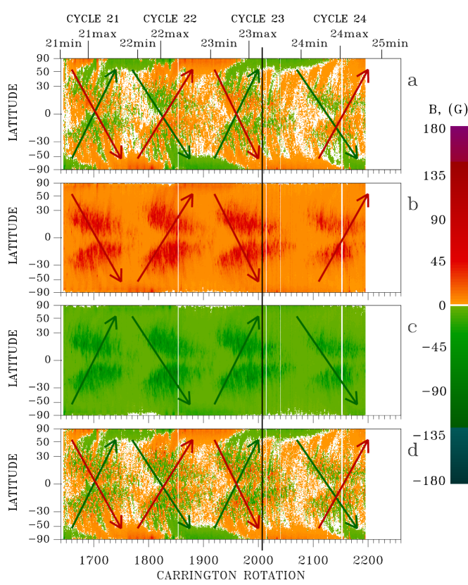
Figure 5.: Distributions of high-resolution photospheric magnetic fields from KPVT (CRs 1625 – 2007) and SOLIS (CRs 2008 – 2196) synoptic maps. (a) Butterfly diagram. Time-latitude distributions of longitude-averaged positive-polarity (b) and negative-polarity (c) magnetic fields. (d) Superposition of the distributions of positive- and negative-polarity magnetic fields shown in panels (b) and (c). Designations are the same as in Figure 1. Black vertical line marks the transition from KPVT to SOLIS in CR 2007.

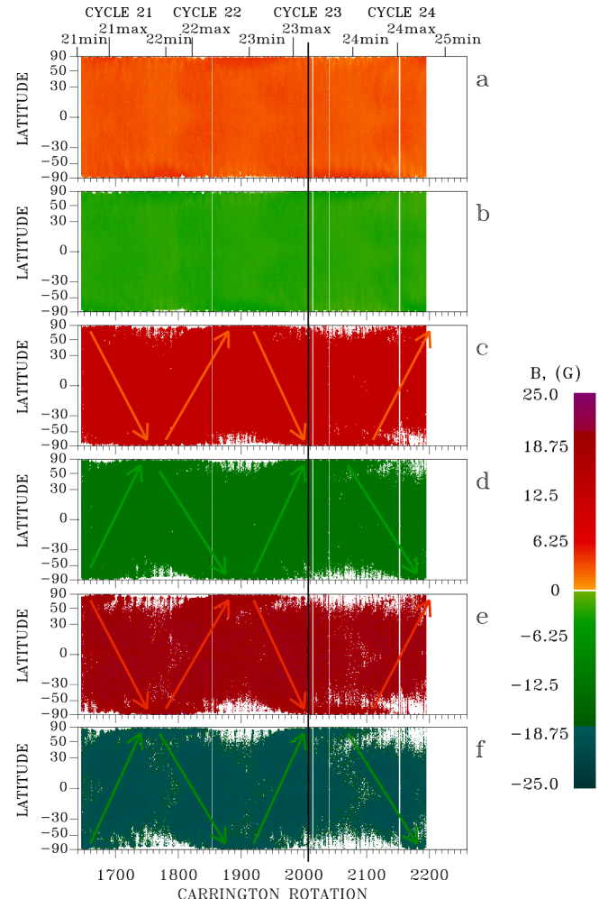
Figure 6.: Time-latitude distributions of high-resolution longitude-averaged low-strength and medium-strength positive- and negative-polarity photospheric magnetic fields in different ranges (KPVT, CRs 1625 – 2007 and SOLIS, CRs 2008 – 2196). (a) $0<B\leq 7$ G; (b) $-7\leq B<0$ G; (c) $10<B\leq 15$ G; (d) $-15\leq B<-10$ G; (e) $15<B\leq 25$ G; (f) $-25\leq B<-15$ G. Designations are the same as in Figure 5.

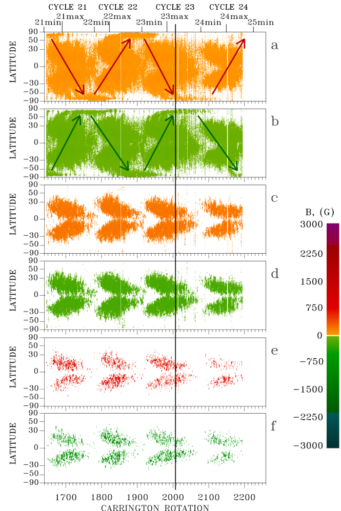
Figure 7.: Time-latitude distributions of high-resolution longitude-averaged high-strength positive- and negative-polarity photospheric magnetic fields in different ranges (KPVT, CRs 1625 – 2007 and SOLIS, CRs 2008 – 2196). (a) $25<B\leq 100$ G; (b) $-100\leq B<-25$ G; (c) $100<B\leq 500$ G; (d) $-500\leq B<-100$ G; (e) $B>500$ G; (f) $B<-500$ G. Designations are the same as in Figure 5.

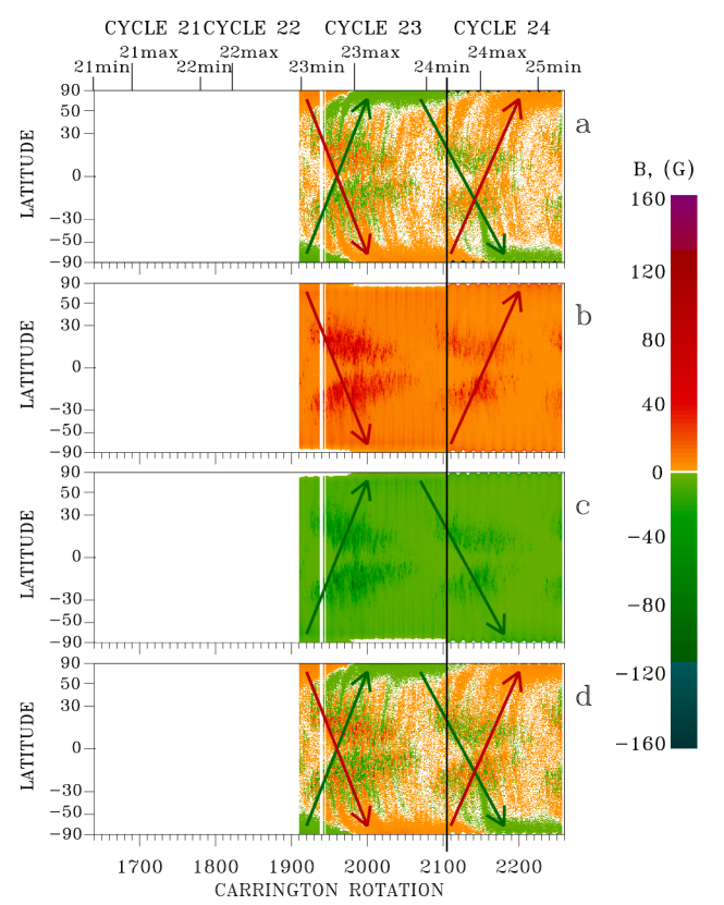
Figure 8.: Distributions of high-resolution photospheric magnetic fields from SOHO/MDI (CRs 1911 – 2104) and SDO/HMI (CRs 2105 – 2267) synoptic maps. (a) Butterfly diagram. Time-latitude distributions of longitude-averaged positive-polarity (b) and negative-polarity (c) magnetic fields. (d) Superposition of the distributions of positive- and negative-polarity magnetic fields shown in panels (b) and (c). Black vertical line marks the transition from SOHO/MDI to SDO/HMI in CR 2105. Designations are the same as in Figure 1.

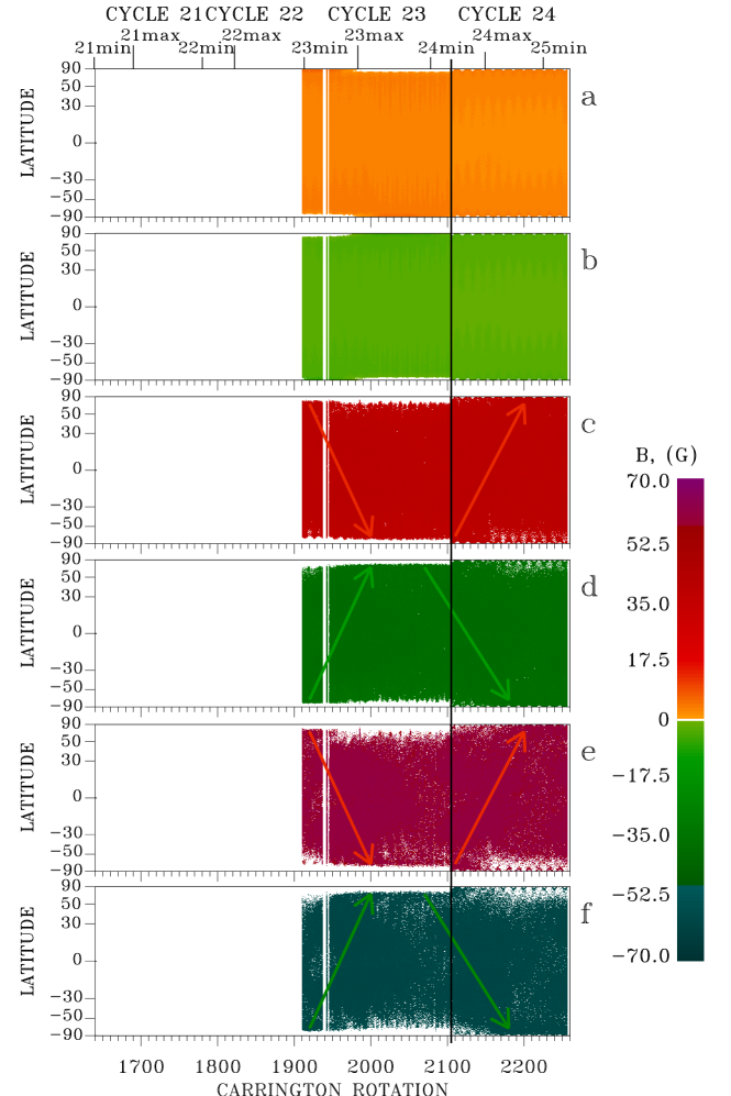
Figure 9.: Time-latitude distributions of high-resolution longitude-averaged low-strength and medium-strength positive- and negative-polarity photospheric magnetic fields (SOHO/MDI, CRs 1911 – 2104 and SDO/HMI, CRs 2105 – 2267). (a) $0<B\leq 7$ G; (b) $-7\leq B<0$ G; (c) $30<B\leq 50$ G; (d) $-50\leq B<-30$ G; (e) $50<B\leq 70$ G; (f) $-70\leq B<-50$ G. Designations are the same as in Figure 8.

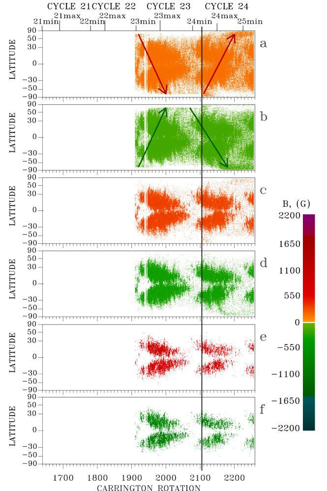
Figure 10.: Time-latitude distributions of high-resolution longitude-averaged high-strength positive- and negative-polarity photospheric magnetic fields in different ranges (SOHO/MDI, CRs 1911 – 2104 and SDO/HMI, CRs 2105 – 2267). (a) $100<B\leq 200$ G; (b) $-200\leq B<-100$ G; (c) $200<B\leq 500$ G; (d) $-500\leq B<-200$ G; (e) $B>500$ G; (f) $B<-500$ G. Designations are the same as in Figure 8.

The resolution of WSO magnetic fields is 3 arc-min. Therefore, WSO magnetic-field data show the dynamics of low-resolution large-scale magnetic fields. To investigate the distribution and meridional circulation of high-resolution magnetic fields, synoptic data from ground based KPVT and SOLIS and space SOHO/MDI and SDO/HMI observatories were used. Figure 5 shows the time-latitude distributions of longitude-averaged positive- and negative-polarity magnetic fields at high spatial resolution (KPVT, CRs 1625 – 2007 and SOLIS, CRs 2008 – 2196). Figure 6 shows that in the range of $0<\mid B\mid\leq 25$ G, and Figure 7 shows that for $\mid B\mid>25$ G. Figures 8 – 10 show similar time-latitude distributions constructed from the synoptic magnetic maps of SOHO/MDI (CRs 1911 – 2104) and SDO/HMI (CRs 2105 – 2267). HMI maps (3600$\times$1440 pixels) were recalculated to MDI scale (3600$\times$1080 pixels). To convert HMI magnetic field data to that of MDI, the conversion factor of 1.01 (Riley et al., 2014) was used.

Unlike WSO, the fine structure of the magnetic field distribution appears more clearly in the diagrams Figures 5 and 8. Comparison of Figures 1  –  10 shows that different data show a very similar distributions and meridional flows in similar magnetic field ranges, but the intensity of the magnetic fields greatly differs between the data sets. It should be noted that magnetic field distributions were analyzed on the basis of the synoptic maps of different independent observatories. Despite this, the results obtained using instruments with low and high spatial resolution are the same. Three types of magnetic field distributions and meridional circulations depending on the magnetic field strength were also identified. The first type are low-strength magnetic fields ($0<\mid B\mid\leq 7$ G, KPVT-SOLIS and MDI-HMI). They were almost cycle-independent and distributed evenly over the solar disk. The second type includes medium-strength magnetic fields ($10<\mid B\mid\leq 25$ G, KPVT-SOLIS and $30<\mid B\mid\leq 70$ G, MDI-HMI) High-resolution medium-strength magnetic fields also revealed wave-like, antiphase, pole-to-pole meridional circulation with a period of $\approx$22 years. They transport the new polarity magnetic field to the poles. The third type consists of strong magnetic fields ($\mid B\mid>100$ G, KPVT-SOLIS and $\mid B\mid>200$ G, MDI-HMI). High-strength magnetic fields show meridional circulation of active regions from high to low latitudes in the Northern and Southern hemispheres. Neither the leading nor the following polarity sunspot magnetic fields migrate to the poles in any of the magnetic field ranges.

From Figures 7(a and b) and  10(a and b) it follows that some high-latitude active region magnetic fields, whose polarity coincided with the polarity of the second type meridional circulation waves, i.e. medium-strength magnetic field flows, indicated by arrows in Figures 7(a and b) and 10(a and b), were picked up by the second type pole-to-pole meridional circulation waves and transported to the poles. Thus some active region magnetic fields participate in the solar pole field reversals, but they are not the main source of the new polarity magnetic fields at the solar poles.

5 Variations in the Magnetic Field Magnitudes of Different Type Meridional Circulations

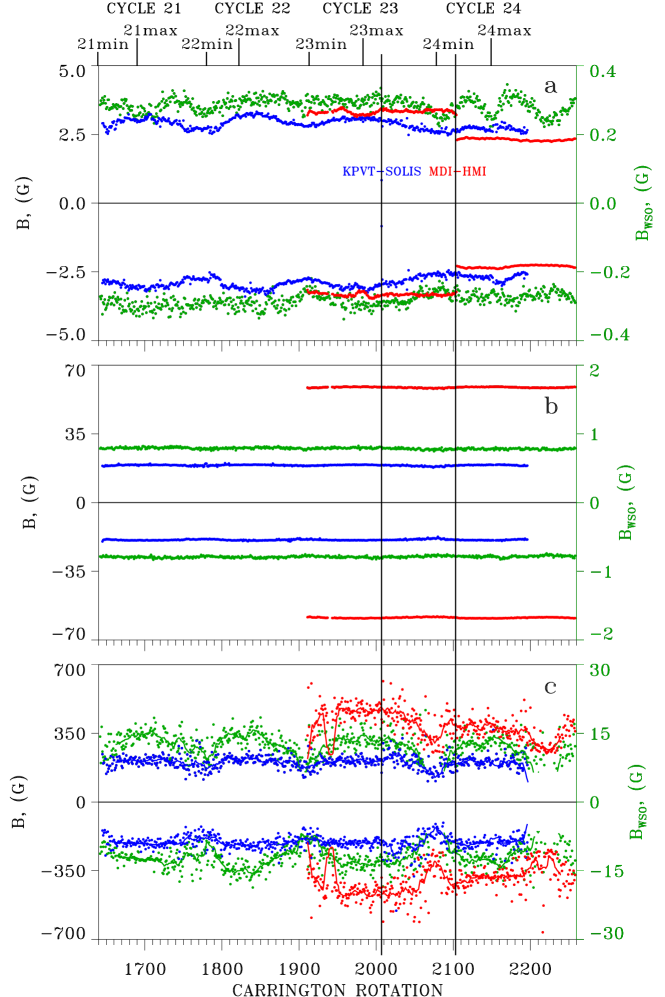
Figure 11.: Variations in the mean magnetic field strength. (a) $0<\mid B\mid\leq 0.6$ G (WSO); $0<\mid B\mid\leq 7$ G (KPVT-SOLIS and MDI-HMI); (b) $0.6<\mid B\mid\leq 1.0$ G (WSO); $10<\mid B\mid\leq 25$ G (KPVT-SOLIS); $30<\mid B\mid\leq 70$ G (MDI-HMI); (c) $\mid B\mid>7$ G (WSO); $\mid B\mid>100$ G (KPVT-SOLIS); $\mid B\mid>200$ G (MDI-HMI). Green denotes WSO data (right $y$ axes), blue denotes KPVT-SOLIS data, and red denotes MDI-HMI data. Dots represent CR-averaged data and thick lines represent seven-CR-averaged data. Solar cycles maxima and minima are marked at the top. The black vertical lines mark the transition from KPVT to SOLIS and from MDI to HMI.

Figure 11 shows the variations in the mean strength of magnetic fields in each CR for the selected magnetic-field ranges according to WSO (green), KPVT-SOLIS (blue), and MDI-HMI (red) data. Variations in the mean of low-strength magnetic fields (the first type) are shown in Figure 11(a) Variations in WSO ($0<\mid B\mid\leq 0.6$ G) data were insignificant in amplitude and did not coincide with the solar cycle variations of active region magnetic fields. They are minimal at cycles maxima. The mean magnetic field values of KPVT-SOLIS data ($0<\mid B\mid\leq 7$ G) increased slightly toward the maximum and decreased toward the minimum of each solar cycle. MDI-HMI low-strength magnetic fields did not reveal solar cycle variations at all.

The mean magnetic field values of the second type meridional circulation, i.e. the medium-strength wave-like, pole-to-pole positive- and negative-polarity magnetic field flows, are presented in Figure 11(b). The selected magnetic field ranges correspond to $0.6<\mid B\mid\leq 1.0$ G for WSO, $15<\mid B\mid\leq 25$ G for KPVT-SOLIS, and $50<\mid B\mid\leq 70$ G for MDI-HMI data. For the second type meridional circulation, the magnitudes of magnetic fields remained approximately at the same level at all solar cycle phases during Solar Cycles 21 – 24.

In Figure 11(c) the variations in the mean magnetic field of the third type meridional circulation (meridional flows of high-strength positive- and negative-polarity active region magnetic fields) are shown. The selected magnetic field ranges correspond to $\mid B\mid>7$ G for WSO, $\mid B\mid>100$ for KPVT-SOLIS, and $\mid B\mid>200$ G for and MDI-HMI. The solar cycle variations are clearly visible. The mean values of magnetic fields in these ranges increased to the maximum and decreased to the minimum of solar activity in each cycle.

The mean of magnetic fields calculated on the base of high-resolution synoptic maps, turn out to be low, since weak magnetic fields occupy larger areas in the synoptic maps and their contribution to the total magnetic field is higher. It should be noted that the MDI and HMI data in the range of $0<\mid B\mid\leq 7.0$ G did not agree well with each other despite the using of conversion coefficient. The values of magnetic fields according to the HMI data were much lower than those according to the MDI data. There is no such difference in other magnetic field ranges. This may indicate the nonlinearity of the relationship between the MDI and HMI magnetic field data.

6 Mean Latitudes and Velocities of Different Type Meridional Circulations

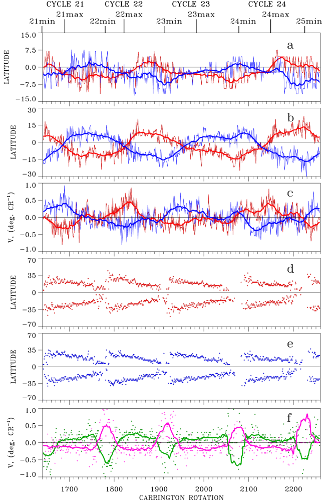
Figure 12.: Mean latitudes and velocities of different type meridional flows (WSO). Variations in the mean latitudes of low-strength positive- and negative-polarity magnetic fields in the range of $0<\mid B\mid\leq 0.6$ G (a). (b) Variations in the mean latitudes of medium-strength positive- and negative-polarity magnetic fields in the range of $0.8<\mid B\mid\leq 1.0$ G. (c) Velocities of medium-strength positive-polarity (red) and negative-polarity (blue) magnetic field flows. Variations in the mean latitudes of high-strength positive-polarity (d) and negative-polarity (e) magnetic fields in the range of $\mid B\mid>7$ G. (f) Velocities of the high-strength positive-polarity magnetic field flows in the North (green) and South (lilac) hemispheres. In (a) – (e) red indicates magnetic fields of positive polarity, and blue indicates that of negative polarity. Thin lines show the values averaged for each CR. Thick lines indicate the values averaged over 31 CRs.

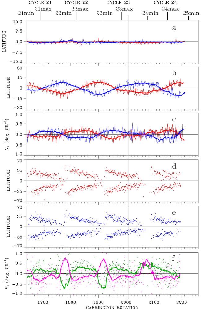
Figure 13.: Mean latitudes and velocities of different type meridional flows (KPVT-SOLIS). Variations in the mean latitudes of low-strength positive- and negative-polarity magnetic fields in the range of $0<\mid B\mid\leq 7$ G (a). (b) Variations in the mean latitudes of medium-strength positive- and negative-polarity magnetic fields in the range of $15<\mid B\mid\leq 25$ G. (c) Velocities of medium-strength positive-polarity (red) and negative-polarity (blue) magnetic field flows. Variations in the mean latitudes of high-strength positive-polarity (d) and negative-polarity (e) magnetic fields in the range of $\mid B\mid>500$ G. (f) Velocities of the high-strength positive-polarity magnetic field flows in the North (green) and South (lilac) hemispheres. Designations are the same as in Figure 12.

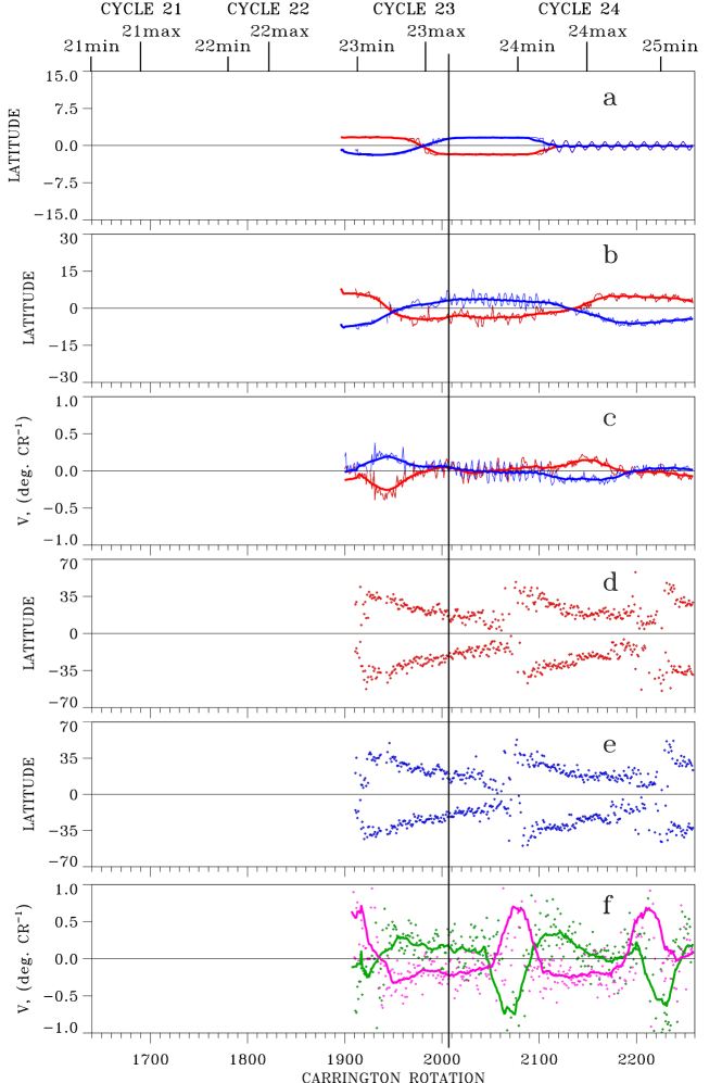
Figure 14.: Mean latitudes and velocities of different type meridional flows (MDI-HMI). Variations in the mean latitudes of low-strength positive- and negative-polarity magnetic fields in the range of $0<\mid B\mid\leq 7$ G (a). (b) Variations in the mean latitudes of medium-strength positive- and negative-polarity magnetic fields in the range of $30<\mid B\mid\leq 50$ G. (c) Velocities of medium-strength positive-polarity (red) and negative-polarity (blue) magnetic field flows. Variations in the mean latitudes of high-strength positive-polarity (d) and negative-polarity (e) magnetic fields in the range of $\mid B\mid>500$ G. (f) Velocities of the high-strength positive-polarity magnetic field flows in the North (green) and South (lilac) hemispheres. Designations are the same as in Figure 12.

Figures 12 – 14 show the variations in the mean latitudes and velocities of different type meridional circulations in Solar Cycles 21 – 24. The mean latitudes were calculated for each CR from the corresponding time-latitude distributions of magnetic fields. Variations in the mean latitudes of low-strength positive- and negative-polarity magnetic fields are shown in Figures 12(a), 13(a), and 14(a). Their mean latitudes were near the equator. Positive- and negative-polarity magnetic fields varied in anti phase, but their variations had no any cycle dependence.

Variations in the mean latitudes of the second type meridional circulation flows are shown in Figures 12(b), 13(b), and 14(b). Wave-like flows were located at low latitudes during solar activity maxima. The average latitude of the meridional magnetic flows of both polarities increased with a decrease in solar activity to the minimum of each cycle in the northern and southern hemispheres. Waves of positive and negative polarity remained at high latitudes in each hemisphere until the rising phase of the next cycle. It should be noted, that waves of the second type meridional flows occupied a wide range of latitudes in each CR. Therefore, variations in their mean latitudes indicate the general direction of the wave migration.

In Figures 12(c), 13(c), and 14(c) the velocity of the second type meridional flows in degrees per CR are shown. Velocities were higher when meridional the flows were at low latitudes and they crossed the equator migrating from the North (South) to the South (North) hemisphere during solar activity maximum. Velocities decreased to minimal values during the periods when the flows were at high latitudes during solar activity minimum. In the polar regions, the meridional flows seem to turn around and their velocity decreases to zero.

Figures 12(d, e), 13(d, e), and 14(d, e) show variations in the mean latitudes of the third type meridional circulation, i.e. the meridional circulation of high-strength positive- and negative-polarity magnetic fields. Their meridional flows reflect the well known solar cycle dynamics of active regions. They appeared at high latitudes during the rising phases of solar activity and drifted towards low latitudes. In Figures 12(f), 13(f), and 14(f) the velocities (degree per CR) of the third type meridional circulation flows are presented. The latitudes of meridional flows of high-strength positive- and negative-polarity magnetic fields are almost identical. When their latitudinal distributions are superimposed, they coincide with each other with great accuracy. Therefore the velocities of positive-polarity magnetic fields in the North and South hemispheres are presented. The maximal velocities were at the rising solar cycle phases in all cycles. With cycle activity the velocities decreased. Comparison of meridional circulation of medium-strength magnetic fields with that of high-strength shows that active regions did not form when the second type meridional flows were at the highest latitudes in each cycle. Active regions began to form when the latitudes of antiphase meridional flow waves of medium-strength magnetic fields shifted to lower latitudes as they drifted to the opposite hemispheres. The formation of active regions stopped when the wave meridional flows of medium-strength positive- and negative-polarity magnetic fields migrated away from the equator and approached the opposite poles.

The results indicate that both low-resolution large-scale (WSO) and high-resolution (KPVT-SOLIS and MDI-HMI) magnetic field data show similar solar cycle changes in the mean latitude variations of different strength magnetic fields and the velocities of their meridional circulations.

It should be noted, that the WSO mean latitudes were shifted to the South hemisphere in all ranges. It seems to be the instrumental effect. There were no such shift neither in KPVT-SOLIS nor in MDI-HMI data.

7 Discussion

Three different types of time-latitude distributions and meridional circulations of solar magnetic fields were revealed. They depend on the strength of the photospheric magnetic fields. Both low-resolution large-scale magnetic field data (WSO) and high-resolution data (KPVT-SOLIS and MDI-HMI) show the same three types of photospheric magnetic field dynamics, but the magnetic field strength values are different due to different instruments. The first type includes low-strength magnetic fields. Low-strength magnetic fields are distributed throughout the solar surface, but their properties and spatial-temporal variations are not yet well known. Currently, it is unclear what mechanism underlies the origin and dynamics of weak magnetic fields. It is unclear whether they are the remnants of the active region magnetic fields or the result of a turbulent small-scale dynamo. In the latter case, their distribution and variations in the strength of their magnetic field should not coincide with that in the magnetic fields of active regions. The small-scale dynamo does not depend on the large-scale dynamo. The results show that they were distributed evenly across the solar disk, their time-latitude distribution and the mean value of their magnetic field strength did not change during solar cycles from the minimum to maximum of solar activity. Their behavior is almost cycle-independent. This is consistent with the results obtained from daily magnetograms by (Kleint et al., 2010; Buehler, Lagg, and Solanki, 2013; Lites, Centeno, and McIntosh, 2014; Jin and Wang, 2015a, b). Thus, low-strength magnetic fields show little variation over space and time that was not coincide with that of active regions, indicating that they are predominantly governed by a process that is independent of the active region solar cycle. The results indicate that low-strength magnetic fields are not a product of the decay of active region magnetic fields. This supports the notion that low-strength magnetic fields caused by a turbulent small-scale dynamo.

The second type meridional circulation is demonstrated by medium-strength magnetic fields. Positive- and negative-polarity magnetic fields reveal wavy antiphase meridional flows from pole to pole with a period of approximately 22 years. They cross the equator during the maximum of solar activity. Cycle evolution of coronal holes (CHs) revealed some temporal and spatial regularities (Bilenko, 2002; Bilenko and Tavastsherna, 2016) that match well the wave-like pole-to-pole meridional circulation of medium-strength magnetic fields. In Bilenko (2002) the pole-to-pole antiphase meridional drift was revealed for CHs associated with positive- and negative-polarity photospheric magnetic fields. In Bilenko and Tavastsherna (2016) we found two different type waves of non-polar CHs. The first are short waves that trace the poleward movement of unipolar magnetic fields from approximately $35^{\circ}$ latitude to the corresponding pole in each hemisphere. The second type of non-polar CH waves forms two antiphase sinusoidal branches associated with the positive- and negative-polarity photospheric magnetic fields with a period of $\approx$268 CRs (22 years). These CH waves completely coincide with the meridional flows of the medium-strength positive- and negative-polarity photospheric magnetic fields revealed in Sections 3 and 4. The study of CHs by other authors confirmed our results. Pevtsov and Abramenko (2010) described the observational evidence of a transport of one CH across the equator from one solar polar region to the other. Huang, Lin, and Lee (2017) found that during the rising phase, the opposite directed open magnetic fluxes (CH regions), showed pole-to-pole trans-equatorial migrations in opposite directions. Maghradze et al. (2022) also found sinusoidal cyclic migration of the centers of CH activity with opposite directed magnetic fluxes from pole to pole across the solar equator.

CHs are considered to be good traces of the solar large-scale, global magnetic field cycle evolution (Stix, 1977; Bagashvili et al., 2017; Bilenko and Tavastsherna, 2017, 2020). Thus, medium-strength magnetic fields reflect the solar global magnetic field cycle evolution. Cycle changes in the latitude location of the CH waves coincide with that of the axisymmetric component of the solar dipole ($g_{1}^{0}$) (Bilenko and Tavastsherna, 2016). When both CH branches were above $\approx\pm 35^{\circ}$ latitude, the zonal structure was observed. When two branches of positive- and negative-polarity magnetic fields and CHs move below $\approx\pm 35^{\circ}$ latitude, the zonal structure of the GMF changes to sectorial one (Bilenko and Tavastsherna, 2016). This moment coincides with the beginning of the formation of high-strength active region magnetic fields. Apparently, the formation of high-strength magnetic fields is somehow associated with the second type wave-like meridional circulation, i.e. medium-strength magnetic field dynamics.

It is important to note, that Komm (2022) determined the direction and amplitude of cross-equatorial flows below the solar surface. They found that the cross-equatorial flow was mainly southward during Solar Cycle 23 and mainly northward during Solar Cycle 24. At depths less than 7 Mm, the average velocity was -1.1 $\pm$ 0.2 m s^-1 in Solar Cycle 23 and +1.3$\pm$0.1 m s^-1 in Solar Cycle 24. At the beginning of Solar Cycle 25, the cross-equatorial flow changed sign again. They concluded, that the subsurface cross-equatorial flow was nonzero and caused by the inflows associated with active regions located close to the equator and it was directed to the hemisphere with the greater amount of flux. But, apparently, these subsurface meridional flows were associated with the second type meridional circulation of medium-strength magnetic fields. The second type meridional circulation can be associated with processes occurring at the base of the convective zone. Jones (2005), for example, noted that CHs may be rooted as deep as the base of the convection zone.

The third type is the meridional circulation of high-strength magnetic fields, i.e. fields of active regions. Both positive- and negative-polarity high-strength magnetic fields migrate from high latitudes towards the equator in each cycle. Neither the magnetic fields of the leading sunspot polarity nor the following ones migrate to the poles. It is interesting to note that using the Kodaikanal Observatory archives for 1906 – 1987 and the Mt. Wilson Observatory archives for 1917 – 1985, Sivaraman et al. (2010) found that the latitudinal drifts (or the meridional flows) of spot groups classified into three categories of area: 0 – 5, 5 – 10, and $>$10 millionths of the solar hemisphere were directed equator ward in both the North and South hemispheres. The equator ward drift velocity increases from almost zero at $35^{\circ}$ latitude in both hemispheres reaches maximum around $20^{\circ}$ latitude and slows down towards zero near the equator Sivaraman et al. (2010). Consequently, both the active regions themselves and their magnetic fields migrate from latitudes of $35^{\circ}$ to the equator, and not to the poles. Some of the high-latitude active region magnetic fields were captured by the second type wave-like flows in their drift to the appropriate pole and transported to the poles. However, the magnetic fields of active regions are not the main ones in the process of the solar polar field reversal.

So, the observed magnetic-field cycle dynamics is a superposition of tree different type time-latitude distributions and meridional circulations. Therefore, the solar cycle is governed by different types of dynamo. Benevolenskaya (1998) proposed a new dynamo model to explain the solar magnetic cycle that consists of two main periodic components: a low-frequency component (Hale’s 22 yr cycle) and a high-frequency component (quasi-biennial cycle). The essence of the model is that two dynamo sources are at different levels. The first is located near the bottom of the convection zone, and the other is near the top. It is possible that the assumption of the joint operation of different types of dynamos at different levels in the convective zone and near the surface will make it possible to better explain the observed distributions of magnetic fields of different strengths and their solar cycle dynamics.

8 Conclusions

Meridional circulation of the solar magnetic fields were analyzed using synoptic magnetic field data from ground based WSO, NSO KPVT, and SOLIS/VSM and space based SOHO/MDI and SDO/HMI observatories for Solar Cycles 21 – 24. It have been found that cycle variations of low-, middle-, and hight-strength magnetic fields significantly different. Depending on the intensity of the photospheric magnetic fields, three types of time-latitude distributions and meridional circulations were identified for both low and high spatial resolution data.

The first type includes low-strength magnetic fields ($0<\mid B\mid\leq 0.6$ G for WSO and $0<\mid B\mid\leq 7$ G for KPVT-SOLIS and MDI-HMI). They were distributed evenly across latitude and their average strength weakly depended on cycle variations of the active region magnetic fields. These fields are believed to be determined by a small-scale dynamo.

The second is medium-strength magnetic field meridional circulation ($0.6<\mid B\mid\leq 1$ G for WSO, $10<\mid B\mid\leq 25$ G for KPVT-SOLIS, and $30<\mid B\mid\leq 70$ G for MDI-HMI). Fields of positive and negative polarity revealed a wave-like antiphase meridional circulation from pole to pole with a period of approximately 22 years. The velocity of meridional flows were slower at the minima of solar activity, when they were at high latitudes in the opposite hemispheres, and maximal at the solar cycle maxima, when the positive- and negative-polarity waves crossed the equator. The flows were more pronounced in large-scale magnetic field data and in magnetic fields calculated at the source surface. The meridional circulation of these fields reflects the solar global magnetic field dynamics and determines the solar polar field reversal.

The third type meridional circulation includes high-strength magnetic fields, the fields of active regions ($\mid B\mid>7$ G for WSO, $\mid B\mid>100$ G for KPVT-SOLIS, and $\mid B\mid>200$ G for MDI-HMI). Magnetic fields of positive and negative polarity were distributed symmetrically in both hemispheres with respect to the equator. Active region magnetic fields of both leading and following sunspot polarity migrate from high to low latitudes in all magnetic field ranges. The velocities of these meridional flows were higher at the rising and maxima phases than at the minima.

The magnetic fields of active regions are not the main source of magnetic fields that determine the solar polar field reversal. The magnetic fields of some high-latitude active regions picked up by the meridional wave-like flows (meridional circulation of the second type) of the corresponding polarity during the rising solar cycle phases and transported along with the flows to the poles.

The butterfly diagram is just the result of a superposition of cyclically changing meridional flows of different strength positive- and negative-polarity magnetic fields. The various details and structures in the butterfly diagram, for example poleward surges, are the result of the domination of one of the polarities.

Acknowledgements

Wilcox Solar Observatory data used in this study was obtained via the web site http://wso.stanford.edu at 2023:04:28_12:04:38 PDT courtesy of J.T. Hoeksema. The Wilcox Solar Observatory is currently supported by NASA.

NSO/Kitt Peak magnetic data used here are produced cooperatively by NSF/NOAO, NASA/GSFC, and NOAA/SEL.

This work utilizes SOLIS data obtained by the NSO Integrated Synoptic Program (NISP), managed by the National Solar Observatory, which is operated by the Association of Universities for Research in Astronomy (AURA), Inc. under a cooperative agreement with the National Science Foundation.

SOHO/MDI data were also used. SOHO is a project of international cooperation between ESA and NASA.

HMI data are courtesy of the Joint Science Operations Center (JSOC) Science Data Processing team at Stanford University.

References

- Altschuler and Newkirk (1969) Altschuler, M.D., Newkirk, J. G.: 1969, Magnetic Fields and the Structure of the Solar Corona. I: Methods of Calculating Coronal Fields. Sol. Phys. 9, 131. DOI.
- Bagashvili et al. (2017) Bagashvili, S.R., Shergelashvili, B.M., Japaridze, D.R., Chargeishvili, B.B., Kosovichev, A.G., Kukhianidze, V., Ramishvili, G., Zaqarashvili, T.V., Poedts, S., Khodachenko, M.L., De Causmaecker, P.: 2017, Statistical Properties of Coronal Hole Rotation Rates: Are they Linked to the Solar Interior? A&A 603, id. A134, 8 pp. DOI.
- Basu and Antia (2003) Basu, S., Antia, H.M.: 2003, Changes in Solar Dynamics from 1995 to 2002. ApJ 585, 553. DOI.
- Basu and Antia (2010) Basu, S., Antia, H.M.: 2010, Characteristics of Solar Meridional Flows During Solar Cycle 23. ApJ 717, 488. DOI.
- Benevolenskaya (1998) Benevolenskaya, E.E.: 1998, A model of the Double Magnetic Cycle of the Sun. ApJ 509, L49. DOI.
- Bilenko (2002) Bilenko, I.A.: 2002, Coronal Holes and the Solar Polar Field Reversal. A&A 396, 657. DOI.
- Bilenko and Tavastsherna (2016) Bilenko, I.A., Tavastsherna, K.S.: 2016, Coronal Hole and Solar Global Magnetic Field Evolution in 1976-2012. Sol. Phys. 291, 2329. DOI.
- Bilenko and Tavastsherna (2017) Bilenko, I.A., Tavastsherna, K.S.: 2017, Coronal Holes as Tracers of the Sun’s Global Magnetic Field in Cycles 21-23 of Solar Activity. Geomagnetism and Aeronomy 57, 803. DOI.
- Bilenko and Tavastsherna (2020) Bilenko, I.A., Tavastsherna, K.S.: 2020, Formation and Evolutionary Changes of Coronal Holes in the Growth Phase of Cycle 23. Geomagnetism and Aeronomy 60, 421. DOI.
- Buehler, Lagg, and Solanki (2013) Buehler, D., Lagg, A., Solanki, S.K.: 2013, Quiet Sun Magnetic Field Observed by Hinode: Support for a Local Dynamo. A&A 555, id. A33, 10 pp. DOI.
- Charbonneau (2020) Charbonneau, P.: 2020, Dynamo Models of the Solar Cycle. Living Reviews in Solar Physics 17, 4. DOI.
- Chou and Dai (2001) Chou, D.-Y., Dai, D.-C.: 2001, Solar Cycle Variations of Subsurface Meridional Flow in the Sun. ApJ 559, L175. DOI.
- Duvall and Jr. (1979) Duvall, T.L., Jr.: 1979, Large-Scale Solar Velocity Fields. Sol. Phys. 63, 3. DOI.
- Duvall et al. (1977) Duvall, T.L., Jr., Wilcox, J.M., Svalgaard, L., Scherrer, P.H., McIntosh, P.S.: 1977, Comparison of Ha Synoptic Charts with the Large-scale Solar Magnetic Field as Observed at Stanford. Sol. Phys. 55, 63. DOI.
- Gizon (2004) Gizon, L.: 2004, Helioseismology of Time-Varying Flows Through The Solar Cycle. Sol. Phys. 224, 217. DOI.
- Hanasoge (2022) Hanasoge, S.M.: 2022, Surface and Interior Meridional Circulation in the Sun. Living Reviews in Solar Physics 19, 1. DOI.
- Hathaway (1996) Hathaway, D.H.: 1996, Doppler Measurements of the Sun’s Meridional Flow. ApJ 460, 1027. DOI.
- Hathaway and Rightmire (2010) Hathaway, D.H., Rightmire, L.: 2010, Variations in the Sun’s Meridional Flow over a Solar Cycle. Science 327, 1350. DOI.
- Hathaway and Upton (2014) Hathaway, D.H., Upton, L.: 2014, The Solar Meridional Circulation and Sunspot Cycle Variability. J. Geophys. Res. 119, 3316. DOI.
- Hoeksema and Scherrer (1988) Hoeksema, J.T., Scherrer, P.H.: 1988, An Atlas of Photospheric Magnetic Field Observations and Computed Coronal Magnetic Fields: 1976-1985. Solar - Geophysical Date (SGD) 105, no. 383.
- Hoeksema, Wilcox, and Scherrer (1983) Hoeksema, J.T., Wilcox, J.M., Scherrer, P.H.: 1983, The Structure of the Heliospheric Current Sheet: 1978-1982. J. Geophys. Res. 88, 9910. DOI.
- Howard (1979) Howard, R.: 1979, Evidence for Large-scale Velocity Features on the Sun. ApJ 228, L45. DOI.
- Howard and Gilman (1986) Howard, R., Gilman, P.A.: 1986, Meridional Motions of Sunspots and Sunspot Groups. ApJ 307, 389. DOI.
- Huang, Lin, and Lee (2017) Huang, G.-H., Lin, C.-H., Lee, L.C.: 2017, Solar Open Flux Migration from Pole to Pole: Magnetic Field Reversal. Scientific Reports 7, id. 9488. DOI.
- Imada et al. (2020) Imada, S., Matoba, K., Fujiyama, M., Iijima, H.: 2020, Solar Cycle-related Variation in Solar Differential Rotation and Meridional Flow in Solar Cycle 24. Earth, Planets and Space 72, article id.182. DOI.
- Jiang et al. (2014) Jiang, J., Hathaway, D.H., Cameron, R.H., Solanki, S.K., Gizon, L., Upton, L.: 2014, Magnetic Flux Transport at the Solar Surface. Space Sci. Rev. 186, 491. DOI.
- Jin and Wang (2015a) Jin, C.L., Wang, J.X.: 2015a, Does the Variation of Solar Intra-network Horizontal Field Follow Sunspot Cycle? ApJ 807, article id. 70, 6 pp. DOI.
- Jin and Wang (2015b) Jin, C.L., Wang, J.X.: 2015b, Solar Cycle Variation of the Inter-network Magnetic Field. ApJ 806, article id. 174, 6 pp. DOI.
- Jones (2005) Jones, H.P.: 2005, Magnetic Fields and Flows in Open Magnetic Structures. In: Sankarasubramanian, K., Penn, M., Pevtsov, A. (eds.) Large-scale Structures and their Role in Solar Activity, Astron. Soc. Pac. CS-346, 229, 229.
- Jones et al. (1992) Jones, H.P., Duvall, T.L., Jr., Harvey, J.W., Mahaffey, C.T., Schwitters, J.D., Simmons, J.E.: 1992, The NASA/NSO Spectromagnetograph. Sol. Phys. 139, 211. DOI.
- Karak (2023) Karak, B.B.: 2023, Models for the Long-term Variations of Solar Activity. Living Reviews in Solar Physics 20, 3. DOI.
- Keller, Harvey, and Giampapa (2003) Keller, C.U., Harvey, J.W., Giampapa, M.S.: 2003, SOLIS: An Innovative Suite of Synoptic Instruments. In: Keil, S.L., Avakyan, S.V. (eds.) Innovative Telescopes and Instrumentation for Solar Astrophysics, SPIE 4853, 194. DOI.
- Kleint et al. (2010) Kleint, L., Berdyugina, S.V., Shapiro, A.I., Bianda, M.: 2010, Solar Turbulent Magnetic Fields: Surprisingly Homogeneous Distribution During the Solar Minimum. A&A 524, A37. DOI.
- Komm (2022) Komm, R.: 2022, Is the Subsurface Meridional Flow Zero at the Equator? Sol. Phys. 297, article id.99. DOI.
- Komm, Howard, and Harvey (1993) Komm, R.W., Howard, R.F., Harvey, J.W.: 1993, Meridional Flow of Small Photospheric Magnetic Features. Sol. Phys. 147, 207. DOI.
- Lites, Centeno, and McIntosh (2014) Lites, B.W., Centeno, R., McIntosh, S.W.: 2014, The Solar Cycle Dependence of the Weak Internetwork Flux. Publ. Astron. Soc. Jpn. 66, id.S4 14 pp. DOI.
- Livingston et al. (1976a) Livingston, W.C., Harvey, J., Pierce, A.K., Schrage, D., Gillespie, B., Simmons, J., Slaughter, C.: 1976a, Kitt Peak 60-cm Vacuum Telescope. Appl. Opt. 15, 33. DOI.
- Livingston et al. (1976b) Livingston, W.C., Harvey, J., Slaughter, C., Trumbo, D.: 1976b, Solar Magnetograph Employing Integrated Diode Arrays. Appl. Opt. 15, 40. DOI.
- Maghradze et al. (2022) Maghradze, D.A., Chargeishvili, B.B., Japaridze, D.R., Oghrapishvili, N.B., Chargeishvili, K.B.: 2022, Long-Term Variation of Coronal Holes Latitudinal Distribution. MNRAS 511, 5217. DOI.
- Petrovay (2020) Petrovay, K.: 2020, Solar Cycle Prediction. Living Reviews in Solar Physics 17, 2. DOI.
- Pevtsov and Abramenko (2010) Pevtsov, A.A., Abramenko, V.I.: 2010, Transport of Open Magnetic Flux Between Solar Polar Regions. In: Kosovichev, A.G., Andrei, A.H., Rozelot, J.-P. (eds.) Solar and Stellar Variability: Impact on Earth and Planets, Proceedings of the International Astronomical Union, IAU Symposium, Volume 264, 210. DOI.
- Pietarila et al. (2013) Pietarila, A., Bertello, L., Harvey, J.W., Pevtsov, A.A.: 2013, Comparison of Ground-Based and Space-Based Longitudinal Magnetograms. Sol. Phys. 282, 91. DOI.
- Rightmire-Upton, Hathaway, and Kosak (2012) Rightmire-Upton, L., Hathaway, D.H., Kosak, K.: 2012, Measurements of the Sun’s High-latitude Meridional Circulation. ApJ 761, article id. L14, 4 pp. DOI.
- Riley et al. (2014) Riley, P., Ben-Nun, M., Linker, J.A., Mikic, Z., Svalgaard, L., Harvey, J., Bertello, L., Hoeksema, T., Liu, Y., Ulrich, R.: 2014, A Multi-Observatory Inter-Comparison of Line-of-Sight Synoptic Solar Magnetograms. Sol. Phys. 289, 769. DOI.
- Schatten, Wilcox, and Ness (1969) Schatten, K.H., Wilcox, J.M., Ness, N.F.: 1969, A Model of Interplanetary and Coronal Magnetic Fields. Sol. Phys. 6, 442. DOI.
- Scherrer et al. (1977) Scherrer, P.H., Wilcox, J.M., Svalgaard, L., Duvall, T.L., Jr., Dittmer, P.H., Gustafson, E.: 1977, The Mean Magnetic Field of the Sun: Observations at Stanford. Sol. Phys. 54, 353. DOI.
- Scherrer et al. (1995) Scherrer, P.H., Bogart, R.S., Bush, R.I., Hoeksema, J.T., Kosovichev, A.G., Schou, J., Rosenberg, W., Springer, L., Tarbell, T.D., Title, A., Wolfson, C.J., Zayer, I., MDI Engineering Team: 1995, The Solar Oscillation Investigation - Michelson Doppler Imager. Sol. Phys. 162, 129. DOI.
- Scherrer et al. (2012) Scherrer, P.H., Schou, J., Bush, R.I., Kosovichev, A.G., Bogart, R.S., Hoeksema, J.T., Liu, Y., Duvall, T.L., Jr., Zhao, J., Title, A.M., Schrijver, C.J., Tarbell, T.D., Tomczyk, S.: 2012, The Helioseismic and Magnetic Imager (HMI) Investigation for the Solar Dynamics Observatory (SDO). Sol. Phys. 275, 207. DOI.
- Schou et al. (2012) Schou, J., Scherrer, P.H., Bush, R.I., et al.: 2012, Design and Ground Calibration of the Helioseismic and Magnetic Imager (HMI) Instrument on the Solar Dynamics Observatory (SDO). Sol. Phys. 275, 229. DOI.
- Schroeter and Woehl (1975) Schroeter, E.H., Woehl, H.: 1975, Differential Rotation, Meridional and Random Motions of the Solar Ca+ network. Sol. Phys. 42, 3. DOI.
- Sheeley (2005) Sheeley, N.R.J.: 2005, Surface Evolution of the Sun’s Magnetic Field: A Historical Review of the Flux-Transport Mechanism. Living Reviews in Solar Physics 2, 5. DOI.
- Sivaraman et al. (2010) Sivaraman, K.R., Sivaraman, H., Gupta, S.S., Howard, R.F.: 2010, Return Meridional Flow in the Convection Zone from Latitudinal Motions of Umbrae of Sunspot Groups. Sol. Phys. 266, 247. DOI.
- Snodgrass and Dailey (1996) Snodgrass, H.B., Dailey, S.B.: 1996, Meridional Motions of Magnetic Features in the Solar Photosphere. Sol. Phys. 163, 21. DOI.
- Stix (1977) Stix, M.: 1977, Coronal Holes and the Large-scale Solar Magnetic Field. A&A 59, 73.
- Sudar et al. (2014) Sudar, D., Skokić, I., Ruždjak, D., Brajša, R., Wöhl, H.: 2014, Tracing Sunspot Groups to Determine Angular Momentum Transfer on the Sun. MNRAS 439, 2377. DOI.
- Sudar et al. (2016) Sudar, D., Saar, S.H., Skokić, I., Poljančić Beljan, I., Brajša, R.: 2016, Meridional Motions and Reynolds Stress from SDO/AIA Coronal Bright Points Data. A&A 587, id A29 6 pp. DOI.
- Topka et al. (1982) Topka, K., Moore, R., Labonte, B.J., Howard, R.: 1982, Evidence for a Poleward Meridional Flow on the Sun. Sol. Phys. 79, 231. DOI.
- Virtanen and Mursula (2016) Virtanen, I., Mursula, K.: 2016, Photospheric and Coronal Magnetic Fields in Six Magnetographs I. Consistent Evolution of the Bashful Ballerina. A&A 591, A78. DOI.
- Virtanen and Mursula (2017) Virtanen, I., Mursula, K.: 2017, Photospheric and Coronal Magnetic Fields in Six Magnetographs II. Harmonic Scaling of Field Intensities. A&A 604, A7. DOI.
- Virtanen and Mursula (2019) Virtanen, I., Mursula, K.: 2019, Photospheric and Coronal Magnetic Fields in Six Magnetographs III. Photospheric and Coronal Magnetic Fields in 1974-2017. A&A 626, A67. DOI.
- Vršnak et al. (2003) Vršnak, B., Brajša, R., Wöhl, H., Ruždjak, V., Clette, F., Hochedez, J.-F.: 2003, Properties of the Solar Velocity Field Indicated by Motions of Coronal Bright Points. A&A 404, 1117. DOI.
- Zhao et al. (2013) Zhao, J., Bogart, R.S., Kosovichev, A.G., Duvall, T.L., Jr., Hartlep, T.: 2013, Detection of Equatorward Meridional Flow and Evidence of Double-cell Meridional Circulation inside the Sun. ApJ 774, article id. L29, 6 pp. DOI.