Thermalization rate of polaritons in strongly-coupled molecular systems

Abstract

Polariton thermalization is a key process in achieving light-matter Bose–Einstein condensation, spanning from solid-state semiconductor microcavities at cryogenic temperatures to surface plasmon nanocavities with molecules at room temperature. Originated from the matter component of polariton states, the microscopic mechanisms of thermalization are closely tied to specific material properties. In this work, we investigate polariton thermalization in strongly-coupled molecular systems. We developed a microscopic theory addressing polariton thermalization through electron-phonon interactions (known as vibronic coupling) with low-energy molecular vibrations. This theory presents a simple analytical method to calculate the temperature-dependent polariton thermalization rate, utilizing experimentally accessible spectral properties of bare molecules, such as the Stokes shift and temperature-dependent linewidth of photoluminescence, in conjunction with well-known parameters of optical cavities. Our findings demonstrate remarkable agreement with recent experimental reports of nonequilibrium polariton condensation in both ground and excited states, and explain the thermalization bottleneck effect observed at low temperatures. This study showcases the significance of vibrational degrees of freedom in polariton condensation and offers practical guidance for future experiments, including the selection of suitable material systems and cavity designs.

I Introduction

Electronic and vibrational states hold a central place in the molecular systems that drive photo-induced processes in nature [1] and underlie many of the technologies we interact with on a daily basis [2]. Despite the large energetic disparity between electronic and vibrational states, they can undergo substantial electron-phonon interactions, known as vibronic coupling [3, 4]. This coupling defines absorption and emission spectra of molecular systems [5, 6, 7] and shapes the relaxation dynamics at the microscopic level [8, 9, 10]. When placed inside optical cavities, molecules can engage in strong light-matter interactions, leading to an effective tripartite interaction [11, 12, 13]. This results in the formation of new eigenstates, known as vibronic-type exciton-polaritons [14, 13], also referred as polaron polaritons in molecular exciton-plasmon systems [15, 16]. Due to the typically strong vibronic coupling, these polariton states are prevalent in molecular systems. As hybrid light-matter states, polaritons inherit properties from both molecules and the cavity electromagnetic field. From the latter, they acquire a small effective mass and a typically short lifetime $\sim 100$ fs.

As bosons, polaritons can form Bose–Einstein condensate (BEC), where their small effective mass and low density of states favor condensation at elevated temperatures [17]. However, their short lifetime means that polariton BEC in molecular systems is significantly out of thermal equilibrium, requiring constant re-population of the reservoir to compensate for polariton losses [18]. Despite the intrinsic nonequilibrium nature of polariton condensates, they can still achieve some form of effective local equilibrium with the environment. This equilibrium is defined by the complex interplay of gain, loss, and thermalization within the polariton system. Recent theoretical reports have rigorously demonstrated this regime through an exact solution for the density matrix in the fast thermalization limit [19, 20]. While fast thermalization is a reasonable approximation above the condensation threshold, it is not sufficiently accurate at the onset of polariton BEC. Therefore, understanding polariton thermalization is pivotal for the physics of light-matter condensates in molecular systems. The actual microscopic mechanisms behind polariton thermalization remain an open question in the field. Recently, Satapathy et al. have shed light on the nature of thermalization in organic microcavities, experimentally demonstrating the central role of the emission Stokes shift of molecules in polariton thermalization towards the BEC [21].

The material properties of molecular systems significantly influence the thermalization behavior of polaritons [15, 22, 21, 23]. In exploring the microscopic origins of thermalization, one must consider the typical energy scale between neighboring polariton states $\sim 0.1~{}{\rm meV}$. This scale is inconsistent with photon emission from excited states ($\sim 1000~{}{\rm meV}$) and with strong high-energy molecular vibrations ($\sim 100~{}{\rm meV}$). Although coupling to high-energy molecular vibrations enables an efficient energy relaxation mechanism in organic polariton systems [9] driving them towards polariton BEC [24, 12], it is unlikely to be the thermalization mechanism within the lower polariton branch. However, in addition to high-energy vibrations, molecules, especially in dense molecular media like polymer films, exhibit a wide range of low-energy vibrational modes [25, 26]. The same type of vibronic coupling between electronic states and low-energy molecular vibrations can bridge neighboring polariton states, matching this energy scale very efficiently.

Direct observation of low-frequency vibrational modes below 10 meV ($\lesssim 100~{}cm^{-1}$) in most spectroscopic experiments is challenging. Nonetheless, these modes are omnipresent and influence the spectral properties of molecules implicitly as well as the dynamics of excited states [27, 28]. This influence is evident in phenomena such as the Stokes shift of the $0-0$ vibronic emission peak relative to absorption [28] or temperature-dependent broadening of the emission spectrum [27]. Being identified as torsional and librational degrees of freedom of conjugated rings at a molecular backbone [8, 29, 30, 28] as well as longitudinal acoustic modes of the backbone [28, 5, 31], low-energy vibrations constitute one of the first relaxation processes that take place within approximately 10 fs after photoexcitation to excited electronic states, known as structural (or geometric) relaxation [30, 32, 33]. This relaxation, akin to high-energy molecular vibrations, is driven by vibronic coupling [27, 28, 30]. Considering that any subsequent relaxation or deactivation of electronic excitations typically follows this geometric relaxation [33] and given the short lifetime of polaritons in molecular systems, we propose that low-energy vibrations are one of the primary candidates for polariton thermalization.

In this work, we developed a microscopic theory for polariton thermalization via low-energy molecular vibrations coupled to electronic degrees of freedom and derived a simple analytical expression based on the Stokes shift and linewidth of the 0-0 vibronic peak in emission spectra. We calculated the polariton thermalization rate in a practical microcavity structure and provided a recipe for cavity design and the choice of molecular system to achieve the desired thermalization rate. Last but not least, we revealed important temperature dependence that provides a quantitative understanding of the observed thermalization bottleneck effect at low temperatures [34]

II Hamiltonian of a molecular system with strong light-matter and vibronic interactions

In this Section, we develop a microscopic model to describe molecules that exhibit strong exciton-vibration (vibronic) interactions and are coupled to an optical cavity, e.g. the class of organic microcavities. We start our description with electronic and vibrational degrees of freedom of a molecular system itself, such as thin molecular films.

We consider our molecular system consisting of $N_{\rm mol}$ molecules. Each of them hosts Frenkel exciton and $N_{\rm vib}$ vibrational modes. Strong localization of Frenkel excitons [35], enable us to define total Hamiltonian of the organic molecular film $\hat{H}_{\rm mol}$ as a sum of the individual terms $\hat{H}_{\rm mol}^{(m)}$

$$\hat{H}_{\rm mol}=\sum_{m=1}^{N_{\rm mol}}\hat{H}_{\rm mol}^{(m)}.$$ (1)

The Hamiltonian of $m$th molecule is [11, 6, 7, 36]

$$\hat{H}_{\rm mol}^{(m)}=\hbar\omega_{e}^{(m)}\hat{\sigma}^{(m){\dagger}}\hat{\sigma}^{(m)}+\sum_{j_{=}1}^{N_{\rm vib}}\hbar\omega_{{\rm v}j}^{(m)}\hat{b}^{(m){\dagger}}_{j}\hat{b}_{j}^{(m)}+\\ \sum_{j=1}^{N_{\rm vib}}\hbar\Lambda_{j}^{(m)}\omega_{{\rm v}j}^{(m)}\hat{\sigma}^{(m){\dagger}}\hat{\sigma}^{(m)}(\hat{b}^{(m){\dagger}}_{j}+\hat{b}_{j}^{(m)})+\\ \hbar\Omega^{(m)}(\hat{\sigma}^{(m)}e^{i\omega_{\Omega}t}+\hat{\sigma}^{(m){\dagger}}e^{-i\omega_{\Omega}t}),$$ (2)

where $\omega_{e}^{(m)}$ is the energy of the exciton of the $m$th molecule, $\omega_{{\rm v}j}^{(m)}$ is the eigenfrequency of the $j$th vibrational mode of the $m$th molecule, $\Lambda_{j}^{(m)}$ is the square of Huang–Rhys factor of the $j$th vibrational mode of the $m$th molecule, $\hat{\sigma}^{(m)}$ ($\hat{\sigma}^{(m){\dagger}}$) is the annihilation (creation) operator of the exciton, $\hat{b}_{j}^{(m)}$ ($\hat{b}_{j}^{(m){\dagger}}$) is the annihilation (creation) operator of the $j$th vibrational mode, $\Omega^{(m)}$ is the interaction constant between the molecule and the incident light with the frequency $\omega_{\Omega}$. The parameters for each molecule is slightly different due to inherent disorder of organic systems [37, 38, 39].

Given the strong vibronic interaction in organic molecules that may exceed vibrational eigenfrequencies  [28, 40, 37, 11, 6], we transition to the dressed exciton and vibrational operators.

$$\hat{\sigma}^{(m)}=\hat{S}^{(m)}e^{-\sum_{j=1}^{N_{\rm vib}}\Lambda_{j}^{(m)}(\hat{B}_{j}^{(m){\dagger}}-\hat{B}_{j}^{(m)})},$$ (3)

$$\hat{b}_{j}^{(m)}=\hat{B}_{j}^{(m)}-\Lambda_{j}^{(m)}\hat{S}^{(m){\dagger}}\hat{S}^{(m)},$$ (4)

where operators $\hat{S}^{(m)}$ and $\hat{B}_{j}^{(m)}$ are the annihilation operators of the dressed excitons and dressed molecular vibrations. This operators fulfill the following commutation relations $[\hat{S}^{(m)},\hat{S}^{(m){\dagger}}]=[\hat{\sigma}^{(m)},\hat{\sigma}^{(m){\dagger}}]$, $[\hat{B}_{j}^{(m){\dagger}},\hat{B}_{j^{\prime}}^{(m){\dagger}}]=[\hat{b}_{j}^{(m)},\hat{b}_{j^{\prime}}^{(m){\dagger}}]$, $[\hat{S}^{(m)},\hat{B}_{j}^{(m)}]=0$ and $[\hat{S}^{(m)},\hat{B}_{j}^{(m){\dagger}}]=0$. The transition to the dressed operators (3)–(4) diagonalizes the part of Hamiltonian (2) corresponding to exciton-vibration interaction and bring the Hamiltonian to the following form

$$\hat{H}_{\rm mol}^{(m)}=\hbar\omega_{0}^{(m)}\hat{S}^{(m){\dagger}}\hat{S}^{(m)}+\sum_{j=1}^{N_{\rm vib}}\hbar\omega^{(m)}_{{\rm v}j}\hat{B}_{j}^{(m){\dagger}}\hat{B}_{j}^{(m)}+\\ \hbar\Omega\left(\hat{S}^{(m)}\prod_{j=1}^{N_{\rm vib}}\hat{D}_{j}^{(m)}e^{i\omega_{\Omega}t}+\hat{S}^{(m){\dagger}}\prod_{j=1}^{N_{\rm vib}}\hat{D}_{j}^{(m){\dagger}}e^{-i\omega_{\Omega}t}\right),$$ (5)

where we introduce the displacement operator

$$\hat{D}_{j}^{(m)}=e^{-\Lambda_{j}^{(m)}(\hat{B}_{j}^{(m){\dagger}}-\hat{B}_{j}^{(m)})},$$ (6)

and the energy of the vibrationally dressed excitons

$$\omega_{0}^{(m)}=\omega_{e}^{(m)}-\sum_{j=1}^{N_{\rm vib}}\left(\Lambda_{j}^{(m)}\right)^{2}\omega_{{\rm v}j}^{(m)}.$$ (7)

In the next step, we incorporate the modes of the electromagnetic field inside the cavity into the system. In doing so, we replace the energy the dressed excitons, $\omega_{0}^{(m)}$, dressed vibrations, $\omega_{{\rm v}j}^{(m)}$, and their interaction constant, $\Lambda_{j}^{(m)}$, of each individuall molecule by the mean values, $\omega_{0}$, $\omega_{{\rm v}j}$, and $\Lambda_{j}$.

The cavity modes possess different transverse (in-plane) momenta, represented by $\hbar{\bf k}_{\parallel}$ (hereinafter referred as $\hbar{\bf k}$). Consequently, the full Hamiltonian of the systems now reads:

$$\hat{H}=\hat{H}_{\rm mol}+\sum\limits_{\bf k}\hbar{\omega_{{\rm cav}{\bf k}}}\hat{a}_{{\rm cav}{\bf k}}^{\dagger}{{\hat{a}}_{{\rm cav}{\bf k}}}+\\ \sum\limits_{m=1}^{N_{\rm mol}}\sum\limits_{{\bf k}}{\hbar\Omega_{\bf k}^{(m)}}\left(\hat{\sigma}^{(m){\dagger}}{{\hat{a}}_{{\rm{cav}}{\bf{k}}}}{e^{i{\bf k}{\bf r}^{(m)}}}+h.c.\right),$$ (8)

where $\hat{a}_{{\rm{cav}}{\bf{k}}}^{\dagger}$ (${\hat{a}_{{\rm{cav}}{\bf{k}}}}$) is the creation (annihilation) operator of a photon in the cavity with the wave vector ${\bf k}$ and frequency $\omega_{{\rm{cav}}{\bf{k}}}$, which obey bosonic commutation relation ${\left[\hat{a}_{{\rm cav}{\bf k}},\hat{a}_{{\rm cav}{\bf k^{\prime}}}^{\dagger}\right]=\delta_{{\bf k},{\bf k^{\prime}}}}$. Here, we assume that electric field of the $\bf{k}$th mode is distributed in a plane parallel to the mirrors according to $e^{i\bf{kr}}$ [24, 34, 12, 41, 42, 43, 44]. Vector ${\bf r}^{(m)}$ points to the position of the $m$th molecule. The single molecule light-matter interaction energy is $\hbar\Omega_{\bf k}^{(m)}=-{{\bf E}_{\bf k}^{(m)}}{\bf d}^{(m)}$ [45], where ${\bf d}^{(m)}$ is the transition dipole moment of the molecule, and ${\bf E}_{\bf k}^{(m)}$ represents electric field amplitude for “one photon” in the cavity with the in-plane momentum $\hbar{\bf k}$ at the $m$th molecule position.

Expanding upon operators for the dressed excitons given in Eq. (3) and the vibrational displacement in Eq. (6) using the approximation $e^{-\Lambda_{j}(\hat{B}_{j}^{(m){\dagger}}-\hat{B}_{j}^{(m)})}\approx 1-\Lambda_{j}(\hat{B}_{j}^{(m){\dagger}}-\hat{B}_{j}^{(m)})$ we bring the total Hamiltonian of the system, as shown in Eq. (9) to the following form

$$\hat{H}=\sum\limits_{\bf{k}}\hbar{\omega_{{\rm cav}{\bf k}}}\hat{a}_{{\rm cav}{\bf k}}^{\dagger}{{\hat{a}}_{{\rm cav}{\bf k}}}+\\ \sum_{m=1}^{N_{\rm mol}}\hbar\omega_{0}\hat{S}^{(m){\dagger}}\hat{S}^{(m)}+\sum_{j=1}^{N_{\rm vib}}\sum_{m=1}^{N_{\rm mol}}\hbar\omega_{{\rm v}j}\hat{B}_{j}^{(m){\dagger}}\hat{B}_{j}^{(m)}+\\ \sum\limits_{m=1}^{N_{\rm mol}}\sum\limits_{{\bf k}}\hbar\Omega_{\bf k}^{(m)}\left(\hat{S}^{(m){\dagger}}{{\hat{a}}_{{\rm cav}{\bf k}}}{e^{i{\bf k}{\bf r}^{(m)}}}+h.c.\right)-\\ \sum_{j=1}^{N_{\rm vib}}\sum\limits_{m=1}^{N_{\rm mol}}\sum\limits_{{\bf k}}\hbar\Lambda_{j}\Omega_{\bf k}^{(m)}\left(\hat{S}^{(m){\dagger}}\hat{B}_{j}^{(m)}{{\hat{a}}_{{\rm cav}{\bf k}}}{e^{i{\bf k}{\bf r}^{(m)}}}+h.c.\right).$$ (9)

where we omit all the non-resonant terms proportional to $\hat{S}^{(m)}\hat{B}_{j}^{(m)}\hat{a}^{\dagger}_{{\rm cav}{\bf k}}$ and restrict ourselves to the negative exciton-photon detuning [46]. The case of positive detuning can be considered similarly.

It is convenient to introduce the collective operators effectively describing phase coherent excitonic and vibrational states and the Rabi frequency

$$\hat{c}_{{\rm exc}{\bf k}}=\frac{1}{\Omega_{R}}\sum_{m=1}^{N_{\rm mol}}\Omega_{\bf k}^{(m)}\hat{S}^{(m)}e^{i{\bf k}{\bf r}^{(m)}},$$ (10)

$${\hat{c}_{j{\bf{k}}}}=\frac{1}{\sqrt{N_{\rm mol}}}\sum_{m=1}^{N_{\rm mol}}\hat{B}_{j}^{(m)}{e^{i{\bf k}{\bf r}^{(m)}}}.$$ (11)

$$\Omega_{R}=\sqrt{\sum_{m=1}^{N_{\rm mol}}|\Omega_{\bf k}^{(m)}|^{2}}.$$ (12)

The operators (10) and (11) obey bosonic commutation relations $\left[\hat{c}_{{\rm exc}{\bf k}},\hat{c}_{{\rm exc}{\bf k^{\prime}}}^{\dagger}\right]=\delta_{{\bf k},{\bf k}^{\prime}}$ and $\left[\hat{c}_{l{\bf{k}}},\hat{c}_{l^{\prime}{\bf{k^{\prime}}}}^{\dagger}\right]={\delta_{l,l^{\prime}}\delta_{{\bf{k}},{\bf{k^{\prime}}}}}$. The Hamiltonian of the system Eq. (9), in terms of the collective operators, reads:

$$\hat{H}=\sum\limits_{\bf{k}}\hbar\omega_{{\rm cav}{\bf k}}\hat{a}_{{\rm cav}{\bf k}}^{\dagger}\hat{a}_{{\rm cav}{\bf k}}+\sum\limits_{\bf{k}}\hbar\omega_{0}\hat{c}_{{\rm exc}{\bf k}}^{\dagger}\hat{c}_{{\rm exc}{\bf k}}+\\ \sum_{j=1}^{N_{\rm vib}}\sum\limits_{\bf k}\hbar\omega_{{\rm v}j}\hat{c}_{j{\bf k}}^{\dagger}\hat{c}_{j{\bf k}}+\sum\limits_{\bf k}\hbar\Omega_{R}\left(\hat{c}_{{\rm exc}{\bf k}}^{\dagger}\hat{a}_{{\rm cav}{\bf k}}+h.c.\right)-\\ \sum_{j=1}^{N_{\rm vib}}\sum\limits_{{\bf k},{\bf k}^{\prime}}\frac{\hbar\Lambda_{j}\Omega_{R}}{\sqrt{N_{\rm mol}}}\left(\hat{c}_{{\rm exc}{\bf k^{\prime}}}^{\dagger}\hat{c}_{l{\bf k^{\prime}}-{\bf k}}\hat{a}_{{\rm cav}{\bf k}}+h.c.\right),$$ (13)

Considering the strong light-matter interaction with the collective vibrationally dressed excitonic states, we introduce operators for both the lower exciton-polaritons, denoted as $\hat{s}_{{\rm low}{\bf k}}$ the upper exciton-polariton, denoted as $\hat{s}_{{\rm up}{\bf k}}$

$$\hat{s}_{{\rm low}{\bf k}}=\hat{a}_{{\rm cav}{\bf k}}\cos\varphi_{{\bf k}}-\hat{c}_{{\rm exc}{\bf k}}\sin\varphi_{{\bf k}}$$ (14)

$$\hat{s}_{{\rm up}{\bf k}}=\hat{a}_{{\rm cav}{\bf k}}\sin\varphi_{{\bf k}}+\hat{c}_{{\rm exc}{\bf k}}\cos\varphi_{{\bf k}},$$ (15)

Now, we can transform our Hamiltonian in Eq. (13) into the basis of the exciton-polariton states

$$\hat{H}=\sum\limits_{\bf k}\hbar\omega_{{\rm low}{\bf k}}\hat{s}_{{\rm low}{\bf k}}^{\dagger}\hat{s}_{{\rm low}{\bf k}}+\sum\limits_{\bf k}\hbar\omega_{{\rm up}{\bf k}}\hat{s}_{{\rm up}{\bf k}}^{\dagger}\hat{s}_{{\rm up}{\bf k}}+\\ \sum_{j=1}^{N_{\rm vib}}\sum\limits_{\bf k}\hbar\omega_{{\rm v}j}\hat{c}_{j{\bf k}}^{\dagger}{\hat{c}}_{l{\bf k}}-\sum_{j=1}^{N_{\rm vib}}\sum\limits_{{\bf k},{\bf k}^{\prime}}\frac{\hbar\Lambda_{j}\Omega_{R}}{\sqrt{N_{\rm mol}}}\cos\varphi_{\bf k}\cos\varphi_{\bf k^{\prime}}\\ \left[\left(\cos\varphi_{\bf k^{\prime}}\hat{s}_{{\rm up}{\bf k^{\prime}}}^{\dagger}-\sin\varphi_{\bf k^{\prime}}\hat{s}_{{\rm low}{\bf k^{\prime}}}^{\dagger}\right)\hat{c}_{j{\bf k^{\prime}}-{\bf k}}\hat{s}_{{\rm low}{\bf k}}+h.c.\right],$$ (16)

where we omit the non-resonant terms. We define the polariton eigenfrequencies as follows:

$$\omega_{{\rm low}{\bf k}}=\frac{\omega_{0}+\omega_{{\rm cav}{\bf k}}}{2}-\sqrt{\frac{\left(\omega_{0}-\omega_{{\rm cav}{\bf k}}\right)^{2}}{4}+\Omega_{R}^{2}},$$ (17)

$$\omega_{{\rm up}{\bf k}}=\frac{\omega_{0}+\omega_{{\rm cav}{\bf k}}}{2}+\sqrt{\frac{\left(\omega_{0}-\omega_{{\rm cav}{\bf k}}\right)^{2}}{4}+\Omega_{R}^{2}}.$$ (18)

The ratio between the excitonic (material) and photonic parts of polariton states are defined by the Hopfield coefficients $\sin\varphi_{\bf k}$ and $\cos\varphi_{\bf k}$ [46], where $\varphi_{\bf k}$ is

$$\varphi_{\bf k}=\frac{1}{2}{\rm arctg}\left(\frac{2\Omega_{R}}{\omega_{0}-\omega_{{\rm cav}{\bf k}}}\right).$$ (19)

As evident from the Hamiltonian in its final form given by Eq. (16), polaritons are the hybrid light-matter states that include matter components featuring both electronic and vibrational degrees of freedom. In the next section, we show that the nonlinear interplay between them gives rise to polariton thermalization through low-energy molecular vibrations.

III Thermalization rate of polaritons

The Hamiltonian (16) allows us to derive the contribution of the molecular vibrations to the thermalization rate of polaritons. We separate all the vibrational modes of the molecules into two groups: high-frequency vibrations and low-frequency vibrations. We order all the vibrational modes such that $\omega_{{\rm v}n}<\omega_{{\rm v}n+1}$ and denote $M$ as the number of the vibrational mode for which $\omega_{{\rm v}M}<\Gamma$ and $\omega_{{\rm v}M+1}>\Gamma$, where $\Gamma$ is the standard deviation of dressed excitons transition frequencies. All the vibrational modes with the natural frequency below and equal $\omega_{{\rm v}M}$ we call low-frequency vibrations, the rest vibrational modes we call high-frequency vibrations. We take into account the low-frequency vibrations effectively, as an reservoir, while we consider high-frequency vibrations explicitly. If the organic molecules have many low-frequency of vibrational degrees of freedom, then it is possible to exclude them using the Born–Markov approximation [47]. Thus, from Hamiltonian (16), we obtain the thermalization rate between two arbitrary lower polariton states with the wave vectors $\bf k$ and ${\bf k}^{\prime}$ ($\omega_{{\rm low}{\bf k}}>\omega_{{\rm low}{\bf k}^{\prime}}$)

$$\gamma_{\rm therm}^{{\bf k}^{\prime}{\bf k}}=2\pi\cos^{2}\varphi_{\bf k^{\prime}}\cos^{2}\varphi_{{\bf k}}\sin^{2}\varphi_{{\bf k}}\\ \frac{\Omega_{R}^{2}}{N_{\rm mol}}\Lambda^{2}(\Delta\omega_{{\bf kk}^{\prime}})\nu(\Delta\omega_{{\bf kk}^{\prime}})\left(1+n_{\rm v}(\Delta\omega_{{\bf kk}^{\prime}})\right),$$ (20)

$$\gamma_{\rm therm}^{{\bf k}{\bf k}^{\prime}}=2\pi\cos^{2}\varphi_{\bf k^{\prime}}\cos^{2}\varphi_{{\bf k}}\sin^{2}\varphi_{{\bf k}}\\ \frac{\Omega_{R}^{2}}{N_{\rm mol}}\Lambda^{2}(\Delta\omega_{{\bf kk}^{\prime}})\nu(\Delta\omega_{{\bf kk}^{\prime}})n_{\rm v}(\Delta\omega_{{\bf kk}^{\prime}}),$$ (21)

where we use the continuous limit of the distribution of the low-frequency vibrations. $\nu(\omega)$ is the density of the states of the molecular vibrations at frequency $\omega$, $\Lambda(\omega)$ is the square of Huang–Rhys factor at the frequency $\omega$,

$$n_{\rm v}(\Delta\omega)=\frac{1}{e^{\hbar\Delta\omega/k_{B}T}-1},$$ (22)

$$\Delta\omega_{{\bf kk}^{\prime}}=|\omega_{{\rm low}{\bf k}}-\omega_{{\rm low}{\bf k}^{\prime}}|.$$ (23)

The frequency difference $\Delta\omega_{{\bf kk}^{\prime}}$ is limited from below. This limit depends on the size of the system and relates to the discreteness of the polariton states. For 2D organic microcavities, the minimal value of $\Delta\omega_{{\bf kk}^{\prime}}$ is reversely proportional to the area of the system. The thermalization rates (20)–(21) obey the Kubo–Martin–Schwinger relation [48]

$$\gamma_{\rm therm}^{{\bf k}^{\prime}{\bf k}}=\gamma_{\rm therm}^{{\bf k}{\bf k}^{\prime}}\exp\left(\frac{\omega_{{\rm low}{\bf k}}-\omega_{{\rm low}{\bf k}^{\prime}}}{T}\right).$$ (24)

The corresponding Lindblad operator [47, 12] for the density matrix of polaritons $\hat{\rho}$

$$L(\hat{\rho})=\sum_{{\bf k}_{1},{\bf k}_{2}}\frac{\gamma_{\rm therm}^{{\bf k}_{1}{\bf k}_{2}}}{2}\left(2\hat{s}_{{\rm low}{\bf k}_{2}}\hat{s}_{{\rm low}{\bf k}_{1}}^{\dagger}\hat{\rho}\hat{s}_{{\rm low}{\bf k}_{1}}\hat{s}_{{\rm low}{\bf k}_{2}}^{\dagger}-\right.\\ \hat{s}_{{\rm low}{\bf k}_{1}}\hat{s}_{{\rm low}{\bf k}_{2}}^{\dagger}\hat{s}_{{\rm low}{\bf k}_{2}}\hat{s}_{{\rm low}{\bf k}_{1}}^{\dagger}\hat{\rho}-\\ \left.\hat{\rho}\hat{s}_{{\rm low}{\bf k}_{1}}\hat{s}_{{\rm low}{\bf k}_{2}}^{\dagger}\hat{s}_{{\rm low}{\bf k}_{2}}\hat{s}_{{\rm low}{\bf k}_{1}}^{\dagger}\right)$$ (25)

describes the energy flow from the lower polaritons having wave vector ${\bf k}_{2}$ towards ones with wave vector ${\bf k}_{1}$.

Given the ultrafast timescale of geometric relaxation in the electronically excited states of highly conjugated molecular systems [30, 32, 33], the low-frequency vibrations emerge as the primary candidates for polariton thermalization in organic cavities. This thermalization process conserves the total number of polaritons, but does not preserve the total energy [19, 20]. As a polariton transitions to a state with lower in-plane momentum, it loses some energy. This released energy is resonantly absorbed by molecules through the excitation of low-frequency molecular vibrations exhibiting the highest vibronic coupling, which, in turn, dictate the net polariton thermalization rate.

The thermalization rates (20) and (21) depend on the properties of the molecular vibrations with particular frequency and are proportional to $\Lambda^{2}(\omega)\nu(\omega)$. The local properties of low-frequency molecular vibrations are hard to access experimentally. However, we can estimate the net value of $\Lambda^{2}(\omega)\nu(\omega)$ over the low-frequency range as follows

$$\int_{0}^{\omega_{M}}\Lambda^{2}(\omega)\nu(\omega)d\omega\approx\frac{A_{1}^{2}}{A_{2}}$$ (26)

where

$$A_{1}=\int_{0}^{\omega_{M}}\omega\Lambda^{2}(\omega)\nu(\omega)d\omega,$$ (27)

$$A_{2}=\int_{0}^{\omega_{M}}\omega^{2}\Lambda^{2}(\omega)\nu(\omega)d\omega.$$ (28)

Therefore one can approximate the local vibrational properties by $\Lambda^{2}(\omega)\nu(\omega)\approx A_{1}^{2}/\omega_{M}A_{2}$ relation and, thus, obtain the estimation for the net thermalization rate

$$\left(\gamma_{\rm therm}^{{\bf k}^{\prime}{\bf k}}\right)_{\rm est}=2\pi\cos^{2}\varphi_{{\bf k}^{\prime}}\cos^{2}\varphi_{{\bf k}}\sin^{2}\varphi_{{\bf k}}\\ \frac{\Omega_{R}^{2}}{N_{\rm mol}}\frac{1}{\omega_{M}}\frac{A_{1}^{2}}{A_{2}}\left(1+n_{\rm v}(\Delta\omega_{{\bf kk}^{\prime}})\right),$$ (29)

$$\left(\gamma_{\rm therm}^{{\bf k}{\bf k}^{\prime}}\right)_{\rm est}=2\pi\cos^{2}\varphi_{{\bf k}^{\prime}}\cos^{2}\varphi_{{\bf k}}\sin^{2}\varphi_{{\bf k}}\\ \frac{\Omega_{R}^{2}}{N_{\rm mol}}\frac{1}{\omega_{M}}\frac{A_{1}^{2}}{A_{2}}n_{\rm v}(\Delta\omega_{{\bf kk}^{\prime}}),$$ (30)

where we set $\omega_{{\rm low}{\bf k}}>\omega_{{\rm low}{\bf k}^{\prime}}$.

In the next Section, we show how the features of the emission and absorption spectra of an organic film is linked to the integral properties of low-frequency molecular vibrations (27) and (28).

IV The role of low-energy vibrations in absorption and emission spectra

Determining the individual parameters for each of the low-frequency vibrational modes in densely-packed molecular systems even without optical cavities stands as an extremely challenging experimental problem. Luckily, ensemble averaged properties of vibrational modes and their coupling to electronic states can be obtained from emission and absorption spectra, for example by analysis of the widths and relative spectral positions of the maxima as function of temperature. In this section we provide theoretical analysis for the spectral properties of bare molecular systems (such as thin organic films) without a cavity and establish connection to $A_{1}$ and $A_{2}$ parameters that define the polariton thermalization rate.

In general, the theoretical calculation of the emission and absorption spectra of the molecular system requires the knowledge of Hermitian evolution of the organic film and the relaxation processes. The Hermitian evolution is given by the Hamiltonian (1), while the relaxation processes can be described within Lindblad approach by introducing the density matrix $\hat{\rho}$ of excitons and vibrations hosted by the molecules in the organic film. The non-equilibrium dynamics of $\hat{\rho}$ is governed by the Lindblad master equation [45, 49]

$${\frac{d\hat{\rho}}{dt}}={\frac{i}{\hbar}}{\left[{\hat{\rho}},{\hat{H}}_{\rm mol}\right]}+\sum_{n}L_{\hat{A}_{n}}(\hat{\rho}),$$ (31)

where $L_{\hat{A}_{n}}(\hat{\rho})$ is Lindblad operator, $\hat{A}_{n}$ is the relaxation operator

$$L_{\hat{A}}(\hat{\rho})=\hat{A}\hat{\rho}\hat{A}^{\dagger}-\frac{1}{2}\hat{\rho}\hat{A}^{\dagger}\hat{A}-\frac{1}{2}\hat{A}^{\dagger}\hat{A}\hat{\rho}$$ (32)

We consider energy dissipation of both: electronic and vibrational subsystems of molecules. The incoherent pumping of dressed excitonic states is also introduced via Lindblad operator. Therefore, all relaxation processes and the incoherent pumping correspond to the following operators $\sqrt{\gamma_{\rm diss}^{(m)}}\hat{S}^{(m)}$, $\sqrt{\gamma_{\rm pump}^{(m)}}\hat{S}^{(m){\dagger}}$, $\sqrt{2(1+n_{{\rm v}j}^{(m)})\gamma_{{\rm v}j}^{(m)}}\hat{B}_{j}^{(m)}$ and $\sqrt{2n_{{\rm v}j}^{(m)}\gamma_{{\rm v}j}^{(m)}}\hat{B}_{j}^{(m){\dagger}}$ respectively, where

$$n_{{\rm v}j}^{(m)}=\frac{1}{e^{\hbar\omega_{{\rm v}j}^{(m)}/k_{B}T}-1}.$$ (33)

Note the dynamics of molecular vibrations require both relaxation operators $\sqrt{2(1+n_{{\rm v}j}^{(m)})\gamma_{{\rm v}j}^{(m)}}\hat{B}_{j}^{(m)}$ and $\sqrt{2n_{{\rm v}j}^{(m)}\gamma_{{\rm v}j}^{(m)}}\hat{B}_{j}^{(m){\dagger}}$ as the thermal energy $k_{B}T$ can exceed low-energy molecular vibrations $\hbar\omega_{{\rm v}j}^{(m)}$.

Considering that the relative differences in the parameters, stemming from disordered nature of molecular systems, are all of comparable magnitude, the most significant absolute difference lies in $\omega_{0}^{(m)}$. Therefore, we can state that the molecules within the system are distinguishable solely by the energy of the dressed excitons. Given this, we assume that the dephasing of excitons in the system originates primarily from two factors: (i) inhomogeneous broadening due to the difference in the energies of the dressed excitons, and (ii) the impact of low-energy vibrations on the dynamics of the excitons. These factors are explicitly considered in Hamiltonian (1). And thus we do not need to account for them separately in the Lindblad operators given by Eq. (31).

In light of the abovementioned, we will disregard the variations in all other molecular parameters, therefore, the index $(m)$ is omitted hereinafter as identified in Eq. (33).

IV.1 Emission and absorption spectra

The stationary emission spectrum of the molecular system itself can be calculated from two-time correlator $\left\langle\hat{\sigma}^{\dagger}(t+\tau)\hat{\sigma}(t)\right\rangle$ [49]. The presence of the weak incoherent pumping implies the assumption: $\gamma_{\rm pump}\neq 0$, $\gamma_{\rm pump}\ll\gamma_{\rm diss}$, $\Omega=0$ in Eq. (31), which experimentally corresponds the low excitation rate comparing the fast electronic relaxation [50, 51].

The absorption spectrum is determined by the imaginary part of the permittivity that characterizes linear response on the weak external field [52]. Therefore, absorption spectrum is proportional to $-\langle\hat{\sigma}(t)e^{i\omega_{\Omega}t}\rangle/\Omega$ at the condition $\gamma_{\rm pump}=0$, $\Omega\neq 0$.

Given the typical molecular density of organic thin films utilized in polariton research is $10^{20}-10^{21}~{}{\rm cm}^{-3}$ we deal with the continuous distribution of exciton energies. Moreover, taking into account the disorder mentioned above it is reasonable to assume normally distributed energies with the standard deviation $\Gamma$. We also assume that $\Gamma\gg\gamma_{\rm diss}/2+\gamma_{{\rm v}\Sigma}$. Thus, the inhomogeneous broadening leads to the Gaussian lineshape [53, 54, 55, 56, 57, 2] of the spectral peaks.

Using the master equation (31) we find emission and absorption spectra of the bare molecular system without a cavity (see Supplementary Information)

$$I_{\rm em}(\omega)=\sum_{k^{\prime}_{1},...,k^{\prime}_{N_{\rm vib}}}z_{k^{\prime}_{1}}(n_{{\rm v}1}\Lambda_{1}^{2})...z_{k^{\prime}_{N_{\rm vib}}}(n_{{\rm v}N_{\rm vib}}\Lambda_{N_{\rm vib}}^{2})\\ \sum_{k_{1},...,k_{N_{\rm vib}}}z_{k_{1}}((1+n_{{\rm v}1})\Lambda_{1}^{2})...z_{k_{M}}((1+n_{{\rm v}N_{\rm vib}})\Lambda_{N_{\rm vib}}^{2})\\ \frac{1}{\sqrt{2\pi\Gamma^{2}}}e^{-(\omega-\omega_{0}+\sum_{j=1}^{N_{\rm vib}}\omega_{{\rm v}j}k_{j})^{2}/2\Gamma^{2}},$$ (34)

$$I_{\rm abs}(\omega)=\sum_{k^{\prime}_{1},...,k^{\prime}_{N_{\rm vib}}}z_{k^{\prime}_{1}}(n_{{\rm v}1}\Lambda_{1}^{2})...z_{k^{\prime}_{N_{\rm vib}}}(n_{{\rm v}N_{\rm vib}}\Lambda_{N_{\rm vib}}^{2})\\ \sum_{k_{1},...,k_{N_{\rm vib}}}z_{k_{1}}((1+n_{{\rm v}1})\Lambda_{1}^{2})...z_{k_{M}}((1+n_{{\rm v}N_{\rm vib}})\Lambda_{N_{\rm vib}}^{2})\\ \frac{1}{\sqrt{2\pi\Gamma^{2}}}e^{-(\omega-\omega_{0}-\sum_{j=1}^{N_{\rm vib}}\omega_{{\rm v}j}k_{j})^{2}/2\Gamma^{2}},$$ (35)

where the sum for $k_{1}$, $k_{2}$, …, $k_{M}$ runs over all non-negative integers and

$$z_{n}(x)=\frac{x^{n}e^{-x}}{n!},$$ (36)

The expression for the absorption spectrum Eq. (35) is distinguished from that of the luminescence spectrum Eq. (34) by the substitution of the sign preceding $\sum_{j=1}^{N_{\rm vib}}\omega_{{\rm v}j}k_{j}$. Consequently, the non-linear interaction between electronic states and low-frequency vibrations of molecular nuclei is a contributing factor to the Stokes shift [28].

We can effectively take into account low-frequency vibrational modes and obtain from Eq. (34) and (35) the reduced expression for emission and absorption spectra (see Supplementary Information)

$$I_{\rm em}(\omega)=\sum_{k_{M+1},...k_{N_{\rm vib}}}z_{k_{M+1}}(\Lambda_{M+1}^{2})...z_{k_{N_{\rm vib}}}(\Lambda_{N_{\rm vib}}^{2})\\ \frac{1}{\sqrt{2\pi\Gamma_{\rm em}^{2}}}e^{-(\omega-\omega_{\rm em}+\sum_{j={M+1}}^{N_{\rm vib}}\omega_{{\rm v}j}k_{j})^{2}/2\Gamma_{\rm em}^{2}},$$ (37)

$$I_{\rm abs}(\omega)=\sum_{k_{M+1},...k_{N_{\rm vib}}}z_{k_{M+1}}(\Lambda_{M+1}^{2})...z_{k_{N_{\rm vib}}}(\Lambda_{N_{\rm vib}}^{2})\\ \frac{1}{\sqrt{2\pi\Gamma_{\rm abs}^{2}}}e^{-(\omega-\omega_{\rm abs}-\sum_{j={M+1}}^{N_{\rm vib}}\omega_{{\rm v}j}k_{j})^{2}/2\Gamma_{\rm abs}^{2}},$$ (38)

where we assume $n_{{\rm v}j}\approx 0$ for high-frequency vibrations and we introduce

$$\omega_{\rm em}=\omega_{0}-\sum_{j=1}^{M}\Lambda_{j}^{2}\omega_{{\rm v}j},\;\;\;\omega_{\rm abs}=2\omega_{0}-\omega_{\rm em},$$ (39)

$$\Gamma_{\rm em}^{2}=\Gamma^{2}+\sum_{j=1}^{M}\Lambda_{j}^{2}\omega_{{\rm v}j}^{2}\left(1+2n_{{\rm v}j}\right),\;\;\;\Gamma_{\rm abs}=\Gamma_{\rm em}.$$ (40)

In the limit of the continuous distribution of the low-frequency vibrations Eq. (39) and (40) become

$$\omega_{\rm em}=\omega_{0}-\int_{0}^{\omega_{M}}\omega\Lambda^{2}(\omega)\nu(\omega)d\omega$$ (41)

$$\Gamma_{\rm em}^{2}=\Gamma^{2}+\int_{0}^{\omega_{M}}\omega^{2}\Lambda^{2}(\omega)\left(1+2n_{\rm v}(\omega)\right)\nu(\omega)d\omega$$ (42)

here we make use of the same notations as in Eq. (20)–Eq. (21), in particular, $n_{\rm v}(\omega)$ is determined by Eq. (22).

IV.2 Stokes shift

From Eq. (37)–(40), it is evident that, at a given temperature, the line shape of the emission spectrum does not enable us to differentiate between inhomogeneous broadening and the effects of low-frequency vibrations. However, a combined analysis of both the emission and absorption spectra allows for this distinction. Unlike low-frequency vibrations, inhomogeneous broadening does not cause the Stokes shift between 0-0 vibronic peaks in the absorption $\omega_{\rm abs}$ and emission $\omega_{\rm em}$. Therefore, the Stokes shift, $\omega_{\rm abs}-\omega_{\rm em}$, provides insights into the low-frequency vibrational dynamics.

Indeed, from Eq. (39) and (41) one can obtain the Stokes shift:

$$\omega_{\rm abs}-\omega_{\rm em}=2\int_{0}^{\omega_{M}}\omega\Lambda^{2}(\omega)\nu(\omega)d\omega,$$ (43)

The Stokes shift is nearly independent of temperature. Therefore, analysis of the emission and absorption spectra of the molecular system itself (without a cavity) enables us to infer the net properties of low-frequency vibrations – essential for the polariton thermalization rate as delineated in Eq. (27).

IV.3 Temperature-dependent broadening

The second integral property of the low-frequency vibrations can be determined from the temperature dependence of the linewidth of the $0-0$ vibronic peak in the emission spectrum. At high temperatures, $k_{B}T\gtrsim\hbar\omega_{M}$, expression for the linewidth Eq. (42) takes the following form:

$$\Gamma_{\rm em}^{2}=\Gamma^{2}+\frac{k_{B}T}{\hbar}(\omega_{\rm abs}-\omega_{\rm em}).$$ (44)

The obtained equation above not only outlines the temperature dependence of the linewidth for the 0-0 vibronic peak with respect to the Stokes shift but also emphasizes the self-consistency of the theory presented. Furthermore, Eq. (44) provides the means to calculate the degree of inhomogeneous broadening denoted by $\Gamma^{2}$.

At the low-temperature limit, the linewidth of the $0-0$ emission peak (41) approaches a constant value.

$$\Gamma_{\rm em}^{2}=\Gamma^{2}+\int_{0}^{\omega_{M}}\omega^{2}\Lambda^{2}(\omega)\nu(\omega)d\omega$$ (45)

Given the value of $\Gamma^{2}$ is extracted from the analysis at high temperatures limit discussed above, using Eq. (45) we can now obtain the second net property of low-frequency vibrations (28) that define polariton thermalization rate.

V Calculation of the thermalization rate in an organic microcavity

Here we focused on organic Fabry–Perot microcavities as the prototype system for these calculations; however, the findings are applicable to other cavity types, including plasmonic [58, 59, 15, 16], photonic crystal [60], microdisk/microring [61], defect and gap-based cavities [62, 63, 64, 65, 66, 67], among others. The decision to choose a particular material system is motivated by two main reasons: (i) the system must exhibit strong light-matter interaction and vibronic coupling, and even more importantly, it should be capable of supporting polariton Bose–Einstein condensation (BEC); (ii) the chosen molecular system itself should be extensively studied to ensure that our results can be benchmarked against established findings. Organic microcavities based on methyl-substituted conjugated ladder-type polymer (MeLPPP) emerge as the ideal candidates for this analysis. In addition, the temperature-dependent polariton thermalization investigated experimentally [34] offers invaluable insights for this study shading light onto the role of low-energy molecular vibrations.

We consider a MeLPPP-based polariton system with the following parameters: cavity dispersion relation $\hbar\omega_{{\rm cav}{\bf k}}=\hbar\omega_{{\bf k}={\bf 0}}+\alpha_{\rm cav}{\bf k}^{2}$, $\alpha_{\rm cav}=2.2$ $\rm meV/\mu m^{2}$; number of molecules within the region of interest $N_{\rm mol}=10^{8}$ (optically illuminated average area $S=500$ $\rm\mu m^{2}$) [24, 12]; the dressed electronic states corresponding to 0-0 absorption peak $\hbar\omega_{0}=2.72~{}{\rm eV}$ and the inhomogeneous broadening $\hbar\Gamma=34$ $\rm meV$ [34, 68]

Regarding the vibrational degrees of freedom we consider two main low-energy modes associated with the polymer backbone with $\omega_{{\rm v}1}=48~{}{\rm cm}^{-1}$, $\omega_{{\rm v}2}=160~{}{\rm cm}^{-1}$ [28, 69] with corresponding Huang–Rhys factors of $\Lambda_{1}^{2}=0.7$, $\Lambda_{2}^{2}=0.5$ respectively [70, 71]. Although the low-energy modes ($\leq 200$ $\rm cm^{-1}$) present significant experimental challenges for measurement, high-frequency vibrations are readily accessible through conventional Raman spectroscopy. The primary vibrational resonance are as follows: $\omega_{{\rm v}3}=1320~{}{\rm cm}^{-1}$, $\omega_{{\rm v}4}=1568~{}{\rm cm}^{-1}$, $\omega_{{\rm v}5}=1604~{}{\rm cm}^{-1}$ [12] and the corresponding Huang-Rhys factors are $\Lambda_{3}^{2}=0.3$, $\Lambda_{4}^{2}=0.23$, $\Lambda_{5}^{2}=0.082$ [56]. Indeed, in [56] the Franck–Condon analysis gives the Huang–Rhys factor around $0.65$, whereas we have $\Lambda_{3}^{2}+\Lambda_{4}^{2}+\Lambda_{5}^{2}=0.612$.

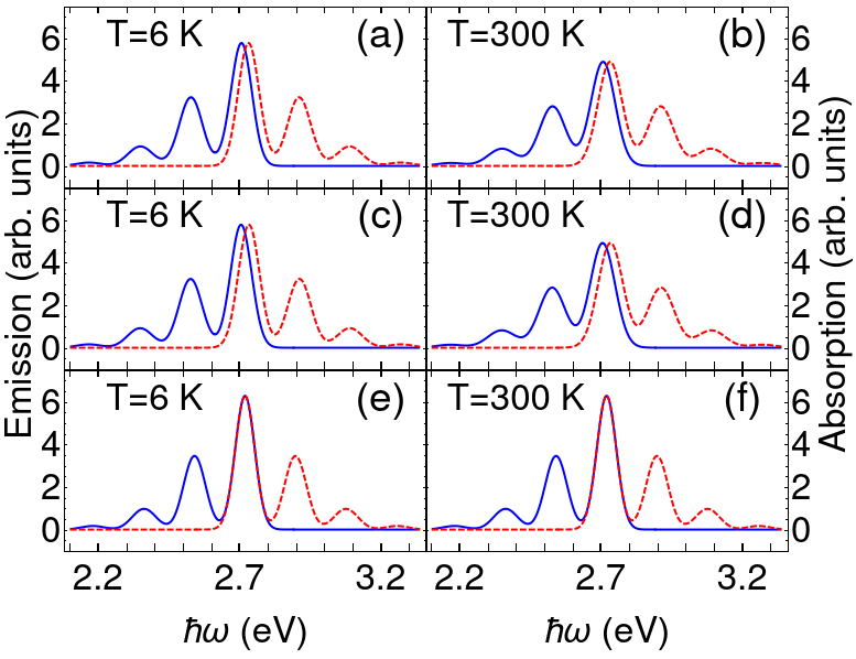
Figure 1: The emission (blue solid line) and absorption (red dashed line) spectra of a bare MeLPPP layer at different temperatures (a), (c), (e) $T=6~{}{\rm K}$; (b), (d), (f) $T=300~{}{\rm K}$. The spectra in (a) and (b) explicitly take into account all the vibrational modes according to exact expressions Eq. (34) and (35), the spectra (c) and (d) take into account low-frequency vibrational modes effectively according to Eq. (37) and (38), the spectra (e) and (f) utilize the exact model while neglecting low-frequency modes.

To extract polariton thermalization rate we proceed with the following steps. First, we calculate the emission and absorption spectra of the bare MeLPPP layer at different temperatures and extract the net properties of the low-frequency vibrations according to Eq. (27)–(28). Second, we use the extracted net values of $A_{1}$ and $A_{2}$ to estimate polariton thermalization rate Eq. (29) and (30) as the function of light-matter interaction (12) and the energy of the ground state of polaritons.

Our comparison of the emission and absorption spectra starts by employing three separate approaches: (i) the exact microscopic model as defined by Eq. (34)–(35); (ii) the reduced model accounting for the net effect of low-energy vibrational modes Eq. (37)–(38); and (iii) the exact model again, but this time excluding all low-energy modes. Figure 1 presents the results of these calculations at two different temperatures, 6K and 300K. Our reduced method agrees well on a quantitative level with the exact microscopic model that includes all mentioned vibrational modes. Furthermore, it is clear that neglecting low-energy modes fails to accurately reproduce the Stokes shift and linewidth in the spectra.

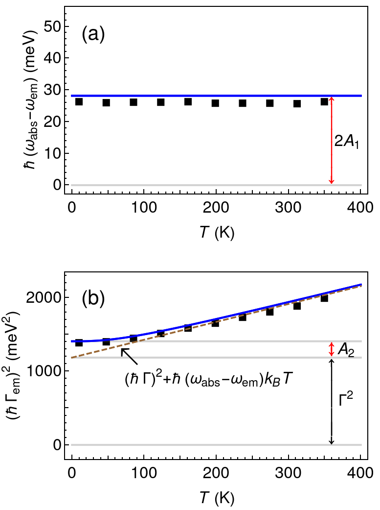
Figure 2: Temperature dependence of the Stokes shift - (a) and linewidth - (b) of $0-0$ emission peak. The dashed line shows the asymptotic behaviour of the linewidth at high temperatures. Red double arrows mark the net values of the low-frequency vibration, namely $A_{1}$ and $A_{2}$ parameters.

The comparison between our theoretical predictions and the experimental absorption and emission spectra reported in the literature demonstrates a quantitative match, including the observed slight asymmetry in the spectral lines [72, 73, 39]. It is important to note that our theory primarily accounts for the effects of low-energy vibrational (geometric) relaxation and does not take into account factors such as intermolecular interactions or spin multiplicity change. As a result, this theoretical approach is most effective for molecular systems that exhibit a pronounced mirroring of vibronic replicas in their spectra.

The Stokes shift and the linewidth of the 0-0 emission peak can be extracted from Figure 1(a,b). We have expanded this dataset with additional calculations using the exact model across a range of temperatures from 6K to 400K. Figure (2) shows the Stokes shift and the linewidth as the function of temperature. Importantly the results obtained from the reduced model using analytical expressions Eq. (39)–(40) are in good agreement with the exact method (Fig. 2) and experimental data [39]. Although the Stokes shift remains constant with temperature changes (Fig. 2a), the linewidth stays constant only at low temperatures and increases linearly with temperature, as illustrated in Fig. 2b. Finally, the joint analysis of the emission and absorption spectra at different temperatures allows us to determine the net values $A_{1}\approx 18~{}{\rm meV}$ and $A_{2}\approx 200~{}{\rm meV}^{2}$ of the low-frequency vibrations, defining polariton thermalization rates Eq. (29)–(30).

Next, we demonstrate how the net values $A_{1}$ and $A_{2}$, obtained from the spectral analysis of the bare MeLPPP layer, can be applied to calculate the polariton thermalization rate in practical microcavities [34, 24, 12]. We make use of the equation (30) to extract thermalization rates between neighbouring states in the momentum space, for example $\hbar\bf k^{\prime}=0$, and $\hbar\bf k=\hbar\bf k^{\prime}+\hbar\bf{\delta k}$, with the corresponding energy being $\hbar\omega_{{\rm low}{\bf k}}=\hbar\omega_{{\rm low}{\bf k^{\prime}}}+4\pi\alpha_{\rm pol}/S$, where $\alpha_{\rm pol}$ is the dispersion relation of the lower polariton branch according Eq. (17)

$$\alpha_{\rm pol}\approx\frac{\alpha_{\rm cav}}{2}\left[1+\frac{\omega_{0}-\omega_{{\rm cav}{\bf k}={\bf 0}}}{\sqrt{(\omega_{0}-\omega_{{\rm cav}{\bf k}={\bf 0}})^{2}+4\Omega_{R}^{2}}}\right].$$ (46)

As the cutoff frequency for low-energy vibrations we use ${\omega_{M}\approx 200~{}{\rm cm}^{-1}}$.

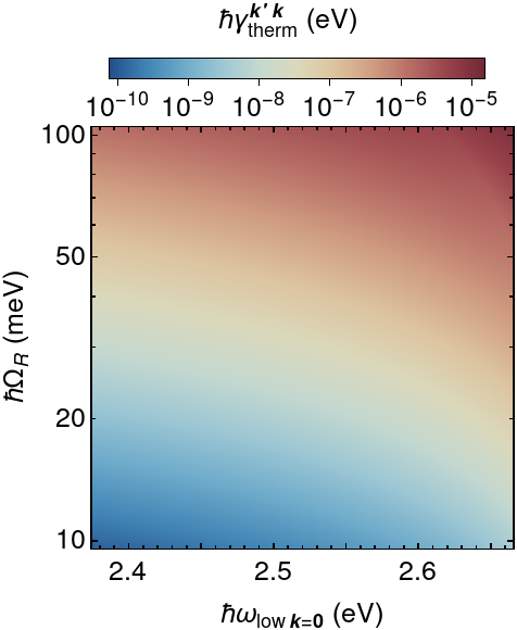
Figure 3: Polariton thermalization rate calculated from the spectral analysis according to Eq. (29) as the function of light-matter interaction strength (Rabi frequency $\Omega_{R}$) and the energy of the ground polariton state ($\hbar\omega_{{\rm low}{\bf k}={\bf 0}}$).

Figure 3 presents the extracted values of the polariton thermalization rate as the function of light-matter interaction (Rabi frequency $\Omega_{R}$) and the energy of the ground polariton state ($\omega_{{\rm low}{\bf k}={\bf 0}}$). It should be noted that the polariton thermalization rate has not been directly measured to date and has always been treated as a variable parameter in the fitting of experimental data by microscopic and/or mean-field models [74, 75, 76, 58, 12]. Here, we introduce an independent method that provides direct access to the thermalization rate in molecular polariton systems without relying on any adjustable parameters.

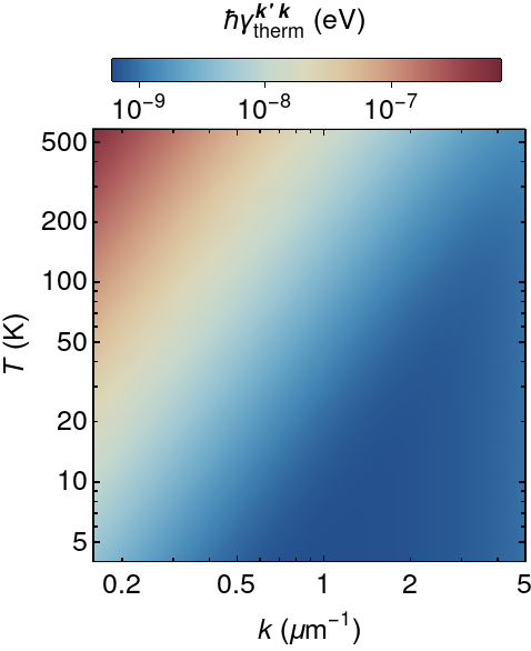
Figure 4: Temperature dependence of the polariton thermalization rate between the ground polariton state (${\bf k}^{\prime}={\bf 0}$) and the state with given wavevector $\bf k$ (hor. axis). Here we set $\hbar\omega_{{\rm cav}{\bf k}={\bf 0}}=2.53~{}{\rm eV}$ and $\hbar\Omega_{R}=55~{}{\rm meV}$. For the sake of consistency all the other parameters are taken the same as for Fig 3.

Even though thermalization processes reflect the matter behaviour in polariton states, the design of the cavity is expected to have a notable impact, especially regarding aspects tied to the Hopfield coefficients of light-matter states, such as exciton-cavity detuning and mode volume. The general rule of a thumb is that an increase in the material component of the polaritons results in a higher thermalization rate (Fig. 3). As depicted in Figure 3 the polariton thermalization rate monotonically increases with the Rabi frequency. Despite the explicit dependence on the number of molecules in Eq. (20)–(21) and Eq. (29)–(30), the thermalization rate does not decrease with the increase in $N_{\rm mol}$, because $\Omega_{R}\propto\sqrt{N_{\rm mol}}$. Moreover, the thermalization rate grows with the concentration of the molecules due to the growth of material component of the polaritons, which is described by the Hopfield coefficients in Eq. (20)–(21). This observation is in agreement with polartion plasmon systems [58].

Temperature is another cricual parameter in polariton thermalization. The thermalization rate given by Eq. (29)–(30) exhibits very strong dependence on temperature due to the factor $n_{\rm v}(\Delta\omega_{{\bf kk}^{\prime}})$. Figure 4 demonstrates the peculiar thermalization behavior. First, the temperature rise leads to an almost linear increase in the thermalization rate to the energetically closest polariton state. Secondly, at higher temperatures, the range of polariton states capable of effective thermalization to a specific state expands, or alternatively, it increases the thermalization length, defined as the number of states to which a polariton can efficiently thermalize. These results are in remarkable agreement with the recent experimental studies and emphasize the distinct role of thermalization proccesses in nonequilibrium Bose–Einstein condensation of molecular exciton-polaritons [12]. The developed formalism enable direct access to the value of polariton thermalization rate and provide rigorous elaboration for the thermalization bottleneck effect observed in organic microcavities at low temperatures [34].

VI Conclusion

In this work, we investigate the microscopic origins of polariton thermalization in organic systems. We have developed a theoretical framework that encompasses both strong light-matter and vibronic couplings. The main focus of our study is the role of low-energy vibrations in shaping the spectral properties of molecular systems and their interplay with polariton thermalization when strongly coupled to an optical cavity. Analytical expressions for emission and absorption spectra have been derived to effectively incorporate low-frequency vibrational coupling. We introduced net values accounting for the ensemble averaged properties of low-energy modes, which can be extracted directly from the Stokes shift ($A_{1}$) and the temperature-dependent linewidth of the 0-0 vibronic peak in the emission spectrum ($A_{2}$) of the molecular system without a cavity. In the next step, we established the correspondence between the spectral properties of the molecular system and the polariton thermalization within the cavity.

We have derived a simple analytical expression for the polariton thermalization rate that is proportional to the ratio $\sim(A_{1}^{2}/A_{2})$, meaning a high thermalization rate requires a large Stokes shift and should exhibit linear dependence on the spectral broadening with temperature, starting from low temperatures. Moreover, the polariton thermalization rate depends strongly on temperature and the cavity properties. Finally, we applied the developed formalism to a practical microcavity structure based on the MeLPPP conjugated polymer and calculated the thermalization rate without the use of any free parameters. Our results showcase remarkable agreement with recent experimental demonstrations of nonequilibrium polariton condensation in the ground [34, 24, 12] and excited [77] states, and explain the thermalization bottleneck effect at low temperatures [34].

Our research lays the groundwork for understanding nonequilibrium polariton condensation in molecular systems, its interplay with vibrational degrees of freedom, and serves as a guideline for future experimental studies, providing recipes to choose the right material system and cavity design, as well as conditions to control the thermalization behavior in strongly coupled molecular systems.

Appendix A Emission spectrum of an organic film

The stationary emission spectrum, $I_{\rm em}(\omega)$, can be calculated as follows [45, 49]

$$I_{\rm em}(\omega)=C_{\rm em}\sum_{m=1}^{N_{\rm mol}}{\rm Re}\int^{+\infty}_{0}e^{-i\omega\tau}\langle\hat{\sigma}^{(m){\dagger}}(t+\tau)\hat{\sigma}^{(m)}(t)\rangle d\tau$$ (47)

where $t\to\infty$ and $C_{\rm em}$ is the normalization constant. We set $C_{\rm em}$ such that

$$\int_{-\infty}^{+\infty}I_{\rm em}(\omega)d\omega=1.$$ (48)

We assume that the weak incoherent pumping supplies the energy to the dressed excitons and do not affect the dressed molecular vibrations. In this case, we can separate contribution of these two subsystems in the two-time correlator form Eq. (47)

$$\langle\hat{\sigma}^{(m){\dagger}}(t+\tau)\hat{\sigma}^{(m)}(t)\rangle\approx\langle\hat{S}^{(m){\dagger}}(t+\tau)\hat{S}^{(m)}(t)\rangle\prod_{j=1}^{N_{\rm vib}}\langle\hat{D}_{j}^{(m){\dagger}}(t+\tau)\hat{D}_{j}^{(m)}(t)\rangle,$$ (49)

The analysis of the dynamics of the excitons at $t\to+\infty$ leads to the following

$$\langle\hat{S}^{\dagger}(t+\tau)\hat{S}(t)\rangle=pe^{-(\gamma_{\rm diss}/2-i\omega_{0})\tau},$$ (50)

.

To obtain $\langle\hat{D}^{(m){\dagger}}_{j}(t+\tau)\hat{D}^{(m)}_{j}(t)\rangle$ at $t\to+\infty$, we consider the correlator

$${\langle\hat{R}^{(m)}_{j}(t+\tau,\mu_{1},\mu_{2})\hat{D}^{(m)}_{j}(t)\rangle},$$

where $\hat{R}^{(m)}_{j}(t+\tau,\mu_{1},\mu_{2})=e^{\mu_{1}\hat{B}^{(m){\dagger}}_{j}(t+\tau)}e^{-\mu_{2}\hat{B}^{(m)}_{j}(t+\tau)}$. Using the Lindblad equation (31) and the quantum regression theorem [45, 49], we obtain an equation for this correlator

$$\frac{\partial}{\partial\tau}\langle\hat{R}^{(m)}_{j}(t+\tau,\mu_{1},\mu_{2})\hat{D}^{(m)}_{j}(t)\rangle=\\ \left(-(\gamma_{{\rm v}j}-i\omega_{{\rm v}j})\mu_{1}\frac{\partial}{\partial\mu_{1}}-(\gamma_{{\rm v}j}+i\omega_{{\rm v}j})\mu_{2}\frac{\partial}{\partial\mu_{2}}-2\gamma_{{\rm v}j}n_{{\rm v}j}\mu_{1}\mu_{2}\right)\langle\hat{R}^{(m)}_{j}(t+\tau,\mu_{1},\mu_{2})\hat{D}^{(m)}_{j}(t)\rangle.$$ (51)

with the initial conditions

$$\langle\hat{R}^{(m)}_{j}(t,\mu_{1},\mu_{2})\hat{D}^{(m)}_{j}(t)\rangle=\langle e^{\mu_{1}\hat{B}^{(m){\dagger}}_{j}(t)}e^{-\mu_{2}\hat{B}^{(m)}_{j}(t)}e^{-\Lambda_{j}(\hat{B}_{j}^{(m){\dagger}}(t)-\hat{B}_{j}^{(m)})(t)}\rangle$$ (52)

One can show that

$$\langle\hat{R}^{(m)}_{j}(t,\mu_{1},\mu_{2})\hat{D}^{(m)}_{j}(t)\rangle=e^{-\Lambda_{j}^{2}/2}e^{\mu_{2}\Lambda_{j}}e^{-n_{{\rm v}j}(\Lambda_{j}-\mu_{1})(\Lambda_{j}-\mu_{2})}.$$ (53)

From here, we can find the solution to the equation (51)

$$\langle\hat{R}^{(m)}_{j}(t+\tau,\mu_{1},\mu_{2})\hat{D}^{(m)}_{j}(t)\rangle=e^{-\Lambda_{j}^{2}/2}e^{-n_{{\rm v}j}\Lambda_{j}^{2}}e^{-n_{{\rm v}j}\mu_{1}\mu_{2}}e^{n_{{\rm v}j}\Lambda_{j}\mu_{1}e^{-(\gamma_{{\rm v}j}-i\omega_{{\rm v}j})\tau}}e^{(1+n_{{\rm v}j})\Lambda_{j}\mu_{2}e^{-(\gamma_{{\rm v}j}+i\omega_{{\rm v}j})\tau}}.$$ (54)

Using equality $\langle\hat{D}^{(m){\dagger}}_{j}(t+\tau)\hat{D}^{(m)}_{j}(t)\rangle=e^{-\Lambda_{j}^{2}/2}\langle\hat{R}^{(m)}_{j}(t+\tau,\Lambda_{j},\Lambda_{j})\hat{D}^{(m)}_{j}(t)\rangle$, we finally obtain

$$\langle\hat{D}^{(m){\dagger}}_{j}(t+\tau)\hat{D}^{(m)}_{j}(t)\rangle=e^{-n_{{\rm v}j}\Lambda_{j}^{2}}e^{n_{{\rm v}j}\Lambda_{j}^{2}e^{-(\gamma_{{\rm v}j}-i\omega_{{\rm v}j})\tau}}e^{-(1+n_{{\rm v}j})\Lambda_{j}^{2}}e^{(1+n_{{\rm v}j})\Lambda_{j}^{2}e^{-(\gamma_{{\rm v}j}+i\omega_{{\rm v}j})\tau}}.$$ (55)

Substitution of Eq. (50) and Eq. (55) into Eq. (49) allows us to transform Eq. (47) into the following form:

$$I_{\rm em}(\omega)=\sum_{k^{\prime}_{1},...,k^{\prime}_{N_{\rm vib}}}z_{k^{\prime}_{1}}(n_{{\rm v}1}\Lambda_{1}^{2})...z_{k^{\prime}_{N_{\rm vib}}}(n_{{\rm v}N_{\rm vib}}\Lambda_{N_{\rm vib}}^{2})\\ \sum_{k_{1},...,k_{N_{\rm vib}}}z_{k_{1}}((1+n_{{\rm v}1})\Lambda_{1}^{2})...z_{k_{M}}((1+n_{{\rm v}N_{\rm vib}})\Lambda_{N_{\rm vib}}^{2})\\ \frac{1}{N_{\rm mol}}\sum_{m=1}^{N_{\rm mol}}\frac{\gamma_{\rm diss}/2+\gamma_{{\rm v}\Sigma}}{(\omega-\omega_{0}^{(m)}+\omega_{{\rm v}\Sigma})^{2}+(\gamma_{\rm diss}/2+\gamma_{{\rm v}\Sigma})^{2}},$$ (56)

where we introduced

$$\omega_{{\rm v}\Sigma}=\sum_{j=1}^{N_{\rm vib}}\omega_{{\rm v}j}(k_{j}-k^{\prime}_{j}),$$ (57)

$$\gamma_{{\rm v}\Sigma}=\sum_{j=1}^{N_{\rm vib}}\gamma_{{\rm v}j}(k_{j}+k^{\prime}_{j}).$$ (58)

Equation (56) at $T=0$ ($n_{{\rm v}j}=0$) coincides with the result in Ref. [7] obtained within Heisenberg–Langevin formalism.

The typical number of illuminated molecules in the organic molecular film is $10^{8}-10^{9}$. Therefore, the distribution of the exciton energies can be treated as continuous. We assume that it has normal distribution with the standard deviation $\Gamma$. We also assume that $\Gamma\gg\gamma_{\rm diss}/2+\gamma_{{\rm v}\Sigma}$. In this case, the inhomogeneous broadening leads to the Gaussian lineshapes of the spectral peaks [53, 55, 56, 57, 2]. Thus, from Eq. (56), we obtain Eq. (34).

To obtain Eq. (37) from Eq. (34), we change the sums in Eq. (34) corresponding to the low-frequency vibrations as follows

$$\sum_{n=0}^{+\infty}\frac{e^{-x}x^{n}}{n!}...=\left.\frac{2}{1+{\rm efr}\left(\sqrt{x/2}\right)}\frac{1}{\sqrt{2\pi x}}\int_{0}^{+\infty}dye^{-(y-x)^{2}/2x}...\right|_{n\to y}$$ (59)

Appendix B Absorption spectrum of an organic film

The absorption spectrum, $I_{\rm abs}(\omega)$, can be calculated according to the following equation [52]

$$I_{\rm abs}(\omega_{\Omega})=-C_{\rm abs}\sum_{m=1}^{N_{\rm mol}}{\rm Im}\langle\hat{\sigma}^{(m)}(t)e^{i\omega_{\Omega}t}\rangle/\Omega,$$ (60)

where ${t\to+\infty}$ and $C_{\rm abs}$ is the normalization constant. We set $C_{\rm abs}$ such that

$$\int_{-\infty}^{+\infty}I_{\rm abs}(\omega)d\omega=1.$$ (61)

In the basis of dressed states, the expression for the absorption spectrum has the form

$$I_{\rm abs}(\omega_{\Omega})=-\frac{C_{\rm abs}}{\Omega}\sum_{m=1}^{N_{\rm mol}}{\rm Im}\left\langle\prod_{j=1}^{N_{\rm vib}}\hat{D}_{j}^{(m)}(t)\hat{S}^{(m)}(t)e^{i\omega_{\Omega}t}\right\rangle$$ (62)

The Lindblad equation (31) allows us to write the Heisenberg-Langevin equation for the operator $\hat{S}(t)$

$$\frac{d}{dt}\hat{S}^{(m)}(t)=-(\gamma_{\rm diss}/2+i\omega_{0}^{(m)})\hat{S}^{(m)}(t)-i\Omega\hat{D}^{(m){\dagger}}(t)e^{-i\omega_{\Omega}t}+\hat{F}^{(m)}(t),$$ (63)

where $\hat{F}^{(m)}(t)$ is the noise acting on the dressed electronic state due to the interaction with the environment, while $\langle\hat{F}^{(m)}(t)\rangle=0$ (white noise). In the equation (63), we discarded the term that is nonlinear in $\hat{S}^{(m)}(t)$, assuming that the external field is weak.

We find the operator $\hat{S}(t)$ by integrating the equation (63), then we substitute the result into the expression for $I_{\rm abs}(\omega_{\Omega})$, and obtain

$$I_{\rm abs}(\omega_{\Omega})=C_{\rm abs}\sum_{m=1}^{N_{\rm mol}}{\rm Re}\int_{0}^{+\infty}\prod_{j=1}^{N_{\rm vib}}\left\langle\hat{D}_{j}^{(m)}(t)\hat{D}_{j}^{(m){\dagger}}(t^{\prime})\right\rangle e^{i\omega_{\Omega}(t-t^{\prime})}e^{-(\gamma_{\rm diss}/2+i\omega_{0})(t-t^{\prime})}dt^{\prime}.$$ (64)

Here, we assume that the noise acting on the dressed electronic state is uncorrelated with the dressed vibrational states of the molecule, i.e. $\langle\hat{D}_{j}^{(m)}(t)\hat{F}^{(m)}(t)\rangle=\langle\hat{D}_{j}^{(m)}(t)\rangle\langle\hat{F}^{(m)}(t)\rangle=0$.

The correlator ${\langle\hat{D}_{j}^{(m)}(t)\hat{D}_{j}^{(m){\dagger}}(t^{\prime})\rangle}$ can be obtained in the same way as we did it for $\langle\hat{D}_{j}^{(m){\dagger}}(t+\tau)\hat{D}_{j}^{(m)}(t)\rangle$ in Section A. Thus, we get absorption spectrum in the following form

$$I_{\rm abs}(\omega)=\sum_{k^{\prime}_{1},...,k^{\prime}_{N_{\rm vib}}}z_{k^{\prime}_{1}}(n_{{\rm v}1}\Lambda_{1}^{2})...z_{k^{\prime}_{N_{\rm vib}}}(n_{{\rm v}N_{\rm vib}}\Lambda_{N_{\rm vib}}^{2})\\ \sum_{k_{1},...,k_{N_{\rm vib}}}z_{k_{1}}((1+n_{{\rm v}1})\Lambda_{1}^{2})...z_{k_{M}}((1+n_{{\rm v}N_{\rm vib}})\Lambda_{N_{\rm vib}}^{2})\\ \frac{1}{N_{\rm mol}}\sum_{m=1}^{N_{\rm mol}}\frac{\gamma_{\rm diss}/2+\gamma_{{\rm v}\Sigma}}{(\omega-\omega_{0}^{(m)}-\omega_{{\rm v}\Sigma})^{2}+(\gamma_{\rm diss}/2+\gamma_{{\rm v}\Sigma})^{2}}.$$ (65)

At zero temperature ($n_{{\rm v}j}=0$) Eq. (65) coincides with the equation obtained in Ref.n [7].

As we did in the Section A we can take into account inhomogeneous broadening and obtain Eq. (35) from Eq. (65). Using Eq. (59), we can effectively incorporate low-frequency vibrational modes and obtain Eq. (38) from Eq. (35).

References

- Jang and Mennucci [2018] S. J. Jang and B. Mennucci, Delocalized excitons in natural light-harvesting complexes, Reviews of Modern Physics 90, 035003 (2018).
- Ostroverkhova [2016] O. Ostroverkhova, Organic optoelectronic materials: mechanisms and applications, Chemical reviews 116, 13279 (2016).
- Hadziioannou and Malliaras [2006] G. Hadziioannou and G. G. Malliaras, Semiconducting polymers: chemistry, physics and engineering (John Wiley & Sons, 2006).
- Martínez-Martínez and Arbeloa [2020] V. Martínez-Martínez and F. L. Arbeloa, Dyes and photoactive molecules in microporous systems (Springer, 2020).
- Gierschner et al. [2003] J. Gierschner, H.-G. Mack, H.-J. Egelhaaf, S. Schweizer, B. Doser, and D. Oelkrug, Optical spectra of oligothiophenes: vibronic states, torsional motions, and solvent shifts, Synthetic metals 138, 311 (2003).
- Kirton and Keeling [2015] P. Kirton and J. Keeling, Thermalization and breakdown of thermalization in photon condensates, Physical Review A 91, 033826 (2015).
- Reitz et al. [2019] M. Reitz, C. Sommer, and C. Genes, Langevin approach to quantum optics with molecules, Physical review letters 122, 203602 (2019).
- Brédas et al. [2004] J.-L. Brédas, D. Beljonne, V. Coropceanu, and J. Cornil, Charge-transfer and energy-transfer processes in -conjugated oligomers and polymers: a molecular picture, Chemical reviews 104, 4971 (2004).
- Coles et al. [2011] D. M. Coles, P. Michetti, C. Clark, W. C. Tsoi, A. M. Adawi, J.-S. Kim, and D. G. Lidzey, Vibrationally assisted polariton-relaxation processes in strongly coupled organic-semiconductor microcavities, Advanced Functional Materials 21, 3691 (2011).
- Hestand and Spano [2018] N. J. Hestand and F. C. Spano, Expanded theory of h-and j-molecular aggregates: the effects of vibronic coupling and intermolecular charge transfer, Chemical reviews 118, 7069 (2018).
- Kirton and Keeling [2013] P. Kirton and J. Keeling, Nonequilibrium model of photon condensation, Physical review letters 111, 100404 (2013).
- Zasedatelev et al. [2021] A. V. Zasedatelev, A. V. Baranikov, D. Sannikov, D. Urbonas, F. Scafirimuto, V. Y. Shishkov, E. S. Andrianov, Y. E. Lozovik, U. Scherf, T. Stöferle, et al., Single-photon nonlinearity at room temperature, Nature 597, 493 (2021).
- Shishkov et al. [2023] V. Y. Shishkov, E. S. Andrianov, S. Tretiak, K. B. Whaley, and A. V. Zasedatelev, Mapping polariton bose–einstein condensate onto vibrational degrees of freedom (2023), arXiv:2309.08498 [cond-mat.quant-gas] .
- Herrera and Spano [2017] F. Herrera and F. C. Spano, Dark vibronic polaritons and the spectroscopy of organic microcavities, Physical Review Letters 118, 223601 (2017).
- Rodriguez et al. [2013] S. Rodriguez, J. Feist, M. Verschuuren, F. G. Vidal, and J. G. Rivas, Thermalization and cooling of plasmon-exciton polaritons: towards quantum condensation, Physical review letters 111, 166802 (2013).
- Wu et al. [2016] N. Wu, J. Feist, and F. J. Garcia-Vidal, When polarons meet polaritons: Exciton-vibration interactions in organic molecules strongly coupled to confined light fields, Physical Review B 94, 195409 (2016).
- Deng et al. [2010] H. Deng, H. Haug, and Y. Yamamoto, Exciton-polariton bose-einstein condensation, Reviews of Modern Physics 82, 1489 (2010).
- Imamog et al. [1996] A. Imamog, R. Ram, S. Pau, Y. Yamamoto, et al., Nonequilibrium condensates and lasers without inversion: Exciton-polariton lasers, Physical Review A 53, 4250 (1996).
- Shishkov et al. [2022a] V. Y. Shishkov, E. S. Andrianov, A. V. Zasedatelev, P. G. Lagoudakis, and Y. E. Lozovik, Exact analytical solution for the density matrix of a nonequilibrium polariton bose-einstein condensate, Physical Review Letters 128, 065301 (2022a).
- Shishkov et al. [2022b] V. Y. Shishkov, E. Andrianov, and Y. E. Lozovik, Analytical framework for non-equilibrium phase transition to bose–einstein condensate, Quantum 6, 719 (2022b).
- Satapathy et al. [2022] S. Satapathy, B. Liu, P. Deshmukh, P. M. Molinaro, F. Dirnberger, M. Khatoniar, R. L. Koder, and V. M. Menon, Thermalization of fluorescent protein exciton–polaritons at room temperature, Advanced Materials 34, 2109107 (2022).
- Väkeväinen et al. [2020] A. I. Väkeväinen, A. J. Moilanen, M. Nečada, T. K. Hakala, K. S. Daskalakis, and P. Törmä, Sub-picosecond thermalization dynamics in condensation of strongly coupled lattice plasmons, Nature communications 11, 3139 (2020).
- Peng and Rabani [2023] K. Peng and E. Rabani, Polaritonic bottleneck in colloidal quantum dots, Nano Letters https://doi.org/10.1021/acs.nanolett.3c03508 (2023).
- Zasedatelev et al. [2019] A. V. Zasedatelev, A. V. Baranikov, D. Urbonas, F. Scafirimuto, U. Scherf, T. Stöferle, R. F. Mahrt, and P. G. Lagoudakis, A room-temperature organic polariton transistor, Nature Photonics 13, 378 (2019).
- Johnston et al. [2003] M. B. Johnston, L. M. Herz, A. L. Khan, A. Köhler, A. Davies, and E. Linfield, Low-energy vibrational modes in phenylene oligomers studied by thz time-domain spectroscopy, Chemical physics letters 377, 256 (2003).
- Shi et al. [2022] Y. Shi, Y. Chang, K. Lu, Z. Chen, J. Zhang, Y. Yan, D. Qiu, Y. Liu, M. A. Adil, W. Ma, et al., Small reorganization energy acceptors enable low energy losses in non-fullerene organic solar cells, Nature Communications 13, 3256 (2022).
- Bardeen et al. [1997] C. Bardeen, G. Cerullo, and C. Shank, Temperature-dependent electronic dephasing of molecules in polymers in the range 30 to 300 k, Chemical physics letters 280, 127 (1997).
- Karabunarliev et al. [2001] S. Karabunarliev, E. R. Bittner, and M. Baumgarten, Franck–condon spectra and electron-libration coupling in para-polyphenyls, The Journal of Chemical Physics 114, 5863 (2001).
- Beljonne et al. [2005] D. Beljonne, E. Hennebicq, C. Daniel, L. Herz, C. Silva, G. Scholes, F. Hoeben, P. Jonkheijm, A. Schenning, S. Meskers, et al., Excitation migration along oligophenylenevinylene-based chiral stacks: delocalization effects on transport dynamics, The Journal of Physical Chemistry B 109, 10594 (2005).
- Tretiak et al. [2002] S. Tretiak, A. Saxena, R. Martin, and A. Bishop, Conformational dynamics of photoexcited conjugated molecules, Physical review letters 89, 097402 (2002).
- Wiesenhofer et al. [2006] H. Wiesenhofer, E. Zojer, E. J. List, U. Scherf, J.-L. Brédas, and D. Beljonne, Molecular origin of the temperature-dependent energy migration in a rigid-rod ladder-phenylene molecular host, Advanced Materials 18, 310 (2006).
- Beenken and Pullerits [2004] W. J. Beenken and T. Pullerits, Spectroscopic units in conjugated polymers: a quantum chemically founded concept?, The Journal of Physical Chemistry B 108, 6164 (2004).
- Hennebicq et al. [2006] E. Hennebicq, C. Deleener, J.-L. Brédas, G. D. Scholes, and D. Beljonne, Chromophores in phenylenevinylene-based conjugated polymers: Role of conformational kinks and chemical defects, The Journal of chemical physics 125, https://doi.org/10.1063/1.2221310 (2006).
- Plumhof et al. [2014] J. D. Plumhof, T. Stöferle, L. Mai, U. Scherf, and R. F. Mahrt, Room-temperature bose–einstein condensation of cavity exciton–polaritons in a polymer, Nature materials 13, 247 (2014).
- Yamamoto et al. [2003] Y. Yamamoto, F. Tassone, and H. Cao, Semiconductor cavity quantum electrodynamics, Vol. 169 (Springer, 2003).
- Shishkov et al. [2019] V. Y. Shishkov, E. Andrianov, A. Pukhov, A. Vinogradov, and A. Lisyansky, Enhancement of the raman effect by infrared pumping, Physical review letters 122, 153905 (2019).
- Bässler and Schweitzer [1999] H. Bässler and B. Schweitzer, Site-selective fluorescence spectroscopy of conjugated polymers and oligomers, Accounts of Chemical Research 32, 173 (1999).
- Schindler et al. [2004] F. Schindler, J. M. Lupton, J. Feldmann, and U. Scherf, A universal picture of chromophores in -conjugated polymers derived from single-molecule spectroscopy, Proceedings of the National Academy of Sciences 101, 14695 (2004).
- Hoffmann et al. [2010] S. T. Hoffmann, H. Bässler, and A. Köhler, What determines inhomogeneous broadening of electronic transitions in conjugated polymers?, The Journal of Physical Chemistry B 114, 17037 (2010).
- Kahle et al. [2018] F.-J. Kahle, A. Rudnick, H. Bässler, and A. Köhler, How to interpret absorption and fluorescence spectra of charge transfer states in an organic solar cell, Materials Horizons 5, 837 (2018).
- Scafirimuto et al. [2021] F. Scafirimuto, D. Urbonas, M. A. Becker, U. Scherf, R. F. Mahrt, and T. Stöferle, Tunable exciton–polariton condensation in a two-dimensional lieb lattice at room temperature, Communications Physics 4, 39 (2021).
- Jiang et al. [2022] Z. Jiang, A. Ren, Y. Yan, J. Yao, and Y. S. Zhao, Exciton-polaritons and their bose–einstein condensates in organic semiconductor microcavities, Advanced Materials 34, 2106095 (2022).
- McGhee et al. [2021] K. E. McGhee, A. Putintsev, R. Jayaprakash, K. Georgiou, M. E. O’Kane, R. C. Kilbride, E. J. Cassella, M. Cavazzini, D. A. Sannikov, P. G. Lagoudakis, et al., Polariton condensation in an organic microcavity utilising a hybrid metal-dbr mirror, Scientific Reports 11, 20879 (2021).
- McGhee et al. [2022] K. E. McGhee, R. Jayaprakash, K. Georgiou, S. L. Burg, and D. G. Lidzey, Polariton condensation in a microcavity using a highly-stable molecular dye, Journal of Materials Chemistry C 10, 4187 (2022).
- Scully and Zubairy [1997] M. O. Scully and S. Zubairy, Quantum optics (CambridgeUniversity Press, Cambridge, England, 1997).
- Kavokin et al. [2017] A. V. Kavokin, J. J. Baumberg, G. Malpuech, and F. P. Laussy, Microcavities, Vol. 21 (Oxford university press, 2017).
- Breuer and Petruccione [2002] H.-P. Breuer and F. Petruccione, The theory of open quantum systems (Oxford University Press on Demand, 2002).
- Kubo [1957] R. Kubo, Statistical-mechanical theory of irreversible processes. i. general theory and simple applications to magnetic and conduction problems, Journal of the Physical Society of Japan 12, 570 (1957).
- Carmichael [2009] H. Carmichael, An open systems approach to quantum optics: lectures presented at the Université Libre de Bruxelles, October 28 to November 4, 1991, Vol. 18 (Springer Science & Business Media, 2009).
- Steiner et al. [2007] M. Steiner, A. Hartschuh, R. Korlacki, and A. J. Meixner, Highly efficient, tunable single photon source based on single molecules, Applied Physics Letters 90, 183122 (2007).
- Lombardi et al. [2020] P. Lombardi, M. Trapuzzano, M. Colautti, G. Margheri, I. P. Degiovanni, M. López, S. Kück, and C. Toninelli, A molecule-based single-photon source applied in quantum radiometry, Advanced Quantum Technologies 3, 1900083 (2020).
- Loudon [2000] R. Loudon, The quantum theory of light (OUP Oxford, 2000).
- Knapp [1984] E. Knapp, Lineshapes of molecular aggregates, exchange narrowing and intersite correlation, Chemical Physics 85, 73 (1984).
- Kador [1991] L. Kador, Stochastic theory of inhomogeneous spectroscopic line shapes reinvestigated, The Journal of chemical physics 95, 5574 (1991).
- Spano et al. [2009] F. C. Spano, J. Clark, C. Silva, and R. H. Friend, Determining exciton coherence from the photoluminescence spectral line shape in poly (3-hexylthiophene) thin films, The Journal of chemical physics 130 (2009).
- Guha et al. [2003] S. Guha, J. Rice, Y. Yau, C. M. Martin, M. Chandrasekhar, H. R. Chandrasekhar, R. Guentner, P. S. De Freitas, and U. Scherf, Temperature-dependent photoluminescence of organic semiconductors with varying backbone conformation, Physical Review B 67, 125204 (2003).
- Borrelli et al. [2014] R. Borrelli, S. Ellena, and C. Barolo, Theoretical and experimental determination of the absorption and emission spectra of a prototypical indolenine-based squaraine dye, Physical Chemistry Chemical Physics 16, 2390 (2014).
- Hakala et al. [2018] T. K. Hakala, A. J. Moilanen, A. I. Väkeväinen, R. Guo, J.-P. Martikainen, K. S. Daskalakis, H. T. Rekola, A. Julku, and P. Törmä, Bose–einstein condensation in a plasmonic lattice, Nature Physics 14, 739 (2018).
- Moilanen et al. [2021] A. J. Moilanen, K. S. Daskalakis, J. M. Taskinen, and P. Törmä, Spatial and temporal coherence in strongly coupled plasmonic bose-einstein condensates, Physical Review Letters 127, 255301 (2021).
- Johnson and Joannopoulos [2001] S. G. Johnson and J. D. Joannopoulos, Photonic crystals: the road from theory to practice (Springer Science & Business Media, 2001).
- Zhang et al. [2016] W. Zhang, J. Yao, and Y. S. Zhao, Organic micro/nanoscale lasers, Accounts of Chemical Research 49, 1691 (2016).
- Urbonas et al. [2016] D. Urbonas, T. Stöferle, F. Scafirimuto, U. Scherf, and R. F. Mahrt, Zero-dimensional organic exciton–polaritons in tunable coupled gaussian defect microcavities at room temperature, ACS Photonics 3, 1542 (2016).
- Scafirimuto et al. [2018] F. Scafirimuto, D. Urbonas, U. Scherf, R. F. Mahrt, and T. Stöferle, Room-temperature exciton-polariton condensation in a tunable zero-dimensional microcavity, ACS Photonics 5, 85 (2018).
- Zhu et al. [2016] W. Zhu, R. Esteban, A. G. Borisov, J. J. Baumberg, P. Nordlander, H. J. Lezec, J. Aizpurua, and K. B. Crozier, Quantum mechanical effects in plasmonic structures with subnanometre gaps, Nature communications 7, 11495 (2016).
- Benz et al. [2016] F. Benz, M. K. Schmidt, A. Dreismann, R. Chikkaraddy, Y. Zhang, A. Demetriadou, C. Carnegie, H. Ohadi, B. De Nijs, R. Esteban, et al., Single-molecule optomechanics in “picocavities”, Science 354, 726 (2016).
- Wersall et al. [2017] M. Wersall, J. Cuadra, T. J. Antosiewicz, S. Balci, and T. Shegai, Observation of mode splitting in photoluminescence of individual plasmonic nanoparticles strongly coupled to molecular excitons, Nano letters 17, 551 (2017).
- Baranov et al. [2018] D. G. Baranov, M. Wersall, J. Cuadra, T. J. Antosiewicz, and T. Shegai, Novel nanostructures and materials for strong light–matter interactions, Acs Photonics 5, 24 (2018).
- Xia et al. [2023] Y. Xia, M. Yamaguchi, and T.-Y. Luh, Ladder Polymers: Synthesis, Properties, Applications and Perspectives (John Wiley & Sons, 2023).
- Snedden et al. [2009] E. Snedden, R. Thompson, S. Hintshich, and A. Monkman, Fluorescence vibronic analysis in a ladder-type conjugated polymer, Chemical Physics Letters 472, 80 (2009).
- Hildner et al. [2009] R. Hildner, L. Winterling, U. Lemmer, U. Scherf, and J. Köhler, Single-molecule spectroscopy on a ladder-type conjugated polymer: Electron–phonon coupling and spectral diffusion, ChemPhysChem 10, 2524 (2009).
- Baderschneider et al. [2016] S. Baderschneider, U. Scherf, J. Köhler, and R. Hildner, Influence of the conjugation length on the optical spectra of single ladder-type (p-phenylene) dimers and polymers, The Journal of Physical Chemistry A 120, 233 (2016).
- Stampfl et al. [1995] J. Stampfl, W. Graupner, G. Leising, and U. Scherf, Photoluminescence and uv-vis absorption study of poly (para-phenylene)-type ladder-polymers, Journal of luminescence 63, 117 (1995).
- Pauck et al. [1996] T. Pauck, H. Bässler, J. Grimme, U. Scherf, and K. Müllen, A comparative site-selective fluorescence study of ladder-type para-phenylene oligomers and oligo-phenylenevinylenes, Chemical physics 210, 219 (1996).
- Deng et al. [2006] H. Deng, D. Press, S. Götzinger, G. S. Solomon, R. Hey, K. H. Ploog, and Y. Yamamoto, Quantum degenerate exciton-polaritons in thermal equilibrium, Physical review letters 97, 146402 (2006).
- Mazza et al. [2013] L. Mazza, S. Kéna-Cohen, P. Michetti, and G. C. La Rocca, Microscopic theory of polariton lasing via vibronically assisted scattering, Physical Review B 88, 075321 (2013).
- Daskalakis et al. [2014] K. Daskalakis, S. Maier, R. Murray, and S. Kéna-Cohen, Nonlinear interactions in an organic polariton condensate, Nature materials 13, 271 (2014).
- Baranikov et al. [2020] A. V. Baranikov, A. V. Zasedatelev, D. Urbonas, F. Scafirimuto, U. Scherf, T. Stöferle, R. F. Mahrt, and P. G. Lagoudakis, All-optical cascadable universal logic gate with sub-picosecond operation, arXiv preprint arXiv:2005.04802 https://doi.org/10.48550/arXiv.2005.04802 (2020).