Near-Field Velocity Sensing and Predictive Beamforming

Abstract

The novel concept of near-field velocity sensing is proposed. In contrast to far-field velocity sensing, near-field velocity sensing enables the simultaneous estimation of both radial and transverse velocities of a moving target. A maximum-likelihood-based method is proposed for jointly estimating the radial and transverse velocities from the echo signals. Assisted by near-field velocity sensing, a predictive beamforming framework is proposed for a moving communication user, which requires no channel estimation but achieves seamless data transmission. Finally, numerical examples validate the proposed approaches.

I Introduction

Recently, the near-field region of antenna arrays has garnered attention for its expanding influence with growing array aperture sizes and carrier frequencies [1, 2, 3, 4, 5]. Despite the complexity introduced by spherical-wave propagation in the near-field region, it opens new opportunities for both wireless communication and sensing. Specifically, near-field communication can enhance signal multiplexing through beamfocusing and degrees-of-freedom enhancement [1, 2]. Furthermore, near-field sensing allows simultaneous direction and distance estimation without requiring wideband resources or multiple sensing nodes required in far-field systems [3, 4, 5].

Against the above background, we further explore the potential of near-field propagation in wireless systems and propose the novel concept of near-field velocity sensing. Generally, the velocity of the target is estimated based on the Doppler frequency encapsulated in echo signals reflected by the target. In the far-field region, the Doppler frequency is only caused by the radial velocity of the target, which makes it difficult to estimate the transverse velocity of the target. Therefore, prior knowledge of the target motion model is generally required to obtain the full motion status of the target [6]. In this letter, we reveal that the Doppler frequency in the near-field is influenced by both radial and transverse velocities, which enables full motion status estimation of the target. To this end, we propose a maximum-likelihood-based near-field velocity sensing method. By leveraging near-field velocity sensing, we further propose a predictive beamforming approach for communication, which eliminates the requirements of channel estimation and facilitates seamless data transmission. Finally, numerical results are provided to validate the effectiveness of the proposed designs. The code is available at: https://github.com/zhaolin820/near-field-velocity-sensing-and-predictive-beamforming

II Near-Field Velocity Sensing

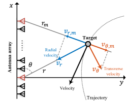
Figure 1: Illustration of the near-field velocity sensing.

II-A System Model

As shown in Fig. 1, we consider a narrowband near-field sensing system, which consists of a base station (BS) and a point-like moving target. The bandwidth of this system is denoted by $B$, which corresponds to a symbol duration $T_{s}=1/B$. The BS is equipped with an $M$-antenna uniform linear array (ULA) with spacing $d$. The ULA at the BS is deployed along the $x$-axis and the origin of the coordinate system is put into the center of the ULA. Then, the coordinate of the $m$-th antenna at the BS is given by $(\delta_{m}d,0)$, where $\delta_{m}=m-1-\frac{M-1}{2}$. Let $N$ denote the number of symbol durations for one coherent processing interval (CPI) for near-field sensing, during which the location and the velocity of the target remain constant. In a specific CPI, let $r$ and $\theta$ denote the distance and angle of the target with respect to the center of the ULA, respectively, and $v_{r}$ and $v_{\theta}$ denote the radial velocity and transverse velocity of the target with respect to the center of the ULA, respectively. As such, the coordinate of the target in this CPI is given by $(r\cos\theta,r\sin\theta)$. Let $\mathbf{s}(n)=[s_{1}(n),\dots,s_{M}(n)]\in\mathbb{C}^{M\times 1}$ denote the transmit signal of the BS at time index $n$, with $s_{m}(n)$ representing the transmit signal of the $m$-th antenna. An average power constraint should be satisfied by $\mathbf{s}(n)$, which is given by $\mathbb{E}[\mathbf{s}^{H}(n)\mathbf{s}(n)]=P_{t}$, with $P_{t}$ representing the transmit power. The received baseband echo signal at the $m$-th antenna, reflected by the moving target, is given by [7, 8]

$$y_{m}(n)=\sum_{i=1}^{M}\beta_{mi}e^{-j\frac{2\pi}{\lambda}(\bar{r}_{m}(nT_{s})+\bar{r}_{i}(nT_{s}))}s_{i}(n)+z_{m}(n),\vspace{-0.15cm}$$ (1)

where $\beta_{mi}$ denotes the channel gain, $\bar{r}_{m}(t)$ denotes the time-variant propagation distance from the $m$-th antenna to the target, $\lambda$ denotes the signal wavelength, and $z_{m}(n)\sim\mathcal{CN}(0,\sigma^{2})$ denotes the complex Gaussian noise. In particular, $\bar{r}_{m}(t)$ can be modeled as $\bar{r}_{m}(t)=r_{m}+v_{m}t$, where $r_{m}$ denotes the distance between the $m$-th antenna at the BS and the target and $v_{m}$ denotes the velocity component of the target projected along the line connecting the $m$-th antenna at the BS and the target. Based on the geometry relationship illustrated in Fig. 1, $r_{m}$ and $v_{m}$ can be expressed as

$$r_{m}=\sqrt{r^{2}+\delta_{m}^{2}d^{2}-2r\delta_{m}d\cos\theta},\quad v_{m}=v_{r,m}+v_{\theta,m},$$ (2)

where $v_{r,m}$ and $v_{\theta,m}$ are the projections of the radial velocity and the transverse velocity along the line connecting the $m$-th antenna and the target, respectively, and are given by

$$v_{r,m} =\frac{r-\delta_{m}d\cos\theta}{r_{m}}v_{r}=q_{m}v_{r},$$ (3)

$$v_{\theta,m} =\frac{\delta_{m}d\sin\theta}{r_{m}}v_{\theta}=p_{m}v_{\theta}.$$ (4)

Following the radar range equation [8], the channel gain $\beta_{mi}$ can be modeled as $\beta_{mi}=\frac{\beta}{r_{m}r_{i}}$. Here, $\beta$ is a constant satisfying $|\beta|^{2}=\frac{G_{t}G_{r}\lambda^{2}\sigma_{\text{RCS}}}{(4\pi)^{3}}$, where $G_{t}$ and $G_{r}$ denote the transmit and receive antenna gain, respectively, and $\sigma_{\text{RCS}}$ denotes the radar cross section. The overall received echo signal $\mathbf{y}(n)=[y_{1}(n),\dots,y_{M}(n)]^{T}$ can be expressed as

$$\mathbf{y}(n)= \beta\left(\mathbf{A}(r,\theta)\odot\mathbf{D}_{n}(v_{r},v_{\theta})\right)\mathbf{s}(n)+\mathbf{z}(n),\vspace{-0.15cm}$$ (5)

where $\odot$ is the Hadamard product, $\mathbf{A}(r,\theta)=\mathbf{a}(r,\theta)\mathbf{a}^{T}(r,\theta)$ with $\mathbf{a}(r,\theta)=[\frac{1}{r_{1}}e^{-j\frac{2\pi}{\lambda}r_{1}},\dots,\frac{1}{r_{M}}e^{-j\frac{2\pi}{\lambda}r_{M}}]^{T}$ denoting the array response vector, $\mathbf{D}_{n}(v_{r},v_{\theta})=\mathbf{d}_{n}(v_{r},v_{\theta})\mathbf{d}^{T}(v_{r},v_{\theta})$ with $\mathbf{d}_{n}(v_{r},v_{\theta})=[e^{-j\frac{2\pi}{\lambda}v_{1}nT_{s}},\dots,e^{-j\frac{2\pi}{\lambda}v_{M}nT_{s}}]^{T}$ denoting the Doppler-frequency vector, and $\mathbf{z}(n)$ is the noise vector.

II-B Velocity Sensing

Assuming that $\beta$, $r$, and $\theta$ have already been estimated, the vector containing the remaining unknown parameters is defined as $\boldsymbol{v}=[v_{r},v_{\theta}]^{T}$. By defining $\boldsymbol{\eta}=[r,\theta]^{T}$ and $\mathbf{H}_{n}(\boldsymbol{\eta},\boldsymbol{v})=\mathbf{A}(r,\theta)\odot\mathbf{D}_{n}(v_{r},v_{\theta})$, the echo signal received over one CPI can be expressed as

$$\mathbf{Y}=\big{[}\mathbf{y}(1),\mathbf{y}(2),\dots,\mathbf{y}(N)\big{]}=\beta\mathbf{X}(\boldsymbol{\eta},\boldsymbol{v})+\mathbf{Z},\vspace{-0.05cm}$$ (6)

where $\mathbf{X}(\boldsymbol{\eta},\boldsymbol{v})=[\mathbf{H}_{1}(\boldsymbol{\eta},\boldsymbol{v})\mathbf{s}(1),\dots,\mathbf{H}_{N}(\boldsymbol{\eta},\boldsymbol{v})\mathbf{s}(N)]$ and $\mathbf{Z}=[\mathbf{z}(1),\mathbf{z}(2),\dots,\mathbf{z}(N)]$. The unknown parameter $\boldsymbol{v}$ can be estimated by maximizing the likelihood, which can formulated as the following optimization problem:

$$\hat{\boldsymbol{v}}=\arg\min_{\boldsymbol{v}}\left\|\mathbf{Y}-\beta\mathbf{X}(\boldsymbol{\eta},\boldsymbol{v})\right\|_{F}^{2}=\arg\max_{\boldsymbol{v}}g(\mathbf{Y},\boldsymbol{\eta},\boldsymbol{v}),\vspace{-0.1cm}$$ (7)

where $\hat{\boldsymbol{v}}=[\hat{v}_{r},\hat{v}_{\theta}]^{T}$ denotes the estimated parameter and $g(\mathbf{Y},\boldsymbol{\eta},\boldsymbol{v})$ is given by

$$g(\mathbf{Y},\boldsymbol{\eta},\boldsymbol{v})=2\mathrm{Re} \left\{\mathrm{tr}\left(\beta\mathbf{X}(\boldsymbol{\eta},\boldsymbol{v})\mathbf{Y}^{H}\right)\right\}$$

$$-|\beta|^{2}\mathrm{tr}\left(\mathbf{X}(\boldsymbol{\eta},\boldsymbol{v})\mathbf{X}^{H}(\boldsymbol{\eta},\boldsymbol{v})\right).$$ (8)

The above problem is an unconstrained optimization problem. Thus, it can be solved by the classical gradient-based methods such as the gradient descent method and the quasi-Newton method, which generally require the gradient of the function $g(\mathbf{Y},\boldsymbol{\eta},\boldsymbol{v})$ with respect to the vector $\boldsymbol{v}$. According to the chain rule for complex numbers, the gradient $\frac{\partial g(\mathbf{Y},\boldsymbol{\eta},\boldsymbol{v})}{\partial v_{i}},\forall i\in\{r,\theta\},$ can be expressed as follows [9]:

$$\frac{\partial g(\mathbf{Y},\boldsymbol{\eta},\boldsymbol{v})}{\partial v_{i}}=2\mathrm{Re}\left\{\mathrm{tr}\left(\frac{\partial g(\mathbf{Y},\boldsymbol{\eta},\boldsymbol{v})}{\partial\mathbf{X}^{T}(\boldsymbol{\eta},\boldsymbol{v})}\frac{\partial\mathbf{X}(\boldsymbol{\eta},\boldsymbol{v})}{\partial v_{i}}\right)\right\}.\vspace{-0.1cm}$$ (9)

Then, we have

$$\frac{\partial g(\mathbf{Y},\boldsymbol{\eta},\boldsymbol{v})}{\partial\mathbf{X}^{T}(\boldsymbol{\eta},\boldsymbol{v})}=\beta\mathbf{Y}^{H}-|\beta|^{2}\mathbf{X}^{H}(\boldsymbol{\eta},\boldsymbol{v}).$$ (10)

Now, the remaining step is to calculate the partial derivatives $\frac{\partial\mathbf{X}(\boldsymbol{\eta},\boldsymbol{v})}{\partial v_{i}}=\left[\frac{\partial\mathbf{H}_{1}(\boldsymbol{\eta},\boldsymbol{v})}{\partial v_{i}}\mathbf{s}(1),\dots,\frac{\partial\mathbf{H}_{N}(\boldsymbol{\eta},\boldsymbol{v})}{\partial v_{i}}\mathbf{s}(N)\right]$. The expression of $\frac{\partial\mathbf{H}_{n}(\boldsymbol{\eta},\boldsymbol{v})}{\partial v_{i}}$ is derived as follows:

$$\frac{\partial\mathbf{H}_{n}(\boldsymbol{\eta},\boldsymbol{v})}{\partial v_{i}}=2\mathbf{A}(r,\theta)\odot\left(\frac{\partial\mathbf{d}_{n}(v_{r},v_{\theta})}{\partial v_{i}}\mathbf{d}_{n}^{T}(v_{r},v_{\theta})\right).$$ (11)

The partial derivative $\frac{\partial\mathbf{d}_{n}(v_{r},v_{\theta})}{\partial v_{i}}$ is given by

$$\frac{\partial\mathbf{d}_{n}}{\partial v_{i}}=-j\frac{2\pi}{\lambda}nT_{s}\left[d_{n,1}\frac{\partial v_{1}}{\partial v_{i}},\dots,d_{n,M}\frac{\partial v_{M}}{\partial v_{i}}\right]^{T},$$ (12)

where $d_{n,m}$ denotes the $m$-th entry of $\mathbf{d}_{n}(v_{r},v_{\theta})$. It can be readily obtained that $\frac{\partial v_{m}}{\partial v_{r}}=q_{m}$ and $\frac{\partial v_{m}}{\partial v_{t}}=p_{m}$.

Combining (9)-(12), the closed form gradient of function $g(\mathbf{Y},\boldsymbol{\eta},\boldsymbol{v})$ with respect to the vector $\boldsymbol{v}$ can be obtained. Based on this gradient, the gradient-based methods for solving problem (7) can be implemented using the existing toolbox, such as the function $\mathtt{fminunc}$ in the optimization toolbox of MATLAB [10]. The performance of these methods can be sensitive to the initialization point. Considering the fact that the location and the velocity of the target are not changed significantly between the adjacent CPIs, the initialization point can be selected based on previous CPI estimation to ensure performance, as elaborated in the following section.

Remark 1.

(Benefits of Near-Field Velocity Sensing) In far-field velocity sensing, since the links between each antenna and the sensing target are approximated to have the same direction, only the radial velocity of the target can be estimated. This fact is further underscored by expressions (3) and (4), where $q_{m}\rightarrow 1$ and $p_{m}\rightarrow 0$ as the distance $r$ becomes sufficiently large. However, within the near-field region where $p_{m}$ holds a non-negligible value, the simultaneous estimation of both radial and transverse velocities becomes achievable. In this case, the instantaneous motion status of the target can be obtained without the prior knowledge of the target motion model required in far-field regimes [6].

III Predictive Beamforming Through Near-Field Velocity Sensing

In this section, we explore using near-field velocity sensing in predictive beamforming for near-field communications. Typically, beamforming relies on channel state information influenced by the user’s location, necessitating channel estimation before data transmission in each CPI. Despite existing low-complexity methods, the pilot overhead remains high due to near-field channels requiring both distance and angular information between transceivers. To tackle this, we propose leveraging near-field velocity sensing for user tracking, enabling direct retrieval of the user’s current location based on prior sensing results. This approach allows for pilot-free and seamless predictive beamforming.

III-A Proposed Predictive Beamforming Framework

The proposed framework consists of the following steps.

• Initial Access: Upon the entry of a mobile user into the coverage area of the BS, the BS transmits isotropic beams in the first CPI to obtain the initial status of the moving users. In particular, the initial user location, user velocities, and the parameter $\beta$ can be estimated through a joint maximum likelihood method, similar to the process detailed in Section II-B, thus omitted here. These results serve as the initial input of the proposed framework and facilitate the design of beamforming in the second CPI.

• Data Transmission and Velocity Sensing: Leveraging the previously designed beamforming and the estimated user location in the previous CPI, the data can be effectively transmitted to the user and the radial and transverse velocities of the user in the current CPI can be estimated from the echo signals.

• Beam Prediction: Given estimated velocities, the user location in the next CPI can be predicted, which is then used to design the beamforming in the next CPI.

By repeating the second and third steps, pilot-free and seamless communication between the BS and a mobile user can be achieved in the near-field region. Next, we will elaborate on the communication model and the beam prediction method.

III-B Communication with Predictive Beamforming

Let $r_{l}$, $\theta_{l}$, $v_{r,l}$, and $v_{\theta,l}$ denote the distance, angle, radial velocity, and transverse velocity of the user in the $l$-th CPI, respectively. Then, under perfect synchronization, the user receives the following signal at time $n$ of the $l$-th CPI:

$$y_{c,l}(n)=\mathbf{h}_{l}^{H}(n)\mathbf{s}_{l}(n)+z_{c,l}(n),\vspace{-0.1cm}$$ (13)

where $\mathbf{h}_{l}^{H}(n)=\beta_{c}\mathbf{a}^{T}(r_{l},\theta_{l})\mathrm{diag}\left(\mathbf{d}_{n}(v_{r,l},v_{\theta,l})\right)\in\mathbb{C}^{1\times M}$ denotes the communication channel, $\beta_{c}$ is a constant containing antenna gain and carrier frequency, $\mathbf{s}_{l}(n)\in\mathbb{C}^{M\times 1}$ denotes the transmit signal satisfying $\mathbb{E}[\mathbf{s}_{l}^{H}(n)\mathbf{s}_{l}(n)]=P_{t}$ and $z_{c,l}(n)\sim\mathcal{CN}(0,\sigma^{2})$ denotes the complex Gaussian noise. Let $\hat{\boldsymbol{v}}_{l}=[\hat{v}_{r,l},\hat{v}_{\theta,l}]^{T}$ and $\hat{\boldsymbol{\eta}}_{l+1}=[\hat{r}_{l+1},\hat{\theta}_{l+1}]^{T}$ denote the estimated velocity vector and the predicted user location vector in the $l$-th CPI, respectively. In particular, the velocity vector $\hat{\boldsymbol{v}}_{l}$ can be estimated using maximum likelihood method proposed in Section II-B based on the predicted location $\hat{\boldsymbol{\eta}}_{l}$ in the $(l-1)$-th CPI, which is given by

$$\hat{\boldsymbol{v}}_{l}=\arg\max_{\boldsymbol{v}_{l}}g(\mathbf{Y}_{l},\hat{\boldsymbol{\eta}}_{l},\boldsymbol{v}_{l}),$$ (14)

where $\mathbf{Y}_{l}$ denotes the overall echo signal received at the BS in the $l$-th CPI. With $\hat{\boldsymbol{v}}_{l}$ at hand, the entries of $\hat{\boldsymbol{\eta}}_{l+1}$ can be calculated based on the physical relationship as follows:

$$\hat{r}_{l+1}=\hat{r}_{l}+\hat{v}_{r,l}NT_{s},\quad\hat{\theta}_{l+1}=\hat{\theta}_{l}+\frac{\hat{v}_{\theta,l}NT_{s}}{\hat{r}_{l}},$$ (15)

where $NT_{s}$ denotes the duration of a CPI. After obtaining $\hat{\boldsymbol{v}}_{l}$ and $\hat{\boldsymbol{\eta}}_{l+1}$, the beamforming in the $(l+1)$-th CPI can be designed to maximize the communication rate. Two key factors should be considered for this objective: array gain maximization and Doppler-frequency compensation. Specifically, maximizing array gain required the knowledge of user location, which has been estimated through (15). To compensate for the Doppler shift, the velocity information of the user is needed. Considering that the acceleration of typical mobile users (e.g., passenger vehicles), is generally small, it is safe to use the velocity estimated in the previous CPI to compensate for the Doppler shift. For example, let us consider a vehicle with an acceleration of $10\text{ m/s}^{2}$. The change of its velocity after a CPI of $0.02$ s is only $0.2$ m/s. Therefore, the transmit signal at time $n$ of the $(l+1)$-th CPI can be designed as

$$\mathbf{s}_{l+1}(n)=\mathbf{w}_{l+1}(n)c_{l+1}(n),\vspace{-0.1cm}$$ (16)

where $\mathbf{w}_{l+1}(n)=\sqrt{\rho}\mathrm{diag}(\mathbf{d}_{n}^{*}(\hat{v}_{r,l},\hat{v}_{\theta,l}))\mathbf{a}^{*}(\hat{r}_{l+1},\hat{\theta}_{l+1})\in\mathbb{C}^{M\times 1}$ denotes the predictive beamformer for the $(l+1)$-th CPI based on the sensing results obtained in the $l$-th CPI, $c_{l+1}(n)\in\mathbb{C}$ denotes the data symbol that can be modeled as an independent random variable with zero mean and unit power, and $\rho=P_{t}/M$ denotes the power regularization factor. Then, the average achievable rate over the $l$-th CPI is given by $R_{l}=\frac{1}{N}\sum_{n=1}^{N}\log\left(1+\frac{1}{\sigma^{2}}|\mathbf{h}_{l}^{H}(n)\mathbf{w}_{l}(n)|^{2}\right)$ [7].

IV Numerical Examples

In this section, numerical examples are provided to validate the feasibility of near-field velocity sensing and the effectiveness of the proposed predictive beamforming framework. Here, the BS is assumed to be equipped with $M=512$ antennas with $\lambda/2$ spacing. The carrier frequency is set to $28$ GHz. The system bandwidth and the length of a CPI are set to $B=100$ KHz and $2$ ms, respectively. Thus, we have $T_{s}=10^{-5}$ s and $N=200$. For the sensing channel, we set $G_{t}=G_{r}=1$ and $\sigma_{\text{RCS}}=1$. The noise density power is set to $-174$ dBm/Hz.

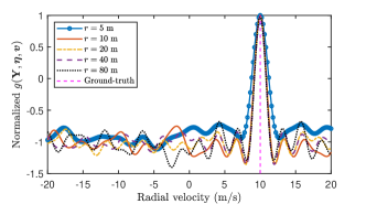
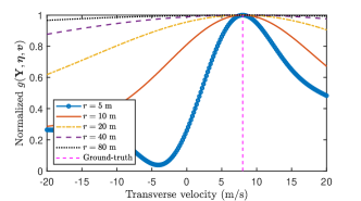
Figure 2: Performance of near-field velocity sensing.

In Fig. 2, the performance of the near-field velocity sensing is demonstrated for moving targets at different distances from the BS. The radial and transverse velocities of the targets are set to $v_{r}=10$ m/s and $v_{\theta}=8$ m/s, respectively. Other parameters of the target are assumed to be perfectly matched with the ground truth. For a fair comparison, the transmit power is adjusted according to the distance such that the signal-to-noise ratio remains the same. As can be observed from Fig. 2(a), function $g(\mathbf{Y},\boldsymbol{\eta},\boldsymbol{v})$ demonstrates a main lobe in close proximity to the ground truth, regardless of whether the target is near or far. It is also interesting to see that the main lobe becomes slightly narrower, which indicates improved performance in radial velocity sensing, as the target moves toward the far-field region. This phenomenon arises because, with increasing distance, the radial velocity manifested in the echo signal at each antenna gradually becomes the same, which is preferred by the radial velocity sensing. Concerning transverse velocity sensing, as illustrated in Fig. 2(b), it is notable that the function $g(\mathbf{Y},\boldsymbol{\eta},\boldsymbol{v})$ also has a main lobe in proximity to the ground truth. However, this main lobe progressively diminishes as the distance $r$ increases. At a distance of $r=80$ m, the function $g(\mathbf{Y},\boldsymbol{\eta},\boldsymbol{v})$ flattens over a substantial interval around the ground truth, rendering transverse velocity sensing impractical. These results are consistent with Remark 1.

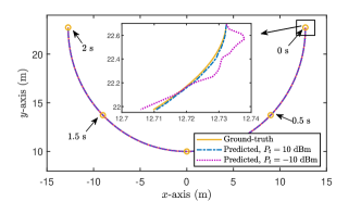
Figure 3: Predicted trajectory of the moving user.

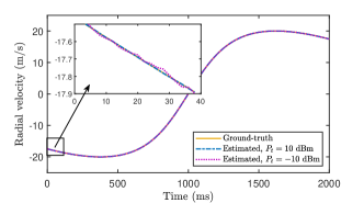
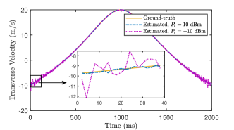
Figure 4: Estimated velocities of the moving user at different times.

Next, we study the performance of the proposed predictive beamforming scheme. Without loss of generality, we consider a moving user following the trajectory depicted in Fig. 3 at a speed of $20$ m/s, with the BS fixed at the origin of the coordinate system. The initial user location and parameter $\beta$ are assumed to be perfectly estimated at the initial access stage. The predicted trajectories, obtained through the proposed scheme at varying transmit powers, are also visualized in Fig. 3. Notably, the predicted trajectories closely align with the ground truth owning to the new velocity sensing ability in the near-field region. To gain more insights, Fig. 4 presents the estimated radial and transverse velocities of the moving user at each CPI, both of which closely match the ground-truth values, while transverse velocity sensing is more sensitive to user-BS distance compared to radial sensing. Furthermore, the robust performance of the proposed method is evident as it relies on predicted rather than ground-truth user locations, confirming its resilience against uncertainties.

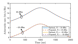
Figure 5: Achievable rate through predictive beamforming.

Finally, Fig. 5 illustrates the achievable rate $R_{l}$ attained through the proposed predictive beamforming scheme. In this context, the optimal achievable rate is determined by utilizing the ground-truth velocities and locations during the beamforming design. The results demonstrate that the proposed predictive beamforming achieves a performance closely approaching the optimal, which indicates that the proposed scheme can effectively maximize the array gain and compensate for the Doppler frequency.

V Conclusion

In conclusion, a novel near-field velocity sensing method was introduced, enabling simultaneous estimation of radial and transverse velocities of a moving target without requiring prior knowledge of its motion model. This method facilitated a predictive beamforming approach that maximizes array performance and compensates for Doppler frequency without the need for channel estimation. Numerical results demonstrated the effectiveness of these approaches, suggesting new possibilities for wireless sensing and communication through near-field propagation. Future research directions include extending velocity sensing and predictive beamforming to multi-user or wideband scenarios and developing low-complexity algorithms based on methods such as deep learning [11] for near-field velocity sensing.

References

- [1] H. Zhang et al., “Beam focusing for near-field multiuser MIMO communications,” IEEE Trans. Wireless Commun., vol. 21, no. 9, pp. 7476–7490, Sep. 2022.
- [2] Y. Liu et al., “Near-field communications: A tutorial review,” IEEE Open J. Commun. Soc., vol. 4, pp. 1999–2049, Aug. 2023.
- [3] B. Friedlander, “Localization of signals in the near-field of an antenna array,” IEEE Trans. Signal Process., vol. 67, no. 15, pp. 3885–3893, Aug. 2019.
- [4] A. Sakhnini et al., “Near-field coherent radar sensing using a massive MIMO communication testbed,” IEEE Trans. Wireless Commun., vol. 21, no. 8, pp. 6256–6270, Aug. 2022.
- [5] Z. Wang et al., “Near-field integrated sensing and communications,” IEEE Commun. Lett., vol. 27, no. 8, pp. 2048–2052, Aug. 2023.
- [6] F. Liu et al., “Radar-assisted predictive beamforming for vehicular links: Communication served by sensing,” IEEE Trans. Wireless Commun., vol. 19, no. 11, pp. 7704–7719, Nov. 2020.
- [7] D. Tse and P. Viswanath, Fundamentals of Wireless Communication. Cambridge, U.K.: Cambridge Univ. Press, 2005.
- [8] M. A. Richards et al., Principles of Modern Radar: Basic Principles. London, U.K.: Institution of Engineering and Technology, 2010.
- [9] K. B. Petersen and M. S. Pedersen, The Matrix Cookbook, Nov. 2012. [Online]. Available: https://www.math.uwaterloo.ca/~hwolkowi/matrixcookbook.pdf
- [10] The MathWorks Inc., Optimization Toolbox, Version 23.2 (R2023b), Natick, Massachusetts, United States, 2023. [Online]. Available: https://mathworks.com/products/optimization.html
- [11] W. Xu et al., “Edge learning for B5G networks with distributed signal processing: Semantic communication, edge computing, and wireless sensing,” IEEE J. Sel. Topics Signal Process., vol. 17, no. 1, pp. 9–39, Jan. 2023.