Dynamic modeling of an alkaline electrolyzer plant
for process simulation and optimization

Abstract

We develop a mathematical model for dynamical simulation of an alkaline electrolyzer plant. We model each component of the system with mass and energy balances. Our modeling strategy consists of a rigorous and systematic formulation using differential algebraic equations (DAE), along with a thermodynamic library that evaluates thermophysical properties. We show steady state diagrams for the electrolyzer stack, and perform dynamic simulations. Dynamic modelling of an electrolyzer enables simulation and model-based optimization and control for optimal hydrogen production under varying operating conditions.

I Introduction

In the fight against climate change, renewable energy sources and electrification are undoubtedly regarded as the main characters, and research and development are pushing towards a rapid expansion in that sense. However, electrification does not seem to be a viable option for all kind of energy-intensive activities, like, for example, heavy transport (ships or aircrafts). Alternative green fuels shall instead be considered. The process of converting renewable energy into green fuels is called Power-2-X. Amongst these, hydrogen has a central role. Hydrogen is considered a good option because of its high energy density and because it does not produce any pollutant gas when used [1] [2]. Moreover, hydrogen is used to produce ammonia, which can be used as a fuel or a fertilizer. Water electrolysis is the chemical process of splitting water into hydrogen and oxygen by the use of electrical current. The hydrogen is defined green if electrolysis is performed using renewable energy. Because of their nature, renewable energy sources (e.g. wind and solar) are intrinsically stochastic and not controllable. Moreover, as the share of renewables in the electric grids grows, extra flexibility is needed to overcome power imbalances. Electrolyzers can create considerable extra economic revenue by functioning as ancillary services, i.e. frequency containment reserve [3] [4]. In this new energetic scenario, electrolyzers are intended to operate dynamically, rather than at steady state.

Therefore, dynamic modeling of the electrolysis process is necessary to simulate the effect of using intermittent varying electric power. The model can also be used for process design and optimization. Ultimately, we believe that advanced process control, like model predictive control (MPC), should be implemented, in order to achieve optimal hydrogen production in such a stochastic scenario. MPC requires a dynamic model of the process.

There is extensive literature on modeling an alkaline electrolyzer stack. The main electrochemical model goes back to [5]. More recent contributions have also considered the mass and energy balances in more detail, for example [6] [7]. [1] provides a review of the relevant literature. There is also research on how to control and optimize the operation of an electrolyzer, for example [8] [9].

This paper deals with formulating a dynamic model of an alkaline electrolyzer plant. The plant consists of an electrolyzer stack (the core element) and its peripherals: two liquid-gas separators (one for hydrogen and one for oxygen), a compressor, and a hydrogen storage tank. The plant also includes a water recirculation system with a flow mixer and heat exchangers. We model each component of the system in a rigorous and systematic way. Our modeling approach is based on physical first principles, i.e. mass and energy balances. The novelty of the paper consists in mainly two features of the model. The former is the rigorous formulation using DAEs. The latter is the use of a thermodynamic library to precisely evaluate thermophysical properties of gas and liquids.

The paper is structured as follows. Section II provides an overview and a description of the water electrolysis process, focusing on the alkaline technology. Section III presents our formulation of the methods used for the formulation of dynamic models, based on physical laws. Section IV deals with modeling all the components of the system using DAEs. Section V presents some simulation results of the full model. Section VI concludes the paper.

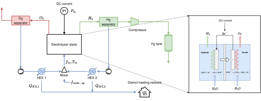
Figure 1: On the left: process sketch of the electrolyzer plant. On the right: working principle of an alkaline electrolytic cell. The reduction reaction happens at the cathode, where hydrogen is produced. The oxidation reaction happens at the anode, where oxygen is produced.

II Overview of water electrolysis

II-A Water electrolysis

The water splitting reaction is

$$\mathrm{H_{2}O(l)+\text{Electrical power}\longrightarrow H_{2}(g)+\frac{1}{2}O_{2}(g)}.$$ (1)

There are different technologies available to perform the reaction. We consider alkaline electrolysis. It is characterized by having two electrodes (cathode and anode), operating in a liquid alkaline electrolyte solution of potassium hydroxide (KOH), usually 20-40%, or sodium hydroxide (NaOH), separated by a diaphragm. It operates at relatively low temperatures (max $90{}^{\circ}C$). The working principle is depicted in Fig. 1. The half reactions are

Cathode (red.): $$\mathrm{2H_{2}O(l)+2e^{-}\longrightarrow H_{2}(g)+2OH^{-}(aq),}$$ (2)

Anode (ox.): $$\mathrm{2OH^{-}(aq)\longrightarrow 1/2O_{2}(g)+H_{2}O(l)+2e^{-}.}$$ (3)

II-B Process description

We consider the electrolyzer plant sketched in Fig. 1. The core of the process is the electrolyzer stack. It receives a flow of water and electric power. The produced hydrogen and oxygen gas leave the stack with the water stream, from their respective chambers. The two flows reach a respective gas/liquid separator, where the gas phase is separated from the liquid phase due to the different densities. The water outflows of the separators are recirculated back into the electrolyzer. The recirculated flows pass through heat exchangers, to remove excess heat produced in the electrolyzer, before they are mixed with fresh make-up water. The combined stream then enters the electrolyzer. The heat removed in the two heat exchangers is, ideally, recycled by sending it to the district heating network. The hydrogen gas leaving the hydrogen separator is compressed in a multistage compressor, to be stored under pressure in a hydrogen tank. From the storage tank the hydrogen can be distributed to downstream processes or other facilities, for example.

III Dynamic modeling

We investigate models for water electrolysis in the form of differential algebraic equations (DAE)

$$\dot{x} =f(x,y,u,d,p),$$ (4a)

$$0 =g(x,y,u,d,p).$$ (4b)

$x$ is the vector of differential variables, $y$ are algebraic variables, $u$ are manipulated variables (MVs), $d$ are the disturbances and $p$ is the vector of model parameters.

Additionally, the outputs of interest of the system may be denoted with

$$z=h(x,y,u,d,p).$$ (5)

III-A Modeling principles

Our modeling approach is based on physical first principles. We use mass and energy balances to model each component of the system. We review them here briefly, in order to present our formulation and notation.

We express the change in time of the number of moles in a physical system as

$$\dot{n}=f_{in}-f_{out}+R,$$ (6)

where $f_{in}$ and $f_{out}$ are the molar inlet and outlet mass flow rates and $R$ is the production rate. Notice that we always assume vector notation for handling different chemical species. The production rate is given by the stoichiometry and kinetics of the chemical reaction happening in the system, i.e.

$$R=S^{\prime}r,\qquad r=r(T,P,n).$$ (7)

$S$ is the stoichiometric matrix and $r$ is the reaction rate.

The total energy in a system is the sum of the potential, kinetic and internal energy

$$E=E_{p}+E_{k}+E_{e}+U.$$ (8)

We consider systems for which $E\approx U$ holds. The energy balance for such a system is

$$\dot{U}=\tilde{H}_{in}-\tilde{H}_{out}+Q+W_{s}+W_{e}.$$ (9)

We indicate with $\tilde{H}$ any enthalpy flow. $Q$ is any heat transferred to/from the external ambient, $W_{s}$ is the shaft work and $W_{e}$ is the electrical work.

III-B Thermodynamic functions

We rely on a thermodynamic library to evaluate all the thermodynamic functions. We use ThermoLib [10], a library implemented in Matlab and C that uses cubic equations of state to compute vapor and liquid phase thermodynamic properties. The library can also evaluate first and second order derivatives of the thermodynamic functions, which is often required when constructing the Jacobian of such dynamic models. ThermoLib evaluates the enthalpy, the entrophy and the volume as a function of the temperature $T$, pressure $P$ and number of moles $n$, i.e.,

$$H =H(T,P,n),$$ (10a)

$$S =S(T,P,n),$$ (10b)

$$V =V(T,P,n).$$ (10c)

Other thermodynamic properties can be easily derived.

$$U =H-PV,$$ (11a)

$$G =H-TS.$$ (11b)

$U$ is the internal energy, and $G$ is Gibbs’ free energy. Enthalpy flow rates are computed as

$$\tilde{H}=H(T,P,f).$$ (12)

IV Process modeling

This section deals with modeling the main components of an electrolyzer plant, as depicted in Fig. 1. We provide a description of each part and sum up the full model as a system of DAEs.

IV-A Electrolyzer stack

The electrolyzer stack consists of multiple electrolytic cells connected in series. The general working principle of an electrolytic cell is shown is Fig. 1, to the right.

The model consists of an electrochemical part, and mass and energy balance.

IV-A1 Electrochemical reaction

The minimum voltage requirement for reaction, called the reversible voltage, is computed by

$$\xi_{rev}=\frac{\Delta G_{r}}{zF}.$$ (13)

$\Delta G_{r}$ is the Gibbs’ free energy at the reaction conditions. $F$ is the Faraday constant and $z=2$ is the number of electrons transferred. $\Delta G_{r}$ is calculated based on the pure component enthalpies $H_{i}$ and entropies $S_{i}$ at given temperature $T$, operating pressure $P$ for liquid species and partial pressure $p_{i}$ for the gas species.

$$\Delta H_{r} =H_{H_{2}}(T,p_{H_{2}})(g)+\frac{1}{2}H_{O_{2}}(T,p_{O_{2}})(g)-H_{H_{2}O}(T,P)(l),$$ (14a)

$$\Delta S_{r} =S_{H_{2}}(T,p_{H_{2}})(g)+\frac{1}{2}S_{O_{2}}(T,p_{O_{2}})(g)-S_{H_{2}O}(T,P)(l),$$ (14b)

$$\Delta G_{r} =\Delta H_{r}-T\Delta S_{r}.$$ (14c)

(l) or (g) indicate liquid or gas species. The pressure and temperature dependence of the reversible voltage is considered by evaluating $H_{i}$ and $S_{i}$ at appropriate temperature and pressure. We assume that the gas phase in the cathode and the anode chamber is pure hydrogen and pure oxygen, respectively, therefore $p_{H2}=p_{O2}=P$. The enthalpy and entropy of water is calculated at operating pressure $P$, assuming that the presence of KOH in the solution can be neglected and water therefore behaves like an ideal liquid. We assume that the pressure is constant. ThermoLib is used to evaluate the $H_{i}$ and $S_{i}$, which has the added benefit that nonlinearities of the heat capacities, as modelled in the DIPPR database, are taken into account.

The total energy requirement is expressed by the reaction enthalphy

$$\Delta H_{r}=\Delta G_{r}+T\Delta S_{r}.$$ (15)

$T$ is the temperature and $\Delta S_{r}$ is the reaction entropy. The second term accounts for the irreversibilities of the reaction. This extra energy requirement is therefore brought as heat. The total voltage that one needs to provide if all the energy is transferred as electricity is called thermoneutral voltage

$$\xi_{tn}=\frac{\Delta H_{r}}{zF}.$$ (16)

The real total voltage of a single electrolytic cell takes into account extra irreversibilities [5]

$$\xi_{cell}(I,T)=\xi_{cell}=\xi_{rev}+\xi_{ohm}+\xi_{act}+\xi_{con}.$$ (17)

$\xi_{ohm}$ is the ohmic overvoltage. This is due to ohmic losses in the cell, generated by the resistance to the electron flux in the electrodes, the connectors and also by the resistance in the electrolyte and the diaphragm between the 2 chambers. $\xi_{act}$ is the activation overvoltage. It comes from the kinetics of the electric charge transfer that occurs at the electrode reaction sites. This in other words describes the activation barrier in the electrochemical reaction. $\xi_{con}$ is the concentration overvoltage. This is caused by mass transfer losses, and it happens only at very high current densities, hence it can be neglected for alkaline electrolyzers.

The following empirical model for the activation and ohmic overvoltages has been proposed by [5]

$$\xi_{ohm} =(r_{1}+r_{2}T)\frac{I}{A},$$ (18a)

$$\xi_{act} =s\log\left(\left(t_{1}+\frac{t_{2}}{T}+\frac{t_{3}}{T^{2}}\right)\frac{I}{A}+1\right).$$ (18b)

$A$ is the electrode area of a single cell, $I$ is the current. The parameters $r_{1}$ and $r_{2}$ represent the ohmic resistance, while $s$ and $t_{1},t_{2},t_{3}$ are the activation overvoltage coefficients. These are estimated empirically and depend on the specific electrolyzer. The voltage and the current are related to the input electric power

$$P_{in}=n_{c}\xi_{cell}(I,T)I.$$ (19)

$n_{c}$ is the number of (identical) electrolytic cells connected in series. The reaction rate is a function of the current

$$r(I)=n_{c}\frac{\eta_{F}}{zF}I.$$ (20)

The term $\eta_{F}$ is known as Faraday efficiency. This is

$$\eta_{F}=\frac{(I/A)^{2}}{f_{1}+(I/A)^{2}}f_{2}.$$ (21)

$f_{1}$ and $f_{2}$ are parameters.

The electrochemical dynamics enter the model as algebraic equations

$$g_{el}=\begin{bmatrix}\xi_{cell}(I,T)-\xi_{rev}(T)-\xi_{ohm}(I,T)-\xi_{act}(I,T)\\ P_{in}-n_{c}\xi_{cell}(I,T)I\end{bmatrix}=0.$$ (22)

IV-A2 Mass balance

We compute the outgoing flow streams from the anodic and cathodic chambers assuming steady state in the mass balance. We use vector notation with chemical species in the order [H₂O, H₂, O₂]^T, i.e.

$$n=\begin{bmatrix}n_{H_{2}O}\\ n_{H_{2}}\\ n_{O_{2}}\end{bmatrix}.$$ (23)

In the anodic chamber we have

$$\dot{n}^{an}=\frac{1}{2}f_{in}-f_{out}^{an}+R^{an}=0.$$ (24)

The outgoing flow is

$$f_{out}^{an}=\begin{bmatrix}f_{in,H_{2}O}/2\\ 0\\ 0\end{bmatrix}+\begin{bmatrix}1\\ 0\\ 1/2\end{bmatrix}r.$$ (25)

In the chatodic chamber we have

$$\dot{n}^{cat}=\frac{1}{2}f_{in}-f_{out}^{cat}+R^{cat}=0.$$ (26)

The outgoing flow is

$$f_{out}^{cat}=\begin{bmatrix}f_{in,H_{2}O}/2\\ 0\\ 0\end{bmatrix}+\begin{bmatrix}-2\\ 1\\ 0\end{bmatrix}r.$$ (27)

Notice that it is assumed that the inlet flow of water is split exactly in equal parts between the anode and cathode chambers. The total outgoing flow from the stack is

$$f_{out}=f_{out}^{an}+f_{out}^{cat}.$$ (28)

IV-A3 Energy balance

The energy balance in the electrolyzer is

$$\dot{U}_{el}=\tilde{H}_{in}-\tilde{H}_{out}+Q+W_{e}.$$ (29)

$U_{el}$ is the internal energy of the electrolyzer, $\tilde{H}_{in}$ and $\tilde{H}_{out}$ are the enthalpy flows in and out, $Q$ is heat flow exchanged with the ambient (convective) and $W_{e}$ is the electrical work. Specifically

$$W_{e}= P_{in},$$ (30a)

$$Q= -Q_{amb}=-A_{s}h_{c}(T-T_{amb}),$$ (30b)

$$\tilde{H}_{in}= H(T_{in},P,f_{in})=H(T_{in},P,f_{in,H_{2}O})(l),$$ (30c)

$$\tilde{H}_{out}= H(T,P,f_{out})=H(T,P,f_{out,H_{2}O})(l),$$ (30d)

$$+H(T,P,f_{out,H_{2}})(g)+H(T,P,f_{out,O_{2}})(g).$$

$A_{c}$ is the active area of heat transfer, $h_{c}$ is the heat transfer coefficient and $T_{amb}$ is the ambient temperature. The internal energy of the electrolyzer is a function of the form

$$U_{el}=U_{el}^{0}+C_{p,el}(T-T^{0}),$$ (31)

with

$$C_{P,el}=C_{P,H_{2}O}+C_{P,H_{2}}+C_{P,O_{2}}+C_{P,metal}.$$ (32)

We assume that the mass of fluids and the metal are constant, therefore $C_{P,el}$ can be considered constant. As a consequence, $\dot{U}_{el}=C_{P,el}\dot{T}$.

IV-B Liquid/gas separator

We model the liquid and gas hold-up in the oxygen and hydrogen separator tanks using mass and energy balance. The separators are modelled as ideal separators, hence the liquid/gas separation is perfect and all outflows are pure. In order to not use any compressor, the separator tanks have to hold a pressure that is never higher than the pressure in the electrolyzer $P$. We hereby report the equations for the hydrogen separator (Fig. 2).

$$\dot{n}_{sep,2} =f^{cat}_{out}-f_{sep,2},$$ (33a)

$$\dot{U}_{sep,2} =\tilde{H}_{in}-\tilde{H}_{out}$$

$$=H(T,P,f^{cat}_{out})-H(T_{sep,2},P,f_{sep,2}).$$ (33b)

The tank is assumed to be adiabatic. Notice that the first equation is vectorial and that the outlet flow is

$$f_{sep,2}=\begin{bmatrix}f^{sep,2}_{H_{2}O}\\ f^{sep,2}_{H_{2}}\\ 0\end{bmatrix}.$$ (34)

The liquid outflow $f^{sep,2}_{H_{2}O}$ is a manipulated variable, while the gas outflow $f^{sep,2}_{H_{2}}$ comes as a consequence of fixing the pressure. The algebraic equations for the separator are

$$g_{sep,1}=\begin{bmatrix}U_{TL}-U_{sep,2}\\ V_{TL}-V_{tot,2}\end{bmatrix}=0.$$ (35)

The energy and volume evaluated by the thermodynamic library are

$$U_{TL}= U(T_{sep,2},P,n^{sep,2,}_{H_{2}O})(l)+U(T_{sep,2},P,n^{sep,2}_{H_{2}})(g),$$ (36a)

$$V_{TL}= V(T_{sep,2},P,n^{sep,2}_{H_{2}O})(l)+V(T_{sep,2},P,n^{sep,2}_{H_{2}})(g).$$ (36b)

The model for the gas-liquid separator for the oxygen stream is exactly the same, and we distinguish its variables by using the index 1.

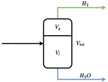
Figure 2: Gas-liquid separator for the hydrogen stream out of the electrolyzer.

IV-C Compressor

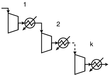
Figure 3: Multi-stage compressor with heat exchangers.

The hydrogen that flows out of the separator needs to be compressed, before reaching the storage tank. Since the pressure requirement in such a tank can be very high, a multi-stage compressor is required. Figure 3 shows a $k$-stage compressor with cooling elements. Notice that determining the right amount of compressors to be used is a sizing problem. We choose 3 identical compressors. We model each compressor as isentropic (ideal and static), that means that the entropy stays constant during the compression process. For each stage $k$, we get an algebraic equation

$$g_{k,comp}=\tilde{S}_{k,out}-\tilde{S}_{k,in}=0.$$ (37)

The entrophy flows are such that

$$\tilde{S}_{k,in} =S(T_{k,in},P_{k,in},f_{H_{2}}^{sep,2}),$$ (38a)

$$\tilde{S}_{k,out} =S(T_{k,comp},P_{k,out},f_{H_{2}}^{sep,2}).$$ (38b)

$T_{k,in},P_{k,in}$ and $T_{k,comp},P_{k,out}$ are the temperature and pressure at the inlet and the outlet, respectively, of each compressor stage $k$. The enthalphy change

$$\tilde{H}_{k,out}=\tilde{H}_{k,in}+\eta W_{comp,k}$$ (39)

allows us to compute the work $W_{comp,k}$ that every compressor has to perform. $\eta$ is the efficiency of the compressor. The enthalpy flows are such that

$$\tilde{H}_{k,in} =H(T_{k,in},P_{k,in},f_{H_{2}}^{sep,2}),$$ (40a)

$$\tilde{H}_{k,out} =H(T_{k,out},P_{k,out},f_{H_{2}}^{sep,2}).$$ (40b)

The intermediate cooling work by the heat exchangers between the stages can be computed, for each stage, as

$$W_{hex,k}=\Delta H_{hex,k}=\tilde{H}_{k+1,in}-\tilde{H}_{k,out}.$$ (41)

The last heat exchanger cools down to the tank temperature, therefore

$$\tilde{H}_{4,in}=H(T_{tank},P_{tank},f_{H_{2}}^{sep,2}).$$ (42)

IV-D Storage tank

The mass and energy balance in the tank give the following differential equations

$$\dot{n}_{tank}= f^{sep,2}_{H_{2}}-f_{H_{2}}^{tank},$$ (43a)

$$\dot{U}_{tank}= \tilde{H}_{in}-\tilde{H}_{out}-Q_{amb}=H(T_{tank},P_{tank},f^{sep,2}_{H_{2}})-$$ (43b)

$$H(T_{tank},P_{tank},f_{H_{2}}^{tank})-h_{tank}A_{tank}(T_{tank}-T_{amb}).$$

$h_{tank}$ is the heat transfer coefficient of the tank and $A_{tank}$ is the transfer area. The following extra algebraic equations are necessary to solve the system

$$g_{tank}=\begin{bmatrix}U_{TL}-U_{tank}\\ V_{TL}-V_{tank}\end{bmatrix}=0.$$ (44)

The energy and volume evaluated by the thermodynamic library are

$$U_{TL} =U(T_{tank},P_{tank},n_{tank}),$$ (45a)

$$V_{TL} =V(T_{tank},P_{tank},n_{tank}).$$ (45b)

IV-E Heat exchangers

The purpose of the heat exchangers is to remove excess heat, produced by the reaction, from the water that is being recirculated back to the electrolyzer, hence the water outflows of the two separators.

We model the 2 heat exchangers with a static energy balance. The temperatures of the flows after the heat exchangers $T_{HX,1}$ and $T_{HX,2}$ are such that

$$g_{HX}=\begin{bmatrix}\begin{matrix}\tilde{H}_{HX,1}-H(T_{sep,1},P,f^{sep,1}_{H_{2}O})-Q_{HX,1}\end{matrix}\\ \begin{matrix}\tilde{H}_{HX,2}-H(T_{sep,2},P,f^{sep,2}_{H_{2}O})-Q_{HX,2}\end{matrix}\end{bmatrix}=0.$$ (46)

$Q_{HX,1}$ and $Q_{HX,2}$ are the heat flows to be removed and are considered as manipulated variables. The outlet enthalphy flows are

$$\tilde{H}_{HX,1}= H(T_{HX,1},P,f^{sep,1}_{H_{2}O})$$ (47a)

$$\tilde{H}_{HX,2}= H(T_{HX,2},P,f^{sep,2}_{H_{2}O})$$ (47b)

IV-F Flow mixer

The mixing point before the electrolyzer stack inlet is modelled using static mass and energy balance. The following algebraic equations arise

$$g_{mixer}=\begin{bmatrix}f_{in,H_{2}O}-f_{make-up}-f^{sep,1}_{H_{2}O}-f^{sep,2}_{H_{2}O}\\ \begin{matrix}\hfill H(T_{in},P,f_{in,H_{2}O})-\tilde{H}_{HX,1}-\tilde{H}_{HX,2}\\ \hfill-H(T_{make-up},P,f_{make-up})\end{matrix}\end{bmatrix}=0.$$ (48)

IV-G Full DAE system

The full DAE system consists of 24 equations. The differential variables are

$$\begin{split}x=[T,n^{sep,1}_{H_{2}O},n^{sep,1}_{O_{2}},U_{sep,1},n^{sep,2}_{H_{2}0},n^{sep,2}_{H_{2}},\\ U_{sep,2},n_{tank},U_{tank}]^{T}.\end{split}$$ (49)

The algebraic variables are

$$\begin{split}y=[&\xi_{cell},I,T_{sep,1},f^{sep,1}_{O_{2}},T_{sep,2},f^{sep,2}_{H_{2}},T_{1,comp},T_{2,comp},\\ &T_{3,comp},T_{tank},P_{tank},T_{HX,1},T_{HX,2},f_{in,H_{2}O},T_{in}]^{T}.\end{split}$$ (50)

The manipulated variables (inputs) are

$$u=[f^{sep,1}_{H_{2}O},f^{sep,2}_{H_{2}O},f_{make-up},f_{H_{2}}^{tank},Q_{HX,1},Q_{HX,2}]^{T}.$$ (51)

The disturbances are

$$d=[T_{amb},P_{in},T_{make-up}]^{T}.$$ (52)

The output of interest of the system is

$$z=f_{out,H_{2}}.$$ (53)

V Simulation results

We use the model parameters from [7] for the electrolyzer stack. Fig. 4 shows steady state plots between the main variables of the electrolyzer stack, for different values of the operating temperature. Notice how higher efficiency is observed at lower operating power.

We run a dynamic simulation of the model with step power input from 0.5 to 2.5 MW at $P=1$ atm. We plot in Fig. 5 the variables related to the electrolyzer stack, that is the operating temperature $T$, the cell voltage $\xi_{cell}$ and the current $I$. We set the manipulated variables such that $f_{in,H_{2}O}=$1.5 kg/s and $T_{in}=$ 40^∘C. The sudden change in power is reflected immediately in the hydrogen production rate, as the reaction rate directly depends on the current.

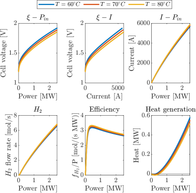
Figure 4: Steady state diagrams of the electrolyzer stack, for different values of the operating temperature $T$.

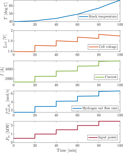
Figure 5: Electrolyzer dynamic simulation using step power input.

VI Conclusion

In this paper, we present a dynamic model for an alkaline electrolyzer plant. Each part of the plant is modeled using mass and energy balance. Thermodynamic properties (enthalpy, volume and internal energy) of the liquid and gases are evaluated using the thermodynamic library ThermoLib. We formulate the model as system of DAEs. We show steady state diagrams for the electrolyzer stack and perform a dynamic simulation with variable input power.

The plant-wide dynamic model can be used to perform process simulation and optimization. Future work includes developing a non-linear model predictive control algorithm tailored to this DAE model.

References

- [1] P. Olivier, C. Bourasseau, and P. B. Bouamama, “Low-temperature electrolysis system modelling: A review,” Renewable and Sustainable Energy Reviews, vol. 78, pp. 280–300, 2017.
- [2] M. David, C. Ocampo-Martínez, and R. Sánchez-Peña, “Advances in alkaline water electrolyzers: A review,” Journal of Energy Storage, vol. 23, pp. 392–403, 2019.
- [3] A. E. Samani, A. D’Amicis, J. D. De Kooning, D. Bozalakov, P. Silva, and L. Vandevelde, “Grid balancing with a large-scale electrolyser providing primary reserve,” IET Renewable Power Generation, vol. 14, no. 16, pp. 3070–3078, 2020.
- [4] A. Gloppen Johnsen, L. Mitridati, D. Zarrilli, and J. Kazempour, “The Value of Ancillary Services for Electrolyzers,” arXiv e-prints, p. arXiv:2310.04321, Oct. 2023.
- [5] Øystein Ulleberg, “Modeling of advanced alkaline electrolyzers: a system simulation approach,” International Journal of Hydrogen Energy, vol. 28, no. 1, pp. 21–33, 2003.
- [6] G. Sakas, A. Ibáñez-Rioja, V. Ruuskanen, A. Kosonen, J. Ahola, and O. Bergmann, “Dynamic energy and mass balance model for an industrial alkaline water electrolyzer plant process,” International Journal of Hydrogen Energy, vol. 47, no. 7, pp. 4328–4345, 2022.
- [7] M. Rizwan, V. Alstad, and J. Jäschke, “Design considerations for industrial water electrolyzer plants,” International Journal of Hydrogen Energy, vol. 46, no. 75, pp. 37120–37136, 2021. International Symposium on Sustainable Hydrogen 2019.
- [8] C. Huang, X. Jin, Y. Zong, S. You, C. Træholt, and Y. Zheng, “Operational flexibility analysis of alkaline electrolyzers integrated with a temperature-stabilizing control,” Energy Reports, vol. 9, pp. 16–20, 2023.
- [9] R. Qi, J. Li, J. Lin, Y. Song, J. Wang, Q. Cui, Y. Qiu, M. Tang, and J. Wang, “Thermal modeling and controller design of an alkaline electrolysis system under dynamic operating conditions,” Applied Energy, vol. 332, p. 120551, 2023.
- [10] T. K. Ritschel, J. Gaspar, and J. B. Jørgensen, “A thermodynamic library for simulation and optimization of dynamic processes.,” IFAC-PapersOnLine, vol. 50, no. 1, pp. 3542–3547, 2017. 20th IFAC World Congress.