MEGA: A Memory-Efficient GNN Accelerator Exploiting Degree-Aware Mixed-Precision Quantization

Abstract

Graph Neural Networks (GNNs) are becoming a promising technique in various domains due to their excellent capabilities in modeling non-Euclidean data. Although a spectrum of accelerators has been proposed to accelerate the inference of GNNs, our analysis demonstrates that the latency and energy consumption induced by DRAM access still significantly impedes the improvement of performance and energy efficiency. To address this issue, we propose a Memory-Efficient GNN Accelerator (MEGA) through algorithm and hardware co-design in this work. Specifically, at the algorithm level, through an in-depth analysis of the node property, we observe that the data-independent quantization in previous works is not optimal in terms of accuracy and memory efficiency. This motivates us to propose the Degree-Aware mixed-precision quantization method, in which a proper bitwidth is learned and allocated to a node according to its in-degree to compress GNNs as much as possible while maintaining accuracy. At the hardware level, we employ a heterogeneous architecture design in which the aggregation and combination phases are implemented separately with different dataflows. In order to boost the performance and energy efficiency, we also present an Adaptive-Package format to alleviate the storage overhead caused by the fine-grained bitwidth and diverse sparsity, and a Condense-Edge scheduling method to enhance the data locality and further alleviate the access irregularity induced by the extremely sparse adjacency matrix in the graph. We implement our MEGA accelerator in a 28nm technology node. Extensive experiments demonstrate that MEGA can achieve an average speedup of $38.3\times$, $7.1\times$, $4.0\times$, $3.6\times$ and $47.6\times$, $7.2\times$, $5.4\times$, $4.5\times$ energy savings over four state-of-the-art GNN accelerators, HyGCN, GCNAX, GROW, and SGCN, respectively, while retaining task accuracy.

I Introduction

Recently, Graph Neural Networks (GNNs) have attracted much attention from both industry and academia due to their superior learning and representing ability for non-Euclidean geometric data. A number of GNNs have been widely used in practical application scenarios, such as social network analysis[35, 14], autonomous driving[53], and recommendation systems[25, 59]. Many of these tasks demand low-latency and energy-efficient inference, especially for edge computing like autonomous driving [33, 53].

As presented in MPNN framework[17], the inference process of GNNs contains two phases: aggregation and combination, which exhibits unique computational characteristics compared to other DNNs such as CNN [34, 46, 22] and Transformer [49, 12, 29]. In the aggregation phase, each node in the graph collects information from its neighboring nodes according to the connections. Then, in the combination phase, the collected features of a node are updated using a combination function such as MLP. For the real-world graph, the connections are extremely sparse and unstructured. While the high sparsity can be leveraged for reducing computations in the aggregation phase, the complex data structure poses a significant challenge to memory access, leading to unexpected latency and energy cost, especially for general processors like CPU/GPU [40, 57]. In addition, a real-world graph often contains a vast volume of nodes, e.g., the Reddit dataset has 232965 602-dimensional nodes, which exacerbates the complexity of memory access in the combination phase. Therefore, addressing the memory bottlenecks in both phases is critical for fast and energy-efficient GNN inference.

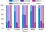
(a) Execution Cycle

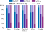
(b) Energy Consumption

Figure 1: The cycle and energy breakdown of HyGCN and GCNAX on different tasks.

Recently, a spectrum of dedicated GNN accelerators has been proposed to improve performance and energy-efficiency [56, 36, 61, 23, 16, 37, 60, 62, 7, 6, 38, 42]. HyGCN [56] is one of the first domain-specific accelerators for GNNs, which designs separate engines for aggregation and combination, respectively, to pipeline the two phases of the forward pass. GCNAX [36] models the execution cycle and DRAM access according to the loop optimization and then explore the design space by enumeration to find an optimal execution method. Although these works have optimized the GNN inference at the software and hardware levels, our analysis reveals that the performance and energy bottleneck caused by DRAM access is still very serious. As shown in Fig. 1, the stall caused by DRAM access accounts for up to 86.2% of the overall execution cycles on HyGCN. Worse still, the energy consumption of DRAM access also dominates the overall energy consumption, e.g., 90.2% for HyGCN on Reddit.

As a promising technique to achieve memory-efficient inference, network quantization that converts floating-point values into low-precision fixed-point counterparts can effectively reduce memory footprint and bandwidth requirement. Unfortunately, current methods for GNN quantization, such as DQ[47] and LP[65], are only capable of quantizing the model to 8bit without accuracy loss. If the compression ratio is further increased, such as quantized to 4bit, the model accuracy will significantly decline. Through an in-depth analysis of the graph nodes, we note that the uniform quantization (a specific quantization bitwidth is shared among all nodes) in existing works fails to distinguish the importance of the nodes. In this scenario, the nodes that are more sensitive to quantization will impede the overall bitwidth reduction. Besides, allocating the same bitwidth to the less important nodes will lead to considerable memory costs. Therefore, taking advantage of the node characteristics for quantization is essential to achieve a higher compression ratio while maintaining accuracy.

To unleash the potential of GNN acceleration, in this paper, we propose a Memory-Efficient GNN Accelerator (MEGA) through algorithm and hardware co-design. At the algorithm level, we develop a Degree-Aware mixed-precision quantization method for GNN compression. Our key observation is that nodes with higher in-degrees, which we refer to as important nodes, tend to have larger average values of features after aggregation, and a smaller fraction of nodes in a graph are deemed important. This motivates a mixed-precision quantization method, in which a proper bitwidth is learned and allocated to a node according to its in-degree to compress the network as much as possible while retaining accuracy. At the hardware level, we employ a heterogeneous architecture design in which the aggregation and combination phases are implemented separately with different dataflows. In particular, bit-serial computation is exploited in the combination phase for precision-scalable inference. We also present an Adaptive-Package method to alleviate the storage overhead induced by the fine-grained bitwidth and diverse sparsity, and a Condense-Edge scheduling method to enhance the data locality and further reduce DRAM accesses.

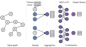
Figure 2: Illustration of the GNN models.

In summary, the contributions of this paper are as follows:

• We give an in-depth analysis of the limitations in previous GNNs quantization methods and then propose the Degree-Aware mixed-precision quantization method to enable adaptive learning of quantization parameters for nodes with different degrees, which can improve the model compression ratio as much as possible while maintaining the model accuracy.

• We propose an accelerator named MEGA co-designed with our Degree-Aware mixed-precision quantization method. It employs a heterogeneous architecture that computes the combination and aggregation phases separately using different dataflows. To mitigate the complexity caused by the mixed-precision node features under diverse sparsity, we propose an Adaptive-Package format to improve the efficiency of storage and memory access. Moreover, we design a Condense-Edge scheduling strategy in MEGA to further reduce the DRAM access.

• The experimental results demonstrate that our Degree-Aware quantization can achieve up to 15.8% improvement in accuracy along with a larger compression ratio (up to $18.6\times$ v.s. $8\times$) compared to the state-of-the-art quantization method [47]. We also implement MEGA on a 28nm technology node and evaluate on five real-world datasets and three GNN models. On average, our MEGA can achieve $38.3\times$, $7.1\times$, $4.0\times$, $3.6\times$ speedups and $47.6\times$, $7.2\times$, $5.4\times$, $4.5\times$ energy savings over HyGCN[56], GCNAX[36], GROW[23], and SGCN[60], respectively.

II Background and Related Work

II-A Graph Neural Networks

Most GNNs can be presented using the MPNN framework[17], in which the forward pass in each layer contains two phases as shown in Fig. 2. First, each node collects information from neighboring nodes and uses the aggregation function to generate hidden features in the aggregation phase. Second, in the combination phase, the hidden features are transformed into new features by the combination function. In order to reduce the computational complexity, sometimes the neighboring nodes are sampled before aggregating, then only the sampled neighbors are used in the aggregation phase. In this paper, we focus on the inference acceleration of three typical GNN models, i.e., Graph Convolution Network (GCN)[32], Graph Isomorphism Network (GIN)[55], and GraphSage[20].

The forward pass of the three models can be uniformly represented as follows:

$${\mathbf{X}^{(l)}}=\sigma(\tilde{\mathbf{A}}{\mathbf{X}^{(l-1)}}{\mathbf{W}^{(l-1)}})\text{,}$$ (1)

where $\tilde{\mathbf{A}}$ is the normalized adjacency matrix, $\mathbf{X}^{(l-1)}$ and $\mathbf{W}^{(l-1)}$ are the feature map including all nodes features and the learned parameters of the $(l-1)$-th layer, respectively, and the $\sigma$ is an activation function, e.g., ReLU.

For the computation of $\tilde{\mathbf{A}}\mathbf{X}\mathbf{W}$, there are two execution patterns, $(\tilde{\mathbf{A}}\mathbf{X})\mathbf{W}$ and $\tilde{\mathbf{A}}(\mathbf{X}\mathbf{W})$. We choose $\tilde{\mathbf{A}}(\mathbf{X}\mathbf{W})$ in our accelerator design, which greatly reduces the number of MACs for the GNNs of our focus that have two or three layers and the dimension of input features is much larger than the hidden features, as reported in [16, 23, 36].

II-B Quantization

Although some works have applied the quantization technique to GNNs, there remain some issues that hinder the release of the potential to accelerate the inference and reduce the memory requirement. SGQuant [15] only quantizes the nodes features and still employs floating-point computation during inference, which is limited in improving the energy efficiency[21]. DQ [47] proposes a degree-quant training strategy, which generates masks for nodes with high degrees and only quantizes the nodes without masks. This method can quantize GNNs to 8bit with negligible accuracy degradation. However, when quantizing GNNs to lower bitwidth, the accuracy of DQ drops severely. There are also some works[52, 3, 51, 26] that quantize GNNs to 1-bit. Though the compression ratio is high, these methods will cause unacceptable accuracy degradation on complex GNN models, e.g., GIN and GraphSage, which obstructs their generalization.

Moreover, based on the idea that different layers have different sensitivities to quantization, mixed-precision quantization is proposed in CNNs to quantize different layers with different bitwidths [48, 13, 24, 11, 10, 8, 9]. However, due to the vast differences between GNNs and CNNs, e.g., the extremely sparse connections among nodes, it is difficult to use these methods on GNNs directly.

II-C Hardware Acceleration of GNNs

There are many previous works [56, 36, 61, 23, 16, 37, 60, 62, 7, 6, 38, 42] that design dedicated hardware accelerators for GNNs. HyGCN[56] is one of the first domain accelerators that proposes the window sliding method to eliminate zeros. However, ignoring the sparsity existing in nodes features results in low utilization of its process engines and severe pipeline stalls. GCNAX[36] models the execution cycle and DRAM access according to the loop tile and explores the design space by enumeration to find the optimal tiling pattern. However, GCNAX cannot handle the irregular memory access caused by the extremely sparse adjacency matrix. GCoD[61] proposes a co-design framework, which can prune, cluster the adjacency matrix at the algorithm level by using the graph partition algorithm, and separately process the dense region and sparse region through dedicated hardware design. GROW[23], which adopts the row product to perform the two phases of GNNs, also employs the same graph partition algorithm to improve the locality of its dataflow. However, the more sparse connections among different subgraphs will lead to severe DRAM accesses and hinder the improvement of performance and energy efficiency. SGCN[60] employs a feature compression format to reduce off-chip traffic and designs a dedicated accelerator to process the compressed features efficiently. However, adopting a systolic array to perform the combination phase results in SGCN not being able to exploit the sparsity in the combination phase.

TABLE I: The accuracies and compression ratios of GIN when using DQ with different quantization bitwidths trained on CiteSeer (CR: Compression Ratio, Acc: Accuracy).

	FP32	8bit	7bit
Acc	66.1±0.9%	67.5±1.4%	65.0±2.4%
CR	1x	4x	4.6x
	6bit	5bit	4bit
Acc	63.8±3.3%	63.7±3.4%	60.8±2.1%
CR	5.3x	6.4x	8x

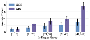
Figure 3: Average node feature values with respect to different in-degrees after aggregation. The average values are all generated from 100 runs.

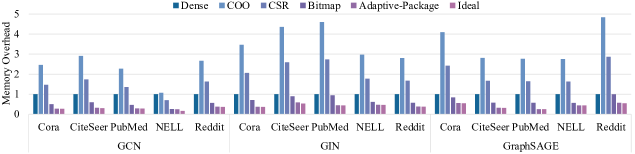
Figure 4: Comparisons of various sparse data representations on three models (normalized to Dense). Ideal: only quantized non-zero values are stored. Adaptive-Package is our proposed method.

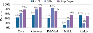
Figure 5: Comparison of sparsity across various datasets on different models.

III Motivation

III-A Rethinking GNN Quantization

Despite the promising benefits of network quantization in achieving memory-efficient inference, prior works have overlooked the potential of utilizing quantization for GNN accelerator design. Although there are some works on GNN quantization, we observe that these existing methods still have limitations. For example, the state-of-the-art method DQ[47] can compress the model from FP32 to 8bit with negligible accuracy loss. When the quantization bitwidth decreases, the accuracy degradation will rise up to 5.3% (4bit), as shown in TABLE I. Considering the vast amount of DRAM accesses involved in GNN inference, achieving a higher compression ratio while maintaining accuracy is crucial to improving performance and energy efficiency.

Note that in existing GNN quantization methods [47, 15], a specific quantization bitwidth is shared among all nodes in a graph without considering the graph topology. Through an in-depth analysis of the node property, we observe that the data-independent quantization is not optimal in terms of accuracy and energy efficiency. Fig. 3 visualizes the average aggregated value of node features with respect to different in-degrees for GCN [32] and GIN [55] on the Cora dataset. It can be noticed that as the in-degree of a node increases, the feature value gets larger after aggregation. This indicates that nodes with different in-degrees have different ranges of feature values, thus a uniform quantization bitwidth cannot fit the data distribution well. Moreover, according to [54, 2], the in-degrees of nodes in most real-world graphs often follow the power-law distribution, i.e., nodes with a low in-degree account for the majority of graph data. Obviously, a uniform quantization bitwidth (such as 8bit) for all nodes will cause a significant waste on storage and memory accesses.

Intuitively, to achieve a high compression ratio while retaining accuracy, we can adopt different bitwidths to quantize the nodes with varying degrees, since the feature values of a node are closely related to its degree. However, due to the vast volume of nodes in real-world graphs, manually assigning bitwidths to different nodes will result in model accuracy degradation and cannot compress the models to the maximum extent. Accordingly, we propose the Degree-Aware mixed-precision quantization method in which a proper quantization bitwidth and the associated scale are automatically learned and assigned to each node in a graph. To the best of our knowledge, we are the first to introduce mixed-precision quantization to GNN accelerator design.

III-B Challenges on Accelerator Design

Although there have been considerable CNN accelerators that support precision-scalable[27, 44, 43] or sparse computation[21, 64, 30, 63], these accelerators cannot be used directly for GNN acceleration due to the unique computation and sparse patterns inherent in GNNs, as previously reported[1, 18, 54]. Furthermore, none of the existing GNN accelerators support mixed-precision data format in both computation and storage, impeding the acceleration potentials of our Degree-Aware method. Therefore, a dedicated accelerator co-designed with our proposed algorithm is essential. However, challenges still remain:

1) Challenge on storage: Properly storing the fine-grained mixed-precision features is critical to achieving optimal efficiency in GNN accelerator design. However, two challenges on storage hinder the gains from highly compressed features. First, the existing sparse data representations cannot handle the fine-grained bitwidth so the highest quantization bitwidth among all nodes should be used when storing the quantized features, leading to non-negligible storage underutilization. As shown in Fig. 4, existing compression formats are far from ideal in the mixed-precision scenario. Second, identifying the location of non-zero values is challenging. As shown in Fig. 5, the sparsity of nodes features, i.e., $\mathbf{X}$, varies greatly across different tasks. Along with the fine-grained bitwidth, the various sparsity will lead to more irregular and random access to the memory and significant overhead on decoding the quantized features.

2) Challenge on irregular memory access: A great deal of irregular memory accesses to nodes features introduced by the extremely sparse connections result in a significant discount of the improvement in performance and energy savings. In previous works, such as GROW[23] and GCoD[61], the graph partition algorithm is used to divide the graph into several subgraphs, in which the data locality is significantly improved. However, this results in more sparse connections between subgraphs (referred to as sparse connections), as the total number of edges in the graph remains unchanged. The sparse connections weaken the spatial locality and significantly decrease the data reuse, causing more off-chip memory traffic. Taking GROW[23] as an example, we compare the number of DRAM accesses induced by the dense subgraphs and the sparse connections in the aggregation phase with and without using the graph partition algorithm METIS[28] in Fig. 6. We can notice that although the overall DRAM accesses can be reduced after graph partition, there are still considerable DRAM accesses caused by sparse connections.

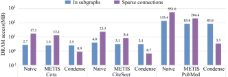
Figure 6: Comparisons of DRAM access on three configs. Naive: without graph partition. METIS: divide the graph by METIS. Condense: our Condense-Edge method.

In this paper, we present two techniques to address the above issues. Specifically, we propose a memory-efficient Adaptive-Package format that can efficiently encode/decode the mixed-precision sparse node features and achieve near-ideal storage utilization (as shown in Fig. 4). We also propose a Condense-Edge scheduling method capable of significantly reducing the overhead caused by sparse connections (as shown in Fig. 6). We will elaborate these techniques in Section V-B and V-E.

IV Degree-Aware Quantization

In this section, we present our Degree-Aware mixed-precision quantization approach, which quantizes nodes with different in-degrees by different learnable quantization parameters, including bitwidth and scale. These parameters can be learned during training. By imposing a penalty on memory size, our approach is memory-aware, which allows us to obtain a better trade-off between memory footprint and model accuracy.

Given a graph with $N$ nodes, we assume that the node features are $F$-dimensional, then the feature map is denoted as $\mathbf{X}\in\mathbb{R}^{N\times F}$, and ${\bm{x}}_{i}$ is the features of node $i$. Firstly, we initialize the learnable quantization parameters, i.e., scale ${\bm{s}}=(s_{1},s_{2},…,s_{d})$, and bitwidth $\mathbf{b}=(b_{1},b_{2},…,b_{d})$, where $d$ is the maximum degree of nodes in a graph. We quantize nodes with different degrees as follows:

$$\bar{{\bm{x}}}_{i}=sign({\bm{x}}_{i})\begin{cases}\lfloor\frac{\left|{\bm{x}}_{i}\right|}{\alpha_{i}}+0.5\rfloor\text{,}\left|{\bm{x}}\right|<\alpha_{i}(2^{[b_{i}]-1}-1)\\ \\ 2^{[b_{i}]-1}-1\text{,}\left|{\bm{x}}_{i}\right|\geq\alpha_{i}(2^{[b_{i}]-1}-1)\end{cases}\ \text{,}$$ (2)

where $(\alpha_{i},b_{i})$ are the quantization parameters selected based on the degree of the node, i.e., $\alpha_{i}=s_{d_{i}}$ and $b_{i}=b_{d_{i}}$, $d_{i}$ is the degree of the $i$-th node. Then we can obtain the fixed-point feature map $\bar{\mathbf{X}}$, and the original feature can be represented as ${\bm{X}}_{q}={\bm{S}}_{X}\cdot\bar{\mathbf{X}}$, where ${\bm{S}}_{X}=diag(\alpha_{1},\alpha_{2},...,\alpha_{N})$. Fig. LABEL:quantize displays the Degree-Aware quantization process.

In the combination phase, the core calculation is $\mathbf{X}\mathbf{W}$, where $\mathbf{X}$ is the feature map obtained from the aggregation phase of the previous layer. In order to further decrease the redundant DRAM accesses, we also quantize $\mathbf{W}$. Given that $\mathbf{W}$ in a specific layer is shared among all nodes, we quantize $\mathbf{W}$ to the same bitwidth of 4bits for all GNNs in this paper. Moreover, to enhance the generalization, each column of $\mathbf{W}$ is endowed with its individual learnable quantization scale, i.e., ${\bm{s}}_{W}=(\beta_{1},\beta_{2},..,\beta_{F_{2}})$, where $F_{2}$ is the output-dimension of the node features in the current layer and $\beta_{i}$ is the quantization scale for the $i$-th column of $\mathbf{W}$. We can obtain the integer representation $\bar{\mathbf{W}}$ as Eq 2 and the quantized representation ${\bm{W}}_{q}=\bar{\mathbf{W}}\cdot{\bm{S}}_{W}$, where ${\bm{S}}_{W}=diag(\beta_{1},\beta_{2},...,\beta_{F_{2}})$. The float-point matrix multiplication in the combination phase can be reformulated as follow:

$$\mathbf{X}\cdot\mathbf{W}\approx{\bm{X}}_{q}\cdot{\bm{W}}_{q} =({\bm{S}}_{X}\cdot\bar{\mathbf{X}})\cdot(\bar{\mathbf{W}}\cdot{\bm{S}}_{W})$$ (3)

$$=(\bar{\mathbf{X}}\cdot\bar{\mathbf{W}})\odot({\bm{s}}_{X}\otimes{\bm{s}}_{W})\ \text{,}$$

where $\odot$ denotes an element-wise multiplication, and $\otimes$ denotes the outer product. An execution example is illustrated in Fig. LABEL:matrix_mult. For the aggregation phase, i.e., $\mathbf{A}\mathbf{B}$, where $\mathbf{B}=\mathbf{XW}$ and $\mathbf{A}\in\{0,1\}^{N\times N}$ is the adjacency matrix, we quantize $\mathbf{B}$ as the quantization way of $\mathbf{W}$. Then the aggregation phase can also be performed by integer operations to reduce the computational overhead.

After quantization, the inference process of GNNs can be executed using fixed-point operations, resulting in a significant reduction in energy consumption for arithmetic operations, and a noteworthy decrease in DRAM access.

To better trade off the model accuracy and the memory reduction, our Degree-Aware method introduces a penalty on memory size to the loss function:

$${{L}_{memory}}={{(\frac{1}{\eta}\cdot\sum\limits_{l=1}^{L}{\sum\limits_{i=1}^{N}{\dim^{l}\cdot b_{i}^{l}}}-{{M}_{target}})^{2}}}\ \text{,}$$ (4)

where $L$ is the number of layers in the GNNs, $N$ is the total number of nodes, $\dim^{l}$ is the length of the node features in $l$-th layer, $b_{i}^{l}$ is the quantization bitwidth for node $i$ in $l$-th layer, $M_{target}$ is the target memory size on the total node features memory size, and $\eta=8*1024$, which is a constant to convert the unit of memory size to $\rm KB$. Then the model and quantization parameters can be trained by the loss function:

$$L_{total}={{L}_{task}}+\lambda\cdot{L}_{memory}\ \text{,}$$ (5)

where $L_{task}$ is the task-related loss function and $\lambda$ is a penalty factor on $L_{memory}$.

V MEGA Architecture

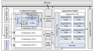
Figure 8: Overall Architecture of MEGA Accelerator.

(a) Nodes features

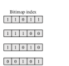
(b) Bitindex

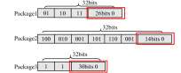
(c) Fixed length package

(d) Adaptive length package

Figure 9: (a) The fine-grained mixed-precision quantization nodes features. (b) Bitmap index. (c) The paddings in the package with fixed length. (d) The Adaptive-Package method in this work.

V-A Overview

As illustrated in Fig. 8, the accelerator employs a heterogeneous architecture, in which the combination and aggregation phases are performed in the Combination Engine and the Aggregation Engine, respectively. Similar to the previous works[16, 23, 36], MEGA adopts the execution order of $\mathbf{A}(\mathbf{X}\mathbf{W})$ to reduce the number of MACs for better efficiency. The workflow of MEGA is as follows.

The encoded input nodes and network weights prefetched from the off-chip DRAM are stored in the Input and Weight Buffer, respectively. When the calculation starts, the node features are read from the Input Buffer and dispatched to the parallel Combination Tiles in the Combination Engine, each tile is responsible for processing a slice of features in a node. After decoding, the node features in a tile are fed to the Combination Unit and perform the combination operation, i.e., $\mathbf{B=XW}$, with the corresponding weights. To exploit the potential benefits introduced by the high sparsity of nodes features, the Combination Engine employs the row product dataflow, which is more suitable for the wide range of sparsity variation in features, as reported in [23, 60, 37]. The results from different Combination Tiles can be added together to generate the final results or partial sums of one node once slices in different tiles all have been processed done, which enhances the temporal locality.

During aggregation, we divide the graph into several subgraphs and perform aggregation one subgraph after another. Once a node finishes the combination phase, the combined node features are sent to the Aggregation Engine to perform aggregation. These features are simultaneously stored in the Combination Buffer or reordered in the Sparse Buffer by the Condense Unit through our proposed Condense-Edge scheduling strategy, which enhances data locality and makes memory access contiguous when aggregating other subgraphs. Unlike the Combination Engine, the Aggregation Engine employs the outer product dataflow to reuse the generated node features when calculating $\mathbf{AB}$, where the adjacency matrix $\mathbf{A}$ is stored in the Edge Buffer. Partial sums of aggregation are stored in the Aggregation Buffer. The aggregated nodes are quantized and encoded using the Encoder and can be forwarded to the Combination Engine to fuse the two phases. Note that all the buffers use the ping-pong mechanism for pipeline processing.

V-B Adaptive-Package Storage Format

As illustrated in Section III-B, the nodes features with mixed precision and diverse sparsity introduce significant hardware overhead when using existing sparse data representations. To address this issue, we propose an Adaptive-Package format to efficiently compress the node features.

In this method, a package is the primitive unit to store data, which consists of three segments: Mode (2bits), Bitwidth (3bits), and Val Array (adaptive), in which Mode is used to identify the length mode (short, medium, long) of Val Array and Bitwidth denotes the bitwidth (ranging from 1 to 8bit) of the values stored in the current package. To leverage the sparsity inherent in node features, the Val Array only stores non-zero values of the node features. Each node has its own bitmap indices to record the locations of the non-zero values, which are stored separately from the packages, as shown in Fig. 9(b). To reduce the decoding complexity and maximize memory efficiency, we make the following design choices:

Shared Bitwidth in Each Package. We restrict the features in a package to share the same quantization bitwidth, identified by the Bitwidth. This can effectively reduce the decoding complexity as the arrangement of non-zero values is fixed when a package is retrieved from memory. Each package stores the non-zero values of successive nodes until the package is full or the quantization bitwidth of the node changes.

Adaptive Length of Val Array. If the package is not full but the bitwidth of the node changes, a new package is needed and the remaining bits in the current package should be padded with zeros to keep memory alignment. In this case, it is unsuitable to use the fixed-length Val Array, which will introduce severe memory overhead of paddings, especially for high sparsity or low quantization bitwidth, as shown in Fig. 9(c). Considering the various sparsity and the fine-grained mixed-precision features (most are 2/3bit), we set the package length to be adaptive with three levels, i.e., short, medium, and long, which is selected based on the sparsity and quantization bitwidth of each node. The length is indicated by the Mode segment, with 00 for short, 01 for medium, and 10 for long. For low bitwidth or high sparsity, a lower-level mode is adopted to reduce memory overhead. As the example in Fig. 9(d), by using the short mode, we can reduce the padding from 26bits to 2bits in Package1, substantially improving memory efficiency. We empirically set (short, medium, long) = (64bits, 128bits, 192bits) to minimize the storage overhead.

(a) The Decoder

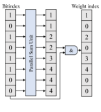
(b) Generate weights indices

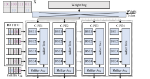
(c) The Combination Unit

Figure 10: Microarchitecture of the Combination Engine including a Decoder and a Combination Unit.

V-C Combination Engine

1) Decoder: As illustrated in Fig. 10(a), the Decoder is composed of a Package Division Unit and a Weight Index Generator, in which the goal of the Package Division Unit is to select valid values within the package, and the Weight Index Generator is responsible for calculating the row indices used to load weights. The Package Reg is a register used to cache the package from Input Buffer. First, the Package Division Unit extracts the Mode and Bitwidth from the Package Reg and feeds the non-zero values within the package to the Bit Selector. Next, the Bit Selector selects the valid bits using the corresponding selector, and then passes them to the Combination Unit for bit-serial computation. For example, when the Val Array of a package is $10,01,10,11$ and the quantization bitwidth is 2bit, the 2Bit Selector is used to select the valid bits as $1\underline{0},0\underline{1},1\underline{0},1\underline{1}$, and generates the pairs of feature bits and shift bit (0101,0 and 1011,1), which are fed to the Combination Unit to be processed in sequence. Shift bit is used to control the number of shifts in bit-serial computation. Since features in each package use the same bitwidth, the data format is fixed, which can substantially decrease the hardware complexity of the bit selectors. The Weight Index Generator parses the bitindex of node features in parallel by the Parallel Sum Unit to convert the bitindex to indices of the rows in $\mathbf{W}$, as shown in Fig. 10(b). Then these decoded weight indices are fed to the Combination Unit to load weights.

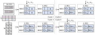
Figure 11: The cycle by cycle execution of two C-PEs, in which two BSEs process a group of two bits.

2) Combination Unit: The Combination Unit adopts the row-product manner and bit-serial computation approach to complete mixed-quantization calculation of $\mathbf{B=XW}$ ($\mathbf{X}$ is from 1 to 8bit). As shown in Fig. 10(c), a Combination Unit composes of a Bit FIFO, a Weight Reg, and $\#m$ Combination PEs (C-PEs). Node features from the Decoder are stored in the Bit FIFO and are subsequently loaded into the C-PEs in a bit-serial manner. The dense weights (quantized to 4bit) are buffered in the Weight Reg and are fetched to C-PEs via a crossbar according to the row indices from the Decoder. The C-PEs are responsible for the mixed-precision computation, and $\#m$ C-PEs can complete a Vector-Matrix multiplication between one row of $\mathbf{X}$ and $m$ columns of $\mathbf{W}$. Different C-PEs calculate different Vector-Vector multiplication to get $m$ different output features in the same row of $\mathbf{B}$. Each C-PE comprises of $\#n$ Bit-Serial Engines (BSEs), an Adder Tree, and a Shifter-Acc. Different BSEs complete the multiplication of different non-zero elements in the same row of $\mathbf{X}$ using corresponding weights. Since the bit-serial method greatly simplifies the multiplication operation, BSE only consists of an AND unit and three registers, including a weight register, a feature bit register, and a result register.

During processing, the C-PEs are equally divided into two groups, as illustrated in Fig. 10(c), and C-PEs in each group share the same features. The feature bits in the Bit FIFO are fed into the C-PEs for calculation and flow from the left half C-PE group to the right half for data reuse. Within each C-PE, BSEs execute AND operations between the feature bits and the loaded weights, with the results subsequently summarized in the Adder Tree. Then the sum is shifted according to the shift bit from the Decoder and accumulated with the partial sum until the final output is produced. In this way, the weights are reused across different bits of the node features. Given that the minimum bitwidth of the node features is 2bit in Degree-Aware method, each weight is reused at least twice, which reduces the weight bandwidth requirement of the C-PEs by half and also decreases the hardware complexity of the crossbar. Because the density of $\mathbf{W}$ is always 100%, the BSEs in the same row are all busy during the systolic process. A $c\times n(\frac{m}{2}\times 4\ \text{bits})$ crossbar is used to unicast corresponding rows of $W$ to C-PEs, where $c$ is the dimension of the feature slice processed in each Combination Tile.

Fig. 11 shows an example of the dataflow with m=2 and n=2. In the first cycle, the first feature bits and the corresponding weights are loaded to BSE1 and BSE2 of C-PE1. In the second cycle, BSE1 and BSE2 of C-PE1 perform the AND operations and load the second bits of the same non-zero values. The crossbar only loads weights to C-PE2, because the weights loaded to C-PE1 in the first cycle can be reused by the different bits of the same non-zero values. Moreover, the bits in C-PE1 are forwarded to C-PE2 for subsequent processing. The third and fourth cycles perform similarly.

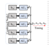
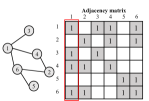
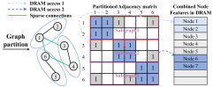
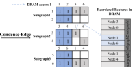
Figure 12: (a) Aggregate using Node1. (b) Baseline graph without partition. (c) DRAM access for aggregating Subgraph2 after partition. (d) DRAM access for aggregating Subgraph2 with the Condense-Edge scheduling strategy.

V-D Aggregation Engine

The Aggregation Engine is composed of an Encoder, a Condense Unit, and an Aggregation Tile. The Condense Unit is used to perform our Condense-Edge scheduling strategy (detailed in Section V-E). The Aggregation Tile contains multiple Aggregation Units (AUs), which can perform integer addition and multiplication of scalar. Considering the results (quantized to 4bit) from Combination Engine are node-by-node and nearly 100% dense, the Aggregation Engine calculates the $\mathbf{A}\mathbf{B}$ in an outer product manner to fully reuse the generated nodes features. Different dimensions of features in a node are unicasted to different AUs and multiplied with the corresponding edge weight of $\mathbf{A}$ broadcasted to each AU, which is stored in the Edge Buffer using the CSC format. As the example shown in Fig. 12 and 12, the combined Node1 is used to partially aggregate Node1, Node3, Node4, and Node6 in sequence. If the features of one node cannot occupy all units, free units can be assigned to aggregate other nodes. The multiplied results are added with 16bit partial sums buffered in Aggregation Buffer to complete the aggregation. When the aggregation for a node is complete, it is sent to the Encoder to be encoded to Adaptive-Package format.

The Encoder is composed of $\#m$ Quantization-Nonlinear (QN) units, which complete the quantization process of $\#m$ values using the scales from the Weight Buffer. Moreover, each QN unit performs the ReLU non-linear operation and generates a bitindex to identify whether the value is zero. The non-zero values are concatenated and stored in a package register as the Val Array in a package. To maximize memory efficiency, we adopt a greedy heuristic method where the package register continuously stores non-zero values in successive nodes until the maximum package length is reached or the node’s bitwidth changes. Then we select the appropriate Mode according to the bit length of the values in the package register. And the Mode and Bitwidth are assembled as the header information and the package is written back into the Input Buffer as the input of the combination phase of the next layer. The Encoder repeatedly performs the above process until the aggregation phase of the current layer completes.

Algorithm 1 Condense-Edge scheduling strategy

1: Initialize: $\mathbf{eID\_list=\{eID\_FIFO_{1},...,eID\_FIFO_{n}\}}$: container of the sparse connections $e\_IDs$ and $eID\_FIFO_{i}$ stores $e\_IDs$ of the $i$-th subgraph in ascending order; $\mathbf{Address\_list}$: stores the initial memory addresses of the Sparse Buffer corresponding to different subgraphs.

2: Outputs: None (reorder the nodes features)

3: Condense-Edge($x$, $nID$, $SubNum$):

4: Partition the graph using METIS and initialize $\mathbf{eID\_list}$. $subID=0$

5: Store $x$ into the Combination Buffer

6: while $subID<SubNum$ do

7:    $eID\_FIFO=eID\_list[subID]$

8:    if $eID\_FIFO[0]==nID$ then

9:       $eID\_FIFO.pop()${# invalid the $eID$ have matched}

10:       $ptr=Address\_list[subID]$ and store the node features $x$ into Sparse Buffer according to the $ptr$ {# reorder the nodes features in Sparse Buffer}

11:       Increment $ptr$ and $Address\_list[subID]=ptr$

12:       $subID=subID+1$ {# compare with the next subgraph}

13:    else

14:       $subID=subID+1$

15:    end if

16:    If the corresponding region of the Sparse Buffer is full, write the data back to DRAM and reinitialize the $ptr$.

17: end while

18: end

V-E Condense-Edge Scheduling Strategy

During aggregation, the extreme sparsity of $\mathbf{A}$ ruins the data locality and its large size results in a considerable amount of partial sums, which puts forward high demand on the capacity of the Aggregation Buffer. Therefore, to improve the data reuse and reduce the resource requirement, many modern GNN accelerators divide the graph into several subgraphs using METIS[1], and then perform the aggregation one subgraph after another [23, 61], as shown in Fig. 12. In this way, the Aggregation Buffer only stores the aggregated partial sums of the processing subgraph and the spatial locality in the subgraph (blue region in adjacency matrix) is significantly improved.

However, as our analysis in Section III-B, the pitfall for the partition is the more irregular sparse connections (grey region in the adjacency matrix of Fig. 12) between subgraphs, which engenders the bottleneck in advancing performance. As an example shown in Fig.12, when using the sparse connections to aggregate the nodes in Subgraph2, DRAM accesses are needed to read the features of Node1 (to aggregate Node3) and Node6 (to aggregate Node4). Assuming that the granularity of each DRAM access is 128B, i.e., a continuous memory region of two nodes where each node has 128-dimension features and is quantized to 4bit, then the access behavior is: Node1 miss$\rightarrow$Node1&2 loaded from DRAM$\rightarrow$Node6 miss $\rightarrow$Node6&7 loaded from DRAM, which requires two DRAM accesses and only half is utilized in each DRAM access. To alleviate the irregularity induced by sparse connections, we propose the Condense-Edge scheduling strategy.

MEGA also performs the aggregation phase one subgraph after another. The key idea of the Condense-Edge scheduling strategy is that when the Aggregation Engine performs aggregation of the first subgraph using the newly combined node, the Condense Unit simultaneously reorders the node features. Then, the features required by the sparse connections is stored continuously, which will be used to aggregate other subgraphs, significantly improving DRAM access utilization.

As shown in Algorithm 1, we first divide the graph into several subgraphs using METIS[1]. Since partition is performed offline, we can obtain the number of subgraphs $SubNum$ and sparse connection IDs ($eIDs$) of each subgraph in advance, e.g., 3 and 6 in Subgraph1, which are stored in the Edge Buffer. We initialize the $eID\_list$ using these IDs. The Sparse Buffer is divided into $SubNum$ regions and each region stores the nodes features used by sparse connections of one specific subgraph. The $\mathbf{Address\_list}$ is initialized by the initial addresses of these regions. Once the features $x$ of one node generate from the Combination Engine, we compare its ID $nID$ with $eIDs$ of different subgraphs. If there is a match, it implies that the node features will be utilized by this sparse connection, and thus we store $x$ into the region of Sparse Buffer assigned to the corresponding subgraph ($subID$) according to the address stored in $Address\_list$. We then update the address to ensure the continuity of nodes features in the Sparse Buffer (line 11). When multiple nodes within the same subgraph are all connected with a node $i$ through sparse connections, we only store node $i$ once because it can be reused by these nodes in the same subgraph.

To curtail the overhead of matching, we store $eIDs$ in ascending order and initially set all IDs to be valid. If the ID matches, we set this ID to be invalid (line 9). In this way, once the node is generated from the Combination Engine, we only need to compare with the first ID in each $eID\_FIFO$ instead of all IDs, which considerably reduces the matching overhead. Regardless of whether there is a match or not, the node features need to be written to the Combination Buffer to aggregate the nodes without sparse connections.

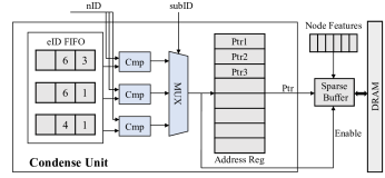
Figure 13: Microarchitecture of the Condense Unit.

When aggregating other subgraphs, the Sparse Buffer reads the nodes features used by sparse connections that have been continuously stored in DRAM. When features of one node is ready to be fetched to aggregate the nodes in the current subgraph, its $nID$ is compared with the $eIDs$. If there is a match, the Condense Unit directly fetches the required features from the Sparse Buffer. Otherwise, the needed node features are read from the Combination Buffer. As shown in Fig. 12, the access behavior of using sparse connections in Subgraph2 turns to: Node1 miss$\rightarrow$Node1 is used by the sparse connection$\rightarrow$Node1&6 loaded from DRAM to the Sparse Buffer$\rightarrow$Node6 match$\rightarrow$fetch Ndoe6 from the Sparse Buffer. Our Condense-Edge strategy reduces DRAM access from 2 to 1, improving the data reuse of each DRAM access.

Fig. 13 displays the microarchitecture of the Condense Unit. Each eID FIFO has eight entries and stores the $eIDs$ of a single subgraph, which are arranged in ascending order. Moreover, each eID FIFO is equipped with a comparator (Cmp) to improve the parallelism of matching.

VI Evaluation

VI-A Experiments Setup

1) Models and Datasets: We evaluate our framework on three GNN models - GCN[32], GIN[55], and GraphSage[20] using five datasets including three citation datasets (Cora, Cite, PubMed)[58], a knowledge graph dataset (NELL)[5], and a large scale dataset Reddit[20]. Details about datasets and models are shown in TABLE II and TABLE III, respectively.

2) Baselines: At the algorithm level, we compare our Degree-Aware quantization method with the FP32 models and the prior art method DQ[47] with 4bit (DQ-INT4) on various tasks. As node features dominate the memory consumption in GNNs, we count the average bitwidths for nodes features of the overall model and take the ratio of the average bitwidth / 32 as the theoretical compression ratio, named ‘CR’. At the hardware level, to evaluate our MEGA accelerator, we compare with four state-of-the-art architectures, i.e., HyGCN[56], GCNAX[36], GROW[23], and SGCN[60].

TABLE II: The statistics of datasets used in this work.

Dataset	#Node	#Edge	Feature length	Average degree
Cora	2,708	10,556	1,433	3.90
CiteSeer	3,327	9,104	3,703	2.74
PubMed	19,717	88,648	500	4.50
NELL	65,755	251,550	61,278	3.83
Reddit	232,965	114,615,892	602	491.99

TABLE III: The GNN models specifications.

Model	Sample nodes	Layers	Hidden units	Aggregation
GCN	—	2	128	Add
GIN	—	2	128	Add
GraphSage	25	2	256	Mean

3) Simulation: We use Verilog to implement MEGA and synthesize the RTL with Synopsys Design Compiler using the TSMC 28nm standard library at 1GHz to obtain area and power consumption of the processing units. For the SRAM-based on-chip buffers, we use CACTI-7.0[4] to model the area and power consumption. In TABLE IV, we give the configuration of MEGA and its breakdown analysis of area and power. We use HBM1.0[41] with 256GB/s bandwidth as the DRAM and model the off-chip access using Ramulator[31] and estimate the energy consumption for accessing DRAM following the methodology in [56].

TABLE IV: The configuration and breakdown of MEGA.

	Component	Area($mm^{2}$)	Power($mW$)	Config
Processing Unit	BSEs	0.053	14.70	$4\times 8\times 32$
	Aggregation Unit	0.100	28.92	256
	Crossbar	0.027	5.56	$32\times 8$(64bit)
	Condense Unit	0.002	1.19	16 ID FIFOs
	Encoder	0.010	1.81	32 QN units
	Decoder	0.003	0.75	—
	Others	0.004	0.80	—
Total		0.199(11%)	53.73(28%)	Size (KB)
Data Buffer	Aggregation Buffer	0.540	46.56	128
	Combination Buffer	0.452	35.19	96
	Input Buffer	0.220	22.88	64
	Edge Buffer	0.119	9.44	24
	Sparse Buffer	0.154	12.86	32
	Weight Buffer	0.190	14.32	48
Total		1.67(89%)	141.25(72%)	392
Measured Total(28nm)		1.869	194.98	—

TABLE V: The configurations of compared architectures.

Accelerator	Computing Unit@1GHz	Area($mm^{2}$)	Sparsity	Precision	Graph Partition
$\text{HyGCN}^{*}$	16 MACs 4 SIMD16	1.86	NO	32bits	No
GCNAX	32 MACs	1.85	Both Phases	32bits	No
$\text{SGCN}^{*}$	16 MACs 4 SIMD16	2.39	Aggregation Phase	32bits	No
GROW	32 MACs	2.36	Both Phases	32bits	Yes
MEGA	4x8x32 BSEs 256 Aggre Units	1.87	Both Phases	Mixed	Condense- Edge
* 16 MACs for combination and 4 SIMD16 for aggregation.

We implement cycle-accurate simulators of MEGA and the compared accelerators to simulate the behavior of the microarchitecture with the same DRAM bandwidth to obtain the number of cycles executed. The execution cycles of the computation modules of all simulators, including MEGA and all compared accelerators, have been validated with the HDL design at the cycle level. Given the significant configuration differences among compared accelerators, e.g., 22MB buffer size in HyGCN while 512KB in SGCN and a $32\times 128$ array in HyGCN while 16 MACs in GCNAX, we make the following efforts to ensure fair comparisons. First, we use the same on-chip buffer/cache capabilities (392KB) as MEGA. Second, for HyGCN and SGCN, which also employ a heterogeneous architecture, we match the OPS and convert the arithmetic operation to BitOP for consistency, with a 32bit fixed-point multiplication equivalent to 1024 BitOPs. Finally, for GCNAX and GROW adopting uniform computing units, we ensure the areas of their computing units to be comparable with the total area of the Processing Unit in our MEGA during simulation. More detailed configurations are listed in TABLE V.

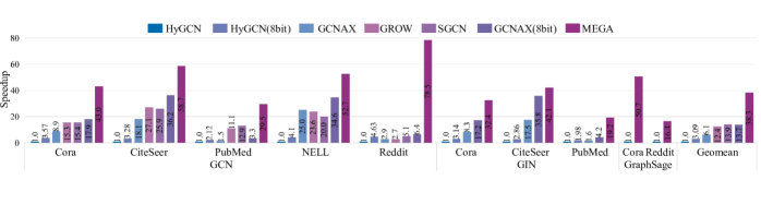
Figure 14: Performance comparison with state-of-the-art GNN accelerators (normalized to HyGCN).

TABLE VI: Comparisons with FP32 and DQ-INT4 models.

Dataset	Config	Acc	Average Bits	CR
Cora	GCN(FP32)	81.5±0.7%	32	1x
	GCN(DQ)	78.3±1.7%	4	8x
	GCN(ours)	80.9±0.6%	1.70	18.6x
	GIN(FP32)	77.6±1.1%	32	1x
	GIN(DQ)	69.9±3.4%	4	8x
	GIN(ours)	77.8±1.6%	2.37	13.4x
	GraphSage(FP32)	79.7±0.5%	32	1x
	GraphSage(Ours)	79.7±1.0%	3.40	9.4x
CiteSeer	GCN(FP32)	71.1±0.7%	32	1x
	GCN(DQ)	66.9±2.4%	4	8x
	GCN(Ours)	70.6±1.1%	1.87	17.0x
	GIN(FP32)	66.1±0.9%	32	1x
	GIN(DQ)	60.8±2.1%	4	8x
	GIN(ours)	65.1±1.7%	2.54	12.6x
PubMed	GCN(FP32)	78.9±0.7%	32	1x
	GCN(DQ)	62.5±2.4%	4	8x
	GCN(Ours)	78.3±0.6%	2.50	12.8x
Reddit	GraphSage(FP32)	95.2±0.1%	32	1x
	GraphSage(Ours)	95.6±0.2%	2.74	11.7x

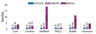
Figure 15: The performance comparison between accelerators using their original configurations and MEGA on GCN (normalized to GCNAX).

TABLE VII: The original configurations of compared architectures in a 28nm technology node.

Accelerator	Computing Unit@1GHz	On-chip Buffer(KB)	Area($mm^{2}$)	Power($mW$)
GCNAX	16 MACs	580	2.34	223.18
GROW	16 MACs	538	2.67	242.44

VI-B Accuracy

In TABLE VI, we present comparisons of the accuracy and compression ratio of our method with both FP32 models and DQ-INT4 models (denoted by ‘DQ’) on various tasks. Extensive experiments demonstrate that our approach can obtain a high compression ratio while maintaining accuracy. Compared with DQ-INT4, our method achieves significantly better accuracy on all tasks, even with a higher compression ratio. Furthermore, we obtain a compression ratio of up to $18.6\times$ over the FP32 model with negligible loss of accuracy.

We do not compare with DQ-INT8 because our Degree-Aware method is able to obtain comparable accuracy compared to DQ-INT8 with much higher compression ratios, e.g., DQ-INT8 achieves 71.0% with 8bit while Degree-Aware is 70.6% with 1.87bit on CiteSeer dataset of GCN model. Moreover, we can trade off accuracy with compression ratio by tuning down the penalty factor on the $L_{memory}$. For example, when we turn down the penalty factor, we can achieve 71.2% accuracy with 2.24bit, which is still much lower than 8bit.

VI-C Overall Results

1) Speedup: As shown in Fig. 14, MEGA on-average achieves $38.3\times$, $7.1\times$, $4.0\times$, $3.6\times$ speedup over HyGCN, GCNAX, GROW, and SGCN, respectively. By supporting the calculation and storage of mixed-precision features, MEGA significantly reduces the computation latency and DRAM communication, achieving substantial speedups compared to state-of-the-art accelerators. The speedup over HyGCN is particularly significant because HyGCN adopts the execution order of $\mathbf{(AX)W}$, which introduces a large number of additional MAC operations, and it does not utilize any sparsity in the node features, resulting in considerable redundant DRAM accesses. Compared to GCNAX, MEGA achieves a significant speedup thanks to the lower quantization bitwidth and fewer pipeline stalls induced by off-chip traffic. Although GROW and SGCN leverage the sparsity, MEGA also obtains significant speedup from the high compression ratio brought by our Degree-Aware method. To demonstrate the superiority of our MEGA, we also compare with the 8-bit version of HyGCN and GCNAX, which run GNNs quantized by DQ-INT8 using 8bit MACs, referred to as ‘HyGCN(8bit)’ and ‘GCNAX(8bit)’. We can observe that the improvement over their own 32-bit versions is marginal because the reduction on DRAM access of quantizing to 8bit is not sufficient for such a large number of irregular DRAM accesses in GNN workloads. On average, the dedicated MEGA significantly outperforms GCNAX(8bit) on performance by $2.8\times$, which identifies that naively replacing the computation units and running 8-bit quantized models on prior accelerators are sub-optimal.

As shown in Fig. 15, to present a more comprehensive comparison, we also compare MEGA with GCNAX and GROW that use their original configurations reported in corresponding papers. TABLE VII presents the original configurations of these compared accelerators. We do not provide the comparison with HyGCN and SGCN, which adopt much larger on-chip memory (e.g., 22MB v.s. 392KB) or many more computing units (e.g., 32$\times$128 32-bit MAC array v.s. 4$\times$8$\times$32 BSEs). With much smaller chip area and power, MEGA on-average obtains $4.68\times$ and $2.53\times$ performance over GCNAX and GROW, respectively, thanks to the significant reduction in DRAM accesses and computational latency brought by our software and hardware co-design framework.

2) DRAM access: As shown in Fig. 18, on average, MEGA achieves $108.1\times$, $10.5\times$, $8.4\times$, and $7.3\times$ reduction on DRAM access over HyGCN, GCNAX, GROW, and SGCN, respectively. The gains are mainly coming from two aspects: (i) Our Degree-Aware method obtains a high compression ratio at the algorithm level. (ii) Adaptive-Package format transfers the theoretical memory benefits into practical DRAM access reduction to the maximum extent and the Condense-Edge approach significantly improves data reuse and further decreases DRAM access. MEGA obtains significant DRAM access reduction over HyGCN because HyGCN neither uses graph partition to improve data locality nor utilizes the feature sparsity. While GROW consider the sparsity and adopt the partition algorithm to improve data locality, there remains considerable irregular DRAM accesses induced by the sparse connections, which is substantially alleviated by our Condense-Edge approach in MEGA.

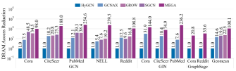
Figure 16: DRAM access reduction of MEGA and the baseline accelerators (normalized to HyGCN).

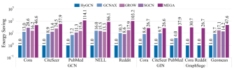
Figure 17: Energy savings of MEGA over the baseline accelerators (normalized to HyGCN).

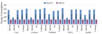
Figure 18: Energy consumption breakdown comparisons with HyGCN on GCN (normalized to our MEGA).

3) Energy saving: Fig. 18 demonstrates that our accelerator has a significant energy-efficiency superiority compared to other state-of-the-art accelerators. On average, our MEGA achieves $47.6\times$, $7.2\times$, $5.4\times$, $4.5\times$ energy savings compared to HyGCN, GCNAX, GROW, and SGCN, respectively. The energy efficiency gains are mainly attributed to the significant reduction of DRAM access brought by our Degree-Aware method and the innovative Adaptive-Package format. In addition, by supporting the mixed-precision computation, the low-bit integers are used for computation instead of float-point data, further reducing energy consumption. Fig. 18 displays a breakdown analysis of the energy consumption in HyGCN and MEGA when running GCN. The consumption is divided into four parts: DRAM, SRAM, Processing Unit (PU), and Leakage. As the results show, MEGA has significant energy savings on all four parts, especially on DRAM access.

VI-D Ablation Study

To analyze where our gains come from and demonstrate the effectiveness of our three proposed techniques separately, we conduct breakdown analysis on speedup and DRAM access.

1) Speedup: Fig. 19(a) illustrates the contribution of each proposed method towards the speedup improvement of MEGA compared to HyGCN-C, which also adopts the execution order of $\mathbf{A(XW)}$ to eliminate the contribution of the execution order in comparisons. When running the GCN quantized by our Degree-Aware method but in which the mixed-precision features are stored in Bitmap format, there is a significant performance improvement of $4.8\times$ speedup on average. Quantization not only decreases computational latency by using fixed-point operations, but also significantly decreases pipeline stall by reducing DRAM access. When our Adaptive-Package sparse format is supported, MEGA obtains an average speedup of $4.7\times$ compared with the Bitmap format. The gain is mainly from that Adaptive-Package can store mixed-precision features with their own quantization bitwidths rather than the highest bitwidth (8bit), which significantly reduces the latency of bit-serial computation and also decreases memory overhead. Applying the Condense-Edge scheduling strategy provides a further $1.1\times$ speedup, in which the contribution is not significant because most cycles of the DRAM accesses can be overlapped, especially for quantized models.

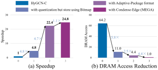
Figure 19: (a) The contribution of each method to the improvement of performance. (b) The contribution of each method to the DRAM access reduction.

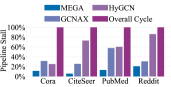
(a) Pipeline stall

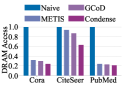
(b) DRAM access

Figure 20: (a) The comparisons of stall induced by DRAM access. (b) The superiority of our Condense-Edge.

2) DRAM access: The breakdown analysis in Fig. 19(b) demonstrates that our Degree-Aware quantization method is effective in decreasing DRAM access, which can be reduced by a factor of $5.8\times$ on average. Furthermore, when supporting the Adaptive-Package format, MEGA reduces the DRAM access by an average $2.5\times$. Our Condense-Edge scheduling strategy also significantly contributes to reducing DRAM access by an average $4.4\times$, especially on the graph with a more sparse adjacency matrix, e.g., NELL (0.0073%, $11.6\times$). Based on our three proposed techniques, MEGA substantially reduces the stalls induced by the DRAM access compared to HyGCN and GCNAX, as shown in Fig. 20(a).

The DRAM access comparison between our Condense-Edge method and other methods of enhancing the data locality is shown in Fig. 20(b). ‘Naive’ indicates that no method is used. ‘METIS’ denotes that divide the graph using METIS[1]. GCoD partitions the graph using METIS and prunes the sparse connections. The comparison shows that our approach is superior to other methods in reducing DRAM access.

VI-E Sensitivity Studies

1) The length settings in Adaptive-Package format. Since the three length settings in Adaptive-Package format are experimentally searched, we analyze the impacts of different settings on DRAM access, as shown in Fig. 21. We observe that the settings to achieve the optimal case are various for different datasets. For example, the optimal situation on PubMed is achieved by (400bits, 512bits, 800bits), in which the Cora and CiteSeer are much worse than their optimal cases. Considering the optimization across various datasets, we finally adopt the setting of (64, 128, 192) in our design.

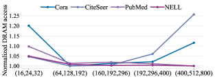
Figure 21: Design space exploration on the length settings of Adaptive-Package format (normalized to the optimal situation).

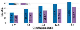
Figure 22: Sensitivity to the compression ratios on Cora of GCN and GIN (normalized to HyGCN).

2) Sensitivity on the compression ratio. As an accelerator that supports the storage and computation of mixed-precision node features, the compression ratio may significantly affect MEGA’s performance. Therefore, as illustrated in Fig. 22, we explore the sensitivity of MEGA’s performance to the compression ratio. We can observe that the performance of MEGA scales well with the increased compression ratio.

VII Discussion

1) The training overhead of Degree-Aware quantization method. We compare training time between FP32 models and quantized models on various datasets and GNN models. On average, the training time of quantized models is 2.04x over the FP32 models and the memory overhead is up to 12.8% on one 3090GPU. The training cost in both time and memory is acceptable. The training overhead of our method is much less than the state-of-the-art GNN quantization method DQ, which on-average costs 1.58x training time compared with ours.

2) The broader applicability of the Condense-Edge. The Condense-Edge method is initialized by partitioning graphs using METIS, which may become inefficient when processing dynamic or large-scale graphs. However, in such cases, our Condense-Edge method can work without partitioning while reaping comparable gains in speedup and energy efficiency. For instance, compared with the state-of-the-art accelerator SGCN, our MEGA without partitioning on-average obtains $3.50\times$ ($\downarrow$3% compared to MEGA using METIS) and $3.95\times$ ($\downarrow$14%) improvement on speedup and energy efficiency, respectively. This indicates that our Condense-Edge method works well without partitioning (just with a little performance discount) because the connections in the original graph are also extremely sparse, which is a challenge effectively addressed by the reorder process in our Condense-Edge method. Therefore, our Condense-Edge can be applied widely to various types of graphs, including dynamic or large-scale graphs.

3) The support of Graph Attention Network (GAT). With the same combination phase as GCN, GAT[50] employs the attention mechanism as its aggregation function, which involves MLP and softmax operators. Quantized by our Degree-Aware method, GAT obtains up to $16.5\times$ (from $9.6\times$) compression ratio with negligible accuracy loss (e.g., on CiteSeer, FP32: 72.5%, Degree-Aware: 71.9%). MLP can be computed reusing MEGA’s Combination Engine and there are multiple prior literature[19, 39, 45] on hardware-accelerated softmax, which can be directly integrated into MEGA with minor changes to the dataflow. For example, supporting GAT is estimated to incur a 1.5% area overhead using the hardware-accelerated softmax design in $A^{3}$[19].

VIII Conclusion

In this paper, we propose an algorithm and hardware co-design framework to boost the memory efficiency in GNN acceleration. Specifically, at the algorithm level, we propose the Degree-Aware mixed-precision quantization method, in which a proper bitwidth is learned and allocated to a node according to its in-degree to compress GNNs as much as possible while retaining accuracy. At the hardware level, we propose our MEGA accelerator adopting an innovative sparse format named Adaptive-Package to thoroughly transfer the theoretical gains on memory into an empirical improvement of performance and energy-efficiency. We also present a Condense-Edge scheduling strategy to alleviate the numerous and irregular DRAM accesses caused by the extremely sparse adjacency matrix. Extensive experiments at the algorithm and hardware levels demonstrate the superiority of our MEGA.

References

- [1] A. Abou-Rjeili and G. Karypis, “Multilevel algorithms for partitioning power-law graphs,” in Proceedings 20th IEEE International Parallel & Distributed Processing Symposium. IEEE, 2006, pp. 10–pp.
- [2] W. Aiello, F. Chung, and L. Lu, “A random graph model for power law graphs,” Experimental mathematics, vol. 10, no. 1, pp. 53–66, 2001.
- [3] M. Bahri, G. Bahl, and S. Zafeiriou, “Binary graph neural networks,” in Proceedings of the IEEE/CVF Conference on Computer Vision and Pattern Recognition, 2021, pp. 9492–9501.
- [4] R. Balasubramonian, A. B. Kahng, N. Muralimanohar, A. Shafiee, and V. Srinivas, “Cacti 7: New tools for interconnect exploration in innovative off-chip memories,” ACM Transactions on Architecture and Code Optimization (TACO), vol. 14, no. 2, pp. 1–25, 2017.
- [5] A. Carlson, J. Betteridge, B. Kisiel, B. Settles, E. Hruschka, and T. Mitchell, “Toward an architecture for never-ending language learning,” in Proceedings of the AAAI conference on artificial intelligence, vol. 24, no. 1, 2010, pp. 1306–1313.
- [6] C. Chen, K. Li, Y. Li, and X. Zou, “Regnn: A redundancy-eliminated graph neural networks accelerator,” in 2022 IEEE International Symposium on High-Performance Computer Architecture (HPCA). IEEE, 2022, pp. 429–443.
- [7] C. Chen, K. Li, X. Zou, and Y. Li, “Dygnn: Algorithm and architecture support of dynamic pruning for graph neural networks,” in 2021 58th ACM/IEEE Design Automation Conference (DAC). IEEE, 2021, pp. 1201–1206.
- [8] W. Chen, P. Wang, and J. Cheng, “Towards mixed-precision quantization of neural networks via constrained optimization,” in Proceedings of the IEEE/CVF International Conference on Computer Vision, 2021, pp. 5350–5359.
- [9] S. Dai, R. Venkatesan, M. Ren, B. Zimmer, W. Dally, and B. Khailany, “Vs-quant: Per-vector scaled quantization for accurate low-precision neural network inference,” Proceedings of Machine Learning and Systems, vol. 3, pp. 873–884, 2021.
- [10] Z. Dong, Z. Yao, D. Arfeen, A. Gholami, M. W. Mahoney, and K. Keutzer, “Hawq-v2: Hessian aware trace-weighted quantization of neural networks,” Advances in neural information processing systems, vol. 33, pp. 18 518–18 529, 2020.
- [11] Z. Dong, Z. Yao, A. Gholami, M. W. Mahoney, and K. Keutzer, “Hawq: Hessian aware quantization of neural networks with mixed-precision,” in Proceedings of the IEEE/CVF International Conference on Computer Vision, 2019, pp. 293–302.
- [12] A. Dosovitskiy, L. Beyer, A. Kolesnikov, D. Weissenborn, X. Zhai, T. Unterthiner, M. Dehghani, M. Minderer, G. Heigold, S. Gelly et al., “An image is worth 16x16 words: Transformers for image recognition at scale,” in International Conference on Learning Representations, 2020.
- [13] S. K. Esser, J. L. McKinstry, D. Bablani, R. Appuswamy, and D. S. Modha, “Learned step size quantization,” in International Conference on Learning Representations, 2020.
- [14] W. Fan, Y. Ma, Q. Li, Y. He, E. Zhao, J. Tang, and D. Yin, “Graph neural networks for social recommendation,” in The world wide web conference, 2019, pp. 417–426.
- [15] B. Feng, Y. Wang, X. Li, S. Yang, X. Peng, and Y. Ding, “Sgquant: Squeezing the last bit on graph neural networks with specialized quantization,” in 2020 IEEE 32nd International Conference on Tools with Artificial Intelligence (ICTAI). IEEE, 2020, pp. 1044–1052.
- [16] T. Geng, A. Li, R. Shi, C. Wu, T. Wang, Y. Li, P. Haghi, A. Tumeo, S. Che, S. Reinhardt et al., “Awb-gcn: A graph convolutional network accelerator with runtime workload rebalancing,” in 2020 53rd Annual IEEE/ACM International Symposium on Microarchitecture (MICRO). IEEE, 2020, pp. 922–936.
- [17] J. Gilmer, S. S. Schoenholz, P. F. Riley, O. Vinyals, and G. E. Dahl, “Neural message passing for quantum chemistry,” in International conference on machine learning. PMLR, 2017, pp. 1263–1272.
- [18] J. E. Gonzalez, Y. Low, H. Gu, D. Bickson, and C. Guestrin, “Powergraph: Distributed graph-parallel computation on natural graphs,” in Presented as part of the 10th USENIX Symposium on Operating Systems Design and Implementation (OSDI 12), 2012, pp. 17–30.
- [19] T. J. Ham, S. J. Jung, S. Kim, Y. H. Oh, Y. Park, Y. Song, J.-H. Park, S. Lee, K. Park, J. W. Lee et al., “A^ 3: Accelerating attention mechanisms in neural networks with approximation,” in 2020 IEEE International Symposium on High Performance Computer Architecture (HPCA). IEEE, 2020, pp. 328–341.
- [20] W. Hamilton, Z. Ying, and J. Leskovec, “Inductive representation learning on large graphs,” Advances in neural information processing systems, vol. 30, 2017.
- [21] S. Han, X. Liu, H. Mao, J. Pu, A. Pedram, M. A. Horowitz, and W. J. Dally, “Eie: Efficient inference engine on compressed deep neural network,” ACM SIGARCH Computer Architecture News, vol. 44, no. 3, pp. 243–254, 2016.
- [22] K. He, X. Zhang, S. Ren, and J. Sun, “Deep residual learning for image recognition,” in Proceedings of the IEEE conference on computer vision and pattern recognition, 2016, pp. 770–778.
- [23] R. Hwang, M. Kang, J. Lee, D. Kam, Y. Lee, and M. Rhu, “Grow: A row-stationary sparse-dense gemm accelerator for memory-efficient graph convolutional neural networks,” in 2023 IEEE International Symposium on High-Performance Computer Architecture (HPCA). IEEE, 2023, pp. 42–55.
- [24] S. Jain, A. Gural, M. Wu, and C. Dick, “Trained quantization thresholds for accurate and efficient fixed-point inference of deep neural networks,” Proceedings of Machine Learning and Systems, vol. 2, pp. 112–128, 2020.
- [25] B. Jin, C. Gao, X. He, D. Jin, and Y. Li, “Multi-behavior recommendation with graph convolutional networks,” in Proceedings of the 43rd International ACM SIGIR Conference on Research and Development in Information Retrieval, 2020, pp. 659–668.
- [26] Y. Jing, Y. Yang, X. Wang, M. Song, and D. Tao, “Meta-aggregator: Learning to aggregate for 1-bit graph neural networks,” in Proceedings of the IEEE/CVF International Conference on Computer Vision, 2021, pp. 5301–5310.
- [27] P. Judd, J. Albericio, T. Hetherington, T. M. Aamodt, and A. Moshovos, “Stripes: Bit-serial deep neural network computing,” in 2016 49th Annual IEEE/ACM International Symposium on Microarchitecture (MICRO). IEEE, 2016, pp. 1–12.
- [28] G. Karypis and V. Kumar, “A fast and high quality multilevel scheme for partitioning irregular graphs,” SIAM Journal on scientific Computing, vol. 20, no. 1, pp. 359–392, 1998.
- [29] J. D. M.-W. C. Kenton and L. K. Toutanova, “Bert: Pre-training of deep bidirectional transformers for language understanding,” in Proceedings of NAACL-HLT, 2019, pp. 4171–4186.
- [30] D. Kim, J. Ahn, and S. Yoo, “A novel zero weight/activation-aware hardware architecture of convolutional neural network,” in Design, Automation & Test in Europe Conference & Exhibition (DATE), 2017. IEEE, 2017, pp. 1462–1467.
- [31] Y. Kim, W. Yang, and O. Mutlu, “Ramulator: A fast and extensible dram simulator,” IEEE Computer architecture letters, vol. 15, no. 1, pp. 45–49, 2015.
- [32] T. N. Kipf and M. Welling, “Semi-supervised classification with graph convolutional networks,” in International Conference on Learning Representations, 2016.
- [33] M. Klimke, B. Völz, and M. Buchholz, “Cooperative behavior planning for automated driving using graph neural networks,” in 2022 IEEE Intelligent Vehicles Symposium (IV). IEEE, 2022, pp. 167–174.
- [34] A. Krizhevsky, I. Sutskever, and G. E. Hinton, “Imagenet classification with deep convolutional neural networks,” Communications of the ACM, vol. 60, no. 6, pp. 84–90, 2017.
- [35] A. Lerer, L. Wu, J. Shen, T. Lacroix, L. Wehrstedt, A. Bose, and A. Peysakhovich, “Pytorch-biggraph: A large scale graph embedding system,” Proceedings of Machine Learning and Systems, vol. 1, pp. 120–131, 2019.
- [36] J. Li, A. Louri, A. Karanth, and R. Bunescu, “Gcnax: A flexible and energy-efficient accelerator for graph convolutional neural networks,” in 2021 IEEE International Symposium on High-Performance Computer Architecture (HPCA). IEEE, 2021, pp. 775–788.
- [37] S. Liang, Y. Wang, C. Liu, L. He, L. Huawei, D. Xu, and X. Li, “Engn: A high-throughput and energy-efficient accelerator for large graph neural networks,” IEEE Transactions on Computers, vol. 70, no. 9, pp. 1511–1525, 2020.
- [38] Y.-C. Lin, B. Zhang, and V. Prasanna, “Hp-gnn: generating high throughput gnn training implementation on cpu-fpga heterogeneous platform,” in Proceedings of the 2022 ACM/SIGDA International Symposium on Field-Programmable Gate Arrays, 2022, pp. 123–133.
- [39] A. Marchisio, B. Bussolino, E. Salvati, M. Martina, G. Masera, and M. Shafique, “Enabling capsule networks at the edge through approximate softmax and squash operations,” in Proceedings of the ACM/IEEE International Symposium on Low Power Electronics and Design, 2022, pp. 1–6.
- [40] A. H. Nodehi Sabet, J. Qiu, and Z. Zhao, “Tigr: Transforming irregular graphs for gpu-friendly graph processing,” ACM SIGPLAN Notices, vol. 53, no. 2, pp. 622–636, 2018.
- [41] M. O’Connor, “Highlights of the high-bandwidth memory (hbm) standard,” in Memory Forum Workshop, vol. 3, 2014.
- [42] R. Sarkar, S. Abi-Karam, Y. He, L. Sathidevi, and C. Hao, “Flowgnn: A dataflow architecture for real-time workload-agnostic graph neural network inference,” in 2023 IEEE International Symposium on High-Performance Computer Architecture (HPCA). IEEE, 2023, pp. 1099–1112.
- [43] S. Sharify, A. D. Lascorz, M. Mahmoud, M. Nikolic, K. Siu, D. M. Stuart, Z. Poulos, and A. Moshovos, “Laconic deep learning inference acceleration,” in Proceedings of the 46th International Symposium on Computer Architecture, 2019, pp. 304–317.
- [44] H. Sharma, J. Park, N. Suda, L. Lai, B. Chau, V. Chandra, and H. Esmaeilzadeh, “Bit fusion: Bit-level dynamically composable architecture for accelerating deep neural network,” in 2018 ACM/IEEE 45th Annual International Symposium on Computer Architecture (ISCA). IEEE, 2018, pp. 764–775.
- [45] J. R. Stevens, R. Venkatesan, S. Dai, B. Khailany, and A. Raghunathan, “Softermax: Hardware/software co-design of an efficient softmax for transformers,” in 2021 58th ACM/IEEE Design Automation Conference (DAC). IEEE, 2021, pp. 469–474.
- [46] C. Szegedy, W. Liu, Y. Jia, P. Sermanet, S. Reed, D. Anguelov, D. Erhan, V. Vanhoucke, and A. Rabinovich, “Going deeper with convolutions,” in Proceedings of the IEEE conference on computer vision and pattern recognition, 2015, pp. 1–9.
- [47] S. A. Tailor, J. Fernandez-Marques, and N. D. Lane, “Degree-quant: Quantization-aware training for graph neural networks,” in International Conference on Learning Representations, 2020.
- [48] S. Uhlich, L. Mauch, F. Cardinaux, K. Yoshiyama, J. A. Garcia, S. Tiedemann, T. Kemp, and A. Nakamura, “Mixed precision dnns: All you need is a good parametrization,” in International Conference on Learning Representations, 2019.
- [49] A. Vaswani, N. Shazeer, N. Parmar, J. Uszkoreit, L. Jones, A. N. Gomez, Ł. Kaiser, and I. Polosukhin, “Attention is all you need,” Advances in neural information processing systems, vol. 30, 2017.
- [50] P. Veličković, G. Cucurull, A. Casanova, A. Romero, P. Liò, and Y. Bengio, “Graph attention networks,” in International Conference on Learning Representations, 2018.
- [51] H. Wang, D. Lian, Y. Zhang, L. Qin, X. He, Y. Lin, and X. Lin, “Binarized graph neural network,” World Wide Web, vol. 24, no. 3, pp. 825–848, 2021.
- [52] J. Wang, Y. Wang, Z. Yang, L. Yang, and Y. Guo, “Bi-gcn: Binary graph convolutional network,” in Proceedings of the IEEE/CVF Conference on Computer Vision and Pattern Recognition, 2021, pp. 1561–1570.
- [53] X. Weng, Y. Yuan, and K. Kitani, “Joint 3d tracking and forecasting with graph neural network and diversity sampling,” arXiv preprint arXiv:2003.07847, vol. 2, no. 6.2, p. 1, 2020.
- [54] C. Xie, L. Yan, W.-J. Li, and Z. Zhang, “Distributed power-law graph computing: Theoretical and empirical analysis,” Advances in neural information processing systems, vol. 27, 2014.
- [55] K. Xu, W. Hu, J. Leskovec, and S. Jegelka, “How powerful are graph neural networks?” in International Conference on Learning Representations, 2018.
- [56] M. Yan, L. Deng, X. Hu, L. Liang, Y. Feng, X. Ye, Z. Zhang, D. Fan, and Y. Xie, “Hygcn: A gcn accelerator with hybrid architecture,” in 2020 IEEE International Symposium on High Performance Computer Architecture (HPCA). IEEE, 2020, pp. 15–29.
- [57] M. Yan, X. Hu, S. Li, A. Basak, H. Li, X. Ma, I. Akgun, Y. Feng, P. Gu, L. Deng et al., “Alleviating irregularity in graph analytics acceleration: A hardware/software co-design approach,” in Proceedings of the 52nd Annual IEEE/ACM International Symposium on Microarchitecture, 2019, pp. 615–628.
- [58] Z. Yang, W. Cohen, and R. Salakhudinov, “Revisiting semi-supervised learning with graph embeddings,” in International conference on machine learning. PMLR, 2016, pp. 40–48.
- [59] Z. Yang and S. Dong, “Hagerec: Hierarchical attention graph convolutional network incorporating knowledge graph for explainable recommendation,” Knowledge-Based Systems, vol. 204, p. 106194, 2020.
- [60] M. Yoo, J. Song, J. Lee, N. Kim, Y. Kim, and J. Lee, “Sgcn: Exploiting compressed-sparse features in deep graph convolutional network accelerators,” in 2023 IEEE International Symposium on High-Performance Computer Architecture (HPCA). IEEE, 2023, pp. 1–14.
- [61] H. You, T. Geng, Y. Zhang, A. Li, and Y. Lin, “Gcod: Graph convolutional network acceleration via dedicated algorithm and accelerator co-design,” in 2022 IEEE International Symposium on High-Performance Computer Architecture (HPCA). IEEE, 2022, pp. 460–474.
- [62] H. Zeng and V. Prasanna, “Graphact: Accelerating gcn training on cpu-fpga heterogeneous platforms,” in proceedings of the 2020 ACM/SIGDA international symposium on field-programmable gate arrays, 2020, pp. 255–265.
- [63] S. Zhang, Z. Du, L. Zhang, H. Lan, S. Liu, L. Li, Q. Guo, T. Chen, and Y. Chen, “Cambricon-x: An accelerator for sparse neural networks,” in 2016 49th Annual IEEE/ACM International Symposium on Microarchitecture (MICRO). IEEE, 2016, pp. 1–12.
- [64] Z. Zhang, H. Wang, S. Han, and W. J. Dally, “Sparch: Efficient architecture for sparse matrix multiplication,” in 2020 IEEE International Symposium on High Performance Computer Architecture (HPCA). IEEE, 2020, pp. 261–274.
- [65] Y. Zhao, D. Wang, D. Bates, R. Mullins, M. Jamnik, and P. Lio, “Learned low precision graph neural networks,” arXiv preprint arXiv:2009.09232, 2020.