Comprehensive Quantum Calculation of the First Dielectric Virial Coefficient of Water

Abstract

We present a complete calculation, fully accounting for quantum effects and for molecular flexibility, of the first dielectric virial coefficient of water and its isotopologues. The contribution of the electronic polarizability is computed from a state-of-the-art intramolecular potential and polarizability surface from the literature, and its small temperature dependence is quantified. The dipolar polarizability is calculated in a similar manner with an accurate literature dipole-moment surface; it differs from the classical result both due to the different molecular geometries sampled at different temperatures and due to the quantization of rotation. We calculate the dipolar contribution independently from spectroscopic information in the HITRAN2020 database and find that the two methods yield consistent results. The resulting first dielectric virial coefficient provides a complete description of the dielectric constant at low density that can be used in humidity metrology and as a boundary condition for new formulations for the static dielectric constant of water and heavy water.

I Introduction

Water is crucial in many scientific and industrial contexts. Measurement of the water content of a gas (i.e., humidity) is needed in studies of the atmosphere related to weather and climate processes, but obtaining accurate, fast, and reproducible measurements is challenging. There are also industrial contexts where knowledge of water content is important; an example is natural gas transportation where water can freeze out as ice or form hydrates, both of which are undesirable and potentially dangerous.

One technology that has been proposed for humidity metrology is measurement of the static dielectric constant. Because the molecules in dry air (and, for the most part, in natural gas) are nonpolar, the presence of highly polar water molecules can have a significant effect on the dielectric constant, even at fairly low concentrations. Apparatus for measuring this effect has been developed by Cuccaro et al.[1] for water in air and nitrogen and by Gavioso et al.[2] for water in methane and natural gas. To apply such measurements in metrology, it is necessary to have an accurate expression for the contribution of water molecules to the static dielectric constant.

For a low-density gas with a dipole moment, the well-known classical relationship of the static dielectric constant $\varepsilon$ to the static isotropic electronic polarizability $\alpha$ and the squared magnitude of the molecular dipole moment $\mu^{2}$ of the gas constituent is given by the Debye–Langevin modification of the Clausius–Mossotti expression (CMDL):

$$\frac{\varepsilon-1}{\varepsilon+2}=\frac{4\pi}{3}N_{\mathrm{A}}\rho\left(\alpha+\frac{\mu^{2}}{3k_{\mathrm{B}}T}\right),$$ (1)

where $N_{\mathrm{A}}$ is the Avogadro constant, $\rho$ is the molar density, and $k_{\mathrm{B}}$ is the Boltzmann constant. The first dielectric virial coefficient $A_{\varepsilon}$ is defined as the low-density limit of the proportionality constant between the density and the Clausius–Mossotti quotient:

$$A_{\varepsilon}\equiv\lim_{\rho\to 0}\frac{1}{\rho}\frac{\varepsilon-1}{\varepsilon+2}.$$ (2)

For low-density gas mixtures, the left-hand side of Eq. (1) is simply the sum of $\rho A_{\varepsilon}$ of each pure component.

One might think that Eq. (1) provides a simple route to the calculation of $A_{\varepsilon}$ for water, and therefore to humidity metrology. The isotropic electronic polarizability of the water molecule in the ground rovibrational state has been calculated by ab initio quantum mechanics,[3] and the result is in good agreement with extrapolation of gas-phase refractivity measurements to the static limit.[4, 5] The dipole moment of the H₂O molecule in the rovibrational ground state has been measured to a relative uncertainty of $5\times 10^{-5}$.[6]

There are, however, several ways in which the classical Eq. (1) is oversimplified and slightly inaccurate. The purpose of this paper is to provide a rigorous accounting of all effects on $A_{\varepsilon}$, all of which involve quantum mechanics in one form or another.

First, the quantization of rotation means that the classical expression is inexact. A first-order correction for this quantum effect was first derived for rigid linear molecules by MacRury and Steele, [7] and was generalized to rigid nonlinear molecules by Gray et al.[8]

Second, molecules are not rigid objects, and hence the electronic polarizability has a small temperature dependence. Only at $0$ K does it assume the ground-state value; at higher temperatures other rovibrational states are occupied, each of which has a slightly different electronic polarizability.

Third, there is a similar effect for the dipole moment. The excited rovibrational states populated at finite temperatures have somewhat different dipole moments than the ground-state value. Additionally, the proper quantum mechanical derivation of the expression for the first dielectric virial coefficient shows that the generalizaton of Eq. (1) does not simply involve the average value of the dipole moment.

In this paper, we will discuss in detail how Eq. (1) is modified by quantum mechanical effects involving the rovibrational states of the water molecule. Additionally, we will provide the first fully quantum calculation of the first dielectric coefficient $A_{\varepsilon}$ of Eq. (2), discussing in detail the various quantum effects that one might expect for H₂O and its isotopologues due to their small moments of inertia and molecular flexibility.

II The first dielectric virial coefficient of a quantum polar molecule

The statistical derivation of the CMDL equation shows that the dielectric constant of a gas depends on the derivative of the polarization density $P(F)$ in an external electric field $F$ evaluated at zero field, [9, 8, 10]

$$\frac{\varepsilon-1}{\varepsilon+2}=\frac{4\pi}{3}\left.\frac{\mathrm{d}P(F)}{\mathrm{d}F}\right|_{F=0}\simeq A_{\varepsilon}\rho=\frac{4\pi}{3}\left.\frac{\mathrm{d}p(F)}{\mathrm{d}F}\right|_{F=0}~{}\rho N_{\mathrm{A}},$$ (3)

where in the right-hand side we have expanded $P(F)$ to first order as a function of the molar density $\rho$, [10] that is $P(F)=\rho N_{\mathrm{A}}p(F)$ where $p(F)$ is the dipole moment of an isolated molecule in the external field $F$. The quantity $A_{\varepsilon}$ is the first dielectric virial coefficient.

The dipole moment of a molecule in thermodynamic equilibrium at temperature $T$ in an electric field is given by the expectation value

$$p(F) = \frac{\mathrm{Tr}\left[(\mathbf{m}\cdot\mathbf{e}+\mathbf{e}\cdot\boldsymbol{\alpha}\cdot\mathbf{e}F)~{}\exp\left(-\beta H(F)\right)\right]}{\mathrm{Tr}\left[\mathrm{e}^{-\beta H(F)}\right]}$$ (4)

$$H(F) = H_{0}-F~{}\mathbf{m}\cdot\mathbf{e}-\frac{F^{2}}{2}~{}\mathbf{e}\cdot\boldsymbol{\alpha}\cdot\mathbf{e},$$ (5)

where $H_{0}$ is the Hamiltonian of the free molecule, $\beta=(k_{\mathrm{B}}T)^{-1}$, $\mathbf{e}$ is a unit vector in the direction of the externally applied electric field of magnitude $F$, $\boldsymbol{\alpha}$ is the molecular electronic polarizability tensor, and $\mathbf{m}$ is the molecular dipole moment. Notice that, in general, both the dipole moment $\mathbf{m}$ and the electronic polarizability tensor $\boldsymbol{\alpha}$ depend on the specific molecular orientation and configuration which, in the case of water, is determined by 6 degrees of freedom. Usually, these are given by three Euler angles defining the relation between the molecule-fixed and the the laboratory-fixed coordinate system, [11] the lengths $r_{1}$ and $r_{2}$ of the two O–H bonds, and the angle $\theta$ between their directions. The denominator in Eq. (4) is the partition function of a single molecule, and will be denoted by $Q_{1}(\beta,F)$.

II.1 Classical and semiclassical limit for rigid rotors

The evaluation of the derivative at zero external field appearing in equations (3), (4), and (5) can be performed explicitly. Its derivation is reported in the Supplementary Material and it shows that, in general, the first dielectric virial coefficient has two contributions,

$$A_{\varepsilon}=\frac{4\pi}{3}N_{\mathrm{A}}\left(\alpha_{\mathrm{el}}+\alpha_{\mathrm{dip}}\right),$$ (6)

where the first depends on the electronic polarizability surface $\boldsymbol{\alpha}$, while the second depends on the dipole-moment surface $\mathbf{m}$. In the classical limit, one recovers Eq. (1)

$$A_{\varepsilon}^{\mathrm{(cl)}}=\frac{4\pi}{3}N_{\mathrm{A}}\left\langle\alpha_{\mathrm{el}}+\frac{\beta|\mathbf{m}|^{2}}{3}\right\rangle,$$ (7)

where the average $\langle\cdots\rangle$ is over the internal configurations of the molecule; this is the result quoted in Ref. 7 and shows how to interpret the quantities $\alpha$ and $\mu^{2}$ in Eq. (1), which are the values of the electronic polarizability and the squared magnitude of the dipole moment at the assumed rigid configuration of water. In a simple classical rigid model of water (e.g., when the bond lengths $r_{1}$ and $r_{2}$ and the angle $\theta$ are fixed at their ground-state values [12]), the contribution to $A_{\varepsilon}$ from the dipole moment is $A_{\varepsilon}^{(\mathrm{dip,cl})}\sim 70.2$ cm³/mol at $T=300$ K, whereas that from the electronic polarizability tensor is on the order of $A_{\varepsilon}^{(\mathrm{el,cl})}\sim 3.7$ cm³/mol.

Semiclassical corrections to the dipolar contribution in Eq. (7) have been derived in Ref. 8, and are given by

$$\frac{\Delta A_{\varepsilon}^{\mathrm{(dip,semi)}}}{A_{\varepsilon}^{\mathrm{(dip,cl)}}}=\\ -\frac{\beta\hbar^{2}}{12|\mathbf{m}|^{2}}\left(\frac{m_{y}^{2}+m_{z}^{2}}{I_{x}}+\frac{m_{z}^{2}+m_{x}^{2}}{I_{y}}+\frac{m_{x}^{2}+m_{y}^{2}}{I_{z}}\right),$$ (8)

where $I_{i}$ are the principal moments of inertia of the molecule and $m_{i}$ are the components of the dipole moment along the principal axis. For water at $300$ K, the semiclassical correction of Eq. (8) is $A_{\varepsilon}^{\mathrm{(semi)}}=-2.0$ cm³/mol, which in relative terms is roughly 3% of the dipolar contribution.

II.2 Quantum statistics

In the general case, one has to be careful in performing the derivative with respect to $F$ in Eq. (3), due to the presence of non-commuting operators. Denoting by $|i\rangle$ a complete set of molecular rovibrational quantum states and by $E_{i}$ the corresponding energies, the fully quantum expressions for the two terms in Eq. (6) are (see the Supplementary Material for the derivation)

$$\alpha_{\mathrm{el}}(T) = \frac{1}{Q_{1}(\beta,0)}\sum_{i}\frac{\langle i|\mathrm{Tr}(\boldsymbol{\alpha})|i\rangle}{3}~{}\mathrm{e}^{-\beta E_{i}},$$ (9)

$$\alpha_{\mathrm{dip}}(T) = \frac{1}{Q_{1}(\beta,0)}\sum_{i\neq j}|\langle i|\mathbf{m}\cdot\mathbf{e}|j\rangle|^{2}\frac{\mathrm{e}^{-\beta E_{i}}-\mathrm{e}^{-\beta E_{j}}}{E_{j}-E_{i}}.$$ (10)

The quantum mechanical formula for $\alpha_{\mathrm{dip}}$ was first derived by Illinger and Smyth. [13] In general, a molecular eigenstate $|i\rangle$ is characterized by a set of rotational and vibrational quantum numbers and hence one can split the sum in Eq. (10) into two contributions: the first corresponds to those $i\leftrightarrow j$ transitions where the vibrational state changes, resulting in the so-called vibrational polarizability. The sum over the remaining transitions, which have the same vibrational quantum numbers, is called the rotational polarizability. [14]

In the $T\to 0$ limit, the electronic polarizability (9) becomes just an average over the ground rovibrational state $|0\rangle$, that is

$$\alpha_{\mathrm{el}}^{0}=\frac{1}{3}\langle 0|\mathrm{Tr}(\boldsymbol{\alpha})|0\rangle,$$ (11)

whereas the dipolar polarizability becomes [14]

$$\alpha_{\mathrm{dip}}^{0}=2\sum_{j\neq 0}\frac{|\langle 0|\mathbf{m}\cdot\mathbf{e}|j\rangle|^{2}}{E_{j}-E_{0}}=\frac{2}{3}\sum_{j\neq 0}\frac{|\langle 0|\mathbf{m}|j\rangle|^{2}}{E_{j}-E_{0}},$$ (12)

where we have used rotational invariance to substitute $\mathbf{e}\cdot\boldsymbol{\alpha}\cdot\mathbf{e}=\mathrm{Tr}(\boldsymbol{\alpha})/3$ and $|\langle i|\mathbf{m}\cdot\mathbf{e}|j\rangle|^{2}=|\langle i|\mathbf{m}|j\rangle|^{2}/3$.

In the high-temperature (classical) limit, $T\to\infty$, one can write

$$\mathrm{e}^{-\beta E_{i}}-\mathrm{e}^{-\beta E_{j}}\simeq\mathrm{e}^{-\beta E_{i}}\beta(E_{j}-E_{i}),$$ (13)

and Eq. (10) becomes

$$\alpha_{\mathrm{dip}}^{\mathrm{class}}(T)=\frac{\beta}{3}\frac{\sum_{i}\langle i||\mathbf{m}|^{2}|i\rangle\mathrm{e}^{-\beta E_{i}}}{Q_{1}(\beta,0)},$$ (14)

which can be seen as a generalization of the classical expression (7) where the square of the permanent dipole is replaced by its quantum thermal average, which depends only on the diagonal matrix elements of the corresponding operator. In general, however, the dipolar contribution to the first dielectric virial coefficient depends on all the matrix elements of the dipole moment, as evidenced by Eq. (10).

III Dipolar polarizability from spectroscopy

The dipolar polarizability (10) depends on the squared matrix elements of the dipole operator $\mathbf{m}$, which is the same operator that determines the Einstein coefficient associated with an electromagnetic transition between states of energy $E_{i}$ and $E_{j}$. [15] These coefficients, or equivalently the line intensities, of several thousands of transitions are available in the HITRAN2020 database [16] for many water isotopologues, as well as other molecules. This paves the way to an experimental determination of the dipolar polarizability from spectroscopic data.

To this end, let us rewrite Eq. (10) according to the following considerations: first of all, we notice that the quantity to be summed is invariant under the exchange $i\leftrightarrow j$. Hence, the dipolar polarizability is given by twice the sum performed over those states for which $E_{j}>E_{i}$. Second, there might be degeneracies among the energy levels, so let us denote by $d_{i}$ the number of states having energy $E_{i}$; in the case of water $d_{i}=(2J+1)g_{i}$ where $J$ is the angular momentum of state $i$ and $g_{i}$ is its nuclear-spin degeneracy. A general state $|i\rangle$ can then be labeled by its energy $E_{i}$ and an integer number $\xi$ running between $1$ and $d_{i}$. Finally, let us define the average dipole matrix element squared between levels with energy $E_{i}$ and $E_{j}$ as

$$M_{ij}=\frac{1}{d_{i}d_{j}}\sum_{\xi=1}^{d_{i}}\sum_{\eta=1}^{d_{j}}|\langle E_{i},\xi|\mathbf{m}\cdot\mathbf{e}|E_{j},\eta\rangle|^{2},$$ (15)

and the transition frequency $\omega_{ij}=(E_{j}-E_{i})/\hbar$. With these definitions, we can write the dipolar polarizability as

$$\alpha_{\mathrm{dip}}(T)=\frac{2}{Q_{1}(\beta)}\sum_{E_{j}>E_{i}}\frac{d_{i}d_{j}M_{ij}}{\hbar\omega_{ij}}\mathrm{e}^{-\beta E_{i}}\left(1-\mathrm{e}^{-\beta\hbar\omega_{ij}}\right).$$ (16)

On the other hand, the spectral line intensities $S_{ij}$ for the transitions between molecular levels of energy $E_{i}$ and $E_{j}$ reported in the HITRAN2020 database are given by (in our notation) [17, 18]

$$S_{ij}=\frac{2\pi}{\hbar c}I_{A}\omega_{ij}d_{i}d_{j}M_{ij}\frac{\mathrm{e}^{-\beta_{\mathrm{R}}E_{i}}(1-\mathrm{e}^{-\beta_{\mathrm{R}}\hbar\omega_{ij}})}{Q_{1}(\beta_{\mathrm{R}})},$$ (17)

where $I_{A}$ is the isotopic abundance of the species under consideration, $\beta_{\mathrm{R}}=(k_{\mathrm{B}}T_{\mathrm{R}})^{-1}$, and $T_{\mathrm{R}}=296$ K is a reference temperature. Consequently, one can write

$$\alpha_{\mathrm{dip}}(T) = \frac{c}{\pi~{}I_{A}}\sum_{E_{j}>E_{i}}\frac{S_{ij}}{\omega_{ij}^{2}}\frac{Q_{1}(\beta_{\mathrm{R}})}{\mathrm{e}^{-\beta_{\mathrm{R}}E_{i}}(1-\mathrm{e}^{-\beta_{\mathrm{R}}\hbar\omega_{ij}})}\times$$ (18)

$$\frac{\mathrm{e}^{-\beta E_{i}}(1-\mathrm{e}^{-\beta\hbar\omega_{ij}})}{Q_{1}(\beta)},$$

which enables the calculation of the dipolar polarizability based on the quantities $S_{ij}$, $\omega_{ij}$, $E_{i}$, $Q_{1}(\beta)$, that are all reported the HITRAN2020 database. Since the HITRAN2020 database also reports quantum numbers for the upper and lower states of the transitions, the calculation of the vibrational and rotational contributions to the dipolar polarizability using Eq. (18) is straightforward.

The HITRAN2020 database also reports the uncertainty associated with the line intensities $S_{ij}$; we have used this information to propagate it to the uncertainty of $A_{\varepsilon}^{\mathrm{(dip)}}$ using Eq. (18). In those cases where HITRAN2020 reported a range for the uncertainty, we made the conservative choice of taking the highest value and considering it to be a standard uncertainty.

IV Ab initio calculation of the first dielectric virial coefficient

The quantities $\alpha_{\mathrm{el}}(T)$ and $\alpha_{\mathrm{dip}}(T)$ can be computed from the knowledge of the intramolecular potential, the trace of the polarizability $\alpha(\mathbf{X})=\mathrm{Tr}(\boldsymbol{\alpha})$, and the dipole moment $\mathbf{m}(\mathbf{X})$, where $\mathbf{X}$ denotes a set of intramolecular coordinates (e.g., the two bond lengths and the HOH angle). All of these quantities are available from ab initio electronic structure calculations. In particular, we used the recent PES15K [19] potential-energy surface to compute the intramolecular potential, the dipole-moment surface $\mathbf{m}(\mathbf{X})$ CKAPTEN from Ref. 20, and the isotropic electronic polarizability $\alpha(\mathbf{X})$ from Ref. 3. In Ref. 3, the authors provide a fitting function based on extensive calculations of the polarizability for many molecular configurations (the DPS-H₂O-3K database), solving the electronic structure at the CCSDT/daTZ level of theory. In addition, they perfomed a few evaluations of the polarizability surface at a more accurate level of theory (CCSDT/daQZ + $\Delta\alpha_{\mathrm{basis}}$ + $\Delta\alpha_{\mathrm{core}}$). The values obtained in this case are much more accurate for configurations close to the equilibrium configuration of water. Therefore, we slightly changed their parametrization of the polarizability surface (from their Table II [3]) in order to obtain more accurate values around the equilibrium geometry. In practice, we changed the first line of their Table II (corresponding to $(ijk)=(000)$) to the values reported in their Table III, that is $\alpha_{xx}=9.8744$, $\alpha_{yy}=9.2233$, and $\alpha_{zz}=9.5190$ (in atomic units). This corresponds to a rigid shift of the isotropic part of the CKAPTEN polarizability surface by $\Delta\alpha_{\mathrm{iso}}=-0.039133$ atomic units, which in relative terms is approximately 0.4%.

There are two main ways to compute the first dielectric virial coefficient for water. The first is to diagonalize the Schrödinger equation for the nuclear motion of the water molecule, compute the temperature-dependent electronic polarizability of Eq. (9) and the dipolar polarizability of Eq. (10), and obtain the first dielectic virial coefficient from Eq. (6). Although there are efficient approaches to solve the quantum-mechanical three-body problem and obtain the rovibrational eigenstates of water molecules, a complete diagonalization of the intramolecular Hamiltonian becomes progressively more difficult for molecules with a larger number of atoms. We will show in the following how the two temperature-dependent contributions to $A_{\varepsilon}(T)$ can be obtained from a path-integral approach, which has a much more favorable computational scaling for polyatomic molecules.

IV.1 The discrete variable representation approach

In the case of water or other triatomic molecules, it is convenient to use the form of the three-body Hamiltonian in the molecule-fixed frame derived by Sutcliffe and Tennyson using Jacobi coordinates. [21] In this approach, one obtains, for each value of the total molecular angular momentum $J$, a vibrational Hamiltonian that depends on three coordinates: the moduli of the two Jacobi vectors, $R_{1}$ and $R_{2}$, and the value of the angle between them, $\Theta$. The full rovibrational spectrum of water can be obtained by diagonalizing the vibrational Hamiltonian for progressively larger values of the molecular angular momentum $J$. The Hamiltonian is conveniently written using the so-called Discrete Variable Representation (DVR), [22, 23, 24] which has been used in many investigations of water properties. [25, 26]

In practice, the rovibrational wavefunction is written as

$$\Psi_{J\nu mI}(q,\Omega,I)=\\ \sqrt{\frac{2J+1}{8\pi^{2}}}\sum_{k=-J}^{J}\psi_{J\nu}(q,k)D^{J}_{mk}(\Omega)\chi({\cal I}_{J\nu},I),$$ (19)

where $q=(R_{1},R_{2},\Theta)$ denotes the molecular vibrational coordinates, $\psi_{J\nu}(q,k)$ are the eigenfunctions of the rovibrational Hamiltonian in the molecule-fixed frame for a given value of $J$, $D^{J}_{mk}(\Omega)$ are Wigner rotation matrices from the molecule-fixed to the laboratory-fixed frames, and $\chi({\cal I}_{J\nu},I)$ denotes the wavefunction of nuclear spins, with total spin ${\cal I}_{J\nu}$ and projection $I$ along the laboratory $Z$ axis. In the case of water molecules with two identical hydrogen isotopes, the overall wavefunction in Eq. (19) must have a specific symmetry upon exchange of the two hydrogens, reflecting their fermionic (H or T, antisymmetric wavefunction) or bosonic (D, symmetric wavefunction) nature. The need of a well-defined exchange symmetry for the total wavefunction implies that the nuclear-spin state of the two hydrogens depends on exchange symmetry of the rovibrational state $\psi_{J\nu}$.

In the case of two hydrogen atoms (with nuclear spin $1/2$), molecular configurations have either ${\cal I}_{J\nu}=0$ (para-water) or ${\cal I}_{J\nu}=1$ (ortho-water), with multiplicities $g_{\mathrm{para}}=1$ and $g_{\mathrm{ortho}}=3$, respectively. In the case of two deuterium atoms (with nuclear spin $1$), the ortho spin isomer has total spin ${\cal I}$ which is either 0 or 2 (that is, degeneracy $g_{\mathrm{ortho}}=6$) or total spin $1$, with degeneracy $g_{\mathrm{para}}=3$. For the sake of completeness, we recall that nuclear spin degeneracies can also come from the oxygen spin, although in this case they do not depend on the rovibrational state. This is particularly relevant for the ¹⁷O oxygen isotope, which has ${\cal I}=5/2$. The other oxygen isotopes have ${\cal I}=0$.

Notice that the energy levels on the molecular Hamiltonian depend only on the quantum numbers $J$ (the total angular momentum), $k$ (the projection of the angular momentum in the molecule-fixed $z$ axis), and $\nu$ (that labels the vibrational states obtained for given values of $J$ and $k$). Rotational invariance implies a $2J+1$ degeneracy on the label $m$ in Eq. (19).

Evaluating the symmetry upon exchange of the wavefunctions $\psi_{J\nu k}(q)$, and hence the degeneracy, is a non-trivial procedure, [27] but this information is already included in the HITRAN2020 database. Given the accuracy of our calculated energy levels, we assigned degeneracies by looking at that of the closest energy level, for a given $J$, among the states present in HITRAN2020. Using the DVR approach, one can compute the electronic and dipolar contribution to the polarizability directly from the quantum mechanical expressions of Eqs. (9) and (10), respectively. In the first case, one obtains

$$\alpha_{\mathrm{el}}(T)=\sum_{J\nu}\frac{g_{J\nu}(2J+1)\mathrm{e}^{-\beta E_{J\nu}}}{3~{}Q_{1}(\beta,0)}\left\langle\psi_{J\nu}|\mathrm{Tr}(\boldsymbol{\alpha})|\psi_{J\nu}\right\rangle,$$ (20)

where $g_{J\nu}$ is the degeneracy of the given rovibrational state and, in the DVR representation, one has

$$\left\langle\psi_{J\nu}|\mathrm{Tr}(\boldsymbol{\alpha})|\psi_{J\nu}\right\rangle=\sum_{q,k}\left|\psi_{J\nu k}(q)\right|^{2}\mathrm{Tr}(\boldsymbol{\alpha}(q)),$$ (21)

since the trace of the polarizability tensor $\boldsymbol{\alpha}(q)$ is a scalar quantity and a diagonal operator in the DVR representation. Notice that in the case of a rigid model of water, the electronic polarizability (20) does not depend on temperature.

The quantum mechanical expression for $\alpha_{\mathrm{dip}}(T)$ is more complicated, because one needs to evaluate the matrix element of the components of the dipole moment $\mathbf{m}$ in the laboratory-fixed frame using wavefunctions defined in the molecule-fixed frame. [28, 11, 25] Its derivation is discussed in Appendix A, for both rigid and flexible molecular models.

IV.2 The path-integral approach

A first-principles evaluation of the first dielectric virial coefficient from Eqs. (3)–(5) can also be performed using the path-integral formulation of quantum statistical mechanics. [29] The main advantage of this method is that it works directly in the Cartesian coordinates of all the atoms, and hence one does not need the analytically complicated procedure of separating the center-of-mass, rotational, and vibrational motion as needed for solving the Schrödinger equation.

IV.2.1 Quantum rigid rotors

In the case of a rigid rotor, $\alpha_{\mathrm{el}}$ is a constant and hence easily evaluated. Taking the derivative with respect to $F$ of the first term in Eq. (3) requires some care, because the dipole moment direction in the laboratory reference frame, $\mathbf{m}\cdot\mathbf{e}$ (which will be denoted by $m_{Z}$ in the following), does not commute with $H_{0}$ which, in this case, is the Hamiltonian of a quantum asymmetric rigid rotor. It is convenient to specialize the trace as an integration over all possible orientations of the molecule – which will be denoted by $\Omega_{1}$ – and at the same time use Trotter’s identity to write

$$\mathrm{e}^{-\beta H_{0}+\beta\mathbf{m}\cdot\mathbf{e}F}\sim\left(\mathrm{e}^{-\beta H_{0}/P}\mathrm{e}^{\beta(\mathbf{m}\cdot\mathbf{e})F/P}\right)^{P},$$ (22)

which becomes an equality for a sufficiently large $P$. Inserting $P-1$ completeness relations of the form

$$1=\int|\Omega_{k}\rangle\langle\Omega_{k}|~{}\mathrm{d}\Omega_{k},$$

between the $P$ products in Eq. (22), one ends up with the expression

$$A_{\varepsilon} = \frac{4\pi}{3}\alpha_{\mathrm{el}}+\frac{4\pi}{3Q_{1}}\frac{\partial}{\partial F}\int m_{Z}(\Omega_{1})\prod_{k=1}^{P}\langle\Omega_{k}|\mathrm{e}^{-\beta H_{0}/P}|\Omega_{k+1}\rangle~{}\mathrm{e}^{\beta m_{Z}(\Omega_{k+1})F/P}\prod_{k=1}^{P}\mathrm{d}\Omega_{k}$$ (23)

$$= \frac{4\pi}{3}\alpha_{\mathrm{el}}+\frac{4\pi}{3Q_{1}}\int m_{Z}(\Omega_{1})\prod_{k=1}^{P}\langle\Omega_{k}|\mathrm{e}^{-\beta H_{0}/P}|\Omega_{k+1}\rangle~{}\left[\frac{\beta}{P}\sum_{k=1}^{P}m_{Z}(\Omega_{k})\right]~{}\prod_{k=1}^{P}\mathrm{d}\Omega_{k}$$ (24)

$$= \frac{4\pi}{3}\alpha_{\mathrm{el}}+\frac{4\pi\beta}{3Q_{1}}\int\prod_{k=1}^{P}\langle\Omega_{k}|\mathrm{e}^{-\beta H_{0}/P}|\Omega_{k+1}\rangle~{}\left[\frac{1}{P}\sum_{k=1}^{P}m_{Z}(\Omega_{k})\right]^{2}~{}\prod_{k=1}^{P}\mathrm{d}\Omega_{k},$$ (25)

$$= \frac{4\pi}{3}\alpha_{\mathrm{el}}+\frac{4\pi\beta}{9}\left\langle|\overline{\mathbf{m}}|^{2}\right\rangle,$$ (26)

where we have defined $\overline{\mathbf{m}}=\sum_{k}\mathbf{m}(\Omega_{k})/P$. In passing from (24) to (25), we have used the fact that singling out $m_{Z}(\Omega_{1})$ in (23) is an arbitrary choice that we have averaged upon. Notice also that we have defined $\Omega_{P+1}=\Omega_{1}$. The evaluation of the matrix elements $\langle\Omega_{k}|\mathrm{e}^{-\beta H_{0}/P}|\Omega_{k+1}\rangle$ for a rigid-rotor molecule is discussed in Refs. 30, 31.

IV.2.2 Quantum flexible molecules

In dealing with flexible models of water, it is convenient to denote by $\mathbf{X}$ the set of all the coordinates of the three atoms. In this case, $A_{\varepsilon}$ is still given by Eq. (3) where the Hamiltonian $H_{0}$ includes the kinetic energy of the three atoms, $K$, and the intramolecular potential $V_{\mathrm{int}}(\mathbf{X})$. Note that both the dipole moment $\mathbf{m}$ and the electronic polarizability tensor $\boldsymbol{\alpha}$ depend on $\mathbf{X}$. The path-integral evaluation of quantities related to flexible molecules has been described in detail in Ref. 32. The main result is that one can map the quantum partition function to a classical partition function where each atom is represented by a ring polymer with $P$ beads. This approach provides an explicit expression of the interaction between consecutive beads (that turns out to be an harmonic potential) and the interaction among the ring polymers, which depends on $V_{\mathrm{int}}(\mathbf{X})$. In the case of H₂O or D₂O, one has to consider the indistinguishability between the hydrogen or deuterium atoms within a molecule. Although this can be done in the path-integral approach, it can be shown that exchange effects are important only for temperatures $T\lesssim 50$ K [32] and therefore they will be neglected in this paper.

With a derivation analogous to that performed in the case of rigid rotors, the path-integral expression for $A_{\varepsilon}$ in the case of a flexible model turns out to be

$$A_{\varepsilon} = \frac{4\pi}{3}\int\left(\overline{\alpha_{\mathrm{el}}}+\frac{\beta}{3}\left|\overline{\mathbf{m}}\right|^{2}\right)\times$$ (27)

$${\cal P}(\mathbf{X}_{1},\ldots,\mathbf{X}_{P})\prod_{k=1}^{P}\mathrm{d}\mathbf{X}_{k}$$

$$\overline{\alpha_{\mathrm{el}}} = \frac{1}{P}\sum_{k=1}^{P}\alpha_{\mathrm{el}}(\mathbf{X}_{k})$$ (28)

$$\overline{\mathbf{m}} = \frac{1}{P}\sum_{k=1}^{P}\mathbf{m}(\mathbf{X}_{k})$$ (29)

$${\cal P}(\mathbf{X}_{1},\ldots,\mathbf{X}_{P}) = \frac{1}{Q_{1}}\prod_{k=1}^{P}\langle\mathbf{X}_{k}|\mathrm{e}^{-\beta T}|\mathbf{X}_{k+1}\rangle\times$$ (30)

$$\exp\left(-\frac{\beta}{P}\sum_{k=1}^{P}V_{\mathrm{int}}(\mathbf{X}_{k})\right),$$

where ${\cal P}(\cdots)$ is the probability of finding a specific molecular configuration in the path-integral representation.

The first term in Eq. (27) is the path-integral representation of the electronic contribution to the electronic polarizability of Eq. (9), [33, 14] whereas the second term corresponds to the temperature-dependent dipolar polarizability, Eq. (10).

V Numerical implementation

V.1 Quantum rigid rotors

V.1.1 Path-integral Monte Carlo

In the case of quantum rigid rotors, our path-integral Monte Carlo (PIMC) simulation followed the procedure outlined in Refs. 30, 31. We considered the underlying rigid model of water by using the ground-state geometric parameters in Ref. 12 ($r_{1}=r_{2}=0.97565$ Å and $\theta=104.43^{\circ}$ for H₂O; $r_{1}=r_{2}=0.97077$ Å and $\theta=104.408^{\circ}$ for D₂O), and those developed in Ref. 34 for HD¹⁶O ($r_{1}=0.97126$ Å, $r_{2}=0.96947$ Å, $\theta=104.01^{\circ}$), where $r_{1}$ and $r_{2}$ are the two bondlengths and $\theta$ is the bending angle of the water molecule.

We found convergence of the values of the dipolar polarizability using $P=\mathrm{nint}(5+700~{}\mathrm{K}/T)$, where $T$ is the temperature and $\mathrm{nint}(x)$ denotes the nearest integer to the number $x$. We performed $100000$ Monte Carlo moves (corresponding to an attempted rotation of a molecule in one of the imaginary-time slices) for equilibration, and we then averaged the values of the dipole moment on $256$ independent runs each one sampling $1000$ configurations, separated by $50$ Monte Carlo moves.

V.1.2 Hamiltonian diagonalization

In the case of a rigid water model, the coordinates $q$ in Eq. (19) are fixed, and the wavefunctions are given by

$$\Psi_{J\nu mI}(\Omega,I)=\\ \sqrt{\frac{2J+1}{8\pi^{2}}}\sum_{k=-J}^{J}\psi_{J\nu k}D^{J}_{mk}(\Omega)\chi({\cal I}_{J\nu},I).$$ (31)

The quantities $\psi_{J\nu k}$ can be obtained by diagonalization of the rigid-rotor Hamiltonian in the molecule-fixed frame, that is

$$H_{\mathrm{R}}=\frac{\hbar^{2}}{2}\left(\frac{J_{a}^{2}}{I_{a}}+\frac{J_{b}^{2}}{I_{b}}+\frac{J_{c}^{2}}{I_{c}}\right),$$ (32)

where $J_{i}$ are the angular momentum operators in the molecular frame, and $I_{a}\leq I_{b}\leq I_{c}$ are the principal inertia moments of the molecule. [11] The index $\nu$ of the rigid-rotor eigenfunction labels the rotational states of $H_{\mathrm{R}}$ for a given total angular momentum $J$ and therefore is an integer between $-J$ and $J$ (inclusive).

In the case of rigid asymmetric rotors, such as water, the eigenfunctions for a given total angular momentum $J$ are usually labeled with the notation $J_{K_{a}K_{c}}$ where $K_{a}$ and $K_{c}$ denote the absolute value of the projection $K$ of the angular momentum in the molecular frame in the limits $I_{b}\to I_{a}<I_{c}$ (oblate symmetrical top) and $I_{a}<I_{b}\to I_{c}$ (prolate symmetrical top). In both of these limits, $K$ is a good quantum number and states with the same value of $|K|$ are degenerate. The nuclear-spin degeneracy is related to the value of $K_{a}+K_{c}$: for H${}_{2}{}^{16}$O one has that $g_{J\nu}=1$ if $K_{a}+K_{c}$ is even (para-H${}_{2}{}^{16}$O), and $g_{J\nu}=3$ if $K_{a}+K_{c}$ is odd (ortho-H${}_{2}{}^{16}$O), while for D${}_{2}{}^{16}$O one has that $g_{J\nu}=6$ if $K_{a}+K_{c}$ is even (ortho-D${}_{2}{}^{16}$O), and $g_{J\nu}=3$ if $K_{a}+K_{c}$ is odd (para-D${}_{2}{}^{16}$O).

We performed rigid-model calculations by numerical diagonalization of the Hamiltonian of Eq. (32) up to $J=40$.

V.2 Quantum flexible molecules

V.2.1 Path-integral Monte Carlo

We checked convergence of various components of the first dielectric virial coefficient with the number of beads $P$, and we found that it was reached using $P=70+\mathrm{nint}(10000~{}\mathrm{K}/T)$ for every possible isotopologue. In order to perform PIMC calculations, we developed code based on the hybrid Monte Carlo method [35] to sample molecular configurations according to the probability of Eq. (30). We used $200000$ steps for equilibration and then evaluated average values using at least 512 independent runs of $600000$ steps, sampling observables every $1000$ steps.

V.2.2 Discrete Variable Representation

We developed a DVR code in house. $N_{\mathrm{r}}=28$ and $N_{\theta}=28$ basis set points for the radial and angular coordinates, respectively, were sufficient to obtain rovibrational energies within one part in $10^{6}$ from the reference values calculated in Ref. 19 for $J=0$. Limitations in memory and CPU time available prevented us from computing rovibrational states at angular momenta higher than $J=19$. Comparison between the partition functions obtained with our approach and the reference ones available in the HITRAN2020 database [16] showed that this limitation results in a systematic uncertainty of at most 0.6% for H₂O at the highest temperature at which we have used this approach, $T=500$ K. As a further check of our implementation, we computed the average values of the O–H bond-length and H-O-H angle for H₂O and D₂O in the $J=0$ subspace, and they were found to agree with the results of Ref. 12 to within one part in $10^{5}$.

VI Results and discussion for H${}_{2}{}^{16}$O

In this section, we will discuss in detail our results relative to the most common water isotopologue, H${}_{2}{}^{16}$O. The results for two other isotopologues, HD¹⁶O and D${}_{2}{}^{16}$O, are reported in the Supplementary Material.

VI.1 Electronic polarizability

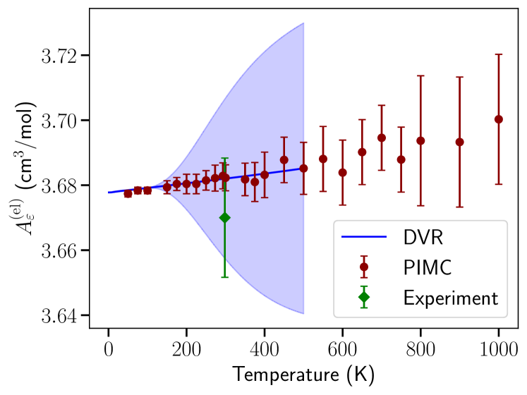
Figure 1: The electronic polarizability contribution to $A_{\varepsilon}$, $A_{\varepsilon}^{\mathrm{(el)}}$, of H${}_{2}{}^{16}$O as a function of temperature, obtained from computer simulations. The blue line is the result of our DVR calculations, together with an estimated uncertainty coming from the limited number of angular momenta that have been considered, reported as a blue area. Filled circles are the results of the path-integral simulations and the diamond is the experimental result of Ref. 5, adjusted to zero frequency using the dipole oscillator strength sums of Zeiss and Meath. [36] All uncertainties are reported at the $k=2$ coverage value and do not include the propagation of the unknown uncertainty of the water electronic polarizability surface.

Let us begin our discussion by considering the electronic polarizability contribution to the first virial coefficient, that is $\alpha_{\mathrm{el}}(T)$ defined in Eq. (9). As a first approximation, e.g., by using a classical rigid model for the water molecule, it can be calculated as the value of the electronic polarizability surface at the average geometric parameters (distances and angles) of the molecular ground state; [12] in this case one obtains the value $A_{\varepsilon}^{\mathrm{(el)}}=3.659$ cm³/mol. However, one should in fact average the value of the electronic polarizability surface over the distribution of configurations sampled by the ground state of the water molecule. This procedure, performed using the DVR ground-state wavefunction, provides $A_{\varepsilon}^{\mathrm{(el)}}=3.678$ cm³/mol and shows that a simple classical model underestimates the actual value by $-0.5\%$ in the $T\to 0$ limit. Comparing the ground-state averaged value of the electronic polarizability with its value at the geometry where the intramolecular potential has its minimum ($r_{1}=r_{2}=0.9579$ Å and $\theta=104.512^{\circ}$, corresponding to $A_{\varepsilon}^{\mathrm{(el,min)}}=3.566$ cm³/mol), one immediately obtains an estimate of the so-called vibrational contribution to the isotropic electronic polarizability, which is due to the zero-point (ZP) motion of the water molecule. In our case we obtain $\alpha_{\mathrm{el}}^{\mathrm{ZP}}=0.2986$ a.u., in very good agreement with analogous calculations in the literature. [37, 3]

The actual values for the electronic polarizability contribution to the first virial coefficient of water are reported in Table 1 and Fig. 1. We notice that our two calculation methods, PIMC and DVR, agree within mutual uncertainties at all the temperatures investigated in the present work. The PIMC approach is relatively noisy, but the DVR calculations clearly show that the electronic polarizability is a slightly increasing function of the temperature, exceeding its ground-state value by $\sim 0.04\%$ at $T=100$ K. Unfortunately, we are not aware of any characterization of the uncertainty associated with the electronic polarizability surface [3] and hence we cannot provide a precise quantitative assessment of the uncertainty of $A_{\varepsilon}^{\mathrm{(el)}}$.

Table 1: The values of the electronic polarizability contribution to $A_{\varepsilon}$ for H${}_{2}{}^{16}$O. All of the uncertainties are reported at $k=2$ coverage and do not include the propagation of the unknown uncertainty of the water electronic polarizability surface.

Temperature	$A_{\varepsilon}^{\mathrm{(el)}}$ (path-integral)	$A_{\varepsilon}^{\mathrm{(el)}}$ (DVR)
(K)	(cm3/mol)	(cm3/mol)
$1$	$–$	$3.67777\pm 0.00001$
$10$	$–$	$3.67786\pm 0.00007$
$25$	$–$	$3.67814\pm 0.00016$
$50$	$3.677\pm 0.001$	$3.67845\pm 0.00014$
$75$	$3.678\pm 0.001$	$3.67880\pm 0.00013$
$100$	$3.678\pm 0.001$	$3.67915\pm 0.00002$
$125$	$3.678\pm 0.001$	$3.6795\pm 0.0010$
$150$	$3.679\pm 0.002$	$3.680\pm 0.002$
$175$	$3.680\pm 0.002$	$3.680\pm 0.005$
$200$	$3.680\pm 0.003$	$3.681\pm 0.008$
$225$	$3.680\pm 0.003$	$3.681\pm 0.012$
$250$	$3.681\pm 0.003$	$3.681\pm 0.016$
$273.16$	$3.682\pm 0.004$	$3.68\pm 0.02$
$293.15$	$3.683\pm 0.004$	$3.68\pm 0.02$
$300$	$3.682\pm 0.004$	$3.68\pm 0.02$
$325$	$3.682\pm 0.004$	$3.68\pm 0.02$
$350$	$3.682\pm 0.005$	$3.68\pm 0.03$
$375$	$3.681\pm 0.006$	$3.68\pm 0.03$
$400$	$3.683\pm 0.007$	$3.68\pm 0.04$
$450$	$3.688\pm 0.007$	$3.68\pm 0.04$
$500$	$3.685\pm 0.007$	$3.69\pm 0.04$
$550$	$3.688\pm 0.008$	$–$
$600$	$3.68\pm 0.01$	$–$
$650$	$3.69\pm 0.01$	$–$
$700$	$3.69\pm 0.01$	$–$
$750$	$3.69\pm 0.01$	$–$
$800$	$3.69\pm 0.02$	$–$
$900$	$3.69\pm 0.02$	$–$
$1000$	$3.70\pm 0.02$	$–$
$1250$	$3.70\pm 0.03$	$–$
$1500$	$3.72\pm 0.04$	$–$
$1750$	$3.71\pm 0.04$	$–$
$2000$	$3.74\pm 0.06$	$–$

These results for $A_{\varepsilon}^{\mathrm{(el)}}$ can be compared to optical measurements of the refractivity of water vapor. The two most precise studies of this quantity were performed by Schödel et al. [4] and by Egan. [5] In order to compare with our static values of $A_{\varepsilon}^{\mathrm{(el)}}$, the results must be adjusted to zero frequency; this can be done with the dipole oscillator strength sums of Zeiss and Meath. [36] The resulting values (at 293.15 K in both cases) are approximately 3.67 cm³/mol, with expanded uncertainties on the order of 0.5%. This is in reasonable agreement with the values calculated here, although the comparison suggests that the polarizability surface of Lao et al. [3] may yield polarizabilities that are slightly too large (another possibility is inaccuracy in the dipole oscillator strengths of Ref. 36).

We also developed a correlation for $A_{\varepsilon}^{\mathrm{(el)}}$ by fitting the numerical data using a function of the form

$$A_{\varepsilon}^{\mathrm{(el)}}(T)=a+\frac{bT}{1+\exp\left[-(T-c)/T_{0}\right]}.$$ (33)

The values of the fitted parameters in Eq. (33) for the water isotopologues reported in this study are reported in Table 2. The correlation reproduces the values reported in Table 1 within the assigned uncertainties in the temperature range between 1 and 2000 K.

Table 2: Values of the parameters in Eq. (33) for the water isotopologues studied in this paper. The parameter $T_{0}$ has been set to $1$ K.

Isotopologue	$a$	$b/10^{-5}$	$c$
	(cm3/(mol K))	(cm3/(mol K))	(K)
H${}_{2}{}^{16}$O	$3.67777$	$1.38466$	$8.84684$
HD16O	$3.66227$	$1.3733$	$9.63151$
D${}_{2}{}^{16}$O	$3.6466$	$1.39401$	$5.3719$

VI.2 Dipolar polarizability

Table 3: The values of the dipolar contribution to $A_{\varepsilon}$ for H${}_{2}{}^{16}$O using various models, and its total value (last column) from path-integral simulations. All of the uncertainties are reported at $k=2$ coverage and do not include the propagation of the unknown uncertainty of the water dipole-moment surface and potential-energy surface. A breakdown of the rotational and vibrational contributions to $A_{\varepsilon}^{\mathrm{(dip)}}$ for H₂O is reported in Table I of the Supplementary Material.

Temperature	$A_{\varepsilon}^{\mathrm{(dip)}}$ (semiclassical)	$A_{\varepsilon}^{\mathrm{(dip)}}$ (HITRAN2020)	$A_{\varepsilon}^{\mathrm{(dip)}}$ (rigid)	$A_{\varepsilon}^{\mathrm{(dip)}}$ (flexible)	$A_{\varepsilon}$ (flexible)
(K)	(cm3/mol)	(cm3/mol)	(cm3/mol)	(cm3/mol)	(cm3/mol)
$50$	$349.494$	350 $\pm$ 12	356.2 $\pm$ 0.4	350 $\pm$ 6	353 $\pm$ 6
$75$	$248.944$	248 $\pm$ 9	251.18 $\pm$ 0.12	248 $\pm$ 2	252 $\pm$ 2
$100$	$192.688$	191 $\pm$ 7	193.62 $\pm$ 0.07	191.1 $\pm$ 1.3	194.8 $\pm$ 1.3
$125$	$157.021$	155 $\pm$ 5	157.54 $\pm$ 0.05	156.1 $\pm$ 1.0	159.7 $\pm$ 1.0
$150$	$132.445$	131 $\pm$ 5	132.75 $\pm$ 0.03	131.5 $\pm$ 0.7	135.2 $\pm$ 0.7
$175$	$114.501$	114 $\pm$ 4	114.70 $\pm$ 0.02	113.3 $\pm$ 0.6	117.0 $\pm$ 0.6
$200$	$100.829$	100 $\pm$ 4	100.985 $\pm$ 0.015	100.1 $\pm$ 0.6	103.8 $\pm$ 0.6
$225$	$90.069$	89 $\pm$ 3	90.173 $\pm$ 0.013	89.4 $\pm$ 0.6	93.1 $\pm$ 0.6
$250$	$81.381$	81 $\pm$ 3	81.482 $\pm$ 0.010	81.0 $\pm$ 0.6	84.7 $\pm$ 0.6
$273.16$	$74.704$	74 $\pm$ 3	74.779 $\pm$ 0.009	74.3 $\pm$ 0.6	78.0 $\pm$ 0.6
$293.15$	$69.763$	69 $\pm$ 2	69.833 $\pm$ 0.008	69.1 $\pm$ 0.6	72.8 $\pm$ 0.6
$300$	$68.216$	68 $\pm$ 2	68.290 $\pm$ 0.007	67.6 $\pm$ 0.6	71.3 $\pm$ 0.6
$325$	$63.110$	63 $\pm$ 2	63.162 $\pm$ 0.006	62.8 $\pm$ 0.6	66.5 $\pm$ 0.6
$350$	$58.715$	58 $\pm$ 2	58.761 $\pm$ 0.005	58.5 $\pm$ 0.6	62.2 $\pm$ 0.6
$375$	$54.892$	55 $\pm$ 2	54.931 $\pm$ 0.005	54.5 $\pm$ 0.6	58.2 $\pm$ 0.6
$400$	$51.536$	51 $\pm$ 2	51.575 $\pm$ 0.004	51.2 $\pm$ 0.6	54.9 $\pm$ 0.6
$450$	$45.920$	46 $\pm$ 2	45.951 $\pm$ 0.003	45.8 $\pm$ 0.5	49.5 $\pm$ 0.5
$500$	$41.408$	41.3 $\pm$ 1.4	41.431 $\pm$ 0.003	41.4 $\pm$ 0.7	45.1 $\pm$ 0.7
$550$	$37.703$	37.6 $\pm$ 1.3	37.726 $\pm$ 0.002	37.3 $\pm$ 0.6	41.0 $\pm$ 0.6
$600$	$34.606$	34.5 $\pm$ 1.2	34.6220 $\pm$ 0.0018	34.5 $\pm$ 0.7	38.2 $\pm$ 0.7
$650$	$31.980$	31.9 $\pm$ 1.1	31.9963 $\pm$ 0.0016	32.1 $\pm$ 0.8	35.8 $\pm$ 0.8
$700$	$29.724$	29.7 $\pm$ 1.0	29.7340 $\pm$ 0.0014	29.6 $\pm$ 0.7	33.3 $\pm$ 0.7
$750$	$27.765$	27.7 $\pm$ 1.0	27.7743 $\pm$ 0.0011	27.7 $\pm$ 0.6	31.4 $\pm$ 0.6
$800$	$26.048$	26.0 $\pm$ 0.9	26.0568 $\pm$ 0.0010	26.0 $\pm$ 0.7	29.7 $\pm$ 0.7
$900$	$23.182$	23.1 $\pm$ 0.8	23.1874 $\pm$ 0.0008	23.1 $\pm$ 0.7	26.9 $\pm$ 0.7
$1000$	$20.884$	20.8 $\pm$ 0.8	20.8891 $\pm$ 0.0006	20.6 $\pm$ 0.6	24.3 $\pm$ 0.6
$1250$	$16.736$	16.5 $\pm$ 0.7	16.7398 $\pm$ 0.0004	16.5 $\pm$ 0.7	20.2 $\pm$ 0.7
$1500$	$13.962$	13.5 $\pm$ 0.7	13.9650 $\pm$ 0.0003	13.9 $\pm$ 0.6	17.6 $\pm$ 0.6
$1750$	$11.977$	11.1 $\pm$ 0.6	11.9789 $\pm$ 0.0002	11.8 $\pm$ 0.5	15.6 $\pm$ 0.5
$2000$	$10.487$	9.2 $\pm$ 0.6	10.48780 $\pm$ 0.00016	10.4 $\pm$ 0.6	14.1 $\pm$ 0.6

In order to discuss the dipolar contribution to the first dielectric virial coefficient, which is reported in Table 3 for various water models, let us begin by considering a classical rigid model (cf. Eq. (7)). The most striking difference with respect to the electronic polarizability contribution is the explicit appearance of a dependence on the inverse of the temperature. As a consequence, the values of $A_{\varepsilon}^{\mathrm{(dip)}}$ cover a significantly larger range than those of $A_{\varepsilon}^{\mathrm{(el)}}$. Therefore, we will plot the product of $A_{\varepsilon}^{\mathrm{(dip)}}$ and the temperature $T$.

Using the same water geometry as before, [12] the dipole moment evaluated using the latest surface [3] would provide a value $\mu=1.860$ D ($1$ D $\approx 3.33564\times 10^{-30}$ C m); the square root of the average value of the dipole moment squared on the ground state of water is $\sqrt{\langle|\mathbf{m}|^{2}\rangle}=1.857$ D using the same model. However, the smallness of the moments of inertia of water makes quantum rotational effects sizable; these can be investigated either with the semiclassical correction of Eq. (8) or with the more accurate path-integral simulation for rigid rotors described in Sec. IV.2.1.

We report in Fig. 2 and Table 3 the values of the dipolar contribution to $A_{\varepsilon}$ for several water models. The semiclassical approach and quantum rigid approach are in very good agreement for temperatures $T\gtrsim 100$ K. Additionally, quantum rotational effects are already appreciable at room temperature, where they contribute to a reduction of the dielectric virial coefficient by $\sim 3\%$ with respect to a classical value. Quantum rotational effects become progressively more important at lower temperatures, resulting in a reduction of $\sim 10\%$ at $100$ K and $\sim 20\%$ at $50$ K. The results of rigid-model PIMC calculations are in perfect agreement with the results obtained by diagonalization of the Hamiltonian of Eq. (32).

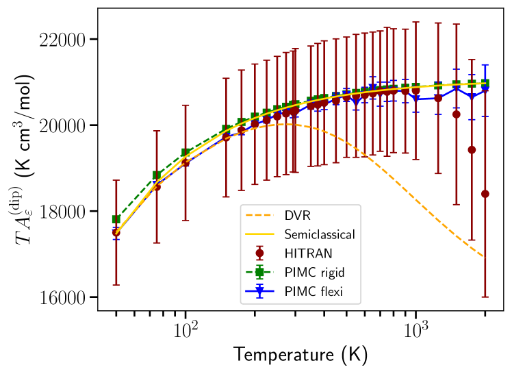
Figure 2: The dipolar contribution to $A_{\varepsilon}$, $A_{\varepsilon}^{\mathrm{(dip)}}$, multiplied by the temperature $T$ of H${}_{2}{}^{16}$O as a function of temperature. Red circles: values and uncertainties obtained from HITRAN2020 data. Green squares: values obtained using a rigid quantum mechanical model. Blue triangles: values obtained using a flexible quantum mechanical model solved using PIMC. Dashed orange line: values obtained using a flexible quantum mechanical model, solved using DVR (the discrepancies for $T>300$ K are due to insufficient convergence in the calculation of angular momentum states). Solid gold line: semiclassical values from Eq. (8). All theoretical uncertainties are reported at the $k=2$ coverage value and do not include the propagation of the unknown uncertainty of the water dipole-moment surface. The lines joining the symbols are a guide to the eye.

Figure 2 also shows the effect of molecular flexibility in determining $A_{\varepsilon}^{\mathrm{(dip)}}$, as well as presenting the experimental values derived from the HITRAN2020 database. In general, the addition of flexibility results in a reduction of the dipolar contribution to the first dielectric virial coefficient, which is particularly evident at $T\leq 150$ K. The path-integral calculations are in very good agreement with values derived from spectroscopy, falling well within the estimated experimental uncertainty. We emphasize that we are not aware of any uncertainty estimates for the electronic-polarizability or dipole-moment surfaces, so we cannot provide a rigorous uncertainty analysis on $A_{\varepsilon}$ at present and only its statistical contribution is reported. For the sake of a meaningful comparison, we collected enough statistics in the Monte Carlo calculations to make the statistical uncertainty smaller than the experimental one. The average values of our simulations and those computed from HITRAN2020 are in very good agreement at all the temperatures studied.

The computed and experimental values of $A_{\varepsilon}^{\mathrm{(dip)}}$ begin to differ at high temperature; this is evident for $T\geq 1500$ K in the case of H${}_{2}{}^{16}$O and at even smaller temperatures for other isotopologues (as shown in Figures 2 and 5 of the Supplementary Material). We think that this discrepancy is due to the limited coverage of high-energy rovibrational states in the HITRAN2020 database, which limits the accuracy of the deduced values of $A_{\varepsilon}^{\mathrm{(dip)}}$ at high temperatures.

Figure 2 also reports the calculation of $A_{\varepsilon}^{\mathrm{(dip)}}$ performed using the DVR approach. The agreement with the path-integral calculation and with HITRAN2020 data is very good at temperatures $T\lesssim 300$ K. For higher temperatures, the DVR approach suffers from the limited number of angular momentum states $J$ that we have been able to compute, and therefore the DVR values diverge from those obtained using PIMC.

The last column of Table 3 reports our theoretical estimate for the first dielectric virial coefficient of water, which has been obtained by summing the value of the dipolar contribution obtained using a flexible model of water (next-to-last column of the same table) and the electronic contribution reported in Table 1.

Finally, we have also fitted the values of $A_{\varepsilon}^{\mathrm{(dip)}}(T)$ computed using PIMC to a correlation of the form

$$A_{\varepsilon}^{\mathrm{(dip)}}(T)=\frac{a(1+d/T)/T}{1+\exp\left[-(T-b)/c\right]}.$$ (34)

Values of the parameters $a$, $b$, $c$, and $d$ in Eq. (34) are reported in Table 4.

Table 4: Values of the parameters in Eqs. (34) and (37) for the water isotopologues studied in this paper.

Isotopologue	$a$	$b$	$c$	$d$
	(K cm3/mol)	(K)	(K)	(K2 cm3/mol)
H${}_{2}{}^{16}$O	$20945.9$	$-693.079$	$184.074$	$-7.46202$
HD16O	$21950.5$	$-11979.3$	$4072.31$	$-6.30806$
D${}_{2}{}^{16}$O	$23949.4$	$-17378.8$	$9154.42$	$-4.5188$

VI.3 Vibrational polarizability

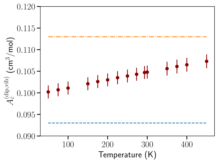
Figure 3: The vibrational polarizability contribution to $A_{\varepsilon}$, $A^{\textrm{(dip,vib)}}_{\varepsilon}$, of H${}_{2}{}^{16}$O as a function of temperature, computed from spectroscopic information in the HITRAN2020 database. [16] The blue dashed line is the value 0.093 cm³/mol calculated from a more crude use of spectroscopic data by Bishop and Cheung.[38] The orange dot-dashed line is the value 0.113 cm³/mol from the ab initio calculations of Ruud et al.[39]

Because the HITRAN2020 database allows us to distinguish between vibrational transitions and those in which only the rotational quantum numbers change, we can separate the calculated $A_{\varepsilon}^{\mathrm{(dip)}}$ into vibrational and rotational parts. The detailed results for H${}_{2}{}^{16}$O, HD¹⁶O, and D${}_{2}{}^{16}$O are given in the Supplementary Material. The rotational contribution $\left(A^{\mathrm{(dip,rot)}}_{\varepsilon}\right)$ is larger than the vibrational contribution $\left(A^{\mathrm{(dip,vib)}}_{\varepsilon}\right)$ by roughly a factor of 600 at 300 K; our computed $A^{\mathrm{(dip,vib)}}_{\varepsilon}$ have a small temperature dependence and for H${}_{2}{}^{16}$O have values slightly above 0.10 cm³/mol at typical temperatures of experimental interest (see Fig. 3).

The vibrational contribution to $A_{\varepsilon}^{\mathrm{(dip)}}$ can be related to the molecule’s vibrational polarizability, $\alpha_{\mathrm{vib}}$, by

$$A^{\mathrm{(dip,vib)}}_{\varepsilon}=\frac{4\pi}{3}N_{\mathrm{A}}\alpha_{\mathrm{vib}}.$$ (35)

Our calculations produce $\alpha_{\mathrm{vib}}$ whose magnitude is roughly 3% of the magnitude of the electronic polarizability; this is often considered an additional contribution when compiling the static polarizabilities of molecules.[40]

The vibrational polarizability has been a subject of some study, allowing comparison to previous estimates. Bishop and Cheung[38] estimated $\alpha_{\mathrm{vib}}$ for H₂O and HDO based on the positions and integrated intensities of the three primary vibrational bands of the ground state. This can be thought of as an approximation to Eq. (25) in which each vibrational band is lumped into one line. Ruud et al.[39] estimated $\alpha_{\mathrm{vib}}$ from ab initio calculations of a perturbation expansion of each normal vibration. The values of $A^{\mathrm{(dip,vib)}}_{\varepsilon}$ derived from Refs. 38 and 39 for H₂O are 0.093 cm³/mol and 0.113 cm³/mol, respectively. These literature estimates are in reasonable agreement with our results, as shown in Fig. 3.

Bishop and Cheung made a similar estimate for the HDO molecule, producing $A^{\mathrm{(dip,vib)}}_{\varepsilon}$ = 0.107 cm³/mol, which underestimates the vibrational polarizability (see Table IV in the Supplementary Material) by an amount somewhat less than that shown in Fig. 3 for H₂O.

VI.4 Dipole moment

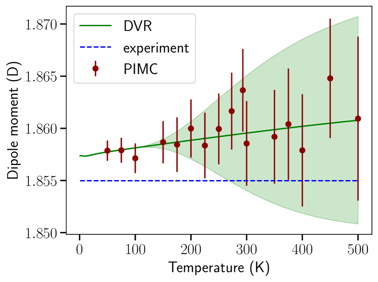
Figure 4: The average dipole moment of H${}_{2}{}^{16}$O from our DVR (solid line) and PIMC (points) calculations. The shaded area denotes an estimate of the uncertainty of the DVR calculation. The PIMC error bars represent the expanded $(k=2)$ statistical uncertainty of the Monte Carlo calculation. The dashed line reports the experimental ground-state value of $1.85498$ D from Ref. 6.

We also computed the temperature-dependent value of the average dipole moment, defined as

$$\mu(T)=\sqrt{\sum_{J\nu}\frac{g_{J\nu}(2J+1)\mathrm{e}^{-\beta E_{J\nu}}}{Q_{1}(\beta,0)}\langle\psi_{J\nu}||\mathbf{m}|^{2}|\psi_{J\nu}\rangle},$$ (36)

where, as above, $J$ and $\nu$ are the total angular momentum of the water molecule, $\nu$ are vibrational quantum numbers and $g_{J\nu}$ is the degeneracy of these states. The results are reported in Fig. 4, where we also plot the experimental ground-state value of $\mu$. [6] Similarly to what has been observed above, the PIMC calculations are rather noisy, but agree with the DVR results up to the highest temperature that we have investigated. We also report an estimate of the uncertainty of our DVR calculations, which is mainly due to the finite number of angular momentum states $J$ considered in this work. A slight increase of the dipole moment with temperature is apparent in both cases (on the order of $0.2\%$ from $0$ K to $500$ K), although the trend is probably clearer from the DVR results.

The value of the dipole moment at 0 K is that in the ground rovibrational state. The DVR calculations yield a dipole moment of 1.8574 D for H₂¹⁶O, which is about 0.13% larger than the highly accurate ground-state value of 1.85498(9) D measured by Shostak et al. [6] A similar calculation for D${}_{2}{}^{16}$O yields a ground-state dipole moment of 1.8565 D, which exceeds by approximately 0.11% the experimental value of 1.8545(4) D measured by Dyke and Muenter. [41] These two comparisons with high-accuracy experimental results suggest that the dipole-moment surface we used, [20] which was designed more for spectroscopic applications than for accurate values of the dipole moment itself, is slightly biased toward high values.

VI.5 Rescaled dipolar polarizability

The slightly too large dipole moments discussed in the previous section will result in a slightly overestimated dipolar polarizability. This can, however, be simply corrected for because all contributions to the dipolar polarizability are proportional to the square of the dipole moment. We can therefore produce an improved estimate of the dipolar polarizability by multiplying Eq. (34) by the square of the ratio of the true ground-state dipole moment to that obtained here; for that purpose we use the H₂O value since it is the most accurately measured, producing a factor of $(1.85498/1.8574)^{2}\approx 0.9974$. The rescaled dipolar polarizability is therefore given by

$$A_{\varepsilon}^{\mathrm{(dip,r)}}(T)=0.9974\frac{a(1+d/T)/T}{1+\exp\left[-(T-b)/c\right]},$$ (37)

with the parameters given in Table 4. At all temperatures, the magnitude of this correction is smaller than the standard statistical uncertainty of the calculation of $A_{\varepsilon}^{\mathrm{(dip)}}$.

Table 5: The values of the average dipole moment $\mu(T)$ of H${}_{2}{}^{16}$O (Debye) from Eq. (36) The PIMC uncertainties represent the expanded $(k=2)$ statistical uncertainty of the Monte Carlo calculation. Uncertainties do not include the propagation of the unknown uncertainty of the water dipole-moment surface.

Temperature	$\mu(T)$ (PIMC)	$\mu(T)$ (DVR)
(K)	(D)	(D)
$1$	$–$	$1.85737\pm 0.00001$
$10$	$–$	$1.85734\pm 0.00002$
$25$	$–$	$1.85749\pm 0.00004$
$50$	$1.858\pm 0.001$	$1.85774\pm 0.00003$
$75$	$1.858\pm 0.001$	$1.85794\pm 0.00003$
$100$	$1.857\pm 0.001$	$1.85813\pm 0.00010$
$125$	$1.859\pm 0.001$	$1.8583\pm 0.0003$
$150$	$1.859\pm 0.002$	$1.8585\pm 0.0005$
$175$	$1.858\pm 0.003$	$1.8587\pm 0.0010$
$200$	$1.860\pm 0.003$	$1.859\pm 0.002$
$225$	$1.858\pm 0.003$	$1.859\pm 0.003$
$250$	$1.860\pm 0.003$	$1.859\pm 0.004$
$273.16$	$1.862\pm 0.004$	$1.859\pm 0.005$
$293.15$	$1.864\pm 0.004$	$1.860\pm 0.005$
$300$	$1.859\pm 0.004$	$1.860\pm 0.006$
$325$	$1.860\pm 0.004$	$1.860\pm 0.006$
$350$	$1.859\pm 0.004$	$1.860\pm 0.007$
$375$	$1.860\pm 0.005$	$1.860\pm 0.008$
$400$	$1.858\pm 0.005$	$1.860\pm 0.008$
$450$	$1.865\pm 0.006$	$1.860\pm 0.009$
$500$	$1.861\pm 0.008$	$1.861\pm 0.010$
$600$	$1.858\pm 0.009$	$–$
$650$	$1.855\pm 0.009$	$–$
$700$	$1.873\pm 0.011$	$–$
$750$	$1.861\pm 0.012$	$–$
$800$	$1.858\pm 0.013$	$–$
$900$	$1.864\pm 0.013$	$–$
$1000$	$1.868\pm 0.014$	$–$
$1250$	$1.863\pm 0.017$	$–$
$1500$	$1.870\pm 0.020$	$–$
$1750$	$1.868\pm 0.021$	$–$
$2000$	$1.870\pm 0.025$	$–$

VII Conclusions

This work has presented the first complete theoretical calculation of water’s first dielectric virial coefficient, $A_{\varepsilon}$, taking into account the flexibility of the water molecule and state-of-the-art descriptions of the variation of the electronic polarizability and the dipole moment with molecular geometry. The path-integral method, and in some cases the DVR approach to the three-body Hamiltonian, are used to perform the calculations with full accounting for quantum effects.

The contribution of the electronic polarizability to $A_{\varepsilon}$ is not constant as is typically assumed, but increases slightly with temperature due to the different polarizabilities of states other than the rovibrational ground state. Our results are consistent with the best experimental values for this quantity, which are obtained from measurements of the refractive index.[4, 5]

The contribution of the dipolar polarizability also differs somewhat from the classical $\frac{\mu^{2}}{3k_{\mathrm{B}}T}$ functional form, both because values of the dipole moment other than the ground-state value are sampled at finite temperature and because of the quantization of rotation. The latter effect reduces the dipolar contribution to $A_{\varepsilon}$ by roughly 3% at room temperature. The calculated dipolar contribution to $A_{\varepsilon}$ also agrees well with estimates using line positions and intensities in the HITRAN2020 database.

In addition to the dominant isotopologue H₂¹⁶O, we performed calculations for D₂¹⁶O and HD¹⁶O. The data are presented in the Supplementary Material, but we note here that there is nothing surprising in the results. The electronic polarizability (and therefore $A_{\varepsilon}^{\mathrm{(el)}}$) is smaller by amounts on the order of 0.5% for HD¹⁶O and 1% for D₂¹⁶O. This probably reflects the shorter average length of O–D bonds compared to O–H bonds. The dipole moment is slightly reduced by D substitution, in agreement with the experimental result for D₂¹⁶O. [41] The dipolar contribution $A_{\varepsilon}^{\mathrm{(dip)}}$ is not affected (within the uncertainty of our calculations) by D substitution at high temperatures. However, below about 500 K, D substitution noticeably increases $A_{\varepsilon}^{\mathrm{(dip)}}$. This is because the substitution increases the moment of inertia, reducing the magnitude of the (negative) correction to $A_{\varepsilon}^{\mathrm{(dip)}}$ due to the quantization of rotation [expressed semiclassically by Eq. (8)].

Our results for $A_{\varepsilon}$ provide accurate, temperature-dependent data that can be used to describe the effect of water on the static dielectric constant of gases for humidity metrology. They can also serve as a low-density boundary condition for future comprehensive formulations for the static dielectric constant of H₂O and D₂O. We note that the current international standard formulation for the dielectric constant of H₂O[42, 43] does not account for the quantum effects studied in this work; it also uses a dipole moment that is roughly 1% smaller than the best experimental value, [6] which in our terminology produces a value of $A_{\varepsilon}^{\mathrm{(dip)}}$ that is roughly 2% too small. Our results for $A_{\varepsilon}^{\mathrm{(el)}}$ could also be used to improve the standard formulation for the refractive index of water, [43, 44] although this would require a dispersion correction from our static values to optical frequencies.

Our recommended formula for $A_{\varepsilon}(T)$ is given by

$$A_{\varepsilon}(T)=A_{\varepsilon}^{\mathrm{(el)}}(T)+A^{\mathrm{(dip,r)}}_{\varepsilon}(T),$$ (38)

where the electronic polarizability contribution $A_{\varepsilon}^{\mathrm{(el)}}$ is given by Eq. (33) and the (rescaled) dipolar contribution $A^{\textrm{(dip,r)}}_{\varepsilon}$ is given by Eq. (37).

Extension beyond the low-density limit would require the second dielectric virial coefficient, $B_{\varepsilon}$. $B_{\varepsilon}$ can be computed in a straightforward way for noble gases,[10] but the calculation is much more difficult for a molecule like water. The largest effect would likely come from the correlation of molecular dipoles due to the pair potential; this would be relatively straightforward for a rigid, nonpolarizable model and Yang et al.[45] performed such a calculation for a simple water model. A complete calculation of $B_{\varepsilon}$ would require a multidimensional surface for the nonadditive electronic polarizability and for changes in multipole moments as the molecules mutually polarize each other. Incorporating the flexibility of the molecules would greatly increase the complexity, and is likely impractical at present. A classical calculation of $B_{\varepsilon}$ with a rigid, polarizable water model was performed by Stone et al.;[46] thus far the result has not been confirmed by independent calculations and unfortunately there seem to be no reliable experimental determinations of $B_{\varepsilon}$. Additional rigorous calculations of $B_{\varepsilon}$ for water would therefore be desirable.

VIII Supplementary Material

The Supplementary Material includes the following: derivation of Eqs. (9) and (10), a table with the breakdown of the vibrational and rotational contributions to $A_{\varepsilon}^{\mathrm{(dip)}}$ for H₂O. Tables and figures reporting $A_{\varepsilon}^{\mathrm{(el)}}$ and dipole moments of HDO and D₂O. Tables and figures reporting the computed $A_{\varepsilon}^{\mathrm{(dip)}}$ for HDO and D₂O, their division into vibrational and rotational contributions, and their derivation from HITRAN2020 data

IX Acknowledgments

We thank Joseph T. Hodges of NIST for helpful discussions about HITRAN and spectroscopic data, Patrick Egan of NIST for discussions on water’s refractivity, and the University of Trento for a generous allocation of computing resources on their HPC Cluster.

Author Declarations

Conflict of Interest

The authors have no conflicts to disclose.

Data Availability

The data that support the findings of this study are available within the article and its Supplementary Material.

Appendix A Wavefunction expression for $\alpha_{\mathrm{dip}}(T)$

A.1 Flexible models

The derivation of the expression of $\alpha_{\mathrm{dip}}(T)$ starts from the general formula of Eq. (10) and the representation of the molecular quantum states of Eq. (19). In fact, the indices $i$ and $j$ in Eq. (10) stand for all the quantum numbers needed to describe a given molecular state, that is $i\equiv J\nu mI$. Correspondingly, we will indicate the quantum numbers corresponding to the index $j$ with primed quantities, i.e., $j\equiv J^{\prime}\nu^{\prime}m^{\prime}I^{\prime}$. Since energies depend only on the quantum numbers $J$ and $\nu$, and since the matrix element of the dipole moment operator does not act on the nuclear spins, one can perform the sum over $I$ and $I^{\prime}$ obtaining

$$\sum_{I,I^{\prime}}\left|\chi^{*}({\cal I}_{J\nu},I)\chi({\cal I}_{J^{\prime}\nu^{\prime}},I^{\prime})\right|^{2}=g_{J\nu}\delta_{g_{J\nu},g_{J^{\prime}\nu^{\prime}}},$$ (39)

that is, the sum over the nuclear spin states allows only ortho-ortho or para-para transitions, and provides the corresponding degeneracy factor.

Additionally, particular care must be taken to evaluate the matrix element of $\mathbf{m}\cdot\mathbf{e}$, where we will assume, without loss of generality, that we are considering $\mathbf{e}$ aligned along the $Z$ axis in the laboratory frame. However, the DVR procedure writes the wavefunction with coordinates $q$ that are defined in the so-called molecular frame, where the orientation of the molecule is fixed. In order to evaluate the matrix elements of $\mathbf{m}_{Z}$, one has to recall that it transforms as the $0$-th component of a vector operator, which means that it is given by [28, 11, 25]

$$\mathbf{m}_{0}^{\mathrm{L}}=\sum_{K=1}^{1}\mathbf{m}_{K}^{\mathrm{M}}(q)D^{1*}_{0K}(\Omega),$$ (40)

where the superscript ‘L’ denotes the spherical components of the operator in the laboratory-fixed frame, and the superscript ‘M’ denotes spherical components in the molecule-fixed frame. Using the identities

$$\int D^{J_{1}}_{m_{1}k_{1}}(\Omega)D^{J_{2}}_{m_{2}k_{2}}(\Omega)D^{J_{3}}_{m_{3}k_{3}}(\Omega)\mathrm{d}\Omega =$$

$$8\pi^{2}\left(\begin{array}[]{ccc}J_{1}&J_{2}&J_{3}\\ m_{1}&m_{2}&m_{3}\end{array}\right)\left(\begin{array}[]{ccc}J_{1}&J_{2}&J_{3}\\ k_{1}&k_{2}&k_{3}\end{array}\right)$$ (45)

$$\sum_{mm^{\prime}}\left(\begin{array}[]{ccc}J^{\prime}&1&J\\ m^{\prime}&0&m\end{array}\right) = \frac{1}{3}$$ (48)

one arrives from Eq. (10) to

$$\alpha_{\mathrm{dip}}(T)=\sum_{J^{\prime}\nu^{\prime},J\nu}\frac{(2J^{\prime}+1)(2J+1)}{3}\left|\sum_{k^{\prime}=k-1,k}^{k+1,\infty}\left\langle\psi_{J^{\prime}\nu^{\prime}k^{\prime}}|\mathbf{m}^{\mathrm{M}}_{k^{\prime}-k}|\psi_{J\nu k}\right\rangle(-1)^{k^{\prime}}\left(\begin{array}[]{ccc}J^{\prime}&1&J\\ -k^{\prime}&k^{\prime}-k&k\end{array}\right)\right|^{2}g_{J\nu}\delta_{g_{J\nu},g_{J^{\prime}\nu^{\prime}}}\frac{\mathrm{e}^{-\beta E_{J^{\prime}\nu^{\prime}}}-\mathrm{e}^{-\beta E_{J\nu}}}{E_{J\nu}-E_{J^{\prime}\nu^{\prime}}},$$ (49)

where, in the DVR approach, one has

$$\left\langle\psi_{J^{\prime}\nu^{\prime}k^{\prime}}|\mathbf{m}^{\mathrm{M}}_{k^{\prime}-k}|\psi_{J\nu k}\right\rangle=\sum_{q}\psi_{J^{\prime}\nu^{\prime}k^{\prime}}(q)\mathbf{m}^{\mathrm{M}}_{k^{\prime}-k}(q)\psi_{J\nu k}(q)$$ (50)

since the spherical components of the dipole-moment operator are diagonal in the molecule-fixed frame. In Eq. (49), the quantity $\left(\begin{array}[]{ccc}J^{\prime}&1&J\\ -k^{\prime}&k^{\prime}-k&k\end{array}\right)$ is a Wigner $3j$-symbol. The diagonalization procedure outlined in Sec. IV.1 provides, for any given angular momentum $J$, the energies $E_{J\nu}$ and the wavefunctions $\psi_{J\nu k}(q)$ (as the eigenvalues and eigenvectors of the three-body Hamiltonian in the molecule-fixed frame, respectively), enabling a straightforward evaluation of the dipolar polarizability using Eqs. (50) and (49). In this paper, we obtained the degeneracy factors $g_{J\nu}$ from the HITRAN2020 database.

A.2 Rigid models

Equation (49) is valid also in the case of rigid molecular models of water. In this case, the eigenfunctions do not depend on the coordinates $q$ describing the molecular vibrations, so that the matrix element of Eq. (50) is replaced by

$$\left\langle\psi_{J^{\prime}\nu^{\prime}k^{\prime}}|\mathbf{m}^{\mathrm{M}}_{k^{\prime}-k}|\psi_{J\nu k}\right\rangle=\psi_{J^{\prime}\nu^{\prime}k^{\prime}}\mathbf{m}^{\mathrm{M}}_{k^{\prime}-k}\psi_{J\nu k}$$ (51)

where now $\psi_{J\nu k}$ are the eigenfunctions of the rigid-rotor Hamiltonian (see Sec. V.1.2). In the case of a rigid molecule, the matrix elements of the spherical components of the dipole-moment operator, $\mathbf{m}^{\mathrm{M}}_{k^{\prime}-k}$, are constants.

References

- Cuccaro et al. [2012] R. Cuccaro, R. M. Gavioso, G. Benedetto, D. Madonna Ripa, V. Fernicola, and C. Guianvarc’h, “Microwave determination of water mole fraction in humid gas mixtures,” Int. J. Thermophys. 33, 1352 (2012).
- Gavioso et al. [2014] R. M. Gavioso, D. Madonna Ripa, R. Benyon, J. G. Gallegos, F. Perez-Sanz, S. Corbellini, S. Avila, and A. M. Benito, “Measuring humidity in methane and natural gas with a microwave technique,” Int. J. Thermophys. 35, 748 (2014).
- Lao et al. [2018] K. U. Lao, J. Jia, R. Maitra, and R. A. DiStasio, “On the geometric dependence of the molecular dipole polarizability in water: A benchmark study of higher-order electron correlation, basis set incompleteness error, core electron effects, and zero-point vibrational contributions,” J. Chem. Phys. 149, 204303 (2018).
- Schödel, Walkov, and Abou-Zeid [2006] R. Schödel, A. Walkov, and A. Abou-Zeid, “High-accuracy determination of water vapor refractivity by length interferometry,” Opt. Lett. 31, 1979 (2006).
- Egan [2022] P. F. Egan, “Capability of commercial trackers as compensators for the absolute refractive index of air,” Precision Eng. 77, 46 (2022).
- Shostak, Ebenstein, and Muenter [1991] S. L. Shostak, W. L. Ebenstein, and J. S. Muenter, “The dipole moment of water. I. Dipole moments and hyperfine properties of H2O and HDO in the ground and excited vibrational states,” J. Chem. Phys. 94, 5875 (1991).
- MacRury and Steele [1974] T. B. MacRury and W. A. Steele, “Quantum effects on the dielectric virial coefficients of polar gases,” J. Chem. Phys. 61, 3352 (1974).
- Gray, Gubbins, and Joslin [2011] C. G. Gray, K. E. Gubbins, and C. G. Joslin, Theory of Molecular Fluids, Vol. 2: Applications (Oxford Science Publications, 2011).
- Hill [1958] T. L. Hill, “Theory of the dielectric constant of imperfect gases and dilute solutions,” J. Chem. Phys. 28, 61 (1958).
- Garberoglio, Harvey, and Jeziorski [2021] G. Garberoglio, A. H. Harvey, and B. Jeziorski, “Path-integral calculation of the third dielectric virial coefficient of noble gases,” J. Chem. Phys. 155, 234103 (2021).
- Zare [1988] R. N. Zare, Angular Momentum: Understanding Spatial Aspects in Chemistry and Physics (Wiley, New York, 1988).
- Czakó, Mátyus, and Császár [2009] G. Czakó, E. Mátyus, and A. G. Császár, “Bridging theory with experiment: A benchmark study of thermally averaged structural and effective spectroscopic parameters of the water molecule,” J. Phys. Chem. A 113, 11665 (2009).
- Illinger and Smyth [1960] K. H. Illinger and C. P. Smyth, “Atomic polarization. I. Vibrational polarization of gases,” J. Chem. Phys. 32, 787 (1960).
- Bishop [1990] D. M. Bishop, “Molecular vibrational and rotational motion in static and dynamic electric fields,” Rev. Mod. Phys. 62, 343 (1990).
- Hilborn [1982] R. C. Hilborn, “Einstein coefficients, cross sections, -values, dipole moments, and all that,” Am. J. Phys. 50, 982 (1982).
- Gordon et al. [2021] I. E. Gordon et al., “The HITRAN2020 molecular spectroscopic database,” J. Quant. Spectrosc. Radiat. Trans. 277, 107949 (2021).
- Gamache and Rothman [1992] R. R. Gamache and L. S. Rothman, “Extension of the HITRAN database to non-LTE applications,” J. Quant. Spectrosc. Radiat. Trans. 48, 519 (1992).
- Šimečková et al. [2006] M. Šimečková, D. Jacquemart, L. S. Rothman, R. R. Gamache, and A. Goldman, “Einstein A-coefficients and statistical weights for molecular absorption transitions in the HITRAN database,” J. Quant. Spectrosc. Radiat. Trans. 98, 130 (2006).
- Mizus et al. [2018] I. I. Mizus, A. A. Kyuberis, N. F. Zobov, V. Y. Makhnev, O. L. Polyansky, and J. Tennyson, “High-accuracy water potential energy surface for the calculation of infrared spectra,” Phil. Trans. Royal Soc. A 376, 20170149 (2018).
- Conway et al. [2018] E. K. Conway, A. A. Kyuberis, O. L. Polyansky, J. Tennyson, and N. F. Zobov, “A highly accurate ab initio dipole moment surface for the ground electronic state of water vapour for spectra extending into the ultraviolet,” J. Chem. Phys. 149, 084307 (2018).
- Sutcliffe and Tennyson [1987] B. T. Sutcliffe and J. Tennyson, “Variational methods for the calculation of rovibrational energy levels of small molecules,” J. Chem. Soc., Faraday Trans. 2 83, 1663 (1987).
- Light and Carrington Jr [2000] J. C. Light and T. Carrington Jr, “Discrete-variable representations and their utilization,” Adv. Chem. Phys. 114, 263 (2000).
- Szalay [1993] V. Szalay, “Discrete variable representations of differential operators,” J. Chem. Phys. 99, 1978 (1993).
- Baye [2015] D. Baye, “The Lagrange-mesh method,” Phys. Rep. 565, 1 (2015).
- Tennyson et al. [2004] J. Tennyson, M. A. Kostin, P. Barletta, G. J. Harris, O. L. Polyansky, J. Ramanlal, and N. F. Zobov, “DVR3D: a program suite for the calculation of rotation–vibration spectra of triatomic molecules,” Comput. Phys. Commun. 163, 85 (2004).
- Czakó et al. [2004] G. Czakó, T. Furtenbacher, A. G. Császár, and V. Szalay, “Variational vibrational calculations using high-order anharmonic force fields,” Mol. Phys. 102, 2411 (2004).
- Mátyus et al. [2010] E. Mátyus, C. Fábri, T. Szidarovszky, G. Czakó, W. D. Allen, and A. G. Császár, “Assigning quantum labels to variationally computed rotational-vibrational eigenstates of polyatomic molecules,” J. Chem. Phys. 133, 034113 (2010).
- Le Sueur et al. [1992] C. R. Le Sueur, S. Miller, J. Tennyson, and B. T. Sutcliffe, “On the use of variational wavefunctions in calculating vibrational band intensities,” Mol. Phys. 76, 1147 (1992).
- Feynman and Hibbs [1965] R. P. Feynman and A. Hibbs, Quantum Mechanics and Path Integrals (McGraw-Hill, New York, 1965).
- Noya et al. [2011] E. G. Noya, L. M. Sesé, R. Ramírez, C. McBride, M. M. Conde, and C. Vega, “Path integral Monte Carlo simulations for rigid rotors and their application to water,” Mol. Phys. 109, 149 (2011).
- Noya, Vega, and McBride [2011] E. G. Noya, C. Vega, and C. McBride, “A quantum propagator for path-integral simulations of rigid molecules,” J. Chem. Phys. 134, 054117 (2011).
- Garberoglio et al. [2018] G. Garberoglio, P. Jankowski, K. Szalewicz, and A. H. Harvey, “Fully quantum calculation of the second and third virial coefficients of water and its isotopologues from ab initio potentials,” Faraday Discuss. 148, 174501 (2018).
- Bishop, Pipin, and Silverman [1986] D. M. Bishop, J. Pipin, and J. N. Silverman, “Methods for introducing vibrational effects in the calculation of electric dipole polarizabilities and hyperpolarizabilities (with reference to H),” Mol. Phys. 59, 165 (1986).
- Hellmann and Harvey [2020] R. Hellmann and A. H. Harvey, “First-principles diffusivity ratios for kinetic isotope fractionation of water in air,” Geophys. Res. Lett. 47, e2020GL089999 (2020).
- Tuckerman et al. [1993] M. E. Tuckerman, B. J. Berne, G. J. Martyna, and M. L. Klein, “Efficient molecular dynamics and hybrid Monte Carlo algorithms for path integrals,” J. Chem. Phys. 99, 2796 (1993).
- Zeiss and Meath [1977] G. D. Zeiss and W. J. Meath, “Dispersion energy constants , dipole oscillator strength sums and refractivities for Li, N, O, H2, N2, O2, NH3, H2O, NO and N2O,” Mol. Phys. 33, 1155 (1977).
- Avila [2005] G. Avila, “Ab initio dipole polarizability surfaces of water molecule: Static and dynamic at 514.5 nm,” J. Chem. Phys. 122, 144310 (2005).
- Bishop and Cheung [1982] D. M. Bishop and L. M. Cheung, “Vibrational contributions to molecular dipole polarizabilities,” J. Phys. Chem. Ref. Data 11, 119–133 (1982).
- Ruud, Jonsson, and Taylor [2000] K. Ruud, D. Jonsson, and P. R. Taylor, “Vibrational effects on electric and magnetic susceptibilities: application to the properties of the water molecule,” Phys. Chem. Chem. Phys. 2, 2161–2171 (2000).
- Hohm [2013] U. Hohm, “Experimental static dipole–dipole polarizabilities of molecules,” J. Mol. Struct. 1054-1055, 282–292 (2013).
- Dyke and Muenter [1973] T. R. Dyke and J. S. Muenter, “Electric dipole moments of low states of H2O and D2O,” J. Chem. Phys. 59, 3125 (1973).
- Fernández et al. [1997] D. P. Fernández, A. R. H. Goodwin, E. W. Lemmon, J. M. H. Levelt Sengers, and R. C. Williams, “A formulation for the static permittivity of water and steam at temperatures from 238 K to 873 K at pressures up to 1200 MPa, including derivatives and Debye–Hückel coefficients,” J. Phys. Chem. Ref. Data 26, 1125 (1997).
- Harvey, Hrubý, and Meier [2023] A. H. Harvey, J. Hrubý, and K. Meier, “Improved and Always Improving: Reference Formulations for Thermophysical Properties of Water,” J. Phys. Chem. Ref. Data 52, 011501 (2023).
- Harvey, Gallagher, and Levelt Sengers [1998] A. H. Harvey, J. S. Gallagher, and J. M. H. Levelt Sengers, “Revised Formulation for the Refractive Index of Water and Steam as a Function of Wavelength, Temperature and Density,” J. Phys. Chem. Ref. Data 27, 761 (1998).
- Yang, Schultz, and Kofke [2017] S. Yang, A. J. Schultz, and D. A. Kofke, “Evaluation of second and third dielectric virial coefficients for non-polarisable molecular models,” Mol. Phys. 115, 991 (2017).
- Stone, Tantirungrotechai, and Buckingham [2000] A. J. Stone, Y. Tantirungrotechai, and A. D. Buckingham, “The dielectric virial coefficient and model intermolecular potentials,” Phys. Chem. Chem. Phys. 2, 429 (2000).