Boltzmann’s Billiard Systems: Computation of the Billiard Mapping and Some Numerical Results

Abstract

L. Boltzmann proposed in [1] a billiard model with a planar central force problem reflected against a line not passing through the center. He asserted that such a system is ergodic, which thus illustrates his ergodic hypothesis. However, it has been recently shown that when the underlying central force problem is the Kepler problem, then the system is actually integrable [7]. This raises the question of whether Boltzmann’s assertion holds true for some central force problems that he considered. In this paper, we present some geometrical and numerical analysis on the dynamics of several of these systems. As indicated by the numerics, many of these systems show chaotic dynamics and a system seems to be ergodic.

1 Introduction

In [1], Boltzmann examined a billiard model in a potential field, which is defined with the central force problem in $\mathbb{R}^{2}$ with the potential

$$V_{\alpha,\beta}:=-\dfrac{\alpha}{2r}+\dfrac{\beta}{2r^{2}},$$

in which $r$ is the distance of the moving particle to the origin $O$ and $\alpha,\beta\in\mathbb{R}$ are parameters. The motion of the moving particle is assumed to reflect elastically against a line in $\mathbb{R}^{2}$ with distance $\gamma>0$ to the origin $O$. Physically, the potential $V_{\alpha,\beta}$ describes a Kepler-Coulomb problem with an additional centrifugal correction. When $\alpha>0,\beta=0$, the potential $V_{\alpha,\beta}$ is that of the attractive Kepler problem.

Boltzmann considered this as a simple model which illustrates his ergodic hypothesis. When the energy of the system is properly fixed which ensures that the orbits consecutively hit the line of reflection, he asserted that

• the billiard mapping of the system preserves a measure, and

• The dynamics are ergodic with respect to this measure.

Boltzmann explicitly computed the billiard mapping and its Jacobian to establish the first assertion. The computation was actually incomplete. We discuss this issue in Section 4. This assertion is nevertheless true, as follows from these computations. Nowadays we understand that this is a more general feature related to symplectic reduction, which is discussed in Section 3.

The second assertion of Boltzmann has been proven false when $\beta=0$, which is actually integrable. In [6], Gallavotti suspected that in this scenario the system is actually integrable based on numerical evidence. In [7], Gallavotti and Jauslin explicitly constructed a conserved quantity in addition to the total energy of the system, which proves its integrability. The integrable behavior of the system is analyzed by Felder [5], who shows the Poncelet property of the system. Two alternative proofs of the integrability of the system are provided in [13] (which was extended to more general systems in [11]) and [10]. Moreover, the analysis in [5] shows that KAM stability holds for systems with $(\alpha,\beta)$ such that $|\beta/\alpha|$ is sufficiently small. Therefore, for Boltzmann’s ergodic assertion to hold, the parameter $\beta$ must have a larger norm compared to $\alpha$.

It is an open question to determine whether Boltzmann’s billiard system is ergodic for some $(\alpha,\beta)$. In this paper, we conduct numerical simulations with different parameters. The numerical results demonstrate a diverse range of dynamical behavior, and suggest that the system might indeed be ergodic for some parameters.

2 Canonical Coordinates for Central Force Problem

In this section, we construct some canonical coordinates for general central force problem in the plane. For Kepler problem, these type of coordinates can be already found in the work of Lagrange [8].

Consider a central problem in the plane with a general radial force function $U=U(r)$. The potential is $V(r)=-U(r)$. The kinetic energy is given in polar coordinates by

$$K=\frac{1}{2}(\dot{r}^{2}+r^{2}\dot{\phi}^{2}).$$

The conjugate momenta are

$$p_{r}=\frac{\partial K}{\partial\dot{r}}=\dot{r},\quad p_{\phi}=\frac{\partial K}{\partial\dot{\phi}}=C,$$

where $C:=r^{2}\dot{\phi}$ is the angular momentum.

In the coordinates $(r,\phi,p_{r},p_{\phi})$, the Hamiltonian is given by

$$H=\frac{1}{2}\left(p_{r}^{2}+\dfrac{p_{\phi}^{2}}{r^{2}}\right)-U(r).$$

The coordinates $(Q_{1},Q_{2},P_{1},P_{2})$ will first be constructed via the generating function $S=S(r,\phi,P_{1},P_{2}).$

The time-independent Hamilton-Jacobi equation

$$H\Bigl{(}r,\phi,\frac{\partial S}{\partial\phi},\frac{\partial S}{\partial r}\Bigr{)}=E,$$

takes the form

$$\frac{1}{2}\left(\left(\frac{\partial S}{\partial r}\right)^{2}+\left(\frac{1}{r}\cdot\frac{\partial S}{\partial\phi}\right)^{2}\right)-U(r)=E.$$ (1)

Assume that the function $S$ is separated into

$$S(r,\phi)=S_{r}(r)+S_{\phi}(\phi).$$

Substituting into the equation (1), we get

$$\frac{1}{2}\left(\left(\frac{\partial S_{r}}{\partial r}\right)^{2}+\left(\frac{1}{r}\cdot\frac{\partial S_{\phi}}{\partial\phi}\right)^{2}\right)-U(r)=E.$$ (2)

In the above equation, only $\frac{\partial S_{\phi}}{\partial\phi}$ in the LHS is dependent on $\phi$, thus can be set as a constant. We write,

$$\frac{\partial S_{\phi}}{\partial\phi}=\kappa$$ (3)

On the other hand, since $S$ is the generating function, we have

$$\frac{\partial S}{\partial\phi}=p_{\phi}=C.$$

Thus, we have $\kappa=C$.

Substituting this into the equation (2) and assuming $\dot{r}(=\partial S/\partial r)\geq 0$, we obtain

$$\frac{\partial S_{r}}{\partial r}=\sqrt{2(E+U(r))-\frac{C^{2}}{r^{2}}}.$$ (4)

Thus we may choose

$$S=C\phi+\int_{r_{min}}^{r}\sqrt{2(E+U(r))-\frac{C^{2}}{r^{2}}}.$$

We set the two constants of integration $E$ and $C$ as the new momenta

$$P_{1}=E,\quad P_{2}=C.$$

We get

$$Q_{1}{=\frac{\partial S}{\partial E}}=\int_{r_{min}}^{r}\frac{dr}{\sqrt{2({E}+U(r))-\frac{C^{2}}{r^{2}}}}$$ (5)

and

$$Q_{2}{=\frac{\partial S}{\partial C}}=\phi-C\int_{r_{min}}^{r}\frac{dr}{r^{2}\sqrt{2({E}+U(r))-\frac{C^{2}}{r^{2}}}}.$$ (6)

The conservations of the energy and the angular momentum can be presented as

$$\dot{r}^{2}+r^{2}\dot{\phi}^{2}=2\cdot{E}+U(r),$$

$$r^{2}\dot{\phi}=C.$$

With the assumption $\dot{r}>0$, we obtain

$$dt=\frac{dr}{\sqrt{2(E+U(r))-\frac{C^{2}}{r^{2}}}},$$

and

$$d\phi=\frac{C\,dr}{r^{2}\sqrt{2(E+U(r))-\frac{C^{2}}{r^{2}}}}.$$

Thus from Equations (5) and (6) we have

$$Q_{1}=\int_{t_{peri}}^{t}dt=t-t_{0}=\tilde{t}$$

$$Q_{2}=\phi-\int_{g}^{\phi}d\phi=g,$$

where $t_{peri}$ represents the time of the pericenter passage from a fixed direction and $g$ represents the argument of the pericenter (the angle of the pericenter from the first coordinate direction). The case $\dot{r}<0$ can be treated similarly and the meaning of the variables retains. We should nevertheless remember that in the case of multi-pericenters, the angle $g$ is assigned to a fixed one and is subject to a choice.

In this way, we obtain the canonical coordinates

$${(P_{1},P_{2},Q_{1},Q_{2}):=(E,C,\tilde{t},g)}.$$

3 Symplectic Property of the Billiard Mapping

In this section, we discuss the billiard mapping from the viewpoint of symplectic geometry. A main assertion by Boltzmann in [1] is that the billiard mapping preserves a measure. This is easily deduced from the fact that the billiard mapping preserves an explicit symplectic 2-form, and therefore preserves the associated Liouville measure. In the last part of this paper, Boltzmann remarked that this preservation holds for more general force function $U=U(r)$, and with any curve $\mathcal{C}:r=\psi(\theta)$. In our discussion, we assume that $U$ is $C^{1,1}$ and $\mathcal{C}$ is of class $C^{1}$, so that the reflection law is well-defined.

A symplectic manifold is a pair $(M,\omega)$ with $M$ a smooth manifold with a closed, non-degenerate 2-form $\omega$. A vector field $X$ on $M$ is called a Hamiltonian vector field with the Hamiltonian $H$ which we assume to be of class $C^{1,1}$, if there holds

$$\omega(X,\cdot)=-dH.$$

In a natural mechanical system such as our central force problems, the symplectic manifold is the cotangent bundle of the configuration space, equipped with a canonical symplectic form, and the Hamiltonian function is the total energy.

Let $G$ be a Lie group acting on a symplectic manifold $(M,\omega)$. We say that the action is Hamiltonian if for every $\xi\in T_{e}G$, the associated vector field $X_{\xi}$ given by

$$(X_{\xi})_{x}=\left.\frac{d}{dt}\right|_{t=0}\exp(t\xi)\cdot x$$

is a Hamiltonian vector field, the Hamiltonian of which is denoted by $H_{\xi}$. Let $c$ be a regular value of $H_{\xi}$. The level set $H^{-1}_{\xi}(c)$ is thus a codimension-1 submanifold of $M$ on which $G_{\xi}:=\{\exp(t\xi)\}$ acts freely in the kernel direction of the restriction of $\omega$ to $H^{-1}_{\xi}(c)$. The quotient space $H^{-1}_{\xi}(c)/G_{\xi}$ is thus again symplectic.

For our central force problem, the Hamiltonian is

$$H(p,q)=\dfrac{\|p\|^{2}}{2}-U(r),\quad(p,q)\in\mathbb{R}^{2}\times(\mathbb{R}^{2}\setminus O),r=\|q\|.$$

The canonical symplectic form is

$$\omega=dp_{1}\wedge dq_{1}+dp_{2}\wedge dq_{2}.$$

The Hamiltonian vector field of the conserved angular momentum $C$ generates an $SO(2)$-symmetry of the system by simultaneously rotating $p,q$. We may thus apply the above symplectic reduction procedure and obtain the reduced Hamiltonian

$$H_{r}(p,q;C)=\dfrac{p_{r}^{2}}{2}-U(r)+\dfrac{C^{2}}{r^{2}},$$

with the reduced symplectic form $dp_{r}\wedge dr$. The reduced energy level $\left\{H_{r}=h\right\}$ projects into the Hill’s region $\left\{-U(r)+\dfrac{C^{2}}{r^{2}}\leq h\right\}$ in the reduced configuration space $\mathbb{R}_{+}:=\{s\in\mathbb{R};s>0\}$. We assume that this projection is not the full $\mathbb{R_{+}}$ and we consider a connected component of this projection that is not merely a point: then it is a closed interval $[a_{h},b_{h}]$ with $a_{h}>0$ and $b_{h}\leq\infty$. We assume in addition that the boundary points of this component depend continuously on $h$ and $C$. We localize our system near this component for energy close to $h$ and for angular momentum close to $C$. In this way, we get the localized system defined on the localized phase space, that preserves the symplectic structure of the original system.

After this localization we use the coordinates $(H,C,\tilde{t},g)$ constructed in Section 2. Note that for general $U(r)$ and for a fixed orbit, pericenters and apocenters are not unique. Therefore this canonical variables $(E,C,\tilde{t},g)$ is defined on a covering space on the localized phase space, which is naturally also symplectic. In these coordinates, the symplectic form is

$${dE\wedge d\tilde{t}+dC\wedge dg.}$$

Here is another way to deduce these coordinates. Since $\partial_{\tilde{t}},\partial_{g}$ are respectively the Hamiltonian vector fields of $E(=H)$ and $C$, the symplectic form has to take the form

$${dE}\wedge d\tilde{t}+dC\wedge dg+f({E},C,\tilde{t},g)dH\wedge dC;$$

now since $\left\{E,C\right\}=0$ we conclude that $f(H,C,\tilde{t},g)=0$. Fixing $E$ and passing through the quotient by time, we get the reduced symplectic form $dC\wedge dg$ on the space of orbits.

We now add the wall of reflection. We study the reflection at a point $x_{0}$ in $\mathcal{C}$. Without loss of generality, we may put this point at the origin with the tangent line $T_{x_{0}}\mathcal{C}$ being the first coordinate axis. The reflection is given by the involution $(p_{1},p_{2},q_{1},q_{2})\mapsto(p_{1},-p_{2},q_{1},-q_{2})$ which is symplectic.

Consequently, the symplectic form is preserved in the billiard system. Since $E$ is invariant along the orbit as well as at reflections at $\mathcal{C}$, we conclude that the reduced form $dC\wedge dg$ is preserved under the reflections.

Note that this argument holds only when ${E}$ and $C$ are functionally independent. Otherwise, the orbit is circular and the angle $g$ is not well-defined. It is nevertheless not hard to see that this corresponds to a set of measure zero in the phase space.

The first assertion of Boltzmann follows.

4 Computation of the Billiard Mapping

4.1 Solutions for the Central Force Problem: Kepler Problem with Centrifugal Force

As the first step of computing billiard maps, we solve the central force problem in the plane with the force function $U=\dfrac{\alpha}{2r}-\dfrac{\beta}{2r^{2}}$.

We first recall the analysis of Boltzmann in [1]. He $(r,\phi)$ and wrote down the equations on the preservation of the energy $E$ and the angular momentum $C$ in polar coordinates $(r,\phi)$:

$$\dot{r}^{2}+r^{2}\dot{\phi}^{2} =2\cdot E+\dfrac{\alpha}{r}-\dfrac{\beta}{r^{2}},$$ (7)

$$r^{2}\dot{\phi} =C,$$ (8)

in which a dot denotes the derivative with respect to time.

Note that here $E$ is always conserved in the billiard system since the kinetic energy does not change at reflections, while $C$ changes from orbit arcs to orbit arcs when a reflection at the wall takes place. We shall only consider bounded orbits, so we set $E<0$.

Boltzmann then writes “from here it follows that”

$$\dot{r}=\sqrt{2\cdot E+\frac{\alpha}{r}-\frac{C^{2}+\beta}{r^{2}}},$$

thus

$$dt=\frac{dr}{\sqrt{2\cdot E+\frac{\alpha}{r}-\frac{C^{2}+\beta}{r^{2}}}}.$$

This deduction is problematic, as in general $x^{2}=a$ does not imply $x=\sqrt{a}$. Along an arc containing either an pericenter or an apocenter, the quantity $\dot{r}$ changes its signs.

From (8), it follows that

$$dt=\frac{r^{2}\,d\phi}{C}.$$

By equating these equations for $dt$, we have

$$d\,\phi=\dfrac{C\,dr}{r\sqrt{2\cdot Er^{2}+\alpha r-C^{2}-\beta}}.$$

Also, this formula is problematic, as it uses the previous formula. Indeed, the LHS has the same sign as $C$, which is positive resp. negative when the corresponding orbit is oriented counterclockwise resp. clockwise. On the other hand, when an arc contains a peri- or apo-center, the monotonicity of $r$ changes while the monotonicity of $\phi$ does not change.

We now restrict our system to the case that these formulas are valid. Namely, we consider an arc between a pericenter and the consecutive apocenter. In this case, one can rewrite the above equation as

$$d\,\phi=\dfrac{dr/r^{2}}{\sqrt{\frac{2E}{C^{2}}+\frac{\alpha}{C^{2}r}-\frac{C^{2}+\beta}{C^{2}r^{2}}}}=\sqrt{\frac{C^{2}}{C^{2}+\beta}}\cdot\frac{dr/r^{2}}{\sqrt{-(\frac{1}{r_{min}}-\frac{1}{r})(\frac{1}{r_{max}}-\frac{1}{r})}},$$

assuming that $C^{2}+\beta>0$. Here, $r_{min}$ and $r_{max}$ are respectively distances of the pericenter and apocenter to the center of the system. We have

$$r_{min}=\frac{-\alpha+\sqrt{\alpha^{2}+8E(C^{2}+\beta)}}{4E},$$

$$r_{max}=\frac{-\alpha-\sqrt{\alpha^{2}+8E(C^{2}+\beta)}}{4E}.$$

We now set $\rho=1/r$ so that $d\rho=-dr/r^{2}$ , and we get

$$d\,\phi=\sqrt{\frac{C^{2}}{C^{2}+\beta}}\cdot\frac{-d\rho}{\sqrt{-(\rho_{min}-\rho)(\rho_{max}-\rho)}},$$

naturally, $\rho_{min}=1/r_{min}$ and $\rho_{max}=1/r_{max}$. Note that $\rho_{min}\geq\rho_{max}$.

Finally, we change the integration variable to $\chi=\rho-\frac{1}{2}(\rho_{max}-\rho_{min})$ and set $\chi_{0}=\frac{1}{2}(\rho_{min}-\rho_{max})$. We have

$$d\,\phi=\sqrt{\frac{C^{2}}{C^{2}+\beta}}\cdot\frac{-d\chi}{\sqrt{\chi_{0}^{2}-\chi^{2}}}.$$

If $C\geq 0$ so that the particle moves in the counterclockwise direction, then the integration from the pericenter to another point on the orbit arc between the pericenter and the successive apocenter becomes

$$\phi-\varepsilon =\int_{r_{min}}^{r}\dfrac{C\,dr}{r\sqrt{2\cdot Er^{2}+\alpha r-C^{2}-\beta}}$$

$$=\sqrt{\frac{C^{2}}{C^{2}+\beta}}\cdot\int_{\chi_{0}}^{\chi}\frac{-d\chi}{\sqrt{\chi_{0}^{2}-\chi^{2}}}$$

$$=\sqrt{\frac{C^{2}}{C^{2}+\beta}}\cdot\arccos\frac{\chi}{\chi_{0}}$$

$$=\sqrt{\frac{C^{2}}{C^{2}+\beta}}\cdot\arccos\dfrac{2\frac{C^{2}+\beta}{r}-\alpha}{\sqrt{{\normalcolor{\color[rgb]{0,0,0}\alpha}}^{2}+8\cdot E(C^{2}+\beta)}},$$

where $\varepsilon$ denotes the argument of a pericenter, i.e. the angle that the pericenter makes from the x-axis. In the third equality we used $\arccos 1=0$. Recall that $0\leq\arccos x\leq\pi$ for $-1\leq x\leq 1$.

For $C\leq 0$, the particle moves in the clockwise direction. Considering that the sign of the left hand side will be changed for this case, we get

$$\phi-\varepsilon=-\sqrt{\frac{C^{2}}{C^{2}+\beta}}\cdot\arccos\dfrac{2\frac{C^{2}+\beta}{r}-\alpha}{\sqrt{{\normalcolor{\color[rgb]{0,0,0}\alpha}}^{2}+8\cdot E(C^{2}+\beta)}}.$$

These two cases can be rewritten in a uniform way as

$$\phi-\varepsilon={\frac{C}{\sqrt{C^{2}+\beta}}}\cdot\arccos\dfrac{2\frac{C^{2}+\beta}{r}-\alpha}{\sqrt{{\normalcolor{\alpha}}^{2}+8\cdot E(C^{2}+\beta)}}.$$ (9)

This equation appeared in Boltzmann’s paper [1]. However mind the typo therein.

To complete his study, we still have to consider the case

$$\dot{r}=-\sqrt{2\cdot E+\frac{\alpha}{r}-\frac{C^{2}+\beta}{r^{2}}},$$

when the distance from the center decreases with time. Boltzmann did not consider this case, making his analysis incomplete.

In this case, the sign of the LHS of (9) needs to be switched, and we have

$$\phi-\varepsilon=-{\frac{C}{\sqrt{C^{2}+\beta}}}\cdot\arccos\dfrac{2\frac{C^{2}+\beta}{r}-\alpha}{\sqrt{{\normalcolor{\color[rgb]{0,0,0}\alpha}}^{2}+8\cdot E(C^{2}+\beta)}}.$$ (10)

We may then solve the problem further from (9) and (10). To be consistent with modern convention in celestial mechanics, we denote the angle which the particle makes from the x-axis by $\theta$ and denote the angle of (one of) the pericenter makes from the x-axis by $g$.

From

$$\theta-g=\pm{\frac{C}{\sqrt{C^{2}+\beta}}}\cdot\arccos\dfrac{2\frac{C^{2}+\beta}{r}-\alpha}{\sqrt{{\normalcolor{\color[rgb]{0,0,0}\alpha}}^{2}+8\cdot E(C^{2}+\beta)}},$$

we get

$$\pm{\frac{\sqrt{C^{2}+\beta}}{C}}(\theta-g)=\arccos\dfrac{2\frac{C^{2}+\beta}{r}-\alpha}{\sqrt{{\normalcolor{\color[rgb]{0,0,0}\alpha}}^{2}+8\cdot E(C^{2}+\beta)}}.$$

By taking cosine in both sides we get

$$\cos\left(\sqrt{\frac{{C^{2}+\beta}}{C^{2}}}(\theta-g)\right)=\dfrac{2\frac{C^{2}+\beta}{r}-\alpha}{\sqrt{{\normalcolor{\color[rgb]{0,0,0}\alpha}}^{2}+8\cdot E(C^{2}+\beta)}}.$$ (11)

Solving this equation for $r$ in the case of $\alpha>0$, we get

$$r=\frac{p}{e\cos(\omega(\theta-g))+1},$$ (12)

here, $p=\frac{2(C^{2}+\beta)}{\alpha}$, $\omega=\sqrt{\frac{{C^{2}+\beta}}{C^{2}}}$, and $e=\sqrt{1+\frac{8E(C^{2}+\beta)}{\alpha^{2}}}$. Figure 3, 3 illustrate the orbits for $p=1,e=0.8,\omega=1.1$ and $p=1,e=0.2,\omega=10.1$, respectively.

Note that for the repulsive case $\alpha<0$, we necessarily have $E>0$, and in this case we get

$$r=\frac{p}{e\cos(\omega(\theta-g))-1},$$ (13)

where $p=\frac{2(C^{2}+\beta)}{-\alpha}$, $\omega=\sqrt{\frac{{C^{2}+\beta}}{C^{2}}}$ and $e=\sqrt{1+\frac{8E(C^{2}+\beta)}{\alpha^{2}}}$, from (11). Note that in this case, we have the corresponding billiard system only in the region $\{y\leq\gamma\}$.

Figure 1: $r$-increasing direction (in red) and decreasing direction (in blue) for an ellipse

Figure 2: Orbit for $p=1,e=0.8,\omega=1.1$

Figure 3: Orbit for $p=1,e=0.2,\omega=10.1$

Indeed, since $r>0$, we find solutions only in the case $e>1$. For $e>1$, we have unbounded hyperbolic orbits look like those shown in Figure 4. Notice that $r\to\infty$ when $e\cos(\omega(\theta-g))\to 1$.

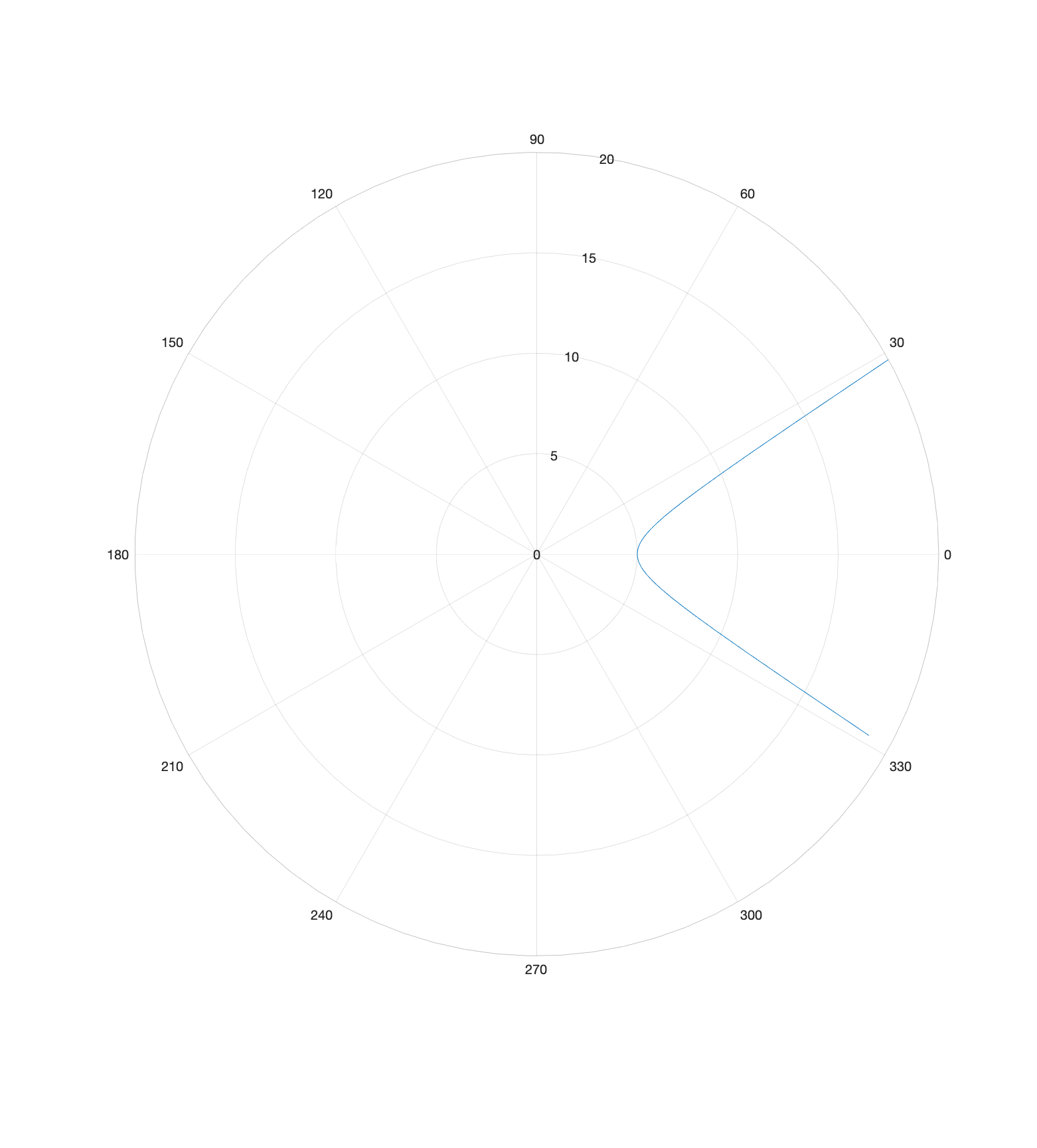
Figure 4: Orbit for $\alpha<0$

We now consider the other cases when $C^{2}+\beta\leq 0$. By differentiating the equation (7) with respect to $t$, we have

$$\ddot{r}-\frac{C^{2}+\beta}{r^{3}}=-\frac{\alpha}{2r^{2}}.$$

Taking the Clairaut variable $\rho=1/r$ and using $C^{2}\dfrac{d^{2}\rho}{d\theta^{2}}=-r^{2}\ddot{r}$, the above equation is transformed into

$$\dfrac{d^{2}\rho}{d\theta^{2}}+\dfrac{C^{2}+\beta}{C^{2}}\rho=\dfrac{\alpha}{2C^{2}}.$$ (14)

When $C^{2}+\beta=0$, the equation reduces to

$$\dfrac{d^{2}\rho}{d\theta^{2}}=\dfrac{\alpha}{2C^{2}}.$$

So, the orbit takes the form

$$\dfrac{1}{r}=\rho=\dfrac{\alpha}{2C^{2}}\theta^{2}+k_{1}\theta+k_{2}$$

which determines a spiral.

When $C^{2}+\beta<0$, the general solution is in the form

$$\dfrac{1}{r}=\rho=k\cos\omega(\theta-g)+\dfrac{\alpha}{2C^{2}},$$

where $\omega=\sqrt{\frac{{C^{2}+\beta}}{C^{2}}}$. Note that in this case $\omega$ is purely-imaginary and thus, the $\cos$ appearing in the above formula is actually a $\cosh$. We may again put it into the form

$$r=\dfrac{p}{1+e\cos\omega(\theta-g)},$$

where $p=\frac{2C^{2}}{\alpha}$ and $e=\frac{2kC^{2}}{\alpha}$. Note that $e$ may be either positive, negative, or zero.

We first discuss the case $\alpha<0$. In this case we have $p<0$ . When $e\geq 0$, there are no solutions. When $-1\leq e<0$, the value of $\theta$ is restricted to $\theta<\theta_{1}\leq\theta_{2}<\theta$ with two limiting values $\theta_{1},\theta_{2}$ such that $r\to\infty$ when $\theta\to\theta_{1}-0$ or $\theta\to\theta_{2}+0$, and $r\to 0$ when $\theta\to\pm\infty$, thus the orbit is an unbounded spiral. When $e<-1$, we have $r<\dfrac{p}{1+e}$ and $r\to 0$ when $\theta\to\pm\infty$, thus the orbit is a bounded spiral biasymptotic to the origin.

Secondly, we discuss the case $\alpha>0$. In this case $p>0$ . When $e>0$, we see that $r\to 0$ when $\theta\to\pm\infty$, so the orbit is a spiral which is biasymptotic to the origin. When $e=0$, the orbit is a circle. When $-1<e<0$, $\theta$ is confronted between two limiting values, and the orbit is unbounded and has two asymptotic directions. There are no solutions when $e\leq-1$.

4.2 Computation of General Boltzmann’s Billiard Mapping

The billiard system is defined by adding a wall of reflection to the central force problem. In this section, we assume $\alpha>0$ and $C^{2}+\beta>0$. We define an arc as part of an orbit with starting and ending points on the reflection wall, and no other points hit the wall in between. The billiard mapping that sends a reflection point and a reflection velocity to the next extends to a mapping that maps an arc to another arc which then extends to a mapping of orbits. We shall analyze this mapping.

In polar coordinates, the wall of reflection $\left\{y=\gamma>0\right\}$ is represented by the equation

$$r\sin\theta=\gamma.$$

We compute the billiard mapping for which a given orbit is reflected after reaching a point $(r_{*},\theta_{*})=(\gamma/\sin\theta_{*},\theta_{*})$ on the wall.

Once fixing the energy, a non-circular, non-singular orbit is characterized by the coordinates $(g,C)$, constructed in Section 2. Define the billiard mapping $S$ as $S(g_{1},C_{1})=(g_{2},C_{2})$, where $(g_{1},C_{1})$ and $(g_{2},C_{2})$ correspond to the orbits before and after the reflection. The derivatives

$$\dfrac{dr}{d\theta}(r_{*},\theta_{*})=\dfrac{p\cdot e\cdot\omega\cdot\sin\omega(\theta_{*}-g_{1,2})}{(1+e\cos\omega(\theta_{*}-g_{1,2}))^{2}}$$

will be denoted as $r^{\prime}_{1,2}$ respectively. The derivatives $\dfrac{d\theta}{dt}(r_{*},\theta_{*})$ will be denoted as $\dot{\theta}_{1,2}$respectively. We also write the corresponding $p,e,\omega$ in the two orbits as $p_{1,2},$ $e_{1,2},$ and $\omega_{1,2}$.

We get the following equations from the law of reflection.

$$\begin{cases}r_{*}=\dfrac{\gamma}{\sin\theta_{*}}=\dfrac{p_{1}}{1+e_{1}\cos\omega_{1}(\theta_{*}-g_{1})}=\dfrac{p_{2}}{1+e_{2}\cos\omega_{2}(\theta_{*}-g_{2})}\\ (r^{\prime}_{1}\sin\theta_{*}+r_{*}\cos\theta_{*})\dot{\theta}_{1}=-(r^{\prime}_{2}\sin\theta_{*}+r_{*}\cos\theta_{*})\dot{\theta}_{2}\\ (r^{\prime}_{1}\cos\theta_{*}-r_{*}\sin\theta_{*})\dot{\theta}_{1}=(r^{\prime}_{2}\cos\theta_{*}{-}r_{*}\sin\theta_{*})\dot{\theta}_{2}\\ \dot{\theta}_{1}=\dfrac{C_{1}}{r_{*}^{2}},\qquad\dot{\theta}_{2}=\dfrac{C_{2}}{r_{*}^{2}}\end{cases}$$

From these we deduce

$$C_{2}=\dfrac{C_{1}(-2r_{*}\cos^{2}\theta_{*}-2r^{\prime}_{1}\sin\theta_{*}\cos\theta_{*}+r_{*})}{r_{*}},$$

$$r^{\prime}_{2}=\dfrac{-r_{*}r^{\prime}_{1}\tan^{2}\theta_{*}-2r_{*}^{2}\tan\theta_{*}+r^{\prime}_{1}r_{*}}{r_{*}\tan^{2}\theta_{*}-2r^{\prime}_{1}\tan\theta_{*}-r_{*}},$$

and

$$p_{2}=\dfrac{2(C_{2}^{2}+\beta)}{\alpha},\quad\omega_{2}=\sqrt{\frac{(C_{2}^{2}+\beta)}{C_{2}^{2}}},\quad e_{2}=\sqrt{1+\frac{8E(C_{2}^{2}+\beta)}{\alpha^{2}}}.$$

Consequently, we obtain

$$e_{2}\cos\omega_{2}(\theta_{*}-g_{2})=\dfrac{p_{2}-r_{*}}{r_{*}},\qquad e_{2}\sin\omega_{2}(\theta_{*}-g_{2})=\dfrac{p_{2}r^{\prime}_{2}}{\omega_{2}r_{*}^{2}}$$

From these we solve $g_{2}$ as

$$g_{2}=\theta_{*}-\frac{\operatorname{sign}\left(\dfrac{p_{2}r^{\prime}_{2}}{e_{2}\omega_{2}r_{*}^{2}}\right)\arccos\left(\dfrac{p_{2}-r_{*}}{e_{2}r_{*}}\right)}{\omega_{2}}.$$ (15)

Remember that, when $\omega\neq 1$, there are multiple pericenters and apocenters. We choose the closest pericenter from the current reflection point, that is defined in (15) as the next argument of pericenter. In order to complete this inductive step, we compute the next reflection point $(r_{**},\theta_{**})$ with $0<\theta_{**}<\pi$ from

$$e_{2}\cos\omega_{2}(\theta_{**}-g_{2})=\dfrac{p_{2}-r_{**}}{r_{**}},\quad r_{**}\sin\theta_{**}=\gamma.$$ (16)

In general, Equation (16) have multiple solutions, with $(r_{*},\theta_{*})$ being one of them. We therefore add the following condition to determine the next reflection point $(r_{**},\theta_{**})$ :

$$r\cdot\sin\theta=\frac{p\sin\theta}{e\cos(\omega(\theta-g))-1}\geq\gamma$$ (17)

for all $\theta$ such that $\theta_{*}\leq\theta\leq\theta_{**}$ if $C>0$ (for all $\theta$ such that $\theta_{**}\leq\theta\leq\theta_{*}$ if $C<0$).

4.3 Solutions of the Central Force Problem: The Case of Cotes’ Spirals

We here consider the case $\alpha=0,{\beta\neq 0},C\neq 0$, in this special case, solution curves of the central force problem with a force function $\beta/r^{2}$ are Cotes’ spiral [2, Chapter IV].

Differentiating the equation (7) with respect to $t$, we have

$$\ddot{r}-\frac{C^{2}+\beta}{r^{3}}=-\frac{\alpha}{2r^{2}}.$$

Taking the Clairaut variable $\rho=1/r$ and having $C^{2}\dfrac{d^{2}\rho}{d\theta^{2}}=-r^{2}\ddot{r}$, the above equation is transformed into

$$\dfrac{d^{2}\rho}{d\theta^{2}}+\dfrac{C^{2}+\beta}{C^{2}}\rho=\dfrac{\alpha}{2C^{2}}.$$ (18)

By substituting $\alpha=0$, the equation (18) can be written into

$$\dfrac{d^{2}\rho}{d\theta^{2}}+\left(\dfrac{C^{2}+\beta}{C^{2}}\right)\rho=0.$$

We discuss different subcases.

When $C^{2}+\beta>0$, the general solution of the equation is written as

$$\dfrac{1}{r}=\rho=k\cos{\omega(\theta-\psi)},$$

where $k\in\mathbb{R}$ and $\psi\in[0,2\pi)$. When $C^{2}+\beta=0$, the general solution reduces to the form

$$\dfrac{1}{r}=\rho=k_{1}\theta+k_{2}.$$

When $C^{2}+\beta<0$, the general solution is

$$\dfrac{1}{r}=\rho=k_{1}\exp\left({i\omega(\theta-\psi}\right)+k_{2}\exp\left({-i\omega(\theta-\psi)}\right),$$

with a purely imaginary $\omega$.

To make further analysis observe that

$$h:=\left(\dfrac{d\rho}{d\theta}\right)^{2}+\left(\dfrac{C^{2}+\beta}{C^{2}}\right)\rho^{2}$$

is a first integral of the equation. Drawing its level sets in the phase space with coordinates $\bigl{(}\dfrac{d\rho}{d\theta},\rho\bigr{)}$, we see that the level sets are hyperbolae and bifurcate at the zero-level $\left\{h=0\right\}$ through a degeneration into a pair of lines, and then continue as hyperbolae with the major axis switched.

When $h<0$, the hyperbola has the $\rho-$axis as major axis and admits a parametrization with hyperbolic functions. The corresponding solution in polar form is

$$\dfrac{1}{r}=\rho=k\cos\omega(\theta-\psi).$$

Similarly, when $h>0$, we get

$$\dfrac{1}{r}=\rho=k\cdot i\cdot\sin\omega(\theta-\psi).$$

And, when $h=0$ we have

$$\dfrac{1}{r}=\rho=k\exp\left(\pm i\omega(\theta-\psi)\right).$$

We thus get the five classes of Cotes’ spirals as orbits of the problem with $\alpha=0$.

4.4 Computation of the Billiard Mapping: Cotes’ Spiral Case

We here compute the billiard mapping for the special case $\alpha=0$. We again only consider bounded orbits, thus we assume $E<0$.

The doubled total energy is written as

$${2E=}\,\dot{r}^{2}+\frac{C^{2}+\beta}{r^{2}},$$

which leads to

$$h=\left(\dfrac{d\rho}{d\theta}\right)^{2}+(\dfrac{C^{2}+\beta}{C^{2}})\rho^{2}=\frac{2E}{C^{2}}{<0}.$$

Thus $C^{2}+\beta<0$ and

the orbits are given in the form

$$\dfrac{1}{r}=\rho=k\cos\omega(\theta-\psi).$$

with $\omega=\sqrt{\frac{C^{2}+\beta}{C^{2}}},k=\sqrt{\frac{2E}{\omega^{2}C^{2}}}$ and $\psi$ the argument of the apocenter.

We consider the billiard mapping $(\psi_{1},C_{1})\mapsto(\psi_{2},C_{2})$. Let $(r_{*},\theta_{*})$ be the reflection point. The derivatives

$$\dfrac{dr}{d\theta}(r_{*},\theta_{*})=\dfrac{\omega\sin\omega(\theta_{*}-\psi_{1,2})}{k\cos^{2}\omega(\theta_{*}-\psi_{1,2})}$$

are denoted as $r^{\prime}_{1,2}$ respectively. The derivatives $\dfrac{d\theta}{dt}(r_{*},\theta_{*})$ are denoted as $\dot{\theta}_{1,2}$ respectively. We also write the corresponding $p,e,\omega$ in the two orbits as $p_{1,2},$ $e_{1,2},$ and $\omega_{1,2}$. The next reflection point is computed using the following equations

$$\begin{cases}r_{*}=\dfrac{\gamma}{\sin\theta_{*}}=\dfrac{1}{k_{1}\cos\omega_{1}(\theta_{*}-\psi_{1})}=\dfrac{1}{k_{2}\cos\omega_{2}(\theta_{*}-\psi_{2})}\\ (r^{\prime}_{1}\sin\theta_{*}+r_{*}\cos\theta_{*})\dot{\theta}_{1}=-(r^{\prime}_{2}\sin\theta_{*}+r_{*}\cos\theta_{*})\dot{\theta}_{2}\\ (r^{\prime}_{1}\cos\theta_{*}-r_{*}\sin\theta_{*})\dot{\theta}_{1}=(r^{\prime}_{2}\cos\theta_{*}{-}r_{*}\sin\theta_{*})\dot{\theta}_{2}\\ \dot{\theta}_{1}=\dfrac{C_{1}}{r_{*}^{2}},\qquad\dot{\theta}_{2}=\dfrac{C_{2}}{r_{*}^{2}}.\end{cases}$$

From these one deduces that

$$C_{2}=\dfrac{C_{1}(-2r_{*}\cos^{2}\theta_{*}-2r^{\prime}_{1}\sin\theta_{*}\cos\theta_{*}+r_{*})}{r_{*}},$$

$$r^{\prime}_{2}=\dfrac{-r_{*}r^{\prime}_{1}\tan^{2}\theta_{*}-2r_{*}^{2}\tan\theta_{*}+r^{\prime}_{1}r_{*}}{r_{*}\tan^{2}\theta_{*}-2r^{\prime}_{1}\tan\theta_{*}-r_{*}},$$

and then

$$\omega_{2}=\sqrt{\frac{C_{2}^{2}+\beta}{C_{2}^{2}}},$$

$$k_{2}=\sqrt{\frac{2E}{\omega_{2}^{2}C_{2}^{2}}}.$$

Consequently, we obtain

$$\frac{1}{r_{*}}=k_{2}\cos\omega_{2}(\theta_{*}-\psi_{2}),\quad-\frac{1}{r_{*}^{2}}r^{\prime}_{2}=-k_{2}\omega_{2}\sin\omega(\theta_{*}-\psi_{2}).$$

Thus $\psi_{2}$ can be solved as

$$\psi_{2}=\theta_{*}-\frac{\operatorname{sign}\left(-\frac{r^{\prime}_{2}}{r_{*}k_{2}(-i\omega)}\right)\operatorname{arccosh}\left(\frac{1}{k_{2}r_{*}}\right)}{-i\omega_{2}}.$$

The next reflection point $(r_{**},\theta_{**})$, $0<\theta_{**}<\pi$ is then computed from

$$\frac{1}{r_{**}}=k_{2}\cos\omega_{2}(\theta_{**}-\psi_{2}),\quad r_{**}\sin\theta_{**}=\gamma.$$ (19)

5 Numerical Results of Boltzmann’s Billiard Trajectories

We here present some numerical simulations of Boltzmann’s billiard mapping based on Section 4.2. In our simulations, we set $\alpha=4,E=-0.5,\gamma=0.5$, and vary the parameter $\beta\geq 0$. Figures in this section illustrate numerically computed trajectories of the billiard mapping i.e. the evolving values of

$$(g,C)\in[0,2\pi)\times[C_{min},C_{max}]$$

at each reflection. All numerical computations here have been operated by MATLAB and the interval arithmetic [9] has been used to count the solutions satisfying Equation (16) or (19).

For $\beta=0$, our simulation shows periodic behavior of a trajectory as we illustrated in Figure 5, which is compatible with the integrability of the system For small $\beta$, for example $\beta=0.5$ the system remains quasi-periodicity and seems not to be transitive, see figure 6. For a bigger value of $\beta$, the (quasi-)periodicity may break, and chaotic behavior appears, as we illustrated for the case $\beta=2.6$ in Figure 7. In this case, it seems possible that a single orbit densely covers the whole energy hypersurface. Therefore for big enough $\beta$, it is possible to have ergodic systems. However, chaotic behavior does not always show up for large $\beta$. Figure 8 shows both quasi-periodic (Subfig. a) and chaotic (but not transitive) behavior (Subfig. b) for $\beta=2.4$, with different initial values. Subfig. c indicates the existence of 2-period orbit for this parameter setting.

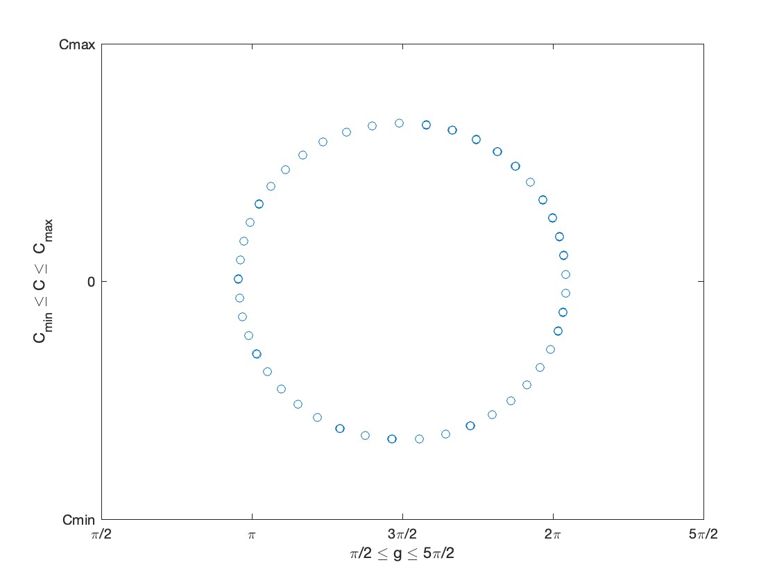
Figure 5: Periodic behavior of the mapping trajectory for $\beta=0$

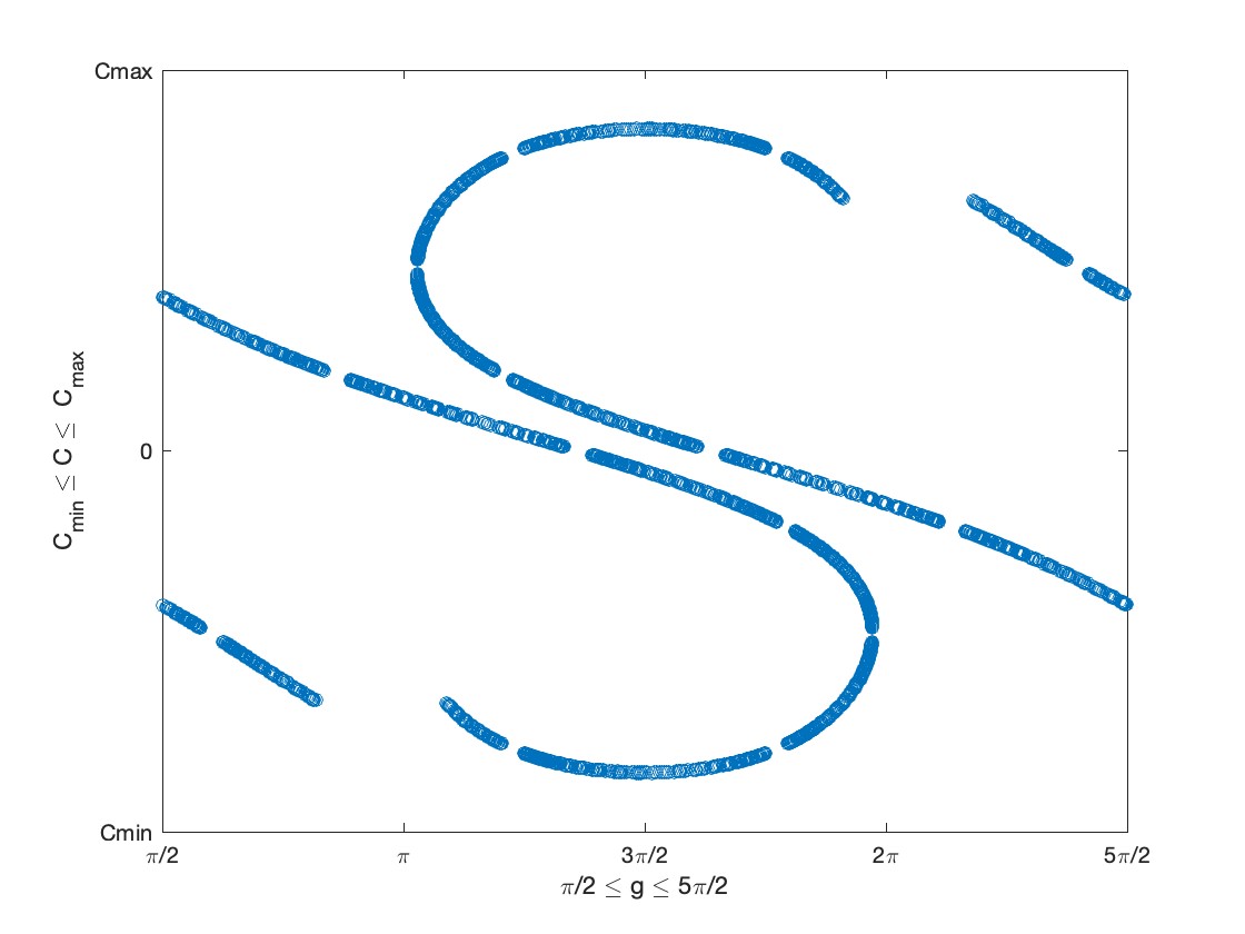
Figure 6: (Quasi-)periodic behavior of the mapping trajectory for $\beta=0.5$

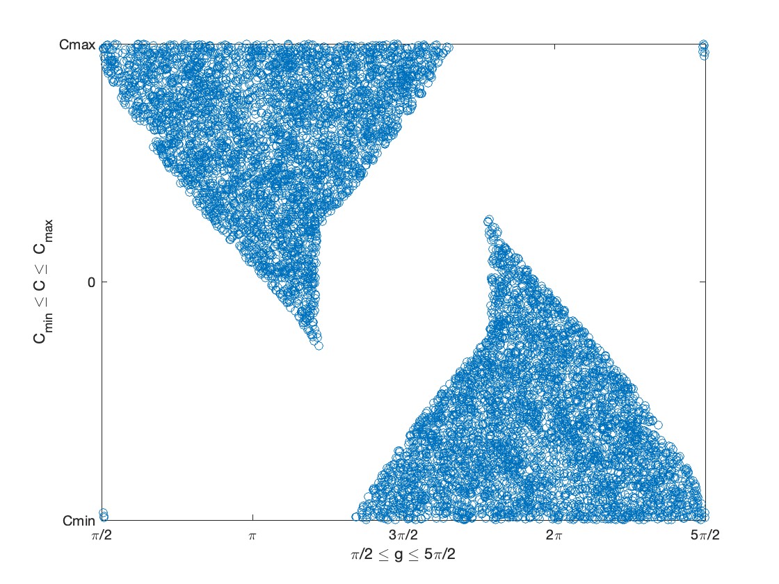
a. Trajectory with initial value $(g_{0},C_{0})=(0.2,0.8)$

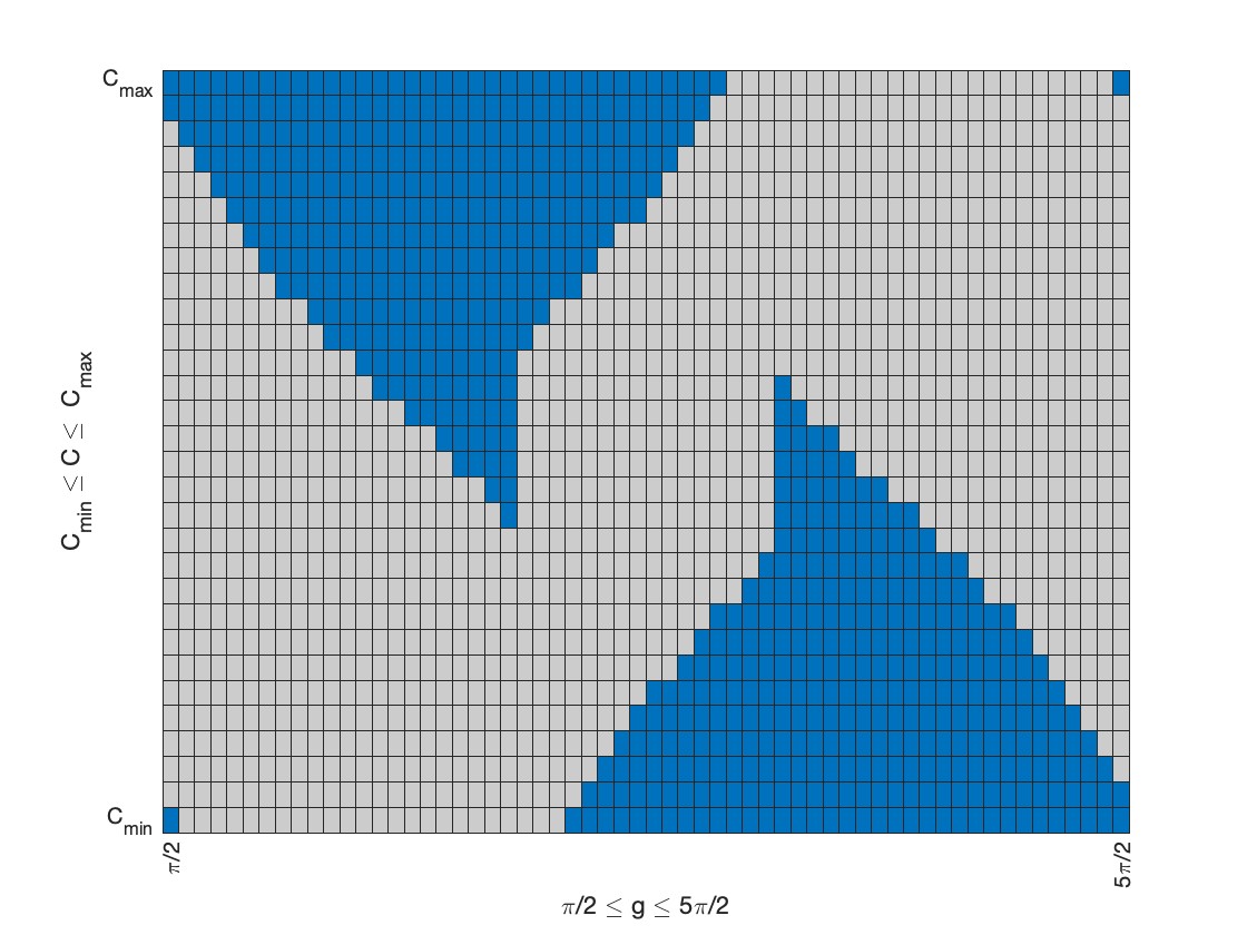
b. Discretized allowed region (in blue)

Figure 7: Transitive behavior of the mapping trajectory for $\beta=2.6$

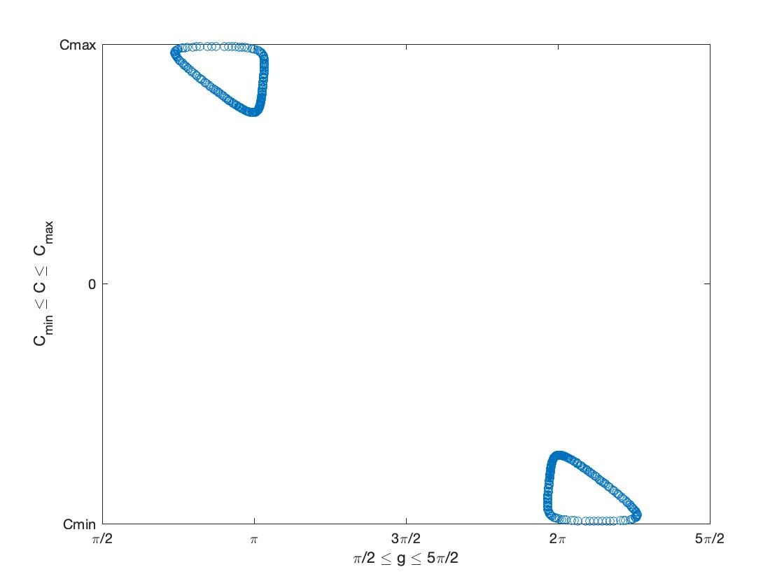
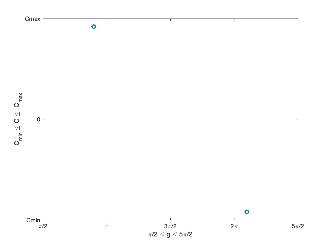
a. Trajectory with initial value $(g_{0},C_{0})=(0.1,1.1)$                c. Periodic trajectory with initial value $(g_{0},C_{0})=(3.45,-1.16)$

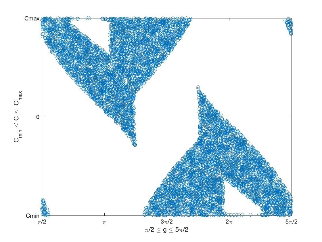
b. Trajectory with initial value $(g_{0},C_{0})=(0.2,1.0)$

Figure 8: (Quasi-)periodic and chaotic behavior for $\beta=2.4$

6 The Koopman Operator and Its Eigenvalue Problem

For any measure-preserving map $S$ on a probability measure space $(X,\mu,\Sigma)$, the Koopman operator can be defined as the transfer operator on $L^{2}(X):=L^{2}(X,{\mu;}\,\mathbb{C})$ by

$$Kf:=f\circ S,\qquad f\in L^{2}(X).$$ (20)

Since $S$ is measure preserving, the Koopman operator $K:L^{2}(X)\to L^{2}(X)$ is unitary and has its spectrum on the unit circle. The spectrum of the Koopman operator carries essential dynamical information of the map $S$. In particular, we have

Proposition 1.

Let $S$ be a measure-preserving map on a probability measure space $(X,\mu,\Sigma)$ and let $K:L^{2}(X)\to L^{2}(X)$ be the corresponding Koopman operator. Then $1$ is an eigenvalue of $K$. Moreover, the map $S$ is ergodic if and only if eigenvalue 1 is simple.

See [3, Proposition 7.15] for the proof.

In the following, we numerically investigate the eigenvalue problem of the Koopman operator with the Galerkin method. All numerical computations here have been operated by MATLAB and the interval arithmetic [9] has been used to count the solutions satisfying Equation (16).

6.1 Approximation of Koopman Eigenvalue Problem with Galerkin Method

We here explain the approximation procedure of the Koopman eigenvalue problem using Galerkin method [4] with piecewise constant basis functions.

Galerkin Method and Midpoint Quadrature with Uniform Weights

Consider the original eigenvalue problem of the Koopman operator on $L^{2}(X)$

$$Ku=\lambda u,\qquad u\in L^{2}(X),$$

which can be transformed into the equivalent equation

$$\langle Ku,v\rangle=\lambda\langle u,v\rangle,\qquad\forall v\in L^{2}(X),$$

where $\langle\cdot,\cdot\rangle$ is the inner product of the Hilbert space $L^{2}(X)$. We fix finitely many basis functions $\{f_{1},\cdots,f_{N}\}$ in $L^{2}(X)$. We look for approximate eigenfunctions in the form $u=\sum_{n=1}^{N}\alpha_{i}f_{i}$ and we restrict the above equation to the space which is spanned by the base functions. Then we have

$$\sum_{n=1}^{N}\alpha_{n}\langle f_{n}\circ S,f_{m}\rangle=\lambda\sum_{n=1}^{N}\alpha_{n}\langle f_{n},f_{m}\rangle,\qquad\forall m\in\{1,\cdots,N\}.$$

In matrix form this is

$$\begin{pmatrix}\langle f_{1}\circ S,f_{1}\rangle&\cdots&\langle f_{N}\circ S,f_{1}\rangle\\ \\ \vdots&\ddots&\vdots\\ \\ \langle f_{1}\circ S,f_{N}\rangle&\cdots&\langle f_{N}\circ S,f_{N}\rangle\end{pmatrix}\begin{pmatrix}\alpha_{1}\\ \\ \vdots\\ \\ \alpha_{N}\end{pmatrix}=\lambda\begin{pmatrix}\langle f_{1},f_{1}\rangle&\cdots&\langle f_{N},f_{1}\rangle\\ \\ \vdots&\ddots&\vdots\\ \\ \langle f_{1},f_{N}\rangle&\cdots&\langle f_{N},f_{N}\rangle\end{pmatrix}\begin{pmatrix}\alpha_{1}\\ \\ \vdots\\ \\ \alpha_{N}\end{pmatrix}$$ (21)

.

For the computation of each entry of the matrices above, we divide the domain $X$ of the mapping $S$ into finitely many disjoint regions $\Omega_{1},\cdots\Omega_{N}$ so that $X=\sqcup_{n=1}^{N}\Omega_{n}$. Suppose that our basis functions $f_{n}$ are the characteristic functions of each region $\Omega_{n}$ i.e. $f_{n}(x)=1$ if $x\in\Omega_{n}$ and $f_{n}(x)=0$ otherwise. Then the matrix in the left hand side of (21) can be written as

$$\begin{split}\langle f_{n}\circ S,f_{m}\rangle&=\int_{X}f_{n}(S(x))\cdot f_{m}(x)dx\\ &=\int_{\Omega_{m}}f_{n}(S(x))dx\\ &\approx\sum_{\ell=1}^{L}w_{\ell}^{(m)}f_{n}(S(x_{\ell}))\end{split}$$ (22)

In the last line, we approximated the integral with the weighted summation of $f_{n}(S(x_{\ell}))$ over $L$ nodes in $\Omega_{m}$ which is chosen by the midpoint rule.

If we set the same weight $w^{(m)}=w_{\ell}^{(m)}$ at all nodes $\{x_{\ell}\}_{\ell=1}^{L}$ in $\Omega_{m}$, then we can simplify the above formula as

$$\begin{split}\langle f_{n}\circ S,f_{m}\rangle&\approx\sum_{\ell=1}^{L}w_{\ell}^{(m)}f_{n}(S(x_{\ell}))\\ &=w^{(m)}\cdot\#\{\ell\mid S(x_{\ell})\in\Omega_{n}\}\\ &=|\Omega_{m}|\cdot\frac{\#\{\ell\mid S(x_{\ell})\in\Omega_{n}\}}{L},\end{split}$$ (23)

where $|\Omega_{m}|$ is the measure of $\Omega_{m}$. In the last equation, we used

$$|\Omega_{m}|=\int_{\Omega_{m}}dx=\sum_{\ell~{}\text{s.t.}x_{\ell}\in\Omega_{m}}w_{\ell}^{(m)}=\#\{\ell\mid x_{\ell}\in\Omega_{m}\}\cdot w^{(m)}=L\cdot w^{(m)}.$$

The matrix in the left hand side of (21) becomes

$$\langle f_{n},f_{m}\rangle =\int_{\Omega}f_{n}(x)\cdot f_{m}(x)dx$$

$$=\int_{\Omega_{m}}f_{n}(x)dx$$

$$\approx\sum_{\ell=1}^{L}w_{\ell}^{(m)}f_{n}(x_{\ell})$$

$$=w^{(m)}\cdot\#\{\ell\mid x_{\ell}\in\Omega_{n}\}$$

$$=\begin{cases}|\Omega_{n}|\qquad\text{if $n=m$}\\ 0\qquad\text{otherwise.}\end{cases}$$

We call the matrix eigenvalue problem (21) approximated in the above way the discretized Koopman eigenvalue problem.

We now set $X=[0,2\pi)\times[C_{min},C_{max}]$, $x=(g,C)\in X$ and let $S$ be Boltzmann’s billiard mapping computed in Section 4 and consider the approximated eigenvalue problem of the corresponding Koopman operator.

In the following numerical computations, we divided the $(g,C)-$coordinate space $[0,2\pi)\times[C_{min},C_{max}]$ into $N=800$ partial sets. The number $L=25$ represents the number of the test nodes in each section used to approximate integrals, which appear in the equations (22) and (23). We note that the billiard mapping $S$ is not defined on the whole space $[0,2\pi)\times[C_{min},C_{max}]$, therefore we need to restrict the divided space into the subset of all partitions where the corresponding orbits of the underlying mechanical system have at least two intersection points with the reflection wall $y=\gamma$ In our computations, we set $\alpha=4.0,E=-0.5,\gamma=0.5$, and vary the parameter $\beta$.

In Figure 9, Subfig. a shows the restricted region in a divided space $[0,2\pi)\times[C_{min},C_{max}]$ where the billiard mapping is well-defined for $\alpha=4.0,\beta=0.0$, and Subfig, b shows the all eigenvalues of the discretized Koopman eigenvalue problem, Subfig. c,d,e, and f show the level sets of all independent eigenfunctions corresponding to the three closest eigenvalues from 1. Figure. 10, Figure. 11 and Figure. 13 show the same information on the discretized Koopman eigenvalue problem as Figure. 9 but for the different parameter setting $\beta=0.5,\beta=2.4$, and $\beta=2.6$, respectively.

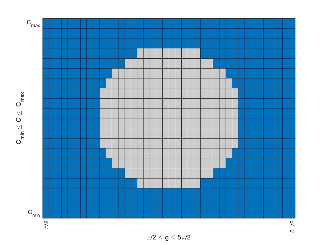
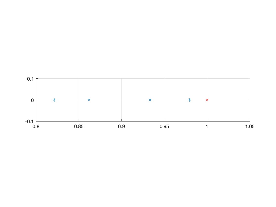
a. Allowed regions (in blue) b. Approximated eigenvalues near $1$

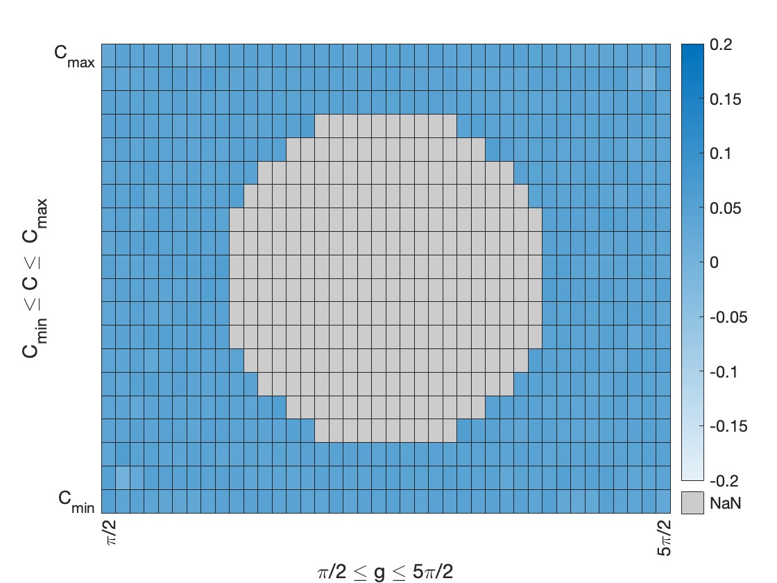
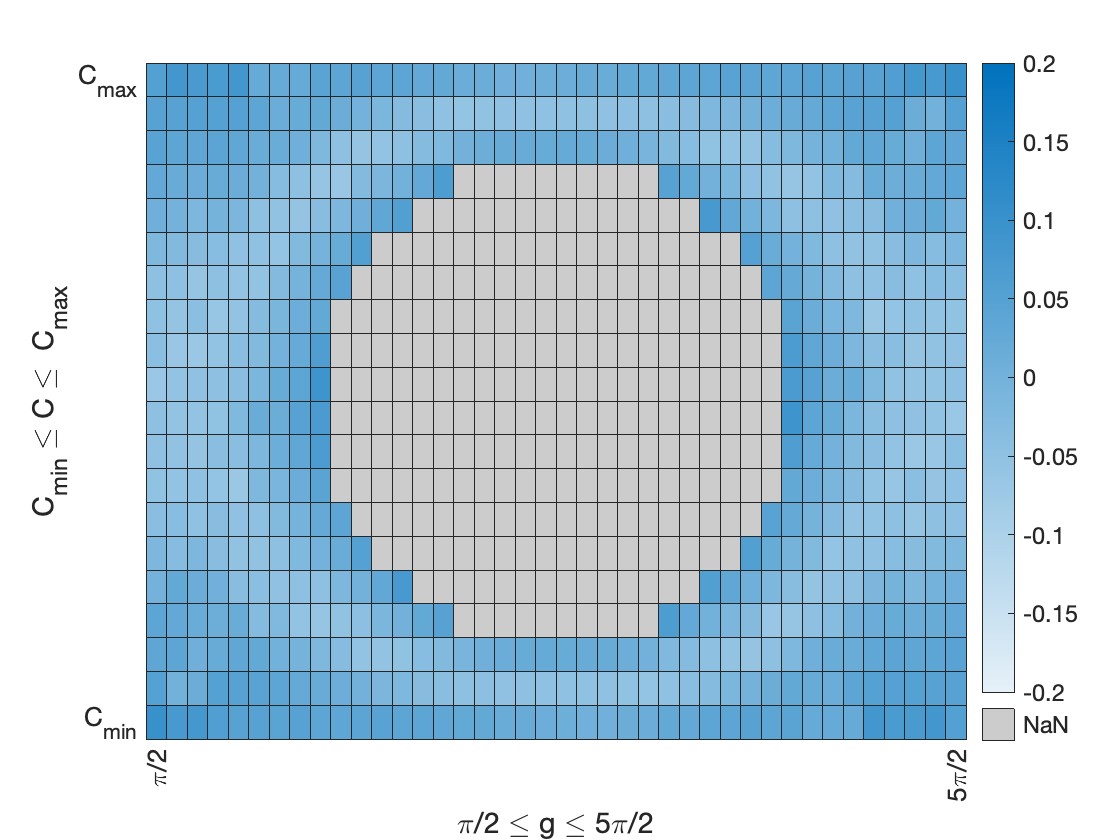
c. Eigenfunction for eigenvalue 1.00 e. Eigenfunction for eigenvalue 0.93

d. Eigenfunction for eigenvalue 0.98

Figure 9: Shifted allowed regions in $(g,C)-$coordinates space $[\pi/2,5\pi/2)\times[C_{min},C_{max}]$. Eigenvalues and eigenfunctions of approximated Koopman operator for $\alpha=4.0,\beta=0.0,N=800,L=25$, uniform weights.

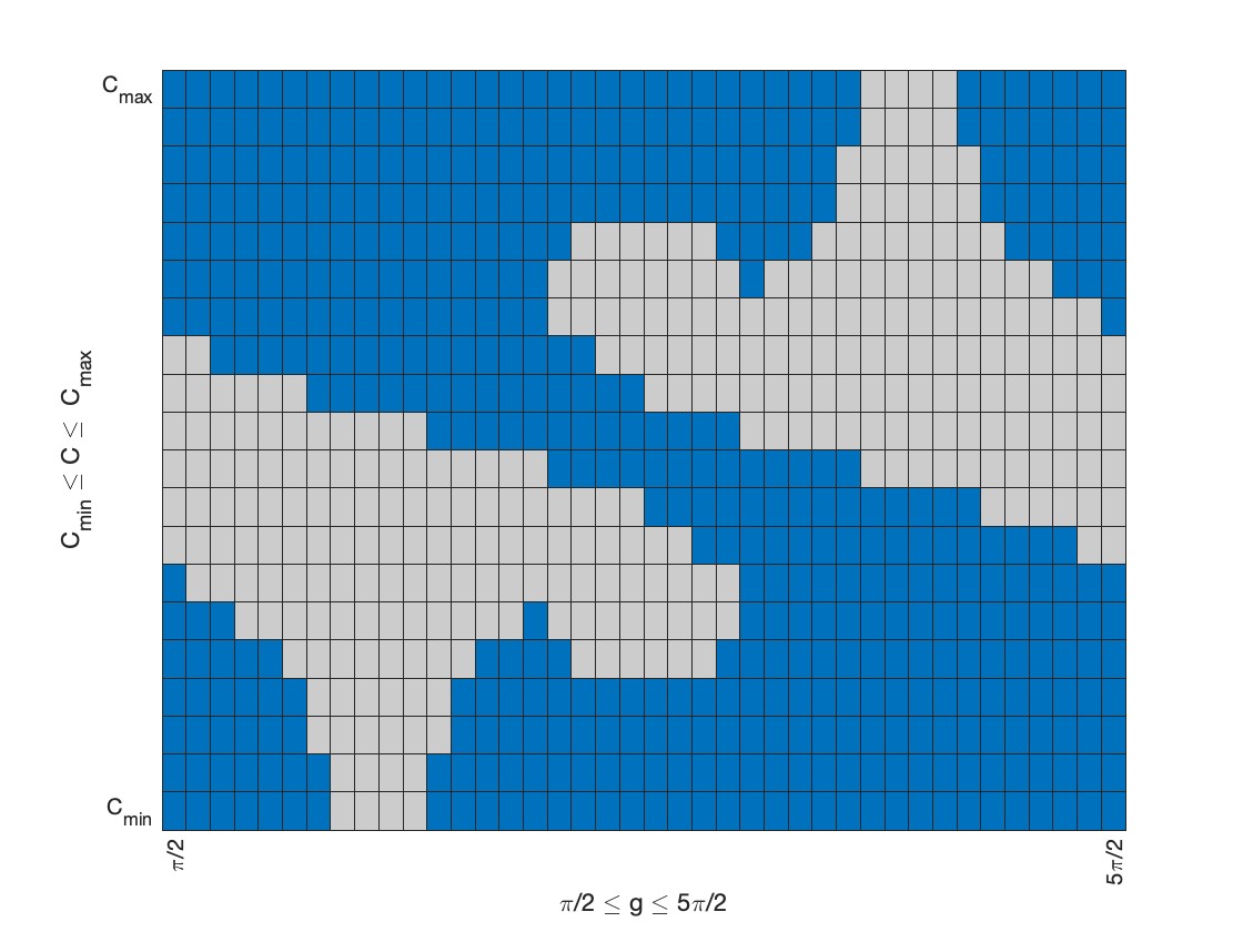
a. Allowed regions (in blue) b. Approximated eigenvalues near $1$

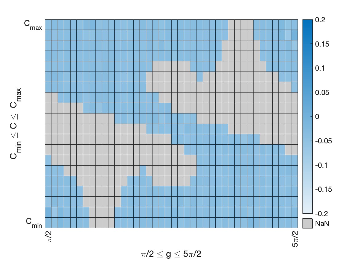
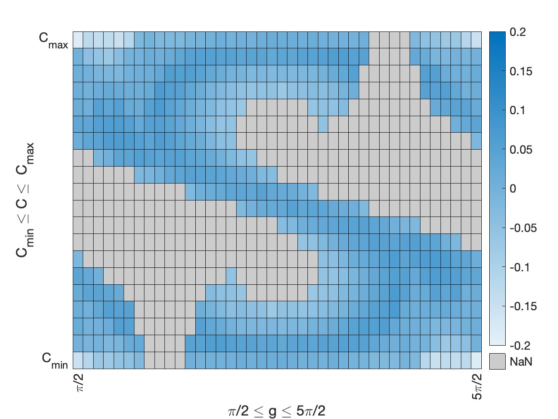
c. Eigenfunction for eigenvalue 1.00 e. Eigenfunction for eigenvalue 0.90

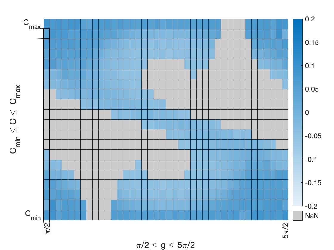
d. Eigenfunction for eigenvalue 0.98

Figure 10: Allowed regions in $(g,C)-$coordinates space $[0,2\pi)\times[C_{min},C_{max}]$. Eigenvalues and eigenfunctions of approximated Koopman operator for $\alpha=4.0,\beta=0.5,N=800,L=25$, uniform weights.

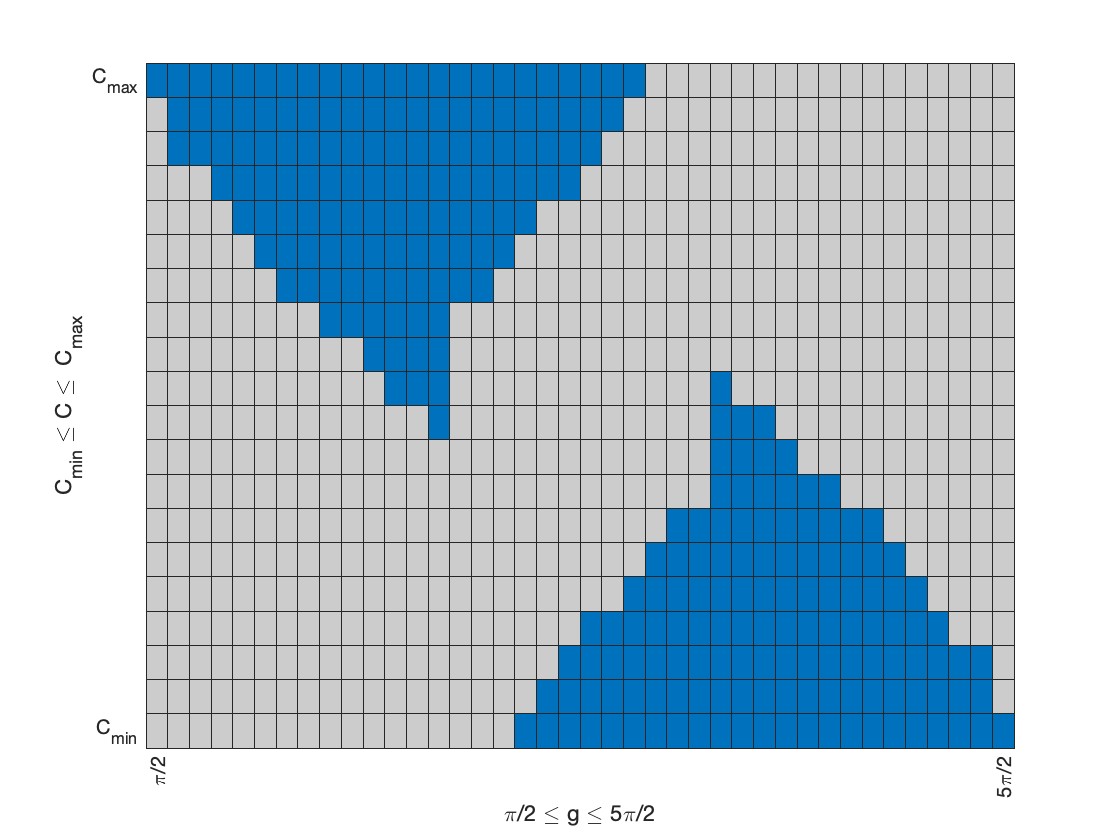
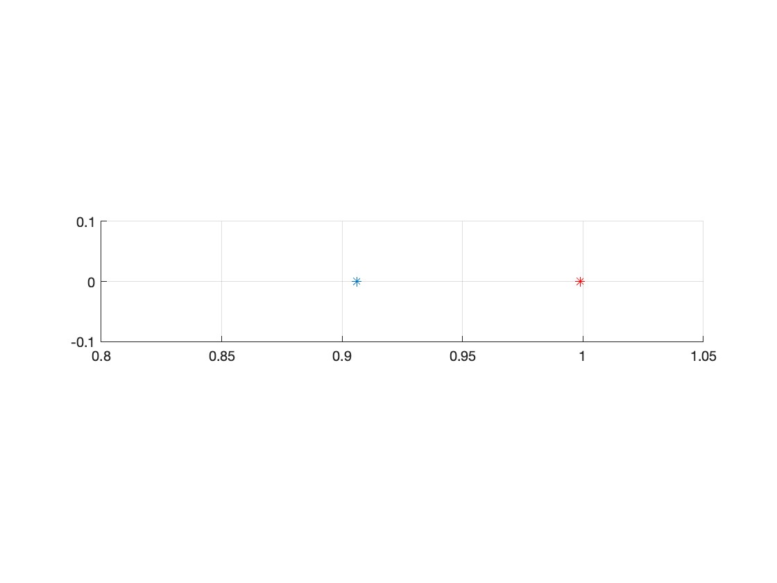
a. Allowed regions (in blue) b. Approximated eigenvalues near $1$

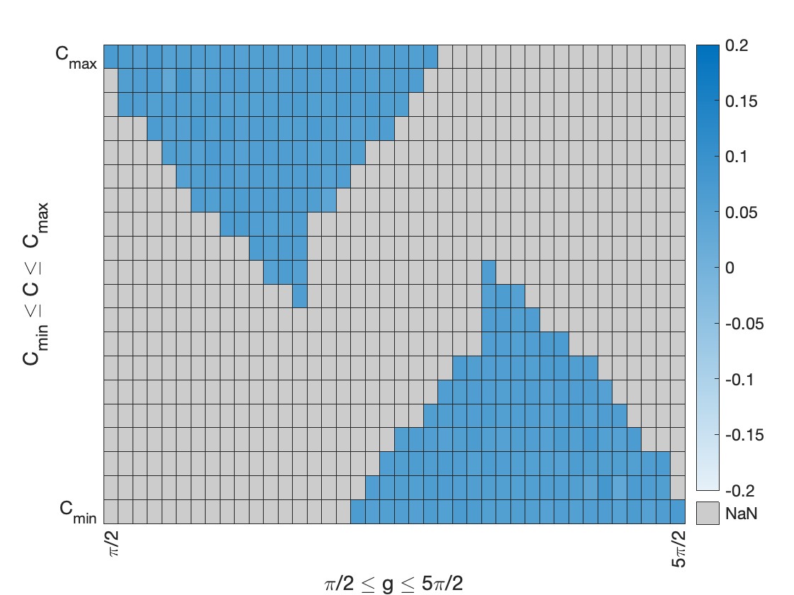
c. Eigenfunction for eigenvalue 1.00

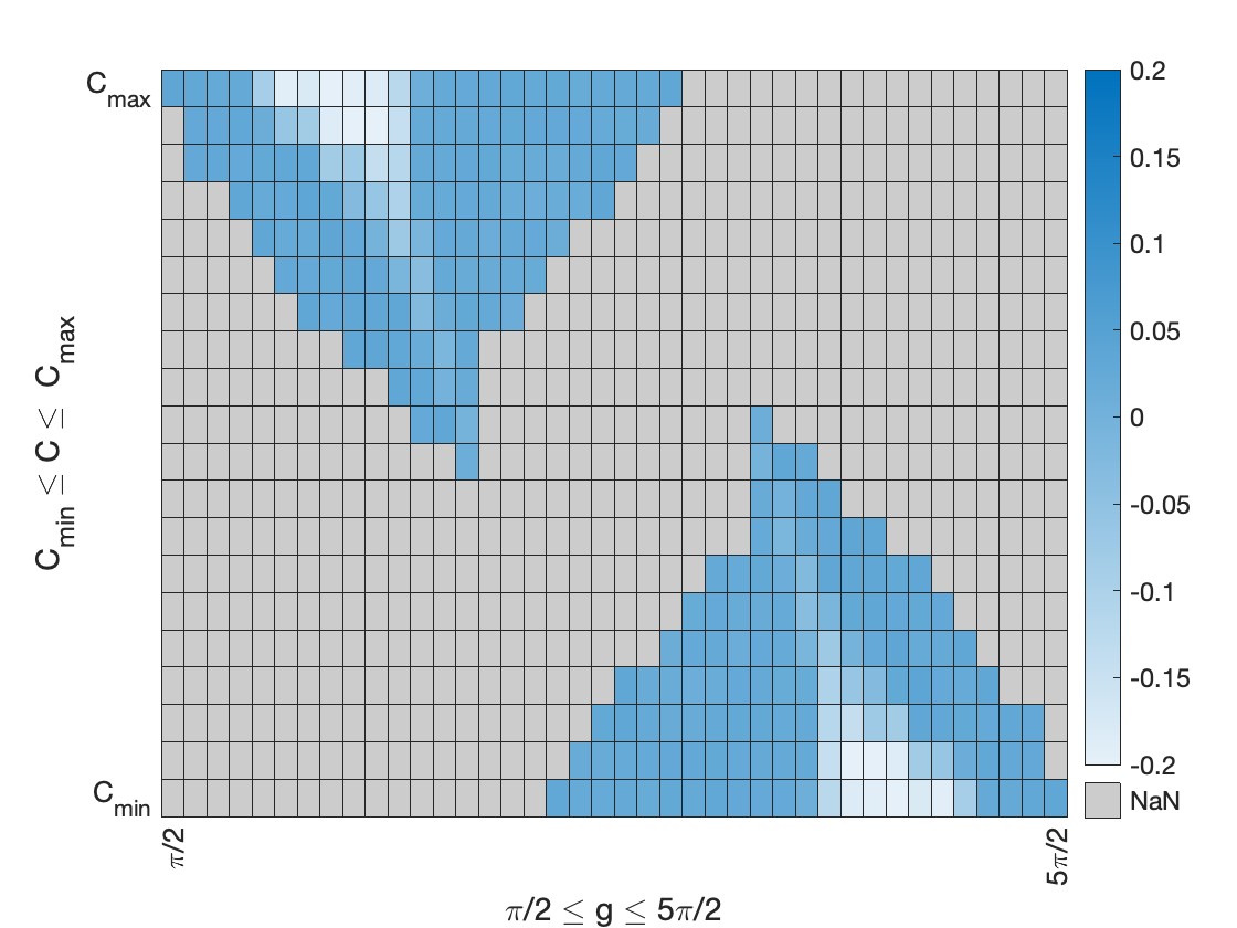
d. Eigenfunction for eigenvalue 0.91

Figure 11: Allowed regions in $(g,C)-$coordinates space $[0,2\pi)\times[C_{min},C_{max}]$. Eigenvalues and eigenfunctions of approximated Koopman operator for $\alpha=4.0,\beta=2.4,N=800,L=25$, uniform weights.

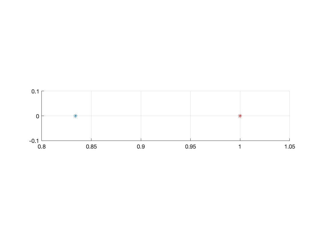
Figure 12: Approximated eigenvalues near $1$ for $\alpha=4.0,\beta=2.4,L=25$, $N=200(\text{left}),800(\text{middle}),1800(\text{right}),$ uniform weights.

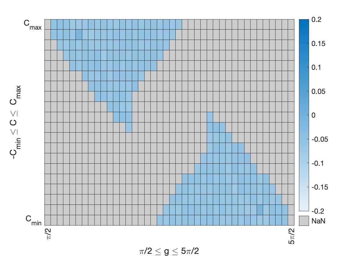
a. Allowed regions (in blue) c. Eigenfunction for eigenvalue 1.00 b. Approximated eigenvalues near $1$

Figure 13: Allowed regions in $(g,C)-$coordinates space $[0,2\pi)\times[C_{min},C_{max}]$. Eigenvalues and eigenfunctions of approximated Koopman operator for $\alpha=4.0,\beta=2.6,N=800,L=25$, uniform weights.

Galerkin method and Gauss-Legendre quadrature

The Gauss-Legendre quadrature approximates the integral of the function $f$ in the domain $[-1,1]$ with the sum of the values of the function at the Gauss points $\{x_{k}\}$, with the appropriate weights $\{w_{k}\}$, as

$$\int_{-1}^{1}f(x)dx\approx\sum_{k=1}^{K}w_{k}f(x_{k}).$$

The Gauss node points can be defined as the roots of the Legendre polynomials

$$P_{K}(x)=\frac{1}{2^{K}K!}\frac{d^{K}}{dx^{K}}(x^{2}-1)^{K},$$

and the weights are assigned as:

$$w_{k}=\frac{2}{(1-x_{k}^{2})[P_{K}^{\prime}(x_{k})]^{2}}.$$

The Gauss-Legendre quadrature can be extended to integration over a surface as:

$$\int_{-1}^{1}\int_{-1}^{1}f(x,y)dx_{1}dx_{2}\approx\sum_{k_{1}=1}^{K}\sum_{k_{2}=1}^{K}w_{k_{1}k_{2}}f(x_{k},x_{l}),$$

where $w_{k_{1}k_{2}}=w_{k_{1}}w_{k_{2}}$. In this way, we approximate each entry of the matrices in (21) and get

$$\begin{split}\langle f_{n}\circ S,f_{m}\rangle&=\int_{X}f_{n}(S(x))\cdot f_{m}(x)dx\\ &=\int_{\Omega_{m}}f_{n}(S(x))dx\\ &\approx\sum_{k_{1}=1}^{K}\sum_{k_{2}=1}^{K}a_{m}w_{k_{1}k_{2}}^{(m)}f_{n}(S(x_{k_{1}k_{2}})\\ &=\sum_{\ell=1}^{L=K\times K}w_{\ell}^{(m)}f_{n}(S(x_{\ell}))\\ &=\sum_{\ell~{}\text{s.t.}S(x_{\ell})\in\Omega_{n}}w_{\ell}^{(m)},\end{split}$$ (24)

where $a_{m}$ is the area of $\Omega_{m}$ and $w^{(m)}_{\ell}:=a_{m}w^{(m)}_{k_{1}k_{2}}$ and

$$\begin{split}\langle f_{n},f_{m}\rangle&=\int_{X}f_{n}(x)\cdot f_{m}(x)dx\\ &=\int_{\Omega_{m}}f_{n}(x)dx\\ &\approx\sum_{\ell=1}^{L}w_{\ell}^{(m)}f_{n}(x_{\ell})\\ &=\sum_{\ell~{}\text{s.t.}x_{\ell}\in\Omega_{n}}w_{\ell}^{(m)}.\end{split}$$ (25)

Remind that $f_{n}(x_{\ell})=1$ if $x_{\ell}\in\Omega_{n}$ and $f_{n}(x_{\ell})=0$ otherwise.

We again set $X=[0,2\pi)\times[C_{min},C_{max}]$, $x=(g,C)$ and consider the approximated eigenvalue problem of the corresponding Koopman operator with the Galerkin method using the Gauss-Legegendre quadrature.

In the following numerical computations, we divided $X$ into $N=800$ partial sets. Recall that we need to restrict the space $[0,2\pi)\times[C_{min},C_{max}]$ into the subset where the billiard mapping is well-defined. In our computations, we set $\alpha=4.0,E=-0.5,\gamma=0.5$, and vary the parameter $\beta$. The number $L=25$ represents the number of Gauss nodes in each partition used to approximate integrals, which appear in the equations (24) and (25).

In the following figures, we illustrate the numerical results.

In Figure 14, Subfig. a shows the restricted region in a divided phase space $[0,2\pi)\times[C_{min},C_{max}]$ ($N=800$) where the billiard mapping is well-defined for $\alpha=4.0,\beta=0.0$, Subfig. b shows the all eigenvalues of the discretized Koopman eigenvalue problem, and Subfig. c, d, e, and f show the level sets of all independent eigenfunctions corresponding to the three closest eigenvalues from 1. Figure 15, Figure 16 and Figure 17 show the numerical results for $\beta=0.5,\beta=2.4$ and $\beta=2.6$, respectively.

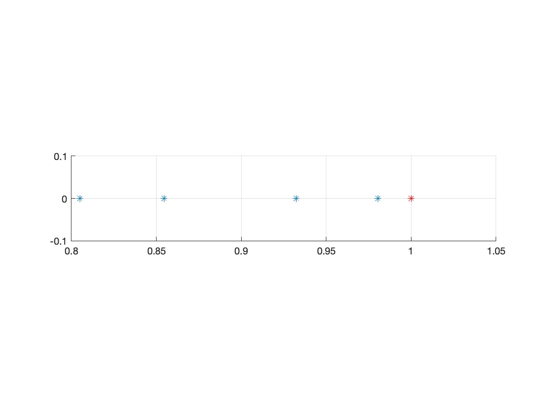
a. Allowed regions (in blue) b. Approximated eigenvalues near $1$

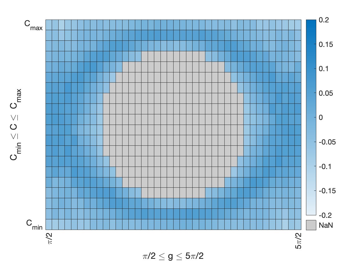
c. Eigenfunction for eigenvalue 1.00 e. Eigenfunction for eigenvalue 0.93

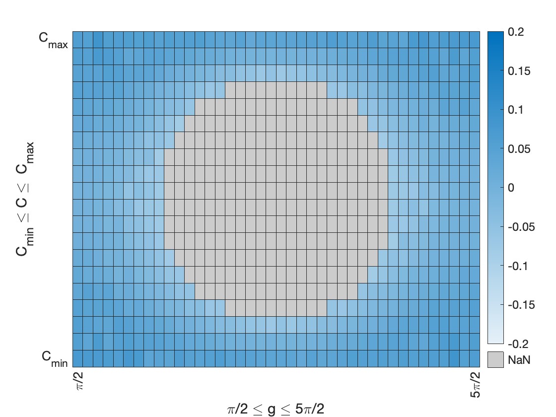
f. Eigenfunction for eigenvalue 0.98

Figure 14: Allowed regions in $(g,C)-$coordinates space $[0,2\pi)\times[C_{min},C_{max}]$. Eigenvalues and eigenfunctions of approximated Koopman operator for $\alpha=4.0,\beta=0.0,N=800,L=25$, Gauss-Legendre quadrature.

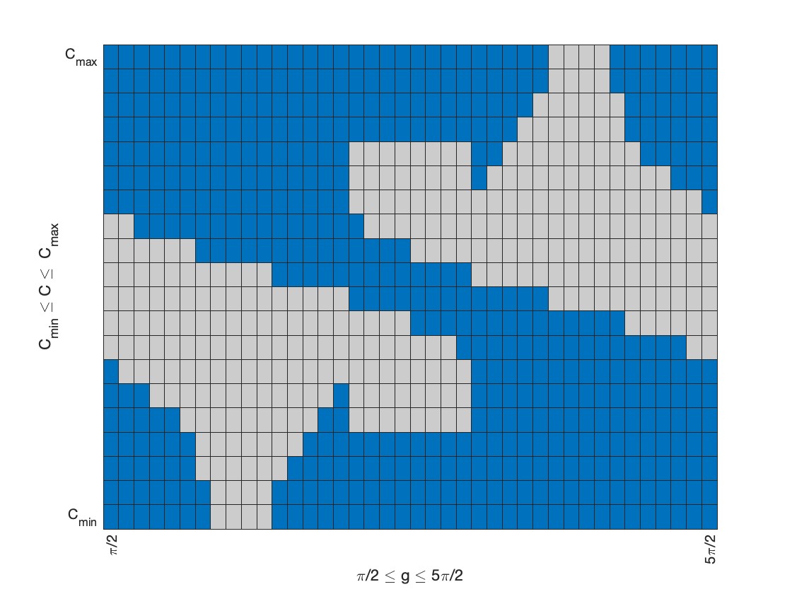
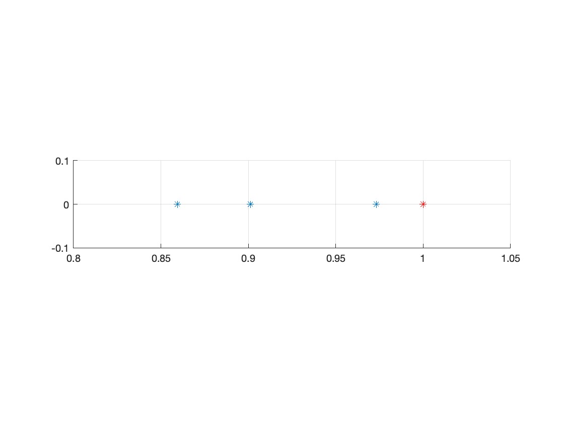
a. Allowed regions (in blue) b. Approximated eigenvalues near $1$

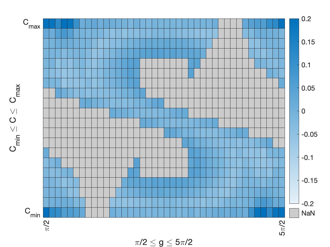
c. Eigenfunction for eigenvalue 1.00 e. Eigenfunction for eigenvalue 0.90

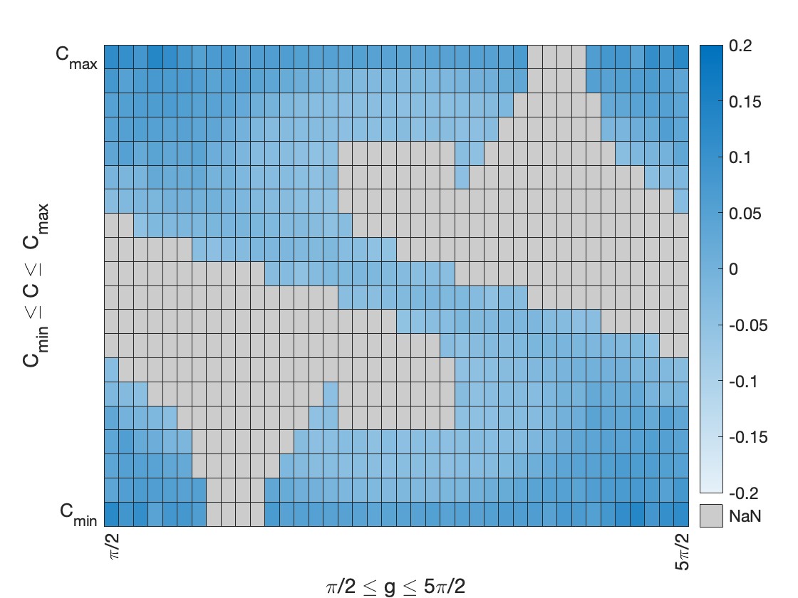
d. Eigenfunction for eigenvalue 0.97

Figure 15: Allowed regions in $(g,C)-$coordinates space $[0,2\pi)\times[C_{min},C_{max}]$. Eigenvalues and eigenfunctions of approximated Koopman operator for $\alpha=4.0,\beta=0.5,N=800,L=25$, Gauss-Legendre quadrature.

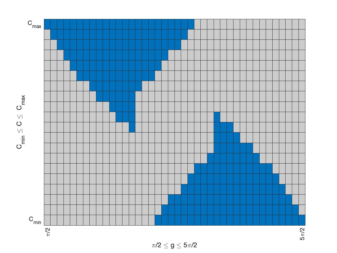
a. Allowed regions (in blue) b. Approximated eigenvalues near $1$

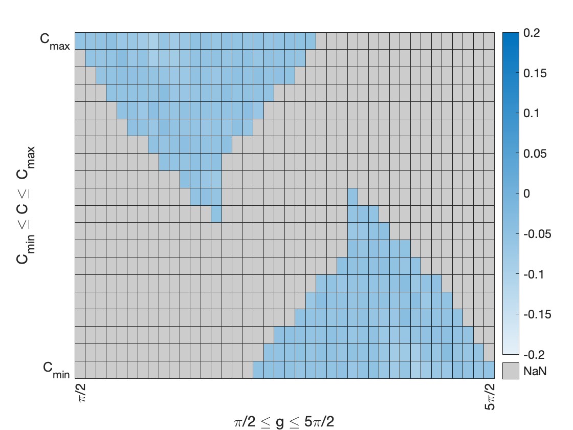
c. Eigenfunction for eigenvalue 1.00

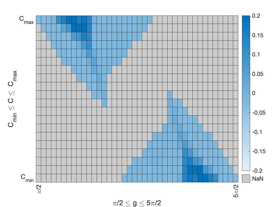
d. Eigenfunction for eigenvalue 0.91

Figure 16: Allowed regions in $(g,C)-$coordinates space $[0,2\pi)\times[C_{min},C_{max}]$. Eigenvalues and eigenfunctions of approximated Koopman operator for $\alpha=4.0,\beta=2.4,N=800,L=25$, Gauss-Legendre quadrature.

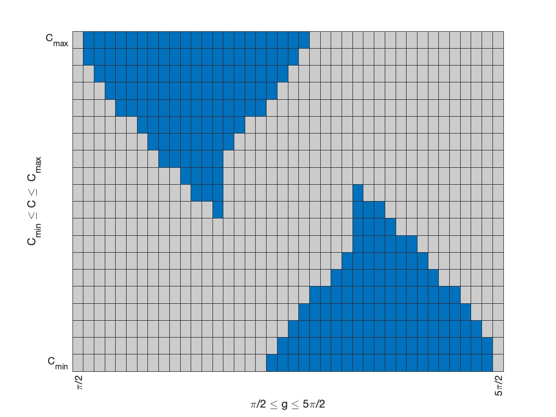
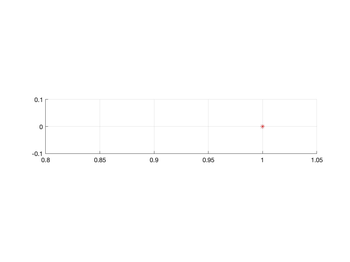
a. Allowed regions (in blue) c. Eigenfunction for eigenvalue 1.00 b. Approximated eigenvalues near $1$

Figure 17: Allowed regions in $(g,C)-$coordinates space $[0,2\pi)\times[C_{min},C_{max}]$. Eigenvalues and eigenfunctions of approximated Koopman operator for $\alpha=4.0,\beta=2.6,N=800,L=25$, Gauss-Legendre quadrature.

6.2 Discussions on the Numerical Results

The numerical results we have presented do not provide rigorous proofs, as the Galerkin approximation might not be able to capture the true eigenfunctions corresponding to eigenvalue 1 with high oscillation terms. However they suggest what the true dynamics of the corresponding systems could be.

For the Kepler case ($\beta=0$), presented in Figure 9 and Figure 14, our numerical study indicates that there is a large multiplicity for the eigenvalue 1. Also, these figures indicate that the level sets of the eigenfunctions with eigenvalue (at least close to) 1 are invariant subsets consisting of periodic trajectories. These results are compatible with the integrability of the billiard system for $\beta=0$, as it has been shown in [7].

For small values of $\beta$, our numerical results (Figure 10 and Figure 15) indicate that the there is still a large multiplicity for the eigenvalue 1 and the level sets of its eigenfunctions show many invariant subsets of the system. The system is unlikely to be ergodic. This is in consistence with the KAM stability of the integrable Boltzmann’s billiard system ($\beta=0$) under the small perturbation by the additional centrifugal force $\beta/r^{2}$ [5].

For large values of $\beta$, various types of dynamics may coexist. As one can see from the level sets of eigenfunction depicted in Figure 11 and Figure 16, for $\beta=2.4$, there exists small regions which are foliated by (quasi-)periodic trajectories and the left region is a large indecomposable invariant subset which is covered by a single chaotic trajectory. Our particular interest is the case $\beta=2.6$, presented in Figure 13 and Figure 17, in which the discretized eigenvalue problem seems to have only one simple eigenvalue in the neighborhood of 1, indicating the potential ergodicity of the system.

Acknowledgement A.T. and L.Z. are supported by DFG ZH 605/1-1, ZH 605/1-2.

Michael Plum

Karlsruhe Institute of Technology, Germany.

E-mail address: michael.plum@kit.edu

Airi Takeuchi

University of Augsburg, Augsburg, Germany.

E-mail address: airi1.takeuchi@uni-a.de

Lei Zhao

University of Augsburg, Augsburg, Germany.

E-mail address: lei.zhao@math.uni-augsburg.de

References

- [1] L. Boltzmann, Lösung eines mechanichen Problems, Wiener Berichte, 58: 1035–1044, (1868), Wissenschaftliche Abhandlungen, Vol. 1, 97–105.
- [2] S. Earnshaw, Dynamics: Or an Elementary Treatise on Motion. J. & JJ. Deighton, Cambridge, (1832).
- [3] T. Eisner, B. Farkas, M. Haase, and R. Nagel. Operator Theoretic Aspects of Ergodic Theory, volume 272. Springer, Cham, (2015).
- [4] A. Ern, and J.-L. Guermond, Theory and practice of finite elements, volume 159, Springer New York, (2004).
- [5] G. Felder, Poncelet Property and Quasi-periodicity of the Integrable Boltzmann System, Lett. Math. Phys., 111(1): 1–19, (2021).
- [6] G. Gallavotti, Nonequilibrium and Irreversibility, Springer, Berlin, (2014).
- [7] G. Gallavotti, and I. Jauslin, A Theorem on Ellipses, an Integrable System and a Theorem of Boltzmann, arXiv:2008.01955, (2020).
- [8] J.-L. Lagrange, Mécanique Analitique, Veuve Desaint, (1788)
- [9] S. M. Rump, INTLAB - INTerval LABoratory, In Tibor Csendes, editor, Developments in Reliable Computing, pages 77-104. Kluwer Academic Publishers, Dordrecht, (1999). http://www.ti3.tuhh.de/intlab.
- [10] A. Takeuchi, and L. Zhao, Conformal Transformations and Integrable Mechanical Billiards, arXiv preprint arXiv:2110.03376, (2021).
- [11] A. Takeuchi, and L. Zhao, Projective Integrable Mechanical Billiards, arXiv preprint, arXiv:2203.12938, (2022).
- [12] A. Takeuchi, Integrability and Chaotic Behavior in Mechanical Billiard Systems, Ph.D. Thesis at Karlsruhe Institute of Technology, DOI: 10.5445/IR/1000151342, (2022)
- [13] L. Zhao, Projective dynamics and an integrable Boltzmann billiard model, Comm. Contem. Math., 24(10), 2150085, (2021).