CDMPP: A Device-Model Agnostic Framework for Latency Prediction of Tensor Programs

Abstract.

Deep Neural Networks (DNNs) have shown excellent performance in a wide range of machine learning applications. Knowing the latency of running a DNN model or tensor program on a specific device is useful in various tasks, such as DNN graph- or tensor-level optimization and device selection. Considering the large space of DNN models and devices that impedes direct profiling of all combinations, recent efforts focus on building a predictor to model the performance of DNN models on different devices. However, none of the existing attempts have achieved a cost model that can accurately predict the performance of various tensor programs while supporting both training and inference accelerators. We propose CDMPP, an efficient tensor program latency prediction framework for both cross-model and cross-device prediction. We design an informative but efficient representation of tensor programs, called compact ASTs, and a pre-order-based positional encoding method, to capture the internal structure of tensor programs. We develop a domain-adaption-inspired method to learn domain-invariant representations and devise a KMeans-based sampling algorithm, for the predictor to learn from different domains (i.e., different DNN operators and devices). Our extensive experiments on a diverse range of DNN models and devices demonstrate that CDMPP significantly outperforms state-of-the-art baselines with $14.03\%$ and $10.85\%$ prediction error for cross-model and cross-device prediction, respectively, and one order of magnitude higher training efficiency. The implementation and the expanded dataset are available at https://github.com/joapolarbear/cdmpp.

1. Introduction

The adoption of Deep Neural Networks (DNNs) in various applications has boosted the fast development of AI hardware accelerators including GPUs (e.g., T4 (nvidia2018T4, ), V100 (nvidia2017V100, ) and A100 (nvidia2020A100, )), TPUs (google2016TPU, ), Huawei Ascend (huawei2018shengteng, ), Habana Goya (habana2019goya, ), and various IoT accelerators (lin2020mcunet, ; tang2017enabling, ; mohammadi2018deep, ). It is important to select proper devices (geoffrey2021habitat, ) and DNN optimization techniques (hu2022dpro, ; jia2019optimizing, ; cai2018proxylessnas, ; chen2018tvm, ; dudziak2020brp, ; kaufman2019learned, ; kaufman2021learned, ; zhang2021nn_Meter, ) to accelerate DNN training or inference under a specified time and cost budget. The execution latency of various DNN models or operators on different devices is essential for DNN optimization and device selection. For instance, to optimize a DNN model on different devices, Deep Learning (DL) compilers (chen2018tvm, ; baghdadi2021deep_tiramisu, ; adams2019learning, ) estimate or measure the performance of different tensor programs and select the best tensor programs for each computation subgraph on various devices. Another example is that automatic model-parallel training (jia2019beyond, ) requires querying the latency of each operator of a DNN on various devices when exploring ways to deploy the DNN on a heterogeneous cluster.

Due to the large space of DNN models and devices and potentially limited access to certain devices, it may not be feasible to profile all DNN models on all devices (geoffrey2021habitat, ; liu2022nnlqp, ). Many efforts have been devoted to developing cost models to estimate the performance of DNN models or operators. AutoTVM (chen2018tvm, ) and Ansor (zheng2020ansor, ) exploit XGBoost (chen2015xgboost, ) as a cost model to estimate the performance of tensor programs, which exploits an ensemble of decision trees and gradient boosting for supervised learning of the performance. The relative performance of a tensor program is predicted, i.e., the ratio of the processing throughput of the tensor program over the throughput of the tensor program with the smallest execution time, for the same computational subgraph in a given dataset. Similarly, TLP (zhai2023tlp, ) estimates the relative time of tensor programs (i.e., the speed-up over the original tensor program after some optimizations are applied) by recursively aggregating loop and computation information of each tensor program using LSTM. The relative time may not be sufficient in different use cases. Given a dataset and a cost model trained on it, if new tensor programs are introduced for each computational subgraph, the tensor program with the largest throughput for the subgraph may differ; this necessitates modifying the entire dataset to update the relative values and re-training the cost model using the entire updated dataset. Besides, it is not feasible to aggregate the relative time of subgraphs to estimate the end-to-end execution time of a DNN model.

Some other studies (e.g., NNLQP (liu2022nnlqp, )) represent the DNN model as a graph and exploit a graph neural network (GNN) to predict the performance of the graph. They cannot provide the latency of each specific operator, which is required by systems such as DL compilers. Besides, GNN-based approaches are relatively coarse-grained by taking a DNN (sub)graph as input, not flexible and efficient enough, e.g., when two DNN models only differ on several operators.

To our best knowledge, there exists no generic predictor that can accurately estimate the absolute latency of operators from various DNN models on different devices. We consider different DNN models and devices as distinct domains and name the cross-domain learning problem as a Cross-Device and Cross-Model (CDCM) prediction problem. The CDCM problem can be divided into two subproblems: (1) cross-model performance prediction (CMPP), that is, on a specific device, modeling the performance of tensor programs extracted from different DNN models and predicting the performance of unseen tensor programs; (2) cross-device performance prediction (CDPP), predicting the performance of a tensor program on a target device, based on its performance knowledge on other devices. It is challenging to develop an accurate and efficient performance model of tensor programs for CDCM.

First, how to efficiently exploit internal structure information of DNN models is the key. Previous studies have emphasized the importance of exploiting the internal structure of tensor programs for accurate performance modeling and proposed using Abstract Syntax Trees (ASTs) as representations of tensor programs to capture their internal structure (ryu2021metatune, ; baghdadi2021deep_tiramisu, ). However, it is challenging to encode ASTs as inputs of DNNs due to the extremely irregular nature of ASTs. Simple solutions, like template-based padding (ryu2021metatune, ) and AST architecture clustering (baghdadi2021deep_tiramisu, ), significantly decrease training efficiency, as they introduce significant data sparsity and small batch sizes, respectively. It is essential to efficiently process ASTs when studying the CDCM problem due to the large dataset involved (we use Tenset (zheng2021tenset, ) with over 50 million samples, each of which is a record of a tensor program and its measured execution time on a specific device).

Next, cross-model and cross-device distribution shifts are difficult to handle . Tensor programs from different DNN models and various devices can follow varying distributions of arithmetic features, memory access patterns and loop nesting, which makes it challenging to learn the universal correlations among tensor programs and their performance (kaufman2021learned, ). Separately maintaining a cost model for each device or each operator type is not a scalable solution (geoffrey2021habitat, ). Some prior studies (ryu2021metatune, ; zhao2022moses, ; liu2022nnlqp, ; zhai2023tlp, ) exploit transfer learning to adapt a cost model to a new device; they do not specify how to effectively collect traces from the target device for fine-tuning. Due to the large cost of trace collection, it is essential to sample a small set of representative tensor programs that can make the cost model adjust faster to the target device, especially with limited time and monetary budgets.

We propose CDMPP, an efficient framework to predict the absolute execution latency of tensor programs from different DNN models across various devices, including both training and inference accelerators. CDMPP introduces a regular and training-friendly structure, namely Compact ASTs, to capture the internal structure of tensor programs for efficient processing. To address the distribution shift, CDMPP learns domain-invariant representations of tensor programs by explicitly minimizing the distribution discrepancy across DNN models and devices , and proposes a clustering-based sampling strategy to guide profiling on the target device. CDMPP also utilizes a replayer to estimate end-to-end DNN performance in a bottom-up manner, with the estimated latency of each tensor program. In summary, we make the following contributions in this paper:

$\triangleright$ To exploit the internal structure of tensor programs efficiently, we introduce a concise yet training-friendly representation of tensor programs, namely Compact ASTs, and a pre-order-based position encoding method. Compact ASTs are regular with a small range of sequence lengths, which enables large-batch training without introducing data sparsity and any loss of loop information.

$\triangleright$ We perform theoretical and empirical analysis on domain differences presented in both CDPP and CMDD cases. Accordingly, we introduce a domain-shift-based regularization term into our training objective, to learn domain-invariant representations that are robust to various DNN models and devices. To avoid large trace collection overhead when adapting the cost model to a new device, we design a KMeans-based sampling algorithm to select representative samples on the target device for profiling. We also utilize a scale-insensitive training objective and the Box-Cox transformation to handle dataset skewness (wang2023margin, ) that arises from low-frequency large-cost samples.

$\triangleright$ We expand the Tenset dataset to include a broader range of devices, e.g., GPUs (e.g., A100, V100, P100) and inference accelerators (e.g., HL-100), and provide a larger dataset better suited for the CDCM problem. The expanded dataset is open-sourced to facilitate future research in this direction.

$\triangleright$ Our extensive experiments show that CDMPP achieves $14.03\%$ and $10.85\%$ prediction error for cross-model and cross-device tensor program latency prediction, respectively. In addition, the training throughput of CDMPP is one order of magnitude higher than the other DNN-based methods.

2. Background and Motivation

2.1. Deep Learning Compilers

DL compilers (chen2018tvm, ; baghdadi2021deep_tiramisu, ; adams2019learning, ; lattner2020mlir, ) have recently emerged that optimize DNN models in both the graph level and the tensor level and convert DNN models written with different ML frameworks (e.g., TensorFlow (abadi2016tensorflow, ), PyTorch (paszke2019pytorch, )) to hardware code. State-of-the-art DL compilers consist of three parts: 1) frontends that treat DL models as computational graphs and perform graph-level and tensor-level optimizations on computational graphs written in different high-level languages; 2) unified Intermediate Representations (IRs) to represent DNN models lowered from different frontends; 3) device-specific backends, each of which translates the IR to hardware code that can run on the specific device (aka code generation).

TVM (chen2018tvm, ) is a popular open-source DL compiler whose frontends decompose the high-level computational graph to a set of computational subgraphs after applying graph-level optimizations. Each subgraph corresponds to one or several operator(s) in the original DNN model. TVM performs tensor-level optimization by applying some schedule primitives on each subgraph to generate a tensor program in the form of TVM IR (TIR). With various combinations of schedule primitives, one subgraph can be converted to tens of thousands of tensor programs. TVM’s auto-tuning scheduler (zheng2020ansor, ) assigns a task for each subgraph to search for its optimal tensor program. To demonstrate the effectiveness of our proposed framework, we estimate the performance of tensor programs written as TIR on diverse devices, considering TVM’s popularity in this community. The same idea can be applied to other DL compilers.

Method	Absolute Time Prediction	Model Level Prediction	Op/kernel-level Prediction	Cross-device
AutoTVM (chen2018tvm, )(2018)	✗	✓	✓	✗
Tiramisu (baghdadi2021deep_tiramisu, )(2021)	✗	✗	✓	✗
Kaufman, et al. (kaufman2021learned, ) (2021)	✓	✓	✓	✗
MetaTune (ryu2021metatune, ) (2021)	✓	CNNs only	Conv and MatMuls only	✗
Habitat (geoffrey2021habitat, ) (2021)	✓	✓	✓	GPUs only
NNLQP (liu2022nnlqp, )(2022)	✓	✓	✗	✓
TLP (zhai2023tlp, )(2023)	✗	✓	✓	✓
CDMPP	✓	✓	✓	✓

Table 1. Prior research on DNN performance prediction.

2.2. Cross-Device Cross-Model (CDCM) Prediction

We aim to develop a generic cost model to estimate the absolute time of different tensor programs on diverse devices.

Why cross-model?  DNN optimizations, including Neural Architecture Search (NAS) (pham2018efficient, ), graph-level optimization (e.g., operator fusion (jia2019optimizing, ; jia2019taso, )) and tensor-level optimization (e.g., loop tiling (chen2018tvm, )), involve performance queries of operators from different DNN models. To handle behavior differences between different operators and distribution shifts between DNN models, one intuitive approach is to maintain a cost model for each kind of operator. Habitat (geoffrey2021habitat, ) learns an MLP for each kind of operator that uses different GPU kernels in the source and target devices, including 2D Conv2D, LSTM, etc. This approach is not scalable due to the diversity of DNN operators, especially when the operators can be fused or partitioned. It will be very useful to design a unified cost model that can predict the performance of unseen tensor programs or DNN models.

Why cross-device?  DL users often need to decide which hardware accelerators to use. For example, given a DNN model, a developer may have the following options to run model training or inference: 1) a private computer with desktop GPUs, e.g., 2080Ti(nvidia20182080Ti, ); 2) a cluster within an organization equipped with server-class GPUs (e.g., V100(nvidia2017V100, ), A100(nvidia2020A100, )); 3) CPUs (e.g., Intel Platinum(intel2019platinum, ), AMD EPYC(amd2019epyc, )) or inference accelerators such as Habana HL-100(habana2019goya, ). These options vary vastly in performance and monetary cost. Estimating the performance of DNN models on specific devices before renting or purchasing them can significantly help users make better decisions to meet their latency and monetary budgets. It is hence critical to devise a predictor that can estimate DNN Performance on various devices, including both training and inference accelerators.

Another application where both CMPP and CDPP are required is to automatically search for the optimal model parallelism strategy, i.e., determining which operators to be deployed on which devices, especially when running a DNN model on a set of heterogeneous devices. The search algorithm needs to query the latency of an operator if the operator is unseen (i.e., CMPP) or the operator is deployed on an unseen device (i.e., CDPP).

Table 1 summarizes recent studies on DNN performance prediction grouped into two categories. The first group focuses on performance modeling on a specific device, i.e., CMPP. For instance, AutoTVM (chen2018tvm, ) utilizes XGBoost (chen2015xgboost, ) to predict the relative performances of tensor programs. Tiramisu (baghdadi2021deep_tiramisu, ) designs an LSTM-based recursive cost model for performance speedup prediction on CPUs when code transformations are applied. Kaufman et al. (kaufman2021learned, ) exploit a GNN to predict the latency of a subgraph on Tensor Processing Units (TPUs). MetaTune (ryu2021metatune, ) introduces a graph template to generate uniform input features. The second group includes solutions specifically designed for CDPP. Habitat (geoffrey2021habitat, ) leverages the Roofline model (williams2009roofline, ) to scale the performance of an operator from one GPU to a different GPU but requires the operator to be implemented using the same kernels in the two GPUs. NNLQP (liu2022nnlqp, ) supports model-level latency queries on various hardware using a GNN-based feature extractor and device-specific regression layers. TLP (zhai2023tlp, ) suggests extracting features from schedule primitives for tensor programs to avoid heavy feature engineering but targets relative performance prediction. In summary, there exists no cost model that can predict the absolute time at the op- or tensor-program-level and supports both training and inference accelerators.

(a) Fused Convolution and ReLU kernel

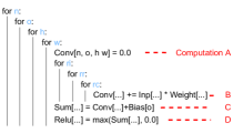
(b) Tensor programs

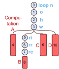
(c) Tiramisu’s AST.

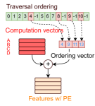
(d) Compact AST and Positional Encoding (PE)

Figure 1. Example tensor program and AST. Numbers in black are used to identify nodes.

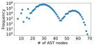
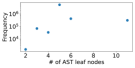
Figure 2. AST node number distribution in Tenset dataset: a) the distribution of node number in ASTs; b) distribution of leaf node number in ASTs.

2.3. Challenge in AST Feature Extraction

Selecting a proper representation of tensor programs is important for accurate performance modeling. Previous works (baghdadi2021deep_tiramisu, ; ryu2021metatune, ) have represented tensor programs as Abstract Syntax Trees (ASTs). Fig. 1 shows an example of the tensor programs of a fused Convolution and ReLU kernel (Fig. 1(b)) and its AST (Fig. 1(c)) constructed with Tiramisu (baghdadi2021deep_tiramisu, ). There are two types of nodes in the proposed AST format in Tiramisu: 1) leaf nodes, where computation and memory access happen; 2) non-leaf nodes without node features, representing loop variables. Treating each loop variable as a node in the AST results in extremely irregular AST structures (i.e., the number of nodes and their positions vary significantly across ASTs of different tensor programs), due to the complex and diverse structures of tensor programs. Fig. 2 plots the distribution of node numbers in ASTs in the Tenset dataset and the range of node numbers is large.

To exploit the internal structure of ASTs, Tiramisu (baghdadi2021deep_tiramisu, ) proposes an LSTM-based recurrent and recursive network (RNN) to iteratively aggregate an AST by traversing all nodes in the AST. However, this traversal process is highly dependent on the AST structure and only inputs with the same AST architecture can be batched together for learning. Due to irregular AST structures, batch sizes used in the training process in Tiramisu are small, resulting in low computation resource utilization and extremely low training efficiency (kosaian2021boosting, ). To extract uniform AST-based features for execution time prediction of convolutional neural networks (CNNs) at the kernel level, MetaTune (ryu2021metatune, ) augments each extracted AST to fit into a uniform super-graph template dedicated to convolution kernels. However, it is difficult to extend the template to other types of kernels due to the complexity and diversity of different kernels. Besides, given a large number of irregular AST structures, aligning small ASTs to a large template introduces significant sparsity into features, preventing efficient and accurate learning of the cost models (petrini2022learning, ).

Opportunity. Fig. 2 shows that the range of leaf node number in the ASTs is much more limited. We are inspired by this observation to design a regular feature structure by keeping only leaf nodes and incorporating loop information (e.g., the nesting level, and loop variable range) into the computation vector extracted for each leaf node. As a result, the AST is converted into a sequence of computation vectors of similar length. To ensure that the locations of leaf nodes in the AST are not lost, we record them and encode them into the sequence.

2.4. Challenge in Cross-Domain Prediction

The distribution of tensor programs in different DNN models varies due to the difference in the types of operators used. For instance, CNNs (he2016resnet, ) typically have a higher proportion of convolutional operators, while RNNs tend to be dominated by recurrent units and LSTM operators. Some previous methods (geoffrey2021habitat, ; kaufman2021learned, ) maintain a unified cross-model by assigning a unique $op\_id$ to each type of operator and combining the $op\_id$ with operator-specific parameters to generate features. However, the $op\_id$s fail to reflect the correlation between different operators, making the predictor fail to generalize to new operators. Instead, we expect a cost model that learns a common representation that can be generalized across various DNN models with different operators.

In addition, running the same set of tensor programs on different devices often leads to vastly different performances. The performance difference is hard to be estimated only using simple hardware parameters such as peak FLOPS and memory bandwidth, even when the devices are from the same hardware vendor (e.g., different models of NVIDIA GPUs) (geoffrey2021habitat, ). To address the performance shift between devices, previous works (ryu2021metatune, ; zhao2022moses, ; liu2022nnlqp, ; zhai2023tlp, ) have suggested fine-tuning the cost model on the target device. However, they do not discuss which tensor programs to profile on the target device for cost model fine-tuning, which is very relevant when the target device is not always available, and profiling the whole DNN model is very time-consuming. For example, profiling all tensor programs in the Tenset dataset on one specific device takes days and even weeks. It is important to select tensor programs that can better represent the entire dataset to profile, for achieving better fine-tuning results with limited resources.

Opportunity. TIRs provide a common representation for tensor programs of different computational subgraphs, enabling us to learn the correlations among tensor programs from different subgraphs. For cross-device learning, assuming that the same set of tensor programs are run on different devices, we can leverage the extracted features in the source devices to identify tensor programs that can best represent the entire set of tensor programs.

3. CDMPP Overview

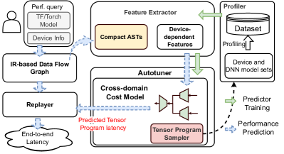
Figure 3. CDMPP Overview

3.1. Problem Formulation

We aim to build a predictor for precise performance prediction of tensor programs from different DNN models on various devices, i.e., solving the CDCM problem. Formally, the goal of the predictor is to predict the latency $\mathbf{y}$ of a tensor program using the TIR presentation $\mathbf{x}$ of the tensor program.

Intuitively, different DNN models $M$ would induce different sets of TIR presentations of tensor programs due to the different types of operators they use. We can view the TIR representation $\mathbf{x}$ from model $M$ as generated from a distribution $\mathbb{P}_{M}$, dependent on the model $M$. The performance of a tensor program would condition on the device $D$ it runs (geoffrey2021habitat, ), and we use $\mathbb{P}(\mathbf{y}|\mathbf{x},D)$ to denote the execution time distribution for $\mathbf{x}$ with a given device $D$. Our CDCM prediction problem with model $M$ and device $D$ is to learn a cost model to predict the performance of any tensor program from model $M$ on device $D$, with input $x$ generated from distribution $\mathbb{P}_{M}(\mathbf{x},\mathbf{y}|D)=\mathbb{P}_{M}(\mathbf{x})\mathbb{P}(\mathbf{y}|\mathbf{x},D)$.

Let $\mathbb{D}$ denote the set of all devices and $\mathbb{M}$ be the set of all DNN models. We use $\mathcal{F}(.)$ to represent our cost model and $\mathcal{L}(\textperiodcentered,\textperiodcentered)$ as a loss function to measure the difference between the predicted execution time and the ground truth $\mathbf{y}$. The CDCM tensor program performance prediction problem can be formulated as follows:

(1) $$\min_{\mathcal{F}}\max_{M\in\mathbb{M},D\in\mathbb{D}}\mathbb{E}_{(\mathbf{x},\mathbf{y})\sim\mathbb{P}_{M}(\mathbf{x},\mathbf{y}|D)}[\mathcal{L}(\mathcal{F}(\mathbf{x}),\mathbf{y})|D].$$

In practice, we do not have thorough access to data from all possible models $\mathbb{M}$ and devices $\mathbb{D}$. We rely on a finite dataset $\mathcal{S}$ sampled from some finite mixtures of the distributions $\mathbb{P}_{M}(\mathbf{x},\mathbf{y}|D)$ to support prediction modeling. For instance, we study the CDCM problem on the Tenset (zheng2021tenset, ) dataset, with records extracted from 120 ML models on 2 GPU models and 4 CPU models. We also supplement the dataset with 3 more GPU models and an inference accelerator. $\mathcal{S}$ is partitioned into $\mathcal{S}^{train}$, $\mathcal{S}^{valid}$ and $\mathcal{S}^{test}$, which as the prediction model training set, validation set, and test set, respectively.

We use a DNN as our prediction model. It is difficult to learn an accurate prediction model as the observations in the training data cannot cover data from all possible devices and DNN models. We are inspired by the recent research on learning an invariant representation function (stojanov2021domain, ), that allows us to effectively encode information from different devices and models into a common latent space. Representative DNN models can often be interpreted as an encoder-decoder structure, where the encoder ($h$) extract useful information from the input data into a latent representation and the decoder ($f$) maps the latent to a prediction. We thus have $\mathcal{F}=f\circ h$, where $f$ is a regression function. Domain invariant learning is to learn an encoder that gives rise to an equal conditional distribution, i.e., the statistical heterogeneity from different devices and models is mitigated in the latent representation space:

(2) $$\mathbb{P}(\mathbf{y}|h(\mathbf{x}),D,M)\approx\mathbb{P}(\mathbf{y}|h(\mathbf{x}),D^{\prime},M^{\prime}),$$

$$\forall D,D^{\prime}\in\mathbb{D},\forall M,M^{\prime}\in\mathbb{M}.$$

Such a representation $\mathbf{z}=h(\mathbf{x})$ will bring a bounded generalization risk and improve the prediction results (as detailed in Sec. 5.3).

3.2. CDMPP Architecture

We propose CDMPP, a system to tackle the CDCM problem, that efficiently learns a predictor to accurately estimate the latency of tensor programs across various DNN models and devices. Fig. 3 illustrates the architecture of CDMPP.

Feature Extractor extracts device-independent features $x$ in the form of compact ASTs from tensor programs, to capture the internal structure of the programs. A customized positional encoding method is used to aggregate the ordering vector and computation vectors of each compact AST. The Feature Extractor also extracts device-dependent features $\upsilon$, e.g., clock frequency, peak FLOPS, memory bandwidth, cache size, etc., which are used for cross-device learning.

Cross Domain Learner maintains the performance predictor $\mathcal{F}(\cdot)$. The predictor contains a Transformer-based encoder and a linear decoder. The encoder also contains multiple linear embedding layers for different compact AST architectures, each of which is responsible for generating embeddings $z_{x}$ for ASTs with the same specific number of leaf nodes. The learner is pre-trained on the training set $\mathcal{S}^{train}$. To learn from different domains (aka different DNN models and devices), we incorporate a CMD-based regularization term into the training objective, such that the distribution difference among the latent representations (i.e., the output of the encoder) of tensor programs from different DNNs and devices is minimized. Here, CMD (Central Moment Discrepancy (long2016cmd, )) is a metric for distribution difference. For cross-device learning, we train the predictor with $\mathcal{S}^{train}$ and fine-tune it with sampled features from the target device. The learner also contains an auto-tuner that performs an automatic search for optimal hyper-parameters and neural architecture for the predictor.

End-to-end Performance Prediction. To evaluate the end-to-end execution time of a DNN model, the DNN model is dissected into a set of tensor programs, and a tensor-program-based Data Flow Graph (DFG) is constructed (each node in the DFG represents a tensor program and the edges describe dependencies between tensor programs), by the DFG handler. For each tensor program, the Feature Extractor parses its features and queries the predictor to obtain its execution time. A replayer then simulates the execution of the DNN model on a specific device: it decides the execution order and timestamps of each tensor program using a topological sorting algorithm (hu2022dpro, ), based on the tensor-program-based DFG and predicted time of each tensor program, thus obtaining the end-to-end execution time.

We next detail the design of compact AST and custom positional encoding method in Sec. 4, describe the predictor architecture and cross-domain learning design in Sec. 5.

4. Feature Extraction

4.1. Compact AST

Feature engineering is a vital step in tensor program latency modeling. Device-independent factors that affect tensor program performance can be divided into three categories: 1) computation expressions, corresponding to leaf nodes in ASTs, which describe the detailed computation type and memory pattern; 2) loop information related to each computation expression, including the number of loops, lengths of loops (i.e., iteration range of loop variables) and each loop’s property (e.g., whether a loop is vectorized, unrolled or parallelized); 3) the location of each computation expression in the tensor program, which may affect memory locality. Our goal is to design an AST-based feature format that encapsulates all necessary information in a compact and regular structure so that our predictor can efficiently consume features without any loss of useful information.

We carefully design a Compact AST to represent each tensor program. Based on the AST of a tensor program (e.g., as built with Tiramisu (baghdadi2021deep_tiramisu, )), we extract a computation vector with the same set of features for each leaf node of an AST as in , which consists of computation and memory access, loop information related to each computation expression, i.e., the first two categories of device-independent factors summarized above. As illustrated in Fig. 1(d), we also serialize the original AST based on the pre-order traversal with a special maker, e.g. -1 in our case, appended after each leaf node, to capture locations of computation expressions (leaf nodes) and loop nesting information. We record the index of each leaf node in the traversal ordering and generate the ordering vector used for positional encoding. The computation vectors of leaf nodes and the ordering vector constitute a Compact AST.

Compared to original ASTs, the Compact AST design reduces the feature size while retaining all device-independent factors that may affect tensor program performance. As the range of leaf node number is small among tensor programs (Fig. 2), our feature size is more regular. We design a predictor learning framework (Sec. 5.1) based on the leaf node number, to effectively handle the variable-length feature inputs without much overhead.

4.2. Positional Encoding

We encode the computation vectors of leaf nodes and the serialized AST to generate our feature for each tensor program (Fig. 1(d)) using positional encoding (PE). Positional encoding has been commonly used in Natural Language Processing (NLP) and Computer Vision (CV) to represent the position of an element in a sequence in the input to a neural network (attention2017, ; devlin2018bert, ; dai2019transformer, ). We consider the sequence of leaf nodes (expressions) in a Compact AST and utilize the ordering vector in the Compact AST to calculate positional encoding for each leaf node, such that its position in the original AST is encoded by a unique representation. Specifically, let $N_{entry}$ be the length of the computation vector of each leaf node. Let $\mathcal{V}$ be the ordering vector, the position encoding of the $\xi$-th leaf node is computed as

$$position(\xi,2\delta)=\sin{(\frac{\mathcal{V}[\xi]}{\Theta^{2\delta/N_{entry}}})}$$

$$position(\xi,2\delta+1)=\cos{(\frac{\mathcal{V}[\xi]}{\Theta^{2\delta/N_{entry}}})}$$

where $\delta\in[0,N_{entry}/2]$ denotes the entry id in the output positional embedding, and $\Theta$ is a user-defined scalar that affects how fast frequencies are decreasing along the vector dimension and is usually set to 10000 (attention2017, ).

4.3. Device-dependent Features

The Feature Extractor extracts not only Compact ASTs but also device-dependent features. These features are related to hardware specifications of each device such as clock frequency, memory bandwidth, computation cores, the peak number of floating-point operations per second (FLOPS) in different precisions, L1/L2 cache size, memory size, etc. They are used to model how a tensor program would perform on a specific device, for cross-device performance prediction.

5. Cross-Domain Learning

5.1. Predictor Model Architecture

We adopt a Transformer-based architecture to encode feature inputs to our predictor. Recent research (attention2017, ) has proven that Transformer outperforms LSTMs  (baghdadi2021deep_tiramisu, ; steiner2021value, ) in tasks processing sequence inputs. In addition, a Transformer architecture can be parallelized for more efficient training. We do not use a GNN as GNN layers assume permutation-invariant property of the input data, which may result in loss of ordering information in the subgraphs (meltzer2019pinet, ).

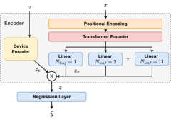
Figure 4. Predictor Model Architecture

As shown in Fig. 4, we feed the device-independent Compact AST $x$ to position encoder, then a Transformer Encoder and a leaf-node-number-specific embedding layer to generate embedding $z_{x}$ of a fixed sequence length. We also feed device-dependent features $\upsilon$ to an MLP network to compute embedding $z_{\upsilon}$. The device-dependent embedding $z_{\upsilon}$ is further aggregated with device-independent embedding $z_{x}$ to produce embedding $z=z_{x}\bigotimes z_{\upsilon}$, which is then fed into the decoder to generate the time prediction $\hat{y}$.

To address the variable-length input due to different leaf node numbers in the Compact ASTs, we use different linear layers to process outputs of the Transformer encoder according to the respective leaf node number ($N_{leaf}$), i.e., outputs corresponding to Compact ASTs of the same leaf node number are processed by the same linear layer. The linear layers produce embedding $z_{x}$ of the same length. Compared to the common padding approach that adds zero paddings to force uniform input sequences (ryu2021metatune, ), this leaf node number-based method guarantees uniform input shapes to the decoder without introducing additional sparsity and computation, leading to more efficient predictor model learning. Given the limited range of leaf node numbers, the memory overhead of keeping multiple linear layers is limited.

5.2. Pre-training with Scale-insensitive Training Objective

A machine learning-based cost model is often trained to minimize the mean square error (MSE) (ryu2021metatune, ). However, when the range of prediction values (i.e., tensor program latencies in our case) differs substantially, MSE often leads to a model whose predictions are about the mean of the performance distribution, underestimating high-latencies and over-estimating low-latencies. Mean Absolute Percentage Error (MAPE) measures the relative error (i.e., the average absolute percentage difference between predicted values and actual values). When minimizing MAPE as the training objective, overestimation poses a risk of significantly large MAPE error ($>>1$), whereas underestimation ensures that the MAPE error remains $\leq 1$. In datasets with significant skewness, where a large portion of samples have small values, the cost model tends to produce small predicted values to prevent overestimation for samples with small actual values and achieve a low MAPE error. However, this results in large absolute errors for samples with large actual values. To balance between the absolute and relative errors, we use a scale-insensitive hybrid training objective, which minimizes MSE and MAPE concurrently. Specifically, the loss function adopted in our prediction model pre-training (on the training set $\mathcal{S}^{train}$) is as follows:

(3) $$\mathcal{L}_{pre\_train}= \frac{1}{|\mathcal{S}^{train}|}\times\left(\sum_{i\in\mathcal{S}^{train}}(\hat{\mathbf{y}}_{i}-\mathbf{y}_{i})^{2}+\right.$$

$$\left.\lambda\sum_{i\in\mathcal{S}^{train}}|\hat{\mathbf{y}}_{i}-\mathbf{y}_{i}|/\mathbf{y}_{i}\right)$$

where $\lambda$ is a coefficient to ensure the same order of magnitude of MSE and MAPE terms. We empirically find $\lambda=10^{-3}$ performs well in our experiments.

5.3. Fine-tuning with CMD-based Regularization

For better prediction performance on a target domain, we fine-tune the prediction model with ${\mathcal{S}^{train}}$ and only the input features in the target domain. Fine-tuning aims to minimize both the hybrid errors and the distribution difference between the latent representations (output of the encoder) from source domains and the target domain.

CMD to measure distribution difference. Our goal is for our fine-tuned predictor to perform well on different DNN models and devices. One of the most important theoretical results in domain invariant learning is that the generalization risk of the model (i.e., the difference in the average error of a cost model evaluated on model $M$ and device $D$ versus that on model $M^{\prime}$ and device $D^{\prime}$) can be mitigated by reducing the distance among different domains in the latent space (redko2020survey, ). To put this in our context, recall that $h$ is our encoder that maps input features to the latent space. With a suitable distribution difference metric $\Delta(\cdot)$, we have the following bound on the generalization risk for $D,D^{\prime}\sim\mathbb{D}$ and $M,M^{\prime}\sim\mathbb{M}$ (redko2020survey, ):

(4) $$\mathbb{E}_{(\mathbf{x},\mathbf{y})\sim\mathbb{P}_{M}(\mathbf{x},\mathbf{y}|D)}[\mathcal{L}(\mathcal{F}(\mathbf{x}),\mathbf{y})|D]$$

$$\leq\mathbb{E}_{(\mathbf{x},\mathbf{y})\sim\mathbb{P}_{M^{\prime}}(\mathbf{x},\mathbf{y}|D^{\prime})}[\mathcal{L}(\mathcal{F}(\mathbf{x}),\mathbf{y})|D^{\prime}]$$

$$+\Delta(\mathbb{P}(h(\mathbf{x})|D,M),\mathbb{P}(h(\mathbf{x})|D^{\prime},M^{\prime}))$$

which says the difference in the expected performance of the system between any pair of $\mathbb{P}_{M^{\prime}}(\mathbf{x},\mathbf{y}|D)$ and $\mathbb{P}_{M}(\mathbf{x},\mathbf{y}|D)$ is bounded by the distance between their induced representation distributions in the latent space.

Based on this distribution-difference-based bound, we can minimize the following objective in our model fine-tuning  (abhinav2020domain, ), to project representations of samples from different domains close together in the representation space:

(5) $$\min_{h,f} \underbrace{\quad\mathcal{L}_{pre\_train}(f(h(\mathcal{S})))}_{\text{standard training loss}}+$$

$$\underbrace{\mathbb{E}_{D,D^{\prime}\sim\mathbb{D}||M,M^{\prime}\sim\mathbb{M}}[\Delta(\mathbb{P}(h(\mathbf{x})|D,M),\mathbb{P}(h(\mathbf{x})|D^{\prime},M^{\prime}))]}_{\text{regularization for minimizing representation difference}}$$

One practical divergence measure for $\Delta(.)$ is the Central Moment Discrepancy (zellinger2019cmd, ), which is theoretically grounded, efficient to implement and compute, and has shown superior empirical success in learning domain invariant representations (long2016cmd, ; qi2021gnncmd, ). Given two distributions $\mathbb{P}_{1},\mathbb{P}_{2}$, the CMD distance can be defined as:

(6) $$\text{CMD}(\mathbb{P}_{1},\mathbb{P}_{2})=\frac{1}{|b-a|}\|\mathbb{E}(\mathbb{P}_{1})-\mathbb{E}(\mathbb{P}_{2})\|_{2}+$$

$$\sum_{j=2}^{\infty}\frac{1}{|b-a|^{j}}\|\Omega_{j}(\mathbb{P}_{1})-\Omega_{j}(\mathbb{P}_{2})\|_{2}$$

where $a,b$ are the joint distribution support of the distributions $\mathbb{P}_{1}$ and $\mathbb{P}_{2}$, respectively, and $\Omega_{j}(\mathbb{P}_{1})=\mathbb{E}(\mathbb{P}_{1}-\mathbb{E}(\mathbb{P}_{1}))^{j}$ is the $j$-th order moment. In practice, a limited number of moments are usually needed (e.g., $j\leq 5$) (long2016cmd, ).

We then obtain the training objective for our predictor fine-tuning as follows:

(7) $$\mathcal{L}_{fine\_tune}=\mathcal{L}_{pre\_train}+\alpha\times\text{CMD}(z_{s},z_{t})$$

where $z_{s}$ and $z_{t}$ are latent representations of the source domain (e.g., a set of devices for CDPP) and the target domain (e.g., a set of devices disjoint to source devices for CDPP), respectively. $\alpha$ is a coefficient decided by the auto-tuner.

Sampling Strategy for Fine-tuning on Target Device. To achieve fast fine-tuning for accurate performance prediction on a new device, we should select tensor programs that best represent the entire dataset to profile on the target device. As tensor programs for different devices may not be exactly the same (e.g., a tensor program for GPU cannot be directly run on CPU), we sample representative tasks (instead of tensor programs) and profile the respective tensor programs of the tasks on the target device. We consider the same set of $\mathbb{T}$ tasks on different devices. Each task $\tau$ in set $\mathbb{T}$ has a set of device-independent features $X_{\tau}$ (including features of its tensor programs) and corresponding latent representations of its tensor programs $Z_{\tau}$. Let $Z=\bigcup_{\tau=1}^{|\mathbb{T}|}Z_{\tau}$ denote the set of all latent representations of tasks in $\mathbb{T}$. Our goal is to decide a subset $\mathcal{Q}$ of $\kappa$ tasks to profile on the target device, such that the distribution difference between the latent representations of the selected tasks and those of all tasks is minimized.

Recall that $X$ is the feature space of all possible tensor programs and $\mathcal{H}$ is the latent/embedding space. Let $\mathcal{C}=\bigcup_{j=1}^{\kappa}X_{\mathcal{Q}_{j}}$ denote the feature set of tasks used for fine-tuning. Let $c_{x}=\operatorname*{arg\,min}_{c\in\mathcal{C}}\Delta_{\mathcal{H}}(h(x),h(c))$ denote the closest $c\in\mathcal{C}$ to $x$ in the latent space, and $\epsilon:=\max_{x\in X}\min_{c\in\mathcal{C}}\Delta_{\mathcal{H}}(h(x),h(c))$, which captures the maximal distance between any tensor program in the input space and the closest tensor program among the finetuning samples in the latent space. We derive the following bound for the generalization risk of the fine-tuned model with respect to the sampling strategy (see Appendix A for the detailed proof):

(8) $$\mathcal{L}_{\mathrm{pre\_train}}(x)\leq\mathcal{L}_{\mathrm{pre\_train}}(c_{x})+\mathcal{O}(\epsilon)$$

We propose a clustering-based sampling strategy that minimizes $\epsilon$ and hence lowers the generation risk, as shown in Algorighm 1. We first perform K-means clustering to divide all tensor program features in $X$ into $\kappa$ clusters, $\mathbb{G}_{e},e=1,2,...,\kappa$, which are sorted according to the cluster size (line 1-2). Then we calculate a table $\Psi$, with entry $\Psi[e,\tau]=(\sum_{j=1}^{|X_{\tau}|}||\mathbb{G}_{e}-X_{\tau}[j]||_{2})/|X_{\tau}|$ denoting the average distance of task $\tau$’s features $X_{\tau}$ to the center of cluster $e$ (line 6). We pick one task for each cluster to profile starting from the cluster with the largest cluster size and remove the task from the candidate task set once it is selected. Specifically, for cluster $e,e=1,2,...,\kappa$, we select the task with the smallest $\Psi[e,\tau]$ value in the candidate set (line 9-15).

Algorithm 1 Clustering-based sampling strategy

1:all tensor program features $X$, number of tasks to select $\kappa$, all tasks $\mathbb{T}$

2:Selected tasks $\mathbb{T}^{*}$

3:$\mathbb{G}\leftarrow\textsc{KMeans}(X,\kappa)$

4:Sort $\mathbb{G}$ in descending order according to the cluster size

5:$\mathbb{T}^{*}\leftarrow\emptyset$

6:for $e=1\rightarrow\kappa$ do

7:    for $\tau=1\rightarrow|\mathbb{T}|$ do

8:         $\Psi[e,\tau]=(\sum_{j=1}^{|X_{\tau}|}||\mathbb{G}_{e}-X_{\tau}[j]||_{2})/|X_{\tau}|$

9:    end for

10:    $d\leftarrow$ sorted index of $\Psi[e,1:|\mathbb{T}|]$ in ascending order

11:    for $\tau$ in $d$ do

12:         if $\tau$ in $\mathbb{T}$ then

13:             $\mathbb{T}^{*}\leftarrow\mathbb{T}^{*}\cup\{\tau\}$;$\mathbb{T}\leftarrow\mathbb{T}$\$\tau$; break

14:         end if

15:    end for

16:end for

17:return $\mathbb{T}^{*}$

NAS and Automatic hyper-parameter tuning. We employ an auto-tuner to automatically optimize the model architecture and hyper-parameters in our cost model to minimize the prediction error. For model architecture, our focus is primarily on determining the values for the number of transformer encoder layers, the number of MLP layers in the decoder, and the intermediate dimension. As for the hyper-parameters in the cost model, we conduct a search for variables such as $\alpha$ in Eqn. 7, learning rate, weight decay, optimizer (Adam or SGD), learning rate scheduler, and batch size. To implement the auto-tuner, we utilize Optuna (optuna_2019, ), a hyper-parameter optimization framework equipped with state-of-the-art exploring algorithms. We use Optuna to explore the optimal combinations of the aforementioned variables to minimize the evaluation error. Since NAS (Neural Architecture Search) and hyper-parameter search are not the primary focus of this paper, instead of exhaustively searching for the optimal combination, we terminate the auto-tuner after testing approximately 1000 configurations and choose the best one among them, which we find performs well across all our experiments. For detailed values of variables mentioned above, please refer to Appendix B.

Taxonomy	Device	Clock (MHz)	Mem. (GB)	Mem. band- width(Gbps)	Cores	$\#$ of Samples
NVIDIA GPUs	T4 (nvidia2018T4, )	1590	16	320	40	9M
	K80 (nvidia2014K80, )	824	12	240.6	26	9M
	P100 (nvidia2016P100, )	1329	16	732.2	56	9M
	V100 (nvidia2017V100, )	1530	32	900	80	2M
	A100 (nvidia2020A100, )	1410	40	1555	108	2M
Inference Accelerators	HL-100 (habana2019goya, )	1575	8	40	11	4K
CPUs	Intel E5-2673 (intel2016e5, )	2300	2048	572.24	8	9M
	AMD EPYC 7452 (amd2019epyc, )	2350	2048	1525.6	4	9M
	ARM Graviton2 (amazon2010graviton, )	2500	32	4.75	32	9M

Table 2. GPU and non-GPU devices used in evaluation

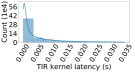
(a) Original Y

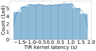
(b) Y with Box-Cox Transformation

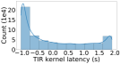
(c) Y with Yeo-Johnson Transformation

(d) Y with Quantile Transformation

Figure 5. The distribution of tensor program latency (Y) under various normalization methods. The blue line represents the kernel density estimate to smooth the distribution.

5.4. Handling Dataset Skewness

Most ML algorithms exhibit better performance when the input features and output predictions follow standard distributions such as a Gaussian (normal) distribution or the uniform distribution  (dasgupta2011probability, ). The dataset we use, which contains Tenset and our own profiled records, is generated by randomly sampling schedules for tasks in various DNN models and collecting their performance on different devices. Fig. 5(a) exhibits a long tail distribution of tensor program latencies in the dataset. Such skewness may significantly hinder an accurate prediction model (hsieh2020non, ).

Power transformation (weisberg2001yeo, ) is a technique to map a non-normal probability distribution more Gaussian-like, which can be used to alleviate the effect of outliers. One example of a power transformation is the Box–Cox transformation (box1964analysis, ), which fits an optimal parameter for the mapping through maximum likelihood estimation. Another example is Yeo-Johnson transformation, which can handle negative values and zeros. Quantile transformation transforms variables to a standard distribution, including uniform and normal distributions, and is non-parametric.

We choose among the representative normalization methods to make our tensor program latency data more standard, by evaluating the distribution of tensor program latency after applying each method. Fig. 5 shows that the Box-Cox transformation generates a more normal and symmetric distribution with fewer outliers. Therefore, to rectify the effect of data skewness on our prediction model, we estimate the optimal parameter of the Box–Cox transformation based on the training dataset using an out-of-the-box library (sklearn_api, ) and apply inverse Box-Cox transformation to convert the latency back to the original space for error measurement.

5.5. End-to-end Performance Prediction

We have developed a replayer that leverages our cost model as a backbone to predict the end-to-end latency of a DNN model. To achieve this, we begin by constructing a TIR-based Data Flow Graph (DFG) for the given DNN model. The DFG is created by establishing connections between dependent TIR functions based on their dependencies. For each node in the DFG, we extract the corresponding TIR kernel or TIR tensor program for feature extraction. Subsequently, we utilize our cost model to estimate the latency of each node on a specific device. It is important to note that multiple TIR functions may be implemented using the same TIR kernel. In such cases, we only perform the cost model inference once for these TIR functions, optimizing computational efficiency. The replayer takes the TIR-based DFG and the execution time of each node as inputs. It decides the execution order of nodes on specific devices using a topological sorting algorithm, following the methodology outlined in (hu2022dpro, ), and takes the end time of the last scheduled node as the estimated iteration time. Please refer to Appendix C for the detailed simulation algorithm. The replay process to simulate the execution of a DFG also takes device-specific characteristics into consideration. For example, Habana HL-100 chips contain 3 GEMM cores for GEMM and convolution operations, and 8 Tensor Processor Cores (TPC) for SIMD vector computation. Taking a convolution operator with an estimated execution time of $\hat{y}$ for instance, we replace the corresponding node in DFG with 3 sub-operators that can run in parallel and each sub-operator’s execution time is $\hat{y}/3$.

6. Implementation

We extract device-independent features from TIRs using TVM v0.9.dev0 and build our prediction model using PyTorch (paszke2017automatic, ) v1.11.0+cu102. The CDMPP framework is implemented using Python with 15,331 LoC. Users can call the command as follows to query the latency of a network:

⬇

$ cdmpp <network> <batch_size> <device>

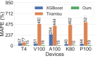
(a) GPUs

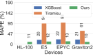
(b) Inference accelerators and CPUs

Figure 6. Comparison of prediction errors at the TIR level. The number on top of each bar is the exact MAPE value.

7. Evaluation

7.1. Experimental Setup

Testbed. We profile the ground truth of DNN models and tensor programs on devices listed in Table 2, including both GPU and non-GPU devices. To train and test the predictor and baselines, we use devices equipped with NVIDIA Tesla V100 32GB GPUs. We use CUDA v11.0 (cuda, ) and cuDNN v7.6.5 (cudnn, ) in our experiments.

Dataset. We train our cost model on a large multi-platform dataset (combining Tenset and our own profiling results), which includes tensor program performance records for 120 DL models (ResNet50  (he2016resnet, ), VGG16 (simonyan2014very, ), BERT Base (devlin2018bert, ), etc.) on 5 GPU models (Nvidia K80, P100, T4, V100, A100), three CPU models (Intel E5-2673 (intel2016e5, ), AMD EPYC 7452 (amd2019epyc, ), Graviton2 (amazon2010graviton, )), and one inference accelerator (Habana HL-100). Table 2 gives the detailed device features we use for cross-device learning and the dataset size collected from each device. For T4, K80 and CPUs, we use the data from Tenset (zheng2021tenset, ); for the remaining devices, we profile tensor program performance on them. We will release the dataset to the community. For cross-model learning, we use a test set $\mathcal{S}_{hold}$ of 3 DNN models (ResNet-50, MobileNet-V2, and BERT-tiny) for each device. We randomly split the remaining dataset into training, validation, and test sets ($\mathcal{S}^{train}$, $\mathcal{S}^{valid}$, and $\mathcal{S}^{test}$) at a ratio of 8:1:1 for pre-training. For cross-device learning, we pre-train the cost model on $\mathcal{S}^{train}$ from source devices and sample tensor programs from $\mathcal{S}^{train}$ of the target device for fine-tuning and then evaluate the predictor on $\mathcal{S}^{test}$ of the target device. We repeat each experiment 3 times and obtain the average results.

Baselines. For cross-model learning, we compare CDMPP with two SOTA predictors: XGBoost (chen2015xgboost, ), a representative rule-based ML method, and Tiramisu, which also utilizes AST-based features. We modify Tiramisu (https://github.com/ Tiramisu-Compiler/tiramisu) to enable it to support TVM and use the default settings in Tiramisu, e.g., taking MAPE as the learning objective, using cycle learning rate scheduler, etc. For cross-device learning, we use Habitat and TLP as baselines.

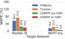
(a) Cross-model learning on T4

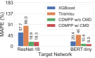
(b) Cross-model learning on EPYC

Figure 7. Comparison of cross-model prediction errors. The number on top of each bar is the exact MAPE value.

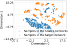
(a) w/o CMD

(b) w/ CMD

Figure 8. Hidden representation comparison when taking BERT-tiny as the target network.

7.2. Cross-Model Performance Prediction

Pre-training performance. Fig. 6 compares the prediction error of our pre-trained predictor with baselines at the TIR level on different devices. Our predictor achieves a prediction error $<16\%$ on most devices and outperforms the baselines across all devices. Tiramisu (baghdadi2021deep_tiramisu, ) exhibits large errors significantly larger than the values ($16\%$) claimed in their paper. The reason is as follows: 1) the recursive LSTM in Tiramisu requires samples in a batch to have the same original AST structure, while the structure of ASTs in our dataset is extremely irregular, as shown in Fig. 2, resulting in small batch sizes and large gradient randomness; 2) Tiramisu is primarily designed to estimate the performance speedup when some transformations are applied to a program thus may not perform optimally when estimating the absolute value of tensor programs in our dataset that encompass values across a large range; 3) As stated in their paper, Tiramisu exhibits an exponential increase in prediction error for speedups that deviate far from 1. In detail, the error is larger than $40\%$ when the speedup is smaller than 0.1, while our dataset encompasses a wide range of values, spanning from hundreds of microseconds to tens of milliseconds. This further reinforces the conclusion that Tiramisu’s performance is compromised when working with our skewed dataset that contains values across a wide range. In terms of training efficiency, our measurements of average throughput over all devices for the three methods reveal that CDMPP (14241 samples/s) improves the training throughput by 1 order of magnitude over Tiramisu (1870 samples/s), because Tiramisu’s LSTM requires recursive computation of loop embeddings according to the structure of input ASTs, with multiple forward passes through the LSTM layers in each iteration. Our predictor utilizes a simpler, more regular feature structure that enables large-batch training. The training throughput with XGBoost (644588 samples/s) is larger than ours because it ensembles simple decision trees and has a smaller prediction model size. The end-to-end training cost for the CDMPP is 1 2 hours on V100, much smaller than Tiramisu’s 9 hours.

(a) Predicted onto ResNet50, BS=1

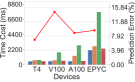
(b) Predicted onto BERT Base, BS=1

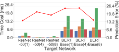
(c) End-to-end performance prediction on HL-100. ResNet-50 (1) denotes ResNet-50 with batch size=1.

Figure 9. End-to-end performance prediction for cross-model learning.

Cross-model prediction performance. We then evaluate the generalizability of our cost model to unseen DNN models by fine-tuning it with input features sampled from $S_{hold}$ for each of the three target networks. Fig. 7 plots the cross-model learning results on T4 and EPYC, which show that CDMPP always achieves the lowest prediction error. We further explore why CDMPP performs best by analyzing the hidden representations of source networks and that of the target network in Fig. 8, where t-SNE (belkina2019automated, ) is applied to reduce the representation dimension. The results show that our CMD-based regularization reduces the distribution discrepancy between latent representations from different networks and allows the predictor to generalize better to the target network.

End-to-end performance prediction. We break each DNN model down into a set of tasks and randomly sample a schedule for each task. Fig. 9 compare prediction error of end-to-end model performance against the actual measurements on corresponding devices. CDMPP incurs an average prediction error of $12.4\%$, substantially outperforming XGBoost and Tiramisu, whose average error rates are $63.8\%$ and $293.6\%$, respectively. Fig. 9(c) further demonstrate that CDMPP can accurately model the performance of HL-100.

7.3. Cross-Device Performance Prediction

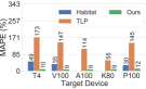
(a) Prediction onto GPU

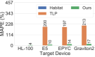
(b) Prediction onto non-GPU device

Figure 10. Comparison of cross-device prediction errors at the TIR level. The number on top of each bar is the exact MAPE value.

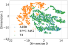
(a) Before finetuning

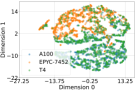
(b) After finetuning

Figure 11. Hidden representation comparison before and after fine-tuning for CDPP. Target device: EPYC.

We evaluate the cross-device prediction performance under 3 different combinations of source and target devices: 1) one GPU as target device and the remaining GPUs as source devices (from GPUs to a GPU); 2) one CPU as the target device and the remaining GPUs and CPUs as source devices (from GPUs and CPUs to a CPU; 3) the inference accelerator as the target device and all GPUs as source devices (from GPUs to the inference accelerator). Fig. 10 shows that our fine-tuning-based method achieves the lowest prediction error, $10.85\%$ on average. TLP exhibits a large prediction error on absolute time prediction (it focuses on relative time prediction). Habitat uses simple MLPs to predict the performance of the most “important” operators (conv2d, lstm, bmm and linear) with operator-level features, while in our case, one operator with a specific shape may have different tensor programs when different scheduling is applied. Habitat’s MLP-based cost model struggles to differentiate between these distinct tensor programs lowered from the same operators and has limited generalization to different operator types. In contrast, we exploit the internal structure of tensor programs to boost the learning of common representations across different tensor programs derived from different operators. Fig. 10(b) exhibits that our predictor can generalize well from GPU devices to non-GPU devices. We do not have the results of Habitat here as it only supports GPU devices. Taking the prediction experiment onto EPYC for instance, Fig. 11 shows the latent representation of different devices before and after finetuning, where t-SNE is also applied. The results indicate that our method effectively reduces the distribution shift between two GPUs, as well as between GPUs and CPUs.

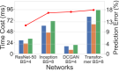
(a) Prediction onto P100

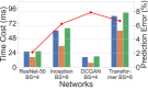
(b) Prediction onto V100

Figure 12. Cross-device end-to-end performance prediction.

We further compare cross-device end-to-end model performance prediction among CDMPP, the ground truth and Habitat in Fig. 12. Here we do not compare with TLP, since it predicts relative performance of each tensor program which cannot be accumulated as the end-to-end performance. Our method, CDMPP, consistently outperforms Habitat with smaller prediction errors in all cases. On average, the prediction error of CDMPP is $15.72\%$, and $28.01\%$ with Habitat.

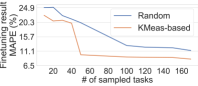
Figure 13. Effect of sampling strategy for CDPP.

Device	Box-Cox	Yeo-Johnson	Quantile	original Y
T4	15.18	49.30	17.88	72.55
A100	17.53	20.09	17.38	68.77
K80	14.79	24.88	15.37	71.34

Table 3. MAPE ($\%$) with different normalization methods.

7.4. Effect of sampling strategy in fine-tuning

We compare our KMeans-based sampling strategy to random sampling when fine-tuning the cost model (trained on all other GPUs) on T4. We repeat each experiment with random sampling 10 times and report the average results. Fig. 13 shows that when the number of fine-tuning tasks is the same, our sampling method leads to smaller prediction errors, indicating that our KMeans-based sampling strategy can find tasks that better represent the dataset. The error does not decrease as we increase the number of sampled tasks beyond 50. 50 sampled tasks contain around 100k tensor programs , which is much smaller than the size of the fine-tuning dataset used in TLP (500K).

7.5. Ablation Study

Normalization method. Table 3 compares performance of the pre-trained cost model for cross-model learning when different normalization methods are applied to the target labels. We perform the experiment on 3 devices. Box-Cox transformation leads to the smallest test errors, by making the obviously skewed data distribution in our dataset more normal. Without any normalization, the predictor tends to output a value around the mean cost for any inputs, leading to large prediction errors.

Device	MSE	MAPE	MSPE	MSE+MAPE
T4	20.69	30.74	49.47	15.18
A100	20.47	25.15	49.44	17.53
K80	17.63	28.96	212.81	14.79

Table 4. MAPE ($\%$) with different loss functions

Scale-insensitive loss function. We then evaluate the effect of different loss functions by running cross-model learning tasks on different devices. We measure both MAPE (Table 4) and RMSE (Table 5). MSPE (Mean Square Percentage Error) also measures the relative error by summing up the square of the relative error. We empirically observe that 1) taking MSE as the objective function tends to produce values close to the mean of the real values, leading to a large relative error (MAPE) for samples far away from the mean; 2) taking MAPE and MSPE as the objective function makes the predictor prefer relatively small predictions since under-estimating large values will not incur significantly large error as over-estimating small values (larger than $100\%$). In contrast, as shown in Table. 4 and Table. 5, the scale-insensitive loss function, which explicitly optimizes the absolute and relative error, outperforms any other methods in terms of both MAPE and RMSE.

Positional encoding. Fig. 14 compares the prediction errors with and without our customized positional encoding for feature generation. The results prove that positional encoding can reduce the prediction error, revealing that encoding location information of leaf nodes can indeed help the predictor capture the relationship between tensor programs and their performance better.

Schedule search. We also integrate our cost model into the auto-tuning framework in Ansor to evaluate whether it can identify better schedules. We tune a DNN network , BERT-tiny, for 2000 search rounds, and the cost model is used to prune the search space in each search round. Fig. 14 shows that using our cost model can help find better schedules. CDMPP’s inference time on V100 is  8 ms across batch sizes from 1 to 400, higher than XGBoost’s 0.2 ms. However, our schedule search experiment reveals that CDMPP can find better schedules while the time ratio for completing 2000 search rounds between CDMPP and XGB varies from 1.5:1 to 2:1. This smaller gap is primarily because Ansor’s algorithm requires performance measuring of selected candidates (e.g., 10 candidates per search round) on real devices, which incurs significant overhead, alleviating the impact of cost model latency.

Device	MSE	MAPE	MSPE	MSE+MAPE
T4	0.31	0.48	0.62	0.34
A100	0.30	0.40	0.41	0.27
K80	0.87	0.89	1.5	0.59

Table 5. RMSE ($ms$) with different loss functions

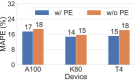
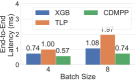
Figure 14. (a) MAPE ($\%$) w/ and w/o PE; (b) Schedule search results with different cost models for BERT-tiny on T4.

7.6. Discussion

Extend CDMPP to different DNN models. CDMPP is capable of accurately predicting the latency of various DNN models. When presented with a new DNN model, we employ a feature extraction process from its corresponding tensor programs and leverage the pre-trained cost model, which has been trained on datasets collected from multiple DNN models, for performance prediction. To enhance the generalization capability to new DNN models, we employ a cross-model fine-tuning method, as depicted in Equation  7, by taking advantage of the dataset distribution specific to the target DNN model. This fine-tuning process aids in achieving enhanced generalization and adaptability when dealing with previously unseen DNN models.

Extend CDMPP to more devices. CDMPP is not limited to cross-GPUs only. Given a cost model pre-trained on the GPU dataset, our fine-tuning approach will utilize the clustering results on the available dataset to guide trace collection on target devices, including non-GPU architectures, and adapt the cost model to the new device fast in 10-20 minutes. It never requires re-training from scratch. Fig. 10(b) shows examples of prediction from GPUs to Habana HL-100 and CPUs of different brands (e.g., Intel, ARM, AMD).

8. Related Work

Cross-device Performance Prediction.  Habitat (geoffrey2021habitat, ) proposes a roofline-model-based (williams2009roofline, ) scaling method and MLP-based model to predict performance of ops across different GPUs. TLP (zhai2023tlp, ) extracts features from schedule primitives, instead of tensor programs, and maintains a prediction head for each device. nn-Meter (zhang2021nn_Meter, ) builds a kernel-level latency predictor for model inference on diverse edge devices, but only focuses on CNNs. NNLQP (liu2022nnlqp, ) estimates the iteration time of DNN models with a device-independent GNN-based encoder and device-specific prediction heads.

Cross-model Performance Prediction.  Many works (chen2018learning, ; chen2018tvm, ; zheng2020ansor, ) maintain a cost model for each kind of DNN op (Conv2d, Matmul, etc.) or kernel (a subgraph of DNN) separately, which is not scalable considering the variety of DNN models and tensor programs. AutoTVM (chen2018tvm, ) and Ansor (zheng2020ansor, ) exploit transfer learning to avoid training cost models for each kernel from scratch, while the fine-tuning process for each kernel is still time-consuming. Besides, they only predict the relative order among optimization candidates and do not provide accurate cost estimation. Kaufman et al. (kaufman2021learned, ) decompose a DNN model into computation subgraphs and use a GNN to predict the performance of each subgraph on TPUs (you2019fast_tpu, ). Steiner et al. (steiner2021value, ) predict performance of a partial schedule using an LSTM. MetaTune (ryu2021metatune, ) and Tiramisu (baghdadi2021deep_tiramisu, ) propose AST-based representations of tensor programs to exploit the internal structure of tensor programs. We did not compare with MetaTune since it is not open-sourced.

ML Benchmarking. Benchmark results (mattson2020mlperf, ; reddi2020mlperf, ; zhu2018benchmarking, ; cuda2020benchmarking, ) are available for some specific DNN models (e.g., ResNet50 (he2016resnet, ), BERT (devlin2018bert, )) and common GPUs. Some non-GPU vendors may publish their benchmark results (mlperf, ), but are also limited to some common DNN models. We propose a system to predict the performance of any given DNN model without extensively running it on a target device, as long as the model can be represented as TIRs.

9. Conclusion

This paper presents CDMPP, an efficient framework for accurately predicting the performance of tensor programs across different DNN models and devices. The main design highlights include 1) Compact ASTs as a concise feature format to capture internal structures of tensor programs; 2) a customized positional encoding method and a Transformer-based cost model that enables efficient learning of AST-based inputs; 3) a CMD-regularization boosted training objective to learn domain-invariant representations robust to various DNN models; 4) a KMeans-based sampling strategy for cross-device fine-tuning. Our extensive experimental results demonstrate that CDMPP outperforms SOTA baselines in terms of prediction error and training throughput for both cross-model and cross-device performance prediction.

Appendix A Appendix: Proof of Eq. 8

In this appendix, we provide proof of Eq. 8, namely,

(9) $$\mathcal{L}_{\mathrm{pre\_train}}(x)\leq\mathcal{L}_{\mathrm{pre\_train}}(c_{x})+\mathcal{O}(\epsilon).$$

Proof.

First, recall that $X$ is the feature space of all possible tensor programs and $x\in X$ is a given tensor program. $\mathcal{H}$ is the latent/embedding space, and we denote $h(x)$ as the latent representation of tensor $x$ in the latent space. $C$ is our selected tensor program sample for fine-tuning.

For the analysis, we make the standard assumption that the loss function $\mathcal{L}_{\mathrm{pre\_train}}$ is $L_{k}$-Lipschitz continuous with respect to the representation in the latent space, namely, we have that

$$\|\mathcal{L}_{\mathrm{pre\_train}}(h(x))-\mathcal{L}_{\mathrm{pre\_train}}(h(x^{\prime}))\|\leq L_{k}\Delta(h(x),h(x^{\prime})).$$

Next, recall that $c_{x}=\operatorname*{arg\,min}_{c\in C}d_{\mathcal{H}}(h(x),h(c))$ is the closest $c\in C$ to $x$ in the latent space. Let’s consider the difference between $x$ and $c_{x}$. First, note that if $\mathcal{L}_{\mathrm{pre\_train}}(x)>\mathcal{L}_{\mathrm{pre\_train}}(c_{x})$, Eq. 8 is automatically satisfied and no further derivation is needed, as

$$\epsilon\geq 0.$$

Without loss of generality, we may assume that $\mathcal{L}_{\mathrm{pre\_train}}(x)>\mathcal{L}_{\mathrm{pre\_train}}(c_{x})$. Then, combining the $L_{k}$-Lipschitz continuity of the loss function, we have,

(10) $$\begin{split}\mathcal{L}_{\mathrm{pre\_train}}(x)&-\mathcal{L}_{\mathrm{pre\_train}}(c_{x})\\ &=\mathcal{L}_{\mathrm{pre\_train}}(h(x))-\mathcal{L}_{\mathrm{pre\_train}}(h(c_{x}))\\ &\leq L_{k}\Delta(h(x),h(c_{x}))\end{split}$$

Next, recall that $\epsilon:=\max_{x\in X}\min_{c\in C}d_{\mathcal{H}}(h(x),h(c))$, which captures the maximal distance between any tensor program in the input space and the closest tensor program among the finetuning samples in the latent space. By the definition, we have that

$$\epsilon\geq\Delta(h(x),h(c_{x})),\quad\forall x,c_{x}$$

Substitute this into Eq. 10, we have

(11) $$\mathcal{L}_{\mathrm{pre\_train}}(x) -\mathcal{L}_{\mathrm{pre\_train}}(c_{x})$$

$$\leq L_{k}\Delta(h(x),h(c_{x})) \leq L_{k}\epsilon \leq\mathcal{O}(\epsilon)$$

Therefore, we arrive

$$\mathcal{L}_{\mathrm{pre\_train}}(x)\leq\mathcal{L}_{\mathrm{pre\_train}}(c_{x})+\mathcal{O}(\epsilon).$$

∎

Appendix B Auto-tuner Design

Table. 6 lists the detailed values found by our auto-tuner. The cost model has 13.8 million parameters in total.

Taxonomy	Variable	Value
Model Architecture	batch size	600
	output dimension of the input layer	716
	$\#$ of transformer layers	11
	hidden dimension of linear layers in the encoder	985 $\times$ 3 layers
	$\#$ of features for embeddings	69
	hidden dimension of linear layers in the decoder	930 $\times$ 3 layers
Hyper- parameters	learning rate	1.68e-05
	learning rate scheduler	CyclicLR
	optimizer type	Adam
	weight decay	0.0013
	dtype	float32
	$\alpha$	1

Table 6. Autotune Results

Appendix C Replayer Design

To achieve end-to-end performance evaluation, the replayer takes the TIR-based Data Flow Graph (DFG) as input and simulates the execution order of the nodes in the TIR-based DFG. The TIR-based DFG contains nodes, each of which represents a tensor program labeled with its execution time, and edges describing the dependencies between each pair of tensor programs. Algorithm 2 shows the detailed procedure to perform topology-sorting on the TIR-based DFG and estimate the end-to-end performance. Given a set of devices $D$, we maintain a priority queue for each device, which stores TIR functions whose predecessors have all been executed. The replayed iteratively fetches a TIR function of each priority queue to execute, updates the timestamps as the completed time of this TIR function, and enqueues successors to the corresponding device queue if necessary. In general, our simulation assumes the execution on GPUs with a single device. However, in scenarios where multiple CUDA streams are utilized, we can allocate multiple devices, with each device representing one stream.

Algorithm 2 End-to-end Simulation Algorithm

1:Input: global DFG: $\mathcal{G}(V,E)$, device set $D$

2:Output: Iteration Time

3:for $d$ in $D$ do

4:    $d.deviceTime\leftarrow 0$ $\triangleright$ initialize $deviceTime$ with 0

5:    $d.queue\leftarrow[]$ $\triangleright$ initialize device frontier with a empty queue

6:end for

7:for $u$ in $V$ do

8:    $u.ref\leftarrow u.indegree$

9:    if u.ref = 0 then

10:         d.queue.enqueue(u)

11:    end if

12:end for

13:while True do

14:    d = select(D) $\triangleright$ first device with non-empty d.queue

15:    if d is None then

16:         stop simulation

17:    end if

18:    $u\leftarrow d.queue.dequeue(0)$ $\triangleright$ select the op with the smallest readyTime

19:    $u.start\leftarrow max(d.deviceTime,u.readyTime)$ $\triangleright$ decide the start time

20:    $d.deviceTime\leftarrow u.start+u.duration+u.gap$ $\triangleright$ update device time

21:    Re-sort $D$ by $deviceTime$ $\triangleright$ $O(log(|D|)$

22:    for $c\in u.successors$ do

23:         $c.ref\leftarrow c.ref-1$

24:         $c.readyTime\leftarrow\max(c.readyTime,u.start+u.duration+u.gap)$

25:         if c.ref = 0 then

26:             device(c).queue.enqueue(c) $\triangleright$ Enqueue the successor to the corresponding priority queue.

27:         end if

28:    end for

29:end while

30:Iteration Time = $\max([device(c).deviceTime]$ for $c$ in D)

Appendix D Appendix: Supplement Experiments

D.1. Cross-model fine-tuning

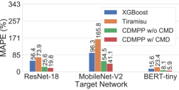
(a) Cross-model learning on T4

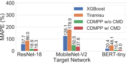
(b) Cross-model learning on EPYC

Figure 15. Comparison of cross-model prediction errors. The number on top of each bar is the exact MAPE value.

(a) BERT-tiny, w/o CMD

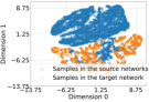
(b) BERT-tiny, w/ CMD

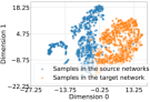
(c) MobileNet-V2, w/o CMD

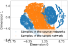
(d) MobileNet-V2, w/ CMD

Figure 16. Hidden representation comparison with t-SNE.

Fig. 15 shows more results for cross-model fine-tuning. In most cases, CDMPP can achieve a small prediciton error. However, in some cases, e.g., when taking MobileNet-V2 as the target network, the prediction error is large for all methods, because the distribution shift between the source and target domain is too large for domain adaption technique to mitigate, as shown in Fig. 16(c). In this case, we recommend augmenting the training set to cover more samples.

D.2. End2end performance for CMPP

Fig. 17 evaluates the cross-model prediction error of end-to-end performance against the real performance on various devices. The results show that CDMPP can accurately estimate the latency with an error at most $12.4\%$ and outperform all the baselines.

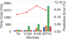
(a) Predicted onto ResNet50, BS=1

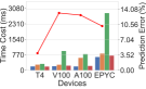
(b) Predicted onto ResNet50, BS=4

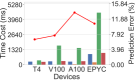
(c) Predicted onto ResNet50, BS=8

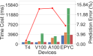
(d) Predicted onto InceptionV3, BS=1

(e) Predicted onto BERT Base, BS=1

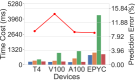
(f) Predicted onto BERT Base, BS=4

Figure 17. End-to-end performance prediction for cross-model learning.

D.3. Effect of distribution difference on model generalizability

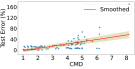
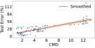
Figure 18. Effect of distribution difference on model generalizability. x-axis: CMD between $X_{train}$ and $X_{test}$ subsets, y-axis: corresponding test error of the subset of $X_{test}$: a) Cross-model learning, where both $X_{train}$ and $X_{test}$ are collected from T4; b) Cross-device learning, where$X_{train}$ and $X_{test}$ are collected from different devices

To illustrate the effects of distribution difference (measured as CMD) on prediction performance, we plot the CMD (x-axis) between two subsets that are randomly sampled from the training set and test set respectively, and the corresponding prediction error (y-axis), for both cross-model and cross-device training in Fig. 18. The performance of the predictor is positively related to prediction error, which indicates a predictor trained on one distribution can be well generalized to another distribution that has a small CMD difference from the training distribution.

Appendix E Artifact Appendix

E.1. Abstract

CDMPP is a generic optimized framework for precise performance prediction of tensor programs across diverse DNN models and devices. We provide the source code of CDMPP for artifact evaluation, which implements data preprocessing, cost model training, and model inference.

E.2. Description & Requirements

E.2.1. How to access

You can access the source code of CDMPP at this Github Repo: https://github.com/joapolarbear/cdmpp.The dataset and source code is also available at DOI:10.6084/m9.figshare.24156084

E.2.2. Hardware dependencies

The current implementation of CDMPP requires GPUs to run the cost model.

E.2.3. Software dependencies

• customized TVM: https://github.com/joapolarbear/tvm

• dPRO: https://github.com/joapolarbear/dpro

• CUDA driver version ¿=450.80.02 (Linux) / 452.39 (Windows)

E.2.4. Benchmarks

Dataset: You can access the dataset through the following links:

• $dataset\_cpu\_v3.3.zip$: https://drive.google.com/file/d/1JQwGEe8jCpuhZPnUxO0Sb1CJJ06uevy6/view

• $dataset\_gpu\_v3.3.zip$: https://drive.google.com/file/d/1jqHbmvXUrLPDCIqJIaPee_atsPc0ZFFK/view

You can choose to use either the CPU part or the GPU part. Please follow the instructions in [Tenset Dataset](https://github.com/tlc-pack/tenset/blob/main/docs/get_started_with_cost_model_experiments.md) to download the dataset accordingly. Our profiled dataset for A100, V100 and P100 will be available at [figshare](10.6084/m9.figshare.24156084)

E.3. Set-up

E.3.1. Software Environment

Pull the docker image

⬇

docker pull haaanpeng/cdmpp:eurosys_ae

Launch the container

⬇

docker run -it --runtime=nvidia --shm-size 32768m --name hphu-test haaanpeng/cdmpp:eurosys_ae /bin/bash

Download the source code and install dependencies.

⬇

cd && git clone --recursive https://github.com/joapolarbear/cdmpp && cd cdmpp && bash setup.sh

E.4. Prepare Dataset

E.4.1. Download and unzip

You can choose to use either the CPU part or the GPU part. See [Tenset Dataset](https://github.com/tlc-pack/tenset/blob/main/docs/get_started_with_cost_model_experiments.md) to download the dataset accordingly. Our profiled dataset for A100, V100 and P100 will be available at [DOI:10.6084/m9.figshare.24156084](https://figshare.com/articles/dataset/cdmpp-data/24156084)

An example of T4 GPU. Here we show an example of downloading the dataset of NVIDIA T4.

1. Change directory to <cdmpp_root_directory>/3rdparty/tenset/scripts/

2. Download. You can download it from Google Drive with the link [$dataset\_gpu\_v3.3.zip$](https://drive.google.com/file/d/1jqHbmvXUrLPDCIqJIaPee_atsPc0ZFFK/view?usp=sharing). Or you can use the command line

   ⬇

   pip3 install gdown

   gdown https://drive.google.com/uc?

   id=1jqHbmvXUrLPDCIqJIaPee_atsPc0ZFFK

3. Unzip. Put dataset_gpu_v3.3.zip under <cdmpp_root_directory>/3rdparty/tenset/scripts/ and run unzip dataset_gpu_v3.3.zip. A new folder <dataset_gpu> will appear in <cdmpp_root_directory>/3rdparty/tenset/scripts/. Make dataset as a soft link to it by the following command

   ⬇

   ln -s <cdmpp_root_directory>/3rdparty/tenset/

   scripts/dataset_gpu dataset

An example of AMD EPYC 7452 CPU. Here we show an example to download the dataset of AMD EPYC 7452 CPU.

1. Change directory to <cdmpp_root_directory>/3rdparty/tenset/scripts/

2. Download. You can download it from Google Drive with the link [dataset_cpu_v3.3.zip](https://drive.google.com/file/d/1JQwGEe8jCpuhZPnUxO0Sb1CJJ06uevy6/view?usp=sharing). Or you can use the command line

   ⬇

   pip3 install gdown

   gdown https://drive.google.com/uc?

   id=1JQwGEe8jCpuhZPnUxO0Sb1CJJ06uevy6

3. Unzip. Put dataset_cpu_v3.3.zip under <cdmpp_root_directory>/3rdparty/tenset/scripts/ and run unzip dataset_cpu_v3.3.zip. A new folder <dataset_cpu> will appear in <cdmpp_root_directory>/3rdparty/tenset/scripts/. Make dataset as a soft link to it by the following command

   ⬇

   ln -s <cdmpp_root_directory>/3rdparty/tenset/

   scripts/dataset_cpu dataset

In the above process, if dataset already exists, just run

⬇

mv dataset_cpu/measure_records/* dataset/measure_records/

After the above processes, you will see several directories under <cdmpp_root_directory>/3rdparty/tenset/scripts/dataset/measure_records as follows

⬇

measure_records

|-t4

|-k80

Note that each directory name represents a specific device and we will use those device names as flags to specify which device we will use to extract features or run training.

E.4.2. Feature Extraction.

After downloading the dataset and putting it on the right path, we will extract features for the dataset of each device. Make sure that you have put the profiled dataset under 3rdparty/tenset/scripts/dataset/measure_records/<DEVICE_MODEL>, where <DEVICE_MODEL> is the device whose dataset you want to extract from. Then, you can run the following commands to extract features.

⬇

cd && cd cdmpp

bash scripts/dataset/gen_raw_feature_all.sh

By default, the extracted features will be stored at workspace/ast_ansor/<DEVICE_MODEL>. The process of extracting features and data preprocessing may take around $10\sim 20$ minutes for the dataset of each device.

E.4.3. Data Preprocessing [Optional].

Run the following commands to preprocess the dataset

⬇

bash scripts/dataset/make_dataset.sh

The preprocessed data will be stored under the tmp/ directory. You can also skip this process since this can be done automatically before training starts, i.e., when the preprocessed dataset is required to be used for the first time. This step takes around 5 minutes for the dataset of each device.

E.5. Evaluation workflow

We mainly shows an example of the process to evaluate cross-model performance prediction, with the dataset collected from T4.

E.5.1. Major Claims

• (C1): CDMPP can achieve a prediction error around $19\%$ [refer to Fig. 7-(a) in the paper].

E.5.2. Experiments

Experiment (E1): [CMPP] [5 human-minutes + $3\sim 5$ GPU compute-hour]: cross model cost model training on the dataset from T4

[How to]
Please follow the steps to perform this experiments  
[Preparation] We will use the configuration file tmp/search_trial_20221119_1575.yaml, which contains hyper-parameters found by our auto-tuner, to run the following experiments. You can also change the hyper-parameters in the configuration file according to your requirements.  
[Execution] Run the following commands

⬇

bash scripts/exp/cross_model.sh none

[Results] You will see training logs like this

⬇

[2023-09-30 13:53:55] [base_learner.py:303] INFO - Time 1240.564 s - Epoch 126 step 27000 bs 600 - loss_train=17.410308837891, {’mape’: 0.2110657768101716, ’rmse’: 0.00045307391267025536, ’20%accuracy’: 0.6356699751861042, ’10%accuracy’: 0.3441997518610422, ’5%accuracy’: 0.17478287841191067}

After training converges, the MAPE should be around 0.19, indicating $19\%$ test error.

References

- [1] Martín Abadi, Paul Barham, Jianmin Chen, Zhifeng Chen, Andy Davis, Jeffrey Dean, Matthieu Devin, Sanjay Ghemawat, Geoffrey Irving, Michael Isard, et al. Tensorflow: A System for Large-scale Machine Learning. In Proceedings of the 12th USENIX Symposium on Operating Systems Design and Implementation, 2016.
- [2] Andrew Adams, Karima Ma, Luke Anderson, Riyadh Baghdadi, Tzu-Mao Li, Michaël Gharbi, Benoit Steiner, Steven Johnson, Kayvon Fatahalian, Frédo Durand, et al. Learning to optimize halide with tree search and random programs. ACM Transactions on Graphics (TOG), 2019.
- [3] Takuya Akiba, Shotaro Sano, Toshihiko Yanase, Takeru Ohta, and Masanori Koyama. Optuna: A Next-generation Hyperparameter Optimization Framework. In Proceedings of the 25th ACM SIGKDD International Conference on Knowledge Discovery and Data Mining, 2019.
- [4] AMD. AMD EPYC, 2019. https://www.amd.com/en/products/cpu/amd-epyc-7452.
- [5] Riyadh Baghdadi, Massinissa Merouani, Mohamed-Hicham Leghettas, Kamel Abdous, Taha Arbaoui, Karima Benatchba, et al. A deep learning based cost model for automatic code optimization. In Proceedings of Machine Learning and Systems, 2021.
- [6] Anna C Belkina, Christopher O Ciccolella, Rina Anno, Richard Halpert, Josef Spidlen, and Jennifer E Snyder-Cappione. Automated optimized parameters for T-distributed stochastic neighbor embedding improve visualization and analysis of large datasets. Nature communications, 2019.
- [7] George EP Box and David R Cox. An analysis of transformations. Journal of the Royal Statistical Society: Series B (Methodological), 1964.
- [8] Lars Buitinck, Gilles Louppe, Mathieu Blondel, Fabian Pedregosa, Andreas Mueller, Olivier Grisel, Vlad Niculae, Peter Prettenhofer, Alexandre Gramfort, Jaques Grobler, Robert Layton, Jake VanderPlas, Arnaud Joly, Brian Holt, and Gaël Varoquaux. API design for machine learning software: experiences from the scikit-learn project. In ECML PKDD Workshop: Languages for Data Mining and Machine Learning, 2013.
- [9] Han Cai, Ligeng Zhu, and Song Han. Proxylessnas: Direct neural architecture search on target task and hardware. arXiv preprint arXiv:1812.00332, 2018.
- [10] Tianqi Chen, Tong He, Michael Benesty, Vadim Khotilovich, Yuan Tang, Hyunsu Cho, Kailong Chen, et al. Xgboost: extreme gradient boosting. R package version 0.4-2, 2015.
- [11] Tianqi Chen, Thierry Moreau, Ziheng Jiang, Lianmin Zheng, Eddie Yan, Haichen Shen, Meghan Cowan, Leyuan Wang, Yuwei Hu, Luis Ceze, et al. TVM: An Automated End-to-End Optimizing Compiler for Deep Learning. In Proceedings of the 13th USENIX Symposium on Operating Systems Design and Implementation, 2018.
- [12] Tianqi Chen, Lianmin Zheng, Eddie Yan, Ziheng Jiang, Thierry Moreau, Luis Ceze, Carlos Guestrin, and Arvind Krishnamurthy. Learning to optimize tensor programs. In Proceedings of Advances in Neural Information Processing Systems, 2018.
- [13] NVIDIA Corporation. NVIDIA K80, 2014. https://www.nvidia.com/en-gb/data-center/tesla-k80/.
- [14] NVIDIA Corporation. NVIDIA P100, 2016. https://www.nvidia.com/en-sg/data-center/tesla-p100/.
- [15] NVIDIA Corporation. NVIDIA V100, 2017. https://www.nvidia.com/en-gb/data-center/tesla-v100/.
- [16] NVIDIA Corporation. NVIDIA 2080Ti, 2018. https://www.nvidia.cn/geforce/graphics-cards/rtx-2080-ti/.
- [17] NVIDIA Corporation. NVIDIA T4, 2018. https://www.nvidia.com/en-in/data-center/tesla-t4/.
- [18] NVIDIA Corporation. NVIDIA A100, 2020. https://www.nvidia.com/en-sg/data-center/a100/.
- [19] NVIDIA Corporation. NVIDIA Data Center Deep Learning Product Performance, 2020. https://developer.nvidia.com/deep-learning-performance-training-inference.
- [20] Zihang Dai, Zhilin Yang, Yiming Yang, Jaime Carbonell, Quoc V Le, and Ruslan Salakhutdinov. Transformer-xl: Attentive language models beyond a fixed-length context. arXiv preprint arXiv:1901.02860, 2019.
- [21] Anirban DasGupta. Probability for statistics and machine learning: fundamentals and advanced topics. Springer, 2011.
- [22] Jacob Devlin, Ming-Wei Chang, Kenton Lee, and Kristina Toutanova. Bert: Pre-training of deep bidirectional transformers for language understanding. arXiv preprint arXiv:1810.04805, 2018.
- [23] Lukasz Dudziak, Thomas Chau, Mohamed Abdelfattah, Royson Lee, Hyeji Kim, and Nicholas Lane. BRP-NAS: Prediction-based NAS using GCNS. In Proceedings of Advances in Neural Information Processing Systems, 2020.
- [24] Amazon EC2. AWS Graviton Processor, 2019. https://aws.amazon.com/cn/ec2/graviton/.
- [25] X Yu Geoffrey, Yubo Gao, Pavel Golikov, and Gennady Pekhimenko. Habitat: A Runtime-Based Computational Performance Predictor for Deep Neural Network Training. In Proceedings of the 2021 USENIX Annual Technical Conference, 2021.
- [26] Google. Tensor Processing Unit, 2016. https://cloud.google.com/tpu/docs/tpus.
- [27] Kaiming He, Xiangyu Zhang, Shaoqing Ren, and Jian Sun. Deep Residual Learning for Image Recognition. In Proceedings of the IEEE conference on Computer Vision and Pattern Recognition, 2016.
- [28] Kevin Hsieh, Amar Phanishayee, Onur Mutlu, and Phillip Gibbons. The non-iid data quagmire of decentralized machine learning. In Proceedings of International Conference on Machine Learning, 2020.
- [29] Hanpeng Hu, Chenyu Jiang, Yuchen Zhong, Yanghua Peng, Chuan Wu, Yibo Zhu, Haibin Lin, and Chuanxiong Guo. dPRO: A Generic Profiling and Optimization System for Expediting Distributed DNN Training. In Proceedings of Machine Learning and Systems, 2022.
- [30] HUAWEI. HUAWEI Ascend, 2018. https://e.huawei.com/cn/products/servers/ascend.
- [31] Intel. Intel® Xeon® Processor E5-2673 v4, 2016. https://ark.intel.com/content/www/us/en/ark/products/series/91287/intel-xeon-processor-e5-v4-family.html.
- [32] Intel. Intel Platinum, 2019. https://www.intel.sg/content/www/xa/en/products/details/processors/xeon/scalable/platinum.html.
- [33] Zhihao Jia, Oded Padon, James Thomas, Todd Warszawski, Matei Zaharia, and Alex Aiken. TASO: Optimizing Deep Learning Computation with Automatic Generation of Graph Substitutions. In Proceedings of the 27th ACM Symposium on Operating Systems Principles, 2019.
- [34] Zhihao Jia, James Thomas, Todd Warszawski, Mingyu Gao, Matei Zaharia, and Alex Aiken. Optimizing DNN computation with relaxed graph substitutions. In Proceedings of Machine Learning and Systems, 2019.
- [35] Zhihao Jia, Matei Zaharia, and Alex Aiken. Beyond Data and Model Parallelism for Deep Neural Networks. In Proceedings of Machine Learning and Systems, 2019.
- [36] Abhinav Ramesh Kashyap, Devamanyu Hazarika, Min-Yen Kan, and Roger Zimmermann. Domain Divergences: a Survey and Empirical Analysis, 2020.
- [37] Sam Kaufman, Phitchaya Phothilimthana, Yanqi Zhou, Charith Mendis, Sudip Roy, Amit Sabne, and Mike Burrows. A learned performance model for tensor processing units. In Proceedings of Machine Learning and Systems, 2021.
- [38] Samuel Kaufman, Phitchaya Mangpo Phothilimthana, and Mike Burrows. Learned TPU cost model for XLA tensor programs. In Proc. Workshop ML Syst. NeurIPS, 2019.
- [39] Jack Kosaian, Amar Phanishayee, Matthai Philipose, Debadeepta Dey, and Rashmi Vinayak. Boosting the throughput and accelerator utilization of specialized cnn inference beyond increasing batch size. In Proceedings of International Conference on Machine Learning, 2021.
- [40] Habana Labs. Habana Goya, 2019. https://habana.ai/.
- [41] Chris Lattner, Mehdi Amini, Uday Bondhugula, Albert Cohen, Andy Davis, Jacques Pienaar, River Riddle, Tatiana Shpeisman, Nicolas Vasilache, and Oleksandr Zinenko. MLIR: A compiler infrastructure for the end of Moore’s law. arXiv preprint arXiv:2002.11054, 2020.
- [42] Ji Lin, Wei-Ming Chen, Yujun Lin, Chuang Gan, Song Han, et al. Mcunet: Tiny deep learning on iot devices. In Proceedings of Advances in Neural Information Processing Systems, 2020.
- [43] Liang Liu, Mingzhu Shen, Ruihao Gong, Fengwei Yu, and Hailong Yang. NNLQP: A Multi-Platform Neural Network Latency Query and Prediction System with An Evolving Database. In Proceedings of the 51st International Conference on Parallel Processing, 2022.
- [44] Mingsheng Long, Han Zhu, Jianmin Wang, and Michael I. Jordan. Deep Transfer Learning with Joint Adaptation Networks, 2016.
- [45] Peter Mattson, Christine Cheng, Gregory Diamos, Cody Coleman, Paulius Micikevicius, David Patterson, Hanlin Tang, Gu-Yeon Wei, Peter Bailis, Victor Bittorf, et al. Mlperf training benchmark. In Proceedings of Machine Learning and Systems, 2020.
- [46] Peter Meltzer, Marcelo Daniel Gutierrez Mallea, and Peter J Bentley. Pinet: A permutation invariant graph neural network for graph classification. arXiv preprint arXiv:1905.03046, 2019.
- [47] MLPerf. MLPerf, 2020. https://mlcommons.org/.
- [48] Mehdi Mohammadi, Ala Al-Fuqaha, Sameh Sorour, and Mohsen Guizani. Deep learning for IoT big data and streaming analytics: A survey. IEEE Communications Surveys & Tutorials, 2018.
- [49] NVIDIA. CUDA Toolkit Release Notes, 2020. https://docs.nvidia.com/cuda/archive/10.2/cuda-toolkit-release-notes/index.html.
- [50] NVIDIA. cuDNN Documentation, 2021. https://docs.nvidia.com/deeplearning/cudnn/developer-guide/index.html.
- [51] Adam Paszke, Sam Gross, Soumith Chintala, Gregory Chanan, Edward Yang, Zachary DeVito, Zeming Lin, Alban Desmaison, Luca Antiga, and Adam Lerer. Automatic differentiation in PyTorch. In NIPS-W, 2017.
- [52] Adam Paszke, Sam Gross, Francisco Massa, Adam Lerer, James Bradbury, Gregory Chanan, Trevor Killeen, Zeming Lin, Natalia Gimelshein, Luca Antiga, et al. PyTorch: An Imperative Style, High-performance Deep Learning Library. In Proceedings of Advances in Neural Information Processing Systems, 2019.
- [53] Leonardo Petrini, Francesco Cagnetta, Eric Vanden-Eijnden, and Matthieu Wyart. Learning sparse features can lead to overfitting in neural networks. arXiv preprint arXiv:2206.12314, 2022.
- [54] Hieu Pham, Melody Guan, Barret Zoph, Quoc Le, and Jeff Dean. Efficient neural architecture search via parameters sharing. In Proceedings of International Conference on Machine Learning, 2018.
- [55] Vijay Janapa Reddi, Christine Cheng, David Kanter, Peter Mattson, Guenther Schmuelling, Carole-Jean Wu, Brian Anderson, Maximilien Breughe, Mark Charlebois, William Chou, et al. Mlperf inference benchmark. In 2020 ACM/IEEE 47th Annual International Symposium on Computer Architecture (ISCA), 2020.
- [56] Ievgen Redko, Emilie Morvant, Amaury Habrard, Marc Sebban, and Younès Bennani. A survey on domain adaptation theory: learning bounds and theoretical guarantees. arXiv preprint arXiv:2004.11829, 2020.
- [57] Jaehun Ryu and Hyojin Sung. Metatune: Meta-learning based cost model for fast and efficient auto-tuning frameworks. arXiv preprint arXiv:2102.04199, 2021.
- [58] Karen Simonyan and Andrew Zisserman. Very Deep Convolutional Networks for Large-Scale Image Recognition. In Proceedings of International Conference on Learning Representations, 2015.
- [59] Benoit Steiner, Chris Cummins, Horace He, and Hugh Leather. Value learning for throughput optimization of deep learning workloads. In Proceedings of Machine Learning and Systems, 2021.
- [60] Petar Stojanov, Zijian Li, Mingming Gong, Ruichu Cai, Jaime G. Carbonell, and Kun Zhang. Domain Adaptation with Invariant Representation Learning: What Transformations to Learn? In Proceedings of Advances in Neural Information Processing Systems, 2021.
- [61] Jie Tang, Dawei Sun, Shaoshan Liu, and Jean-Luc Gaudiot. Enabling deep learning on IoT devices. IEEE Computer, 2017.
- [62] Ashish Vaswani, Noam Shazeer, Niki Parmar, Jakob Uszkoreit, Llion Jones, Aidan N Gomez, Ł ukasz Kaiser, and Illia Polosukhin. Attention is all you need. In Proceedings of Advances in Neural Information Processing Systems, 2017.
- [63] Yidong Wang, Bowen Zhang, Wenxin Hou, Zhen Wu, Jindong Wang, and Takahiro Shinozaki. Margin calibration for long-tailed visual recognition. In Proceedings of Asian Conference on Machine Learning, 2023.
- [64] Sanford Weisberg. Yeo-Johnson power transformations. Department of Applied Statistics, University of Minnesota. Retrieved June, 2001.
- [65] Samuel Williams, Andrew Waterman, and David Patterson. Roofline: an insightful visual performance model for multicore architectures. Communications of the ACM, 2009.
- [66] Yang You, Zhao Zhang, Cho-Jui Hsieh, James Demmel, and Kurt Keutzer. Fast deep neural network training on distributed systems and cloud TPUs. IEEE Transactions on Parallel and Distributed Systems, 2019.
- [67] Werner Zellinger, Bernhard A Moser, Thomas Grubinger, Edwin Lughofer, Thomas Natschläger, and Susanne Saminger-Platz. Robust unsupervised domain adaptation for neural networks via moment alignment. Information Sciences, 2019.
- [68] Yi Zhai, Yu Zhang, Shuo Liu, Xiaomeng Chu, Jie Peng, Jianmin Ji, and Yanyong Zhang. TLP: A Deep Learning-Based Cost Model for Tensor Program Tuning. In Proceedings of the 28th ACM International Conference on Architectural Support for Programming Languages and Operating Systems, 2023.
- [69] Li Lyna Zhang, Shihao Han, Jianyu Wei, Ningxin Zheng, Ting Cao, Yuqing Yang, and Yunxin Liu. nn-Meter: towards accurate latency prediction of deep-learning model inference on diverse edge devices. In Proceedings of the 19th Annual International Conference on Mobile Systems, Applications, and Services, 2021.
- [70] Zhihe Zhao, Xian Shuai, Yang Bai, Neiwen Ling, Nan Guan, Zhenyu Yan, and Guoliang Xing. Moses: Efficient Exploitation of Cross-device Transferable Features for Tensor Program Optimization. arXiv preprint arXiv:2201.05752, 2022.
- [71] Lianmin Zheng, Chengfan Jia, Minmin Sun, Zhao Wu, Cody Hao Yu, Ameer Haj-Ali, Yida Wang, Jun Yang, Danyang Zhuo, Koushik Sen, et al. Ansor: Generating High-Performance Tensor Programs for Deep Learning. In Proceedings of the 14th USENIX Symposium on Operating Systems Design and Implementation, 2020.
- [72] Lianmin Zheng, Ruochen Liu, Junru Shao, Tianqi Chen, Joseph E Gonzalez, Ion Stoica, and Ameer Haj Ali. Tenset: A large-scale program performance dataset for learned tensor compilers. In Proceedings of the Thirty-fifth Conference on Neural Information Processing Systems Datasets and Benchmarks Track, 2021.
- [73] Hongyu Zhu, Mohamed Akrout, Bojian Zheng, Andrew Pelegris, Anand Jayarajan, Amar Phanishayee, Bianca Schroeder, and Gennady Pekhimenko. Benchmarking and analyzing deep neural network training. In 2018 IEEE International Symposium on Workload Characterization (IISWC), 2018.
- [74] Qi Zhu, Natalia Ponomareva, Jiawei Han, and Bryan Perozzi. Shift-Robust GNNs: Overcoming the Limitations of Localized Graph Training Data, 2021.