An inexact Matrix-Newton method for solving NEPv

Abstract

Our main contribution in this paper is to present an inexact Matrix-Newton algorithm that uses the tools for Newton’s method in Banach spaces to solve a particular type of matrix valued problem: the nonlinear eigenvalue problem with eigenvector dependency (NEPv). We provide the conditions for our algorithm to be applicable to NEPv and show how to exploit the problem structure for an efficient implementation. Various numerical experiments are provided that indicate the advantage of quadratic order of convergence over the linear order of the well-established SCF algorithm.

1. Introduction

In this paper, we consider eigenvector-dependent nonlinear eigenvalue problems (NEPv) to be formulated in the following form: given some matrix function $H:\mathbb{C}^{n,k}\rightarrow\mathbb{C}^{n,n}$ with $H(V)=H(V)^{H}$,

$$\text{find }V\in\mathrm{U}_{n,k}(\mathbb{C})\text{ and }\Lambda=\Lambda^{H}\in\mathbb{C}^{k,k}\text{ such that }H(V)V=V\Lambda,$$ (1)

where $\mathrm{U}_{n,k}(\mathbb{C})$ denotes the set of $n\times k$ complex matrices with orthonormal columns and $X^{H}$ denotes the conjugate transpose of $X\in\mathbb{C}^{n,k}$. The (1) arises in a variety of applications, most notably in the discretized Kohn-Sham-equation [23, 26], the Gross-Pitaevski equation [5, 18] as well as in data analysis applications for the trace ratio or robust Rayleigh quotient optimization problems used in linear discriminant analysis [4, 7, 24, 30]. In most of those cases, the eigenvalue problem is closely related to a minimization problem with orthogonality constraints and appears as an equivalent formulation to the original problem when analyzing its first order optimality conditions (KKT-conditions) [4, 8, 29].
One can show that (1) has a unique solution, if there is a uniform gap between the $k$-th and $(k+1)$-st eigenvalue of $H(V)$, for any $V\in\mathrm{U}_{n,k}(\mathbb{C})$, and $H$ satisfies some form of Lipschitz-condition [8, Thm. 1]. However, it is worth noting that most functions of interest satisfy

$$H(V)\equiv H(VQ),\quad\text{for any }Q\in\mathrm{U}_{k}(\mathbb{C}),$$

meaning that uniqueness of solutions can only be achieved up to unitary transformations.
Sometimes, (1) is modified by an additional matrix function $G:\mathbb{C}^{n,k}\rightarrow\mathbb{C}^{n,n}$, $G(V)=G(V)^{H}$, leading to what we will call the generalized NEPv (GNEPv):

$$\text{Find }V\in\mathrm{U}_{n,k}(\mathbb{C})\text{ and }\Lambda=\Lambda^{H}\in\mathbb{C}^{k,k}\text{ such that }H(V)V=G(V)V\Lambda.$$ (2)

Certainly, whenever $(V,\Lambda)$ satisfies (1), the eigenvalues of $\Lambda$ are eigenvalues of $H(V)$. In most practical applications, one is therefore interested in finding $V\in\mathrm{U}_{n,k}(\mathbb{C})$ with $H(V)V=V\Lambda$ such that the eigenvalues of $\Lambda$ become as large/small as possible.
One popular method to solve this problem is the self-consistent-field iteration (SCF algorithm, see LABEL:alg:plainscf) originating from electronic structure calculations, where it is commonly used to solve Hartree-Fock or Kohn-Sham equations [23, 26, 28]. In this simple iterative scheme, a new iterate $V_{j+1}$ is generated by computing the desired eigenpairs of $H_{j}=H(V_{j})$ until the iteration becomes stationary.

Input: $V_{0}\in\mathrm{U}_{n\times k}(\mathbb{C})$, $H:\mathbb{C}^{n,k}\rightarrow\mathbb{C}^{n,n}$

Output: $(V^{*},\Lambda^{*})\in\mathbb{C}^{n,k}\times\mathbb{C}^{k,k}$ approximate solution to $H(V)V=V\Lambda$

1 Set $j=0$

2 while not converged do

3       Evaluate $H_{j}=H(V_{j})$

4       Compute $(V_{j+1},\Lambda_{j+1})$ as the $k$ largest/smallest eigenpairs of $H_{j}$

5       Set $j=j+1$

6      

Return $(V^{*},\Lambda^{*})=(V_{j},\Lambda_{j})$ algorithm]alg:plainscf

Algorithm 1 Plain SCF

Another approach to solve (1), first considered by Gao, Yang and Meza [14], is the use of Newton’s method. They rewrote the eigenvalue problem (1) as a root finding problem $F(X)=0$ with

$$F:\mathbb{C}^{n,k}\times\mathbb{C}^{k,k}\rightarrow\mathbb{C}^{n+k,k},\text{ }F(V,\Lambda)=\begin{bmatrix}H(V)V-V\Lambda\\ V^{H}V-I_{k}\end{bmatrix}$$ (3)

which was considered in its vectorized form $f(x)=0$ as

$$f:\mathbb{C}^{n\cdot k}\times\mathbb{C}^{k\cdot k}\rightarrow\mathbb{C}^{(n+k)\cdot k},\text{ }f(\mathop{\mathrm{vec}}(V),\mathop{\mathrm{vec}}(\Lambda))=\begin{bmatrix}\mathop{\mathrm{vec}}(H(V)V-V\Lambda)\\ \mathop{\mathrm{vec}}(V^{H}V-I_{k})\end{bmatrix}$$

and solved using a vector Newton approach. Here, we denote by $\mathop{\mathrm{vec}}(\cdot)$ the operator that stacks the columns of a matrix vertically.
The algorithm was discussed for a discretized Kohn-Sham-modell for which the Jacobian $J_{f}(x_{k})$ could be explicitly determined and could be shown to outperform the SCF-approach for relatively small dimensions when exploiting the structure of the problem. In this paper, we want to follow a similar route by using a Newton approach for the matrix valued problem (3). This way, we can avoid vectorizing the problem and work with the original matrix problem structure. This allows for an efficient iterative solve of the update equation using block Krylov methods.
The following chapters are organized as follows: in Chapter 2, we derive the general framework for solving matrix valued root finding problems by Newton’s method. For this sake, we introduce an inexact Newton method using a global GMRES approach for approximately solving the Newton update equation. In Chapter 3, we demonstrate how to apply the inexact Newton algorithm to (1) or (2) efficiently. In Chapter 4, we apply the newly derived algorithm to several test problems from different applciations and compare its convergence speed to the SCF algorithm. We finish off with a discussion of our results and a summary of our contribution in Chapter 5.

2. Newton’s Method for nonlinear matrix equations

In this section, we consider the problem of finding a root $X^{*}\in\mathbb{C}^{n,k}$ of a matrix function $F:\mathbb{C}^{n,k}\rightarrow\mathbb{C}^{n,k}$. In the simple case where $k=1$ and $F$ is differentiable, this problem can be solved by the well-known multivariate Newton method [2], which requires the update

$$x_{j+1}=x_{j}-J_{F}(x_{j})^{-1}F(x_{j}),$$

where $J_{F}(x_{j})\in\mathbb{C}^{n,n}$ is the Jacobian of $F$ at $x_{j}\in\mathbb{C}^{n}$. Usually, the explicit inversion of the Jacobian is avoided by rewriting the update formula in the form

$$J_{F}(x_{j})e_{j}=-F(x_{j}),\quad x_{j+1}=x_{j}+e_{j},$$ (4)

where a linear system with the Jacobian is solved to obtain the update direction $e_{j}$. A similar approach to (4) is possible for matrix functions ($k>1$) using the Fréchet derivative of $F$ instead of the Jacobian to perform the update

$$L_{F}(X_{j},E_{j})=-F(X_{j}),\quad X_{j+1}=X_{j}+E_{j},$$ (5)

where $L_{F}(X_{j},E_{j})$ is the Fréchet derivative of $F$ at $X_{j}$ in direction of $E_{j}$.

Definition 1 (Fréchet derivative and Kronecker form).

The Fréchet derivative of a matrix function $F:\mathbb{C}^{n,k}\rightarrow\mathbb{C}^{n,k}$ at a point $X$, if it exists, is the unique linear mapping

$$L_{F}(X):\mathbb{C}^{n,k}\rightarrow\mathbb{C}^{n,k},\quad E\mapsto L_{F}(X)(E)\mathop{\coloneqq}L_{F}(X,E),$$

such that for every $E\in\mathbb{C}^{n,k}$ it holds

$$F(X+E)-F(X)-L_{F}(X,E)=\mathop{o}(\lVert E\rVert).$$

Since $L_{F}(X)$ is a linear operator, there exists $K_{F}(X)\in\mathbb{C}^{n\cdot k,n\cdot k}$ not depending on $E$ such that

$$\mathop{\mathrm{vec}}(L_{F}(X,E))=K_{F}(X)\mathop{\mathrm{vec}}(E).$$

We refer to $K_{F}(X)$ as the Kronecker form of the Fréchet derivative.

It is straightforward to show that the classic rules for differentiating composed functions apply to the Fréchet derivative in the same way, most notably the product and chain rule [17, Sec. 3.2].
As the Fréchet derivative is linear in $E$, solving a linear matrix equation is required to find the update direction $E_{j}$ in (5). Certainly, similar to the scalar and vector-valued case, Newton’s method in the form (5) can be shown to converge quadratically in a neighbourhood around a root $X^{*}\in\mathbb{C}^{n,k}$ of $F$ as long as $F$ is Fréchet differentiable and the update equation $L_{F}(X_{j},E_{j})=-F(X_{j})$ has a unique solution for every $X_{j}$ [6].
Since solving the equation directly for $E$ is usually challenging due to the Fréchet derivative being complicated, we have to settle for approximate solutions to the update equation which we can compute by iterative methods, leading to a class of algorithms called inexact Newton methods (INM) which we will briefly introduce in the following section.

2.1. Inexact Newton methods

In the inexact Newton framework, we seek to find an update direction $E_{j}$ by finding a matrix satisfying the residual inequality

$$\lVert R_{j}(E_{j})\rVert_{F}\leq\eta_{j}\lVert F(X_{j})\rVert_{F},\quad\eta_{j}>0,$$ (6)

where $R_{j}(E_{j})\mathop{\coloneqq}L_{F}(X_{j},E_{j})+F(X_{j})$ is the residual of the update equation (5) and $\eta_{j}$ is the so-called forcing term affecting the relative accuracy at which the equation is solved [12, 13]. Since $L_{F}(X)$ is linear, a solution $E_{j}$ of (6) can be computed by employing iterative solvers for linear equations, in particular Krylov subspace methods. Note that in the Krylov subspace setting, we usually do not need to know the exact derivative of $F$ to be able to extend the subspace, we only need to be able to apply the derivative in a given direction, which can be done by finite difference approximations. In the case of vector-valued functions, approaches combining inexact Newton methods with Krylov subspace methods as inner solver are referred to as (Jacobian-free) Newton-Krylov methods (JFNK) [21].
To get more insight on how to apply JFNK to matrix-valued problems, consider again the Newton update equation (5) and its vectorized companion

$$K_{F}(X_{j})\mathop{\mathrm{vec}}(E_{j})=-\mathop{\mathrm{vec}}(F(X_{j}))$$ (7)

using the Kronecker form of the Fréchet derivative. In theory, $E_{j}$ can be computed by employing GMRES for the vectorized equation (7), where we have to compute the matrix-vector products $K_{F}(X_{j})\cdot v_{l}$ to expand the Arnoldi sequence. However, computing $K_{F}(X_{j})$ explicitly is not appropriate in this application, since the computation itself is expensive and the resulting problem is way bigger than the original matrix-valued problem.
Instead, we want to view (5) as a system of linear equations with multiple right-hand sides

$$AY=B,\quad A\in\mathbb{C}^{n,n},\;Y,B\in\mathbb{C}^{n,k},$$

and follow a global GMRES approach [19]. In the global GMRES-algorithm, we seek to find an approximate solution to $AY=B$ by spanning the matrix Krylov subspace

$$\mathcal{K}_{\ell}(A,B)=\textnormal{{span}}\{B,AB,A^{2}B,\dots,A^{\ell-1}B\}$$

with a series of matrices $\{V_{1},V_{2},\dots,V_{l}\}$ generated from a global Arnoldi-process that are orthogonal to each other with respect to the Frobenius scalar product $\langle X,Y\rangle_{F}=\mathop{\mathrm{tr}}(X^{H}Y)$ and normalized, i.e. $\langle V_{i},V_{j}\rangle_{F}=\delta_{i,j}$ and satisfy the relation

$$A\mathcal{V}_{\ell}=\mathcal{V}_{\ell+1}(\underline{H}_{\ell}\otimes I_{k}),$$

where $\mathcal{V}_{\ell}=\left[V_{1},V_{2},\dots,V_{\ell}\right]\in\mathbb{C}^{n,k\cdot\ell}$ and $\underline{H}_{\ell}\in\mathbb{C}^{\ell+1,\ell}$ is upper Hessenberg with an additional row and entries $h_{i,j}=\langle V_{i},V_{j}\rangle_{F}$, $j=1,\dots,\ell$, $i\leq j+1$. The following Lemma justifies using a global GMRES approach for solving the update equation:

Lemma 1.

Let $F:\mathbb{C}^{n,k}\rightarrow\mathbb{C}^{n,k}$ be Fréchet differentiable at $X\in\mathbb{C}^{n,k}$ with Fréchet derivative $L_{F}(X):\mathbb{C}^{n,k}\rightarrow\mathbb{C}^{n,k}$ and Kronecker form $K_{F}(X)\in\mathbb{C}^{n\cdot k,n\cdot k}$. Then, for any right-hand side $B\in\mathbb{C}^{n,k}$, the approximate solution $Y_{m}\in\mathbb{C}^{n,k}$ to the matrix equation

$$L_{F}(X,Y)=B$$ (8)

after $m$ steps of the global GMRES method and the approximate solution $y_{m}\in\mathbb{C}^{n\cdot k}$ to the linear system

$$K_{F}(X)y=\mathop{\mathrm{vec}}(B)$$ (9)

after $m$ steps of the GMRES method satisfy $y_{m}=\mathop{\mathrm{vec}}(Y_{m})$, if the intial values satisfy $y_{0}=\mathop{\mathrm{vec}}(Y_{0})$.

Proof: Let $Y_{0}\in\mathbb{C}^{n,k}$ be the initial guess for the global GMRES algorithm and $y_{0}=\mathop{\mathrm{vec}}(Y_{0})\in\mathbb{C}^{n\cdot k}$ be the corresponding initial guess for the GMRES algorithm. We will now show by induction, that the basis vectors $v_{i}$ in the GMRES algorithm and the basis matrices $V_{i}$ in the global GMRES algorithm satisfy $v_{i}=\mathop{\mathrm{vec}}(V_{i})$, $\forall i=1,\dots,m+1$.
For $i=1$, we have

$$r_{0}=\mathop{\mathrm{vec}}(B)-K_{F}(X)y_{0}=\mathop{\mathrm{vec}}(B)-K_{F}(X)\mathop{\mathrm{vec}}(Y_{0}) = \mathop{\mathrm{vec}}(B)-\mathop{\mathrm{vec}}(L_{F}(X,Y_{0}))$$

$$= \mathop{\mathrm{vec}}(B-L_{F}(X,Y_{0}))$$

$$= \mathop{\mathrm{vec}}(R_{0})$$

and normalization yields

$$v_{1}=\frac{r_{0}}{\lVert r_{0}\rVert}=\frac{\mathop{\mathrm{vec}}(R_{0})}{\lVert R_{0}\rVert_{F}}=\mathop{\mathrm{vec}}(V_{1}).$$

Assume we have $v_{i}=\mathop{\mathrm{vec}}(V_{i})$, for $i=1,\dots,\ell$. Then, the $\ell$-th Arnoldi update reads

$$w=K_{F}(X)v_{\ell}=\mathop{\mathrm{vec}}(L_{F}(X,V_{\ell}))=\mathop{\mathrm{vec}}(W)$$

by the induction hypothesis and in the modified Gram-Schmidt, we have

$$\langle w,v_{i}\rangle_{2}=\langle\mathop{\mathrm{vec}}(W),\mathop{\mathrm{vec}}(V_{i})\rangle_{2}=\langle W,V_{i}\rangle_{F},\quad\forall i=1,\dots,\ell.$$ (10)

As a consequence, we obtain $v_{\ell+1}=\mathop{\mathrm{vec}}(V_{\ell+1})$, completing the induction.
By (10), we also have that $\underline{H}^{GMRES}_{\ell}=\underline{H}^{GL-GMRES}_{\ell}$, meaning that the GMRES minimization problems

$$\min_{c\in\mathbb{C}^{m}}\lVert\underline{H}^{GMRES}_{m}c-\lVert r_{0}\rVert_{2}e_{1}\rVert_{2}$$ (11)

and the GL-GMRES minimization problem

$$\min_{c\in\mathbb{C}^{m}}\lVert\underline{H}^{GL-GMRES}_{m}c-\lVert R_{0}\rVert_{F}e_{1}\rVert_{2}$$ (12)

have the same solution $c^{*}=(c_{1},\dots,c_{m})^{T}\in\mathbb{C}^{m}$. As a consequence, we can conclude

$$y_{m}=y_{0}+\sum_{i=1}^{m}c_{i}v_{i}=\mathop{\mathrm{vec}}(Y_{0})+\sum_{i=1}^{m}c_{i}\mathop{\mathrm{vec}}(V_{i})=\mathop{\mathrm{vec}}(Y_{0}+\sum_{i=1}^{m}c_{i}V_{i})=\mathop{\mathrm{vec}}(Y_{m})$$

and both algorithms are mathematically equivalent. ∎
From Lemma 1, we know that solving (5) by global GMRES is equivalent to solving (7) by GMRES. However, the global GMRES algorithm avoids the computation of $K(X_{j})$

Input: $X\in\mathbb{C}^{n,k}$, $\eta<1$ forcing term, $\ell>1$ maximal size of Krylov space, $E_{0}\in\mathbb{C}^{n,k}$ initial guess

Output: $E\in\mathbb{C}^{n,k}$ approximate Newton update direction

1 Compute $B=-F(X)$ and $R_{0}=B-L(X,E_{0})$

2 Define $V_{1}=\frac{R_{0}}{\lVert R_{0}\rVert_{F}}$

3 for $i=1,2,\dots,\ell$ do

4       Compute $W=L(X,V_{i})$

5       for $m=1,\dots,i$ do

6             $h_{m,i}=\langle V_{m},W\rangle_{F}$

7             $W=W-h_{m,i}V_{m}$

8      $h_{i+1,i}=\lVert W\rVert_{F}$

9       Expand $V_{i+1}=\frac{W}{h_{i+1,i}}$

10Solve the problem $\min_{c\in\mathbb{C}^{\ell}}\left\lVert\underline{H}_{\ell}c-\lVert R_{0}\rVert_{F}e_{1}^{(\ell+1)}\right\rVert_{2}$ to obtain $c=(c_{1},\dots,c_{\ell})^{T}$

11 Construct the approximate solution $E=E_{0}+\sum_{i=1}^{\ell}c_{i}V_{i}$

12 if $\lVert B-L(X,E)\rVert_{F}\leq\eta\lVert B\rVert_{F}$ then

13       return $E$

14else

15       Set $E_{0}=E$ and restart the algorithm

algorithm]alg:glgmres

Algorithm 2 Global GMRES for (5)

and is able to operate entirely on the original matrix space $\mathbb{C}^{n,k}$ using level three BLAS-Routines for the application of $L(X_{j})$ and the Gram-Schmidt-process, thus avoiding large scale matrix-vector multiplications. The global GMRES algorithm for (5) is summarized in LABEL:alg:glgmres.
Note that the minimization problem with the upper Hessenberg matrix $\underline{H}_{\ell}\in\mathbb{C}^{\ell+1,\ell}$ can be solved by finding $c$ satisfying the linear system $Rc=\xi$, where $\underline{H}_{\ell}=QR$ is a QR-decomposition of $\underline{H}_{\ell}$ and $\xi=Q^{H}\lVert R_{0}\rVert_{F}e_{1}^{(\ell+1)}$. In most available software packages, this is done by transforming $\underline{H}_{\ell}$ to upper triangular form using Givens rotations for every newly computed column of $\underline{H}_{\ell}$. This approach can be used in LABEL:alg:glgmres as well to avoid unnecessarily large Krylov spaces. Certainly, the algorithm can be easily modified to apply preconditioning to the system.
Additionaly, we again want to mention that it is not necessary to explicitly know the Fréchet derivative of $F$ at $X$ to be able to expand the Krylov subspace. If $L(X)$ can not be computed explicitly, it usually suffices to approximate $L(X,V_{i})$ by finite differences or, in case of real problems, the complex step if accurate approximations are needed [1].
In the following chapter, we will give a detailed description on how to use this approach for solving NEPvs efficiently without giving up the original matrix equation structure.

3. The inexact Matrix Newton Method for NEPv

Consider problem (1) once again in the original matrix root finding form

$$F:\mathbb{C}^{n+k,k}\rightarrow\mathbb{C}^{n+k,k},\text{ }F(X)\mathop{\coloneqq}F\left(\begin{bmatrix}V\\ \Lambda\end{bmatrix}\right)=\begin{bmatrix}H(V)V-V\Lambda\\ V^{H}V-I_{k}\end{bmatrix}$$ (13)

and its vectorized companion

$$f:\mathbb{C}^{(n+k)\cdot k}\rightarrow\mathbb{C}^{(n+k)\cdot k},\text{ }f(x)\mathop{\coloneqq}f\left(\begin{bmatrix}\mathop{\mathrm{vec}}(V)\\ \mathop{\mathrm{vec}}(\Lambda)\end{bmatrix}\right)=\begin{bmatrix}\mathop{\mathrm{vec}}(H(V)V-V\Lambda)\\ \mathop{\mathrm{vec}}(V^{H}V-I_{k})\end{bmatrix}.$$ (14)

To find a solution $x\in\mathbb{C}^{(n+k)\cdot k}$ to (14), one may apply Newton’s iteration

$$x_{k+1}=x_{k}-J_{f}(x_{k})^{-1}f(x_{k}),\quad x_{0}\in\mathbb{C}^{(n+k)\cdot k},$$

whenever $f$ is differentiable. This approach was first pursued in [14] where a discretized Kohn-Sham-model is considered. Their experiments indicated that the Newton approach outperformed the SCF algorithm for smaller choices of $n$ and $k$ but was not able to compete with SCF for higher dimensional problems.

To derive an efficient algorithm for solving (1) or (2) in its original form, we want to adapt the techniques introduced in Section 2.1 to the particular matrix function from (13). For simplicity, we will focus on (1) here but it is straightforward to extend the ideas to (2).
To start off, consider the matrix-valued root finding problem (13)

$$F(X)=\begin{bmatrix}H(V)V-V\Lambda\\ V^{H}V-I_{k}\end{bmatrix}\mathop{\coloneqq}\begin{bmatrix}F_{1}(X)\\ F_{2}(V)\end{bmatrix}\stackrel{{\scriptstyle!}}{{=}}0.$$

For Newton’s method to be applicable, we require $F$ to be Fréchet differentiable on $\mathbb{C}^{n+k,k}$. Let $E=\begin{bmatrix}E_{V}\\ E_{\Lambda}\end{bmatrix}\in\mathbb{C}^{n+k,k}$ be an arbitrary direction matrix. Then, we have by the product rule

$$L_{F_{1}}(X,E)=H(V)E_{V}+L_{H}(V,E_{V})V-(VE_{\Lambda}+E_{V}\Lambda).$$ (15)

In consequence, $F_{1}(X)$ is Fréchet differentiable over $\mathbb{C}^{n+k,k}$ whenever $H(V)$ is Fréchet differentiable over $\mathbb{C}^{n+k,k}$. One can immediately extend this idea to (2) if both $G(V)$ and $H(V)$ are Fréchet differentiable.
For $F_{2}(V)$, let us first consider a real problem for $V,E_{V}\in\mathbb{R}^{n,k}$. Then, $F_{2}$ is Fréchet differentiable with

$$L_{F_{2}}(V,E_{V})=V^{T}E_{V}+E_{V}^{T}V.$$ (16)

Given that $V$ and $E_{V}$ are complex, transferring (16) to the complex setting would yield the function

$$D(V,E_{V})=V^{H}E_{V}+E_{V}^{H}V$$ (17)

that satisfies the condition

$$F_{2}(V+E)-F_{2}(V)-D(V,E_{V})=E^{H}E=\mathop{o}(||E||).$$

However, we have for some complex scalar $\alpha\in\mathbb{C}$ that

$$D(V,\alpha E_{V})=\alpha V^{H}E_{V}+\overline{\alpha}E_{V}^{H}V\neq\alpha D(V,E_{V})$$

and $D(V,E_{V})$ is not linear and $F_{2}(V)$ is not Fréchet differentiable over $\mathbb{C}$. As a consequence, we have to limit our research to real valued problems for the sake of Fréchet differentiability of $F$ from a theoretical standpoint. However, we want to mention that iterative schemes developed for functions involving a real transpose have been succesfully transferred to the conjugate transpose for complex problems, such as iterative schemes

$$X_{j+1}=\frac{1}{2}\left(X_{j}+X_{j}^{-T}\right)\quad\text{and}\quad X_{j+1}=\frac{1}{2}\left(X_{j}+X_{j}^{-H}\right),\leavevmode\nobreak\ X_{0}=V,$$

for the orthogonal or unitary Polar factor of a rectangular matrix $V\in\mathbb{R}^{n,k}$ or $V\in\mathbb{C}^{n,k}$, respectively. This sequence can be derived by applying Newton’s method to $F_{2}$ and is known to converge quadratically to the unitary Polar factor if $V$ has full rank [16]. We will provide a complex example in our section on numerical simulations later which works in the same way as the real problems. Nonetheless, it is not yet clear if this result extends to all complex problems.
Since the theory is more reasonable for real problems, we will derive the theoretical results for those problems only.

3.1. Pre and Postprocessing by SCF

As mentioned earlier, the goto method when solving (1) is the SCF algorithm, originating from Hartree-Fock and Kohn-Sham density functional theory. The plain algorithm (LABEL:alg:plainscf) is easy to implement using an arbitrary algorithm for computing a limited number of eigenpairs of the matrix $H(V_{j})$, which is available in almost every current programming language. Additionally, the algorithm can be shown to be globally convergent if there exists a uniform gap between the $k$-th and $(k+1)$-st eigenvalue of every $H(V_{j})$, where $\{V_{j}\}_{j}$ is the sequence of SCF iterates, and $H$ satisfies the Lipschitz-like condition

$$\lVert H(V)-H(\widetilde{V})\rVert_{2}\leq\xi\lVert\sin(\Theta(V,\widetilde{V}))\rVert_{2},\quad\forall\leavevmode\nobreak\ V,\widetilde{V}\in\mathrm{O}_{n,k}(\mathbb{C}),$$

where $\Theta(V,\widetilde{V})$ is a diagonal matrix containing the canonical angles between $V$ and $\widetilde{V}$ [8, Thm. 3]. However, the main drawback of the SCF algorithm is that this convergence is generally of linear order only.
Note that several techniques for improving convergence speed and stability of the SCF iteration have been developed. These techniques include level-shifting methods to increase the gap between the $k$-th and $(k+1)$-st eigenvalue [3, 27], damping and trust-region strategies [9, 28, 29] and sequential subspace searching [22]. However, those are not considered in this paper as they usually require problem specific adaptations to make them worth while and we want to keep our methods as simple and universally applicable as possible.
For Newton’s method, Kantorovich’s theorem guarantees locally quadratic order of convergence of the sequence $\{X_{j}\}_{j}$, if the Fréchet derivative exists for every iterate and allows for a unique solution to (5) [20].
In our approach, we combine the benefits of both algorithms: we begin by applying the SCF iteration to an arbitrary initial guess (with orthonormal columns) and switch to Newton’s method once we are ”close enough” to a solution. This way, we can exploit the quadratic order of convergence and are typically able to converge to a solution in way fewer steps than the plain SCF algorithm. After we found a solution by Newton’s method, we suggest to perform an additional SCF step with this solution. This postprocessing step guarantees the matrix $\Lambda$ to be diagonal as opposed to just being symmetric, which is convenient for interpretability and comparability to the SCF solution. Additionally, if the eigenvalues before and after postprocessing are equal, the SCF algorithm accepts the solution as a global optimizer.
An overview of the details of our algorithm implementation will be given in the following section.

3.2. Implementation details

In the following, we will provide information on how to implement the steps from LABEL:alg:imn efficiently, particularly the GL-GMRES for solving the update equation and the parameter choice in the inexact Newton process, that is choosing the forcing terms and damping factors.

3.2.1. GL-GMRES for NEPv

As derived earlier, the Fréchet derivative $L_{F}(X,E)$ in the update equation has the form

$$L_{F}(X,E)=\begin{bmatrix}H(V)E_{V}+L_{H}(V,E_{V})V-(VE_{\Lambda}+E_{V}\Lambda)\\ V^{T}E_{V}+E_{V}^{T}V\end{bmatrix}$$ (18)

for (1) and

$$L_{F}(X,E)=\begin{bmatrix}H(V)E_{V}+L_{H}(V,E_{V})V-\left(L_{G}(V,E_{V})V\Lambda+G(V)(VE_{\Lambda}+E_{V}\Lambda)\right)\\ V^{T}E_{V}+E_{V}^{T}V\end{bmatrix}$$ (19)

for (2). In both cases, we are able to recycle the matrices $H(V)$ and $G(V)$ since they do not depend on $E$, meaning that the main effort in the evaluation of $L_{F}(X,E)$ is in the evaluation of $L_{G}(V,E_{V})$ and $L_{H}(V,E_{V})$. This is particularly appealing when no closed form for the Fréchet derivatives is available since $H(V)$ and $G(V)$ can be reused in finite difference approximations

$$L_{H}(V,E_{V})\approx\frac{H(V+hE_{V})-H(V)}{h}$$

as well without putting additional effort into recomputing them.
We want to note than in some applications, it might be beneficial to compute the action $L_{H}(V,E_{V})\cdot V$ of the Fréchet derivative on the matrix $V$ rather than forming the square matrix explicitly, thus avoiding the large matrix-matrix-multiplication. Special cases of this include the Fréchet derivative having a low-rank structure, i.e. $L_{H}(V,E_{V})=WY^{T}$, $W,Y\in\mathbb{R}^{n,p}$, $p\ll n$.
Apart from the evaluation of $L_{F}(X,E)$ in every step, the second most time consuming operation is the orthogonalization of the newly computed basis vector against the existing basis vectors $V_{i}$. In LABEL:alg:glgmres, this orthogonalization is achieved by a modified Gram-Schmidt (MGS) procedure, which tends to get very expensive when the size of the Krylov space grows. The computational effort can be reduced in two ways:

1. Use a restarted GL-GMRES to limit the number of basis matrizes. This allows for short recurrences in the for-loop and requries less storage but, in practice, did lead to stagnating Newton processes close to the solution in some examples since the necessary accuracy was not achievable in the small Krylov subspace.

2. Use classical Gram-Schmidt with re-orthogonalization (CGS2) instead of MGS for the orthogonalization. This way, the orthogonalization is parallelizable and usually faster for larger Krylov subspaces while the loss of orthogonality caused by rounding errors can still be limited to the order of machine precision [15]. While CGS2 leads to better performance in most of our experiments, we want to recall that GMRES using MGS can be proven to be backward-stable [25], a property which is lost when moving to CGS2.

In our base algorithm, we use MGS but we will provide experiments highlighting the use of both approaches later.
In addition to that, we want to note that explicitly forming the matrix product $X^{T}Y$, $X,Y=\mathbb{R}^{n,k}$, when computing the Frobenius scalar product $\langle X,Y\rangle_{F}=\mathop{\mathrm{tr}}(X^{T}Y)$ should be avoided at all costs. Instead, we suggest to use approaches requiring $\mathcal{O}(n\cdot k)$ operations, such as

$$\langle X,Y\rangle_{F}=\langle\mathop{\mathrm{vec}}(X),\mathop{\mathrm{vec}}(Y)\rangle_{2}=\sum_{j=1}^{k}\langle x_{j},y_{j}\rangle_{2}=\sum_{i=1}^{n}\sum_{j=1}^{k}x_{i,j}\cdot y_{i,j},$$

where $x_{j},y_{j}$ are the columns of $X$ and $Y$, respectively. In MATLAB, the first and last expression were simililarly fast in our experiments, where we use the colon-operator X(:) for vectorizing $X$ and elementwise-multiplication X.*Y for the last expression.

3.2.2. Forcing terms and damping

For inexact Newton methods to be efficient, the choice of the forcing terms $\eta_{j}$, i.e. the relative accuracy at which the update equation is solved, and the damping technique are a crucial element. Balancing between the required Newton steps and the required GL-GMRES steps for solving the update equation is key. For our algorithm, we adapt the parameters suggested by Eisenstat and Walker [10] in the vector-valued setting for our matrix-valued algorithm.

1. Given an initial $\eta_{0}\in[0,1)$, define

   $$\eta_{j}=\frac{\bigl{\lvert}\lVert F(X_{j})\rVert_{F}-\lVert R_{j-1}\rVert_{F}\bigr{\rvert}}{\lVert F(X_{j-1})\rVert_{F}},\quad j=1,2,\dots.$$ (20)

   To avoid oversolving, i.e. $\eta_{j}$ decreasing unnecessarily fast, we modify $\eta_{j}$ by $\eta_{j}=\max\{\eta_{j},\eta_{j-1}^{(1+\sqrt{5})/2}\}$, whenever $\eta_{j-1}^{(1+\sqrt{5})/2}>0.1$.

2. Given an initial $\eta_{0}\in[0,1)$, $\gamma\in[0,1]$ and $\alpha\in(1,2]$, define

   $$\eta_{j}=\gamma\left(\frac{\lVert F(X_{j})\rVert_{F}}{\lVert F(X_{j-1})\rVert_{F}}\right)^{\alpha},\quad j=1,2,\dots.$$ (21)

   Again, we modify $\eta_{j}$ by $\eta_{j}=\max\{\eta_{j},\gamma\eta_{j-1}^{\alpha}\}$, whenever $\gamma\eta_{j-1}^{\alpha}>0.1$. According to Eisenstat and Walker, defining $\gamma=0.9$ and $\alpha=\frac{1+\sqrt{5}}{2}$ lead to empirically good results, which is why we choose these parameters here as well.

Since the first choice is not applicable for the first Newton step as no update residual is yet available, we use (21) intially with the residuals $\lVert F(X_{j-1})\rVert_{F},\lVert F(X_{j})\rVert_{F}$ being available from the SCF-preprocessing. After the first Newton step, switching to (20) lead to superior results in our experiments. The norms of $F(X_{j})$ and the update residual are easily available from GL-GMRES and cheap to store. In addition to the safeguards mentioned above to avoid oversolving, we additionally limit $\eta_{j}$ to the interval $(0,0.9]$ in practice to avoid too inaccurate solutions.
The second key ingredient to inexact Newton methods is damping the inexact update directions to lead to a reduction in the residual. In the inexact Newton Backtracking method (INB) presented by Eisenstat and Walker [12], the damping process is closely related to the choice of forcing terms. After an approximate update direction $E_{j}$ is computed, we damp $E_{j}$ by a parameter $\theta$ until the damped step satisfies

$$\lVert F(X_{j}+\theta E_{j})\rVert_{F}\leq\left[1-t(1-\eta_{j})\right]\lVert F(X_{j})\rVert_{F}.$$

In each step, we choose the damping parameter to be the minimizer of a locally interpolating quadratic polynomial as follows: Let $g(\theta)=\lVert F(X_{k}+\theta E_{k})\rVert_{F}^{2}$ and define by $p(\theta)$ the polynomial satisfying the Hermite interpolation conditions

$$p(0)=g(0),\quad p^{\prime}(0)=g^{\prime}(0),\quad p(1)=g(1).$$

One can easily verify that this polynomial is given by $p(\theta)=g(0)+g^{\prime}(0)\theta+(g(1)-g(0)-g^{\prime}(0))\theta^{2}$, where

$$g(0) = \lVert F(X_{k})\rVert_{F}^{2},\quad g(1)\;=\;\lVert F(X_{k}+E_{k})\rVert_{F}^{2},$$

$$g^{\prime}(\theta) = \frac{d}{d\theta}\left(\left\langle F(X_{k}+\theta E_{k}),F(X_{k}+\theta E_{k})\right\rangle_{F}\right)$$

$$= 2\left\langle L_{F}\left(X_{k}+\theta E_{k},\frac{d}{d\theta}\theta E_{k}\right),F(X_{k}+\theta E_{k})\right\rangle_{F}$$

$$= 2\left\langle L_{F}(X_{k}+\theta E_{k},E_{k}),F(X_{k}+\theta E_{k})\right\rangle_{F},$$

$$g^{\prime}(0) = 2\left\langle L_{F}(X_{k},E_{k}),F(X_{k})\right\rangle_{F}=2\mathop{\mathrm{tr}}\left(L_{F}(X_{k},E_{k})^{T}F(X_{k})\right).$$

Thus, the optimal $\theta$ is given by the extreme point condition $p^{\prime}(\theta^{*})=0$, leading to

$$\theta^{*}=\frac{-g^{\prime}(0)}{2(g(1)-g(0)-g^{\prime}(0))}.$$

The backtracking process is summed up in LABEL:alg:backtrack.

Input: $X_{j},E_{j}\in\mathbb{R}^{n+k,k}$ Newton iterate and update direction, $F,L_{F}(X_{j}):\mathbb{R}^{n+k,k}\rightarrow\mathbb{R}^{n+k,k}$, $\eta_{j}\in[0,1)$ forcing term, $t>0$

Output: Damped update direction $E_{j}$, damped forcing term $\eta_{j}$

1 Compute $g(0)=\lVert F(X_{j})\rVert_{F}^{2}$ and $g(1)=\lVert F(X_{j}+E_{j})\rVert_{F}^{2}$

2 Compute $d=g^{\prime}(0)=2\langle L_{F}(X_{j},E_{j}),F(X_{j})\rangle_{F}$

3 while $\lVert F(X_{j}+E_{j})\rVert_{F}>\left[1-t(1-\eta_{j})\right]\lVert F(X_{j})\rVert_{F}$ do

4       Compute locally optimal $\theta=-\frac{d}{2(g(1)-g(0)-d)}$

5       Compute damped parameters $E_{j}=\theta E_{j}$, $d=\theta d$ and $\eta_{j}=1-\theta(1-\eta)$

return $E_{j}$ and $\eta_{j}$ algorithm]alg:backtrack

Algorithm 3 Inexact Newton backtracking

Following the results from Eisenstat and Walker, we choose $t=10^{-4}$ in our experiments and allow for a limited number of backtracking steps only, where we found three or four steps to be an empirically good choice.
To sum up our derivations, we will now briefly state the base variant of the inexact Matrix-Newton algorithm in LABEL:alg:backtrack. Note that the last step of SCF postprocessing is optional but allows for an easier comparison with the SCF solution. Computing an eigenvalue decomposition $\Lambda_{j+1}=QDQ^{T}$ of $\Lambda$ instead and defining $V^{*}=V_{j+1}Q$, $\Lambda^{*}=D$, allows for comparable interpretability due to $D$ being diagonal while the computation cost is reduced since $k$ is usually a lot smaller than $n$.

Input: $V_{0}\in\mathrm{O}_{n,k}(\mathbb{R})$, $G,H:\mathbb{R}^{n,k}\rightarrow\mathbb{R}^{n,n}$ and their Fréchet derivatives, $\tau>0$ convergence tolerance, $M\in\mathbb{N}$ maximum iterations

Output: $(V^{*},\Lambda^{*})$ solving (1)/(2)

1 Choose a preprocessing tolerance and iteration limit and compute initial $X_{0}=\begin{bmatrix}V_{0}\\ \Lambda_{0}\end{bmatrix}$ by SCF (LABEL:alg:plainscf)

2 Compute $\eta_{0}$ by (21) using the residuals from LABEL:alg:plainscf

3 for $j=0,\dots,M-1$ do

4       Use global GMRES (LABEL:alg:glgmres) to find an approximate solution $E_{j}$ to $\lVert L_{F}(X_{j},E_{j})+F(X_{j})\rVert_{F}\leq\eta_{j}\lVert F(X_{j})\rVert_{F}$

5       Use backtracking (LABEL:alg:backtrack) to obtain a new damped iterate $X_{j+1}=X_{j}+\theta E_{j}$ and modified $\eta_{j}$

6       if $\lVert F(X_{j+1})\rVert_{F}<\tau$ then

7             Tolerance reached, break!

8       end if

9      Compute new forcing term $\eta_{j+1}$ by (20)

10      

11 end for

12Perform a last postprocessing step of SCF using $X_{j+1}$ to obtain $(V^{*},\Lambda^{*})$, where now $\Lambda^{*}$ is diagonal

return $(V^{*},\Lambda^{*})$ algorithm]alg:imn

Algorithm 4 Inexact matrix Newton algorithm for (1)/(2)

4. Numerical Experiments

In this section, we apply our algorithm to a variety of test problems, namely the Kohn-Sham problem discussed in [14] and [3], a robust LDA problem adapted from [4] and a dicrete Gross-Pitaevskii equation discussed in [5, 18] . All experiments were performed using MATLAB 2023b on an Ubuntu 22.04 (64bit) system with AMD Ryzon 7 pro 4750U CPU (1.7 GHz).
In most of the experiments, we compare the plain SCF method (LABEL:alg:plainscf) to our inexact Newton algorithm (LABEL:alg:imn) with two different inner solvers. In the SCF algorithm, we use eigs to compute the $k$ eigenpairs of $H(V_{j})$ in every step. In our Newton algorithm, we use either the build-in gmres function of MATLAB to solve the update equation in its vectorized form (7), where we do not form $K(X)$ explicitly but evaluate (18) and vectorize the basis matrices, or the global GMRES for (5) as described in LABEL:alg:glgmres. We use the exact Fréchet derivatives of $H(V)$ in all three problems.

4.1. The Kohn-Sham NEPv

In this section, we consider two types of NEPv originating from Kohn-Sham theory, one of which is a simple model problem and one of which is the problem considered in [14] for testing the performance of a vector-valued Newton approach. In the KS setting, the symmetric matrix function $H(V)$, often referred to as single-particle Hamiltonian in electronic structure calculations [23, 26, 29], has the form

$$H(V)=L+\mathrm{Diag}\left(L^{-1}\rho(V)-\gamma\rho(V)^{1/3}\right),\quad\gamma\geq 0,$$ (22)

where $L$ is a discrete Laplacian, $\rho(V)=\mathrm{diag}(VV^{T})$ is the charge density of electrons, $\mathrm{diag}(X)$ and $\mathrm{Diag}(x)$ denote the vector containing the diagonal of the matrix $X$ and the diagonal matrix with the vector $x$ on its diagonal, respectively, and $\rho(V)^{1/3}$ is the elementwise cube root of the vector $\rho(V)$.
The NEPv with (22) can be derived by employing the KKT-conditions for the constrained energy minimization problem

$$\min_{V\in\mathrm{O}_{n,k}(\mathbb{R})}\mathcal{E}(V)\mathop{\coloneqq}\frac{1}{2}\mathop{\mathrm{tr}}(V^{T}LV)+\frac{1}{4}\rho(V)L^{-1}\rho(V)-\frac{3}{4}\gamma\rho(V)^{T}\rho(V)^{1/3}.$$

Consequentially, we are interested in computing the eigenvectors associated with the $k$ smallest eigenvalues of $H(V)$.
For the computation of $L_{H}(V,E)$, the main effort is in finding the Fréchet derivative of $\rho(V)^{1/3}$, since $\mathrm{Diag}$ and $\mathrm{diag}$ are linear functions that have the simple Fréchet derivatives

$$L_{\mathrm{Diag}}(x,e)=\mathrm{Diag}(e),\;x,e\in\mathbb{R}^{n}\quad\text{and}\quad L_{\mathrm{diag}}(X,E)=\mathrm{diag}(E),\;X,E\in\mathbb{R}^{n,n}.$$

By the product and chain rule, we then have that

$$L_{\rho}(V,E)=L_{\mathrm{diag}}(VV^{T},L_{(XX^{T})}(V,E))=\mathrm{diag}(VE^{T}+EV^{T})=2\mathrm{diag}(VE^{T}).$$

Therefor, one can verify that

$$L_{\rho^{1/3}}(V,E)=L_{x^{1/3}}(\rho(V),L_{\rho}(V,E))=\frac{2}{3}\rho(V)^{-2/3}\odot\mathrm{diag}(VE^{T}),$$

where $x^{-2/3}$ is again applied elementwise and $\odot$ is the pointwise array multiplication. Note that $VV^{T}$ has only positive diagonal entries, which are the squared norms of the corresponding rows of $V$ and, as such, $\rho(V)^{-2/3}$ is well defined.
By these parts, we obtain the Fréchet derivative

$$L_{H}(V,E)=2\mathrm{Diag}\left(L^{-1}\mathrm{diag}(VE^{T})-\frac{1}{3}\gamma\left(\rho(V)^{-2/3}\odot\mathrm{diag}(VE^{T})\right)\right).$$ (23)

4.1.1. A simple 1D model

For our first test, consider the simple Kohn-Sham equation

$$H(V)=L+\gamma\mathrm{Diag}(L^{-1}\rho(V)),\quad\gamma>0,$$ (24)

where $L=\mathrm{tridiag}(-1,2,-1)$ is a discrete 1D-Laplacian. Using (23), it is immediate to see that

$$L_{H}(V,E)=2\gamma\mathrm{Diag}\left(L^{-1}\mathrm{diag}(VE^{T})\right).$$ (25)

The dependency of (24) on the choice of $\gamma$ and the convergence behaviour of SCF was analyzed in [3], where the main result was that SCF converges relatively fast for small choices of $\gamma$ and requires increasingly more steps for choices of $\gamma$ close to one. In fact, SCF failed to converge for $\gamma\geq 0.85$.
Note that the case $\gamma=0$ leads to the standard eigenvalue problem $LV=V\Lambda$, which is solved by SCF in one iteration, whereas larger choices of $\gamma$ lead to an increasing nonlinearity in the problem that make solving the problem more challenging for SCF.
In this, we are able to reproduce the results observed in [3, Ex. 1] for the SCF algorithm, where the test problem $n=10$, $k=2$ and $\gamma\in\{0.5,0.6,0.7,0.75,0.8,0.85,0.9\}$ are used. For the Newton method, we observe that the number of required iterations does not depend on the choice of $\gamma$ at all (see Figure 4.1.1).
We do two steps of SCF preprocessing before switching to Newton’s method. The convergence tolerance of $\tau=10^{-12}$ is reached by Newton’s method for all choices of $\gamma$ after around nine to eleven steps while SCF only achieved the tolerance for $\gamma<0.8$ and requires increasingly more steps as $\gamma$ tends to 1. This observation indicates that Newton’s method is not effected by the scaling factor of the nonlinear part as much as the SCF algorithm, which is a result we also observe for the Gross-Pitaevskii-problem in Section 4.3.

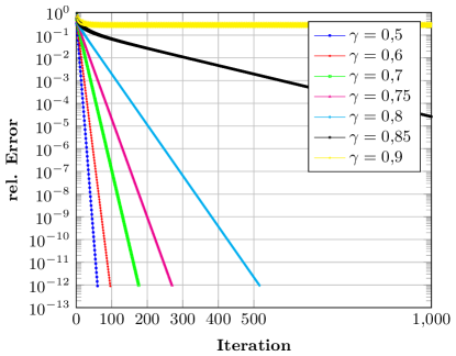
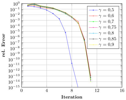
Figure 4.1.1: Convergence results for Simple Kohn-Sham problem by SCF(top), Newton with GMRES (left) and Global GMRES (right)

4.1.2. A 3D model

For our second experiment, we consider (22) with parameters equivalent to those in [14, Sec. 6], where $L$ is a discrete 3D-Laplacian and $\gamma=1$. That is, we have

$$L=L_{m}\otimes I_{m^{2}}+I_{m}\otimes L_{m}\otimes I_{m}+I_{m^{2}}\otimes L_{m},\quad m=\sqrt[3]{n},$$

with $L_{m}=\mathrm{tridiag}(-1,2,-1)\in\mathbb{R}^{m,m}$ being a discrete 1D-Laplacian. We start the SCF-algorithm with $V_{0}\in\mathrm{O}_{n,k}(\mathbb{R})$ being the eigenvectors of $L$ associated with the $k$ smallest eigenvalues and preprocess the Newton algorithm by 50 steps of SCF or until a tolerance of $5\cdot 10^{-5}$ is reached. The Krylov size in both GMRES and GL-GMRES is limited to 400 and $\tau=10^{-10}$ is used as convergence tolerance.
Using this general setup, we examine the performance for the two Newton variants and SCF for $n\in\{10^{3},16^{3},32^{3}\}$ and $k\in\{1,2,3,4,10\}$ and summarize the required average Krylov subspace space size for Newton’s method in Table 4.1.1.

$n$	$\gamma$	$10^{3}$					$16^{3}$					$32^{3}$
$k$		1	2	3	4	10	1	2	3	4	10	1	2	3	4	10
$\varnothing$ Krylov size	1	18.5	26.3	32.7	39	61	26	36.7	40.6	45.5	74	15.1	48.8	25.5	25.3	62.8
	2	18	25.3	28.3	27	54	32.3	32	36.3	56	106	29.1	31.2	46.1	24.6	28.4

Table 4.1.1: Average Krylov subspace size for different problems

In all cases, the average Krylov size required is way smaller than the original problem size, most of the time around $1\%$ of the problem size $n+k$ or even less.
In Figure 4.1.2, we display the convergence results for $n=32^{3}$, $k=2$ and $\gamma=1$. One can see how the quadratic order of convergence leads to convergence after less than 10 steps when switching from SCF to Newton’s method after 22 steps where SCF requires another 80 steps to reach the tolerance. On the right hand side, one can see that GMRES and global GMRES require less than 60 steps for solving the Newton correction equation, which is around $0.2\%$ of the problem size $n+k$, and the time required to do so.

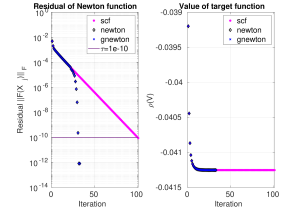
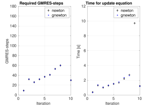
Figure 4.1.2: Convergence results for KS-problem, $n=32^{3}$, $k=2$, $\gamma=1$

4.2. The robust LDA GNEPv

For our next experiment, we consider the GNEPv

$$H(v)v=\lambda G(v)v$$ (26)

originating from robust Rayleigh quotient optimization (RRQM), where the the goal is to find a vector $v\in\mathbb{R}^{n}\setminus\{0\}$ minimizing the Rayleigh quotient

$$r(v)=\frac{v^{T}H(v)v}{v^{T}G(v)v}.$$

Finding robust solutions can be interpreted as optimizing an uncertain, data-based problem for the worst possible behaviour of the input data [4].
In our experiment, we discuss a robust LDA-problem, where we try to find the Fisher discriminant vector $v$ in a two set classification problem. If $X,Y\in\mathbb{R}^{n}$ are two random variables with mean $\mu_{X},\mu_{Y}$ and covariance matrices $\Sigma_{X},\Sigma_{Y}$, it is easy to see that the discriminant vector $v^{*}$ leading to an optimal separation can, up to a scale factor, be uniquely determined by

$$v^{*}=(\Sigma_{X}+\Sigma_{Y})^{-1}(\mu_{Y}-\mu_{Y}).$$ (27)

However, in real life problems, one has usually access to a sample of data only and the sample means and covariances are empirically estimated rather than known explicitly. That is, we have uncertainty in the problem parameters and try to optimize for the worst case behaviour.
In [4, Ex. 5], the following problem is considered: Let

$$H(v)\equiv\overline{\Sigma}_{X}+\overline{\Sigma}_{Y}+(\delta_{X}+\delta_{Y})I_{n}\quad\text{and}\quad G(v)=f(v)f(v)^{T},$$

where

$$f(v)=(\overline{\mu}_{X}-\overline{\mu}_{Y})-\mathrm{sign}\left(v^{T}(\overline{\mu}_{X}-\overline{\mu}_{Y})\right)\left(\frac{S_{X}v}{\sqrt{v^{T}S_{X}v}}+\frac{S_{Y}v}{\sqrt{v^{T}S_{Y}v}}\right).$$ (28)

Here, $\overline{\mu}_{X},\overline{\mu}_{Y}$ and $\overline{\Sigma}_{X},\overline{\Sigma}_{Y}$ are the estimated sample means and covariance matrices, respectively. They are estimated by randomly sampling the data 100 times and computing the average of all 100 computed sample means and covariances. The parameters $\delta_{X},\delta_{Y}$ describe the maximum deviation to the average covariance matrices, that is

$$\delta_{X}=\max_{i=1,...,100}\lVert\overline{\Sigma}_{X}-\Sigma_{X}^{(i)}\rVert_{F},$$

where $\Sigma_{X}^{(i)}$ is the sample covariance matrix in the $i$-th resampling iteration. Similarly, the covariance matrices of the sampled mean values $\mu_{X}^{(i)},\mu_{Y}^{(i)}$ are used to compute $S_{X}$ and $S_{Y}$.
Note than in this application, the Fréchet derivative of $G$ has the special low-rank structure

$$L_{G}(v,e)=f(v)L_{f}(v,e)^{T}+L_{f}(v,e)f(v)^{T},$$

meaning that we do not want to compute the full size matrix explicitly and use scalar products with $f(v)$ and $L_{f}(v,e)$ intstead. The Fréchet derivative of $f(v)$ can be assambled from the Fréchet derivatives of the quotients $q_{S}(v)=\frac{Sv}{\sqrt{v^{T}Sv}}$, which is given by

$$L_{q_{S}}(v,e)=S\left(\frac{1}{\sqrt{v^{T}Sv}}e-\frac{v^{T}Se}{\sqrt{(v^{T}Sv)^{3}}}v\right).$$

Note that $\mathrm{sign}(x)$ is only differentiable with $\mathrm{sign}^{\prime}(x)=0$ if $x\neq 0$, so we require $v$ to not be orthogonal to the difference in sample means for $f$ to be differentiable. In that case, we have

$$L_{f}(v,e)=-\mathrm{sign}\left(v^{T}(\overline{\mu}_{X}-\overline{\mu}_{Y})\right)\left(L_{q_{S_{X}}}(v,e)+L_{q_{S_{Y}}}(v,e)\right).$$

In our experiment, we compare the performance of our algorithm to the two different SCF-algorithms provided by Bai, Lu and Vandereycken in the RobustRQ software package, which is available from http://www.unige.ch/~dlu/rbstrq.html. Their level-shifted SCF-algorithm of order one is denoted by SCF in our plots while their second order SCF-algorithm, which converges quadratically, is denoted by SCF2. Additionally, we compare the classification accuracy to the non-robust LDA solution using the same estimated mean and covariances in (27).
To set up the classification, we split the data into training- and test-data, where the training-data is used to estimate the problem parameters $\overline{\Sigma}$, $\overline{\mu}$, $S$ and $\delta$ and the test-data is used to verify the classification accuracy on unknown data. The amount of training points used is controlled by a parameter $\alpha\in(0,1)$. For every choice of $\alpha$, we perform 100 tests with the data being split randomly every time and plot the average test sample accuracy (TSA) and its deviation.
We verify the performance of our algorithm on two benchmark problems from the UCI machine learning repository [11]: The ionosphere data set, which consists of 351 instances with 34 attributes each, and the sonar data set, which consists of of 208 instances with 60 attributes each. Thus, the corresponding GNEPv will be of size $n=34$ and $n=60$, respectively. Since $k=1$, we use the build-in GMRES for our experiments.
For the ionosphere set, we use $\alpha\in\{0.1,0.15,0.2,0.4,0.6,0.7\}$ for the data splitting and preprocess by 100 steps of SCF and 2 steps of SCF2 or until a tolerance of $10^{-3}$ is reached and switch to Newton’s method afterwards. Here, we allow a Krylov space of size 20 and use $\tau=10^{-8}$ as our convergence tolerance.
In Figure 4.2.1, one can see that the Newton method leads to classifications of comparable accuracy to SCF and SCF2 in a similar computation time. All three approaches are superior to the CLDA in the sense of classification accuracy, justifying the idea to use robust classification. For smaller choices of $\alpha$, Newton’s method is faster than SCF but slower than SCF2, while for $\alpha>0.4$, it is faster than SCF2 but slower than SCF.

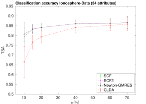
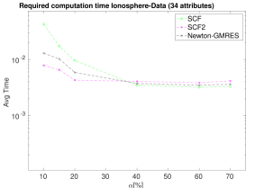
Figure 4.2.1: Convergence results for different choices of $\alpha$, Ionosphere-Data-Set

For the sonar data set, we use $\alpha\in\{0.3,0.4,0.5,0.6,0.7,0.8\}$ and preprocess by 60 steps of SCF and 6 steps of SCF or until a tolerance of $10^{-3}$ is reached. Again, we allow 20 GMRES-steps and use $\tau=10^{-8}$. In Figure 4.2.2, one can observe that the TSA of Newton’s method is able to match SCF and SCF2 while all three robust methods outperform the CLDA. In terms of computation time, our algorithm is faster than SCF but slower than SCF2 for $\alpha\leq 0.5$ and marginally faster than both algorithms for $\alpha\geq 0.6$.
Overall, we can conclude that the Newton algorithm is able to outperform or at least match the SCF algorithm for both data sets and all choices of $\alpha$ while being approximately on par with or slightly faster than the SCF2 algorithm for medium and large choices of $\alpha$ in both examples. Thus, our algorithm is able to compete with SCF for this type of (2) as well.

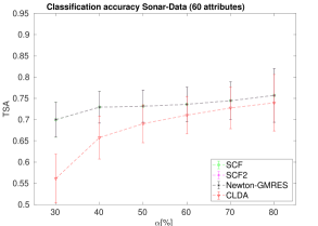
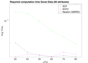
Figure 4.2.2: Convergence results for different choices of $\alpha$, Sonar-Data-Set

4.3. The discrete Gross-Pitaevskii equation

In this last example, we consider a NEPv arising from the discretized Gross-Pitaevskii equation (GPE) [5, 18] in two different variants. The matrix function $H(V)$ is a complex function of the form

$$H(V)=A_{f}+\gamma\mathrm{Diag}(\lvert V\rvert)^{2},$$ (29)

where $A_{f}\in\mathbb{C}^{n,n}$ is Hermitian and positive definite, $\gamma>0$ is a real positive parameter and $\lvert V\rvert$ is the elementwise absolute value of the vector $V\in\mathbb{C}^{n}$.
To have a concrete example, we consider a 2D GPE-model on the domain $\Omega=[-\ell,\ell]\times[-\ell,\ell]$, $l>0$, and a potential function $f:\mathbb{R}^{2}\rightarrow\mathbb{R}$. Then, the matrix $A_{f}$ has the form

$$A_{f}=\mathrm{Diag}(\tilde{f})-\frac{1}{2}M-\mathrm{i}\omega M_{\Phi},$$

where

$$\tilde{f}=h^{2}\left[f(x_{1},y_{1}),f(x_{2},y_{1}),\dots,f(x_{N},y_{1}),f(x_{1},y_{2}),\dots,f(x_{N},y_{2}),\dots,f(x_{N},y_{N})\right]\in\mathbb{R}^{N^{2}}$$

is the discretized potential on the inner mesh points $\{x_{j}\}_{j=1,\dots,N}$, $\{y_{j}\}_{j=1,\dots,N}$ of the uniformly discretized domain $\Omega_{h}$, where $h=\frac{2\ell}{N+1}$, i.e. $x_{j}=y_{j}=-l+j\cdot h$. The matrices $M$ and $M_{\Phi}$ are given by

$$M=D_{2,N}\otimes I_{N}+I_{N}\otimes D_{2,N},\leavevmode\nobreak\ M_{\Phi}=(h\mathrm{Diag}(y_{1},\dots,y_{N}))\otimes D_{N}+D_{N}\otimes(h\mathrm{Diag}(x_{1},\dots,x_{N})),$$

where $D_{N}=\mathrm{tridiag}(-\frac{1}{2},0,\frac{1}{2})$ and $D_{2,N}=\mathrm{tridiag}(1,-2,1)$ are both $N\times N$ real tridiagonal matrices. Note that $M$ is constructed to be symmetric and $M_{\Phi}$ is skew-symmetric since $D_{N}$ is skew-symmetric.
The desired eigenvector $V\in\mathbb{C}^{n}$ is the discretized condensate wave function $\psi(x,y)$ in vectorized form, $\psi(x_{i},y_{j})=V_{N(j-1)+i}$, and $\lvert\psi(x,y)\rvert^{2}$ is proportional to the particle density at $(x,y)$ in the domain.

4.3.1. The complex problem

In the way stated above, NEPv for (29) is a complex problem and, as such, can not be treated by our algorithm from a theoretical point of view since the unitarity constraint is not formally Fréchet differentiable. Nonetheless, we will apply our algorithm to the complex problem and show, that Newton’s method works in the same way for some problems. Since for complex scalars $x,e\in\mathbb{C}$, we have $\lvert x\rvert^{2}=x\overline{x}$, we can see that

$$\lvert x+e\rvert^{2}-\lvert x\rvert^{2}=x\overline{x}+x\overline{e}+\overline{x}e+e\overline{e}-x\overline{x}=\overline{\overline{x}e}+\overline{x}e+\lvert e\rvert^{2}=2\operatorname{Re}(\overline{x}e)+\mathcal{O}(\lvert e\rvert^{2}).$$

Since $A_{f}$ does not depend on $V$, we in consequence have the directional derivative

$$D_{H}(V,E)=2\gamma\mathrm{Diag}\left(\operatorname{Re}(\overline{V}\odot E)\right)$$

taking the formula from above componentwise for $\mathrm{Diag}(\lvert V\rvert)^{2}=\mathrm{Diag}(V\odot\overline{V})$. Note that the directional derivative is again not linear over $\mathbb{C}$ since $\operatorname{Re}(\alpha x)\neq\alpha\operatorname{Re}(x)$, for some $\alpha\in\mathbb{C}$ with $\operatorname{Im}(\alpha)\neq 0$.

4.3.2. A real formulation

In [18], the complex problem (29) was transformed into a real NEPv of doubled size by interpreting the real and imaginary parts of the complex input vector $V=v_{1}+\mathrm{i}v_{2}\in\mathbb{C}^{n}$ as separate variables and writing $\tilde{V}=\begin{bmatrix}v_{1}\\ v_{2}\end{bmatrix}\in\mathbb{R}^{2n}$. For this, (29) was then rewritten in terms of the real matrix function $\tilde{H}:\mathbb{R}^{2n}\rightarrow\mathbb{R}^{2n,2n}$, which has the form

$$\tilde{H}(\tilde{V}) = \begin{bmatrix}\operatorname{Re}(A_{f})&-\operatorname{Im}(A_{f})\\ \operatorname{Im}(A_{f})&\operatorname{Re}(A_{f})\end{bmatrix}+\frac{\gamma}{\tilde{V}^{T}\tilde{V}}B(\tilde{V})$$ (30)

$$= \begin{bmatrix}\mathrm{Diag}(\tilde{f})-\frac{1}{2}M&\omega M_{\Phi}\\ -\omega M_{\Phi}&\mathrm{Diag}(\tilde{f})-\frac{1}{2}M\end{bmatrix}+\frac{\gamma}{{\tilde{V}}^{T}\tilde{V}}B(\tilde{V}),$$

where

$$B(\tilde{V})=\begin{bmatrix}\mathrm{Diag}(v_{1})^{2}+\mathrm{Diag}(v_{2})^{2}&\\ &\mathrm{Diag}(v_{1})^{2}+\mathrm{Diag}(v_{2})^{2}\end{bmatrix}.$$

Since $M$ and $B(\tilde{V})$ are symmetric and $M_{\Phi}$ is skew-symmetric, $\tilde{H}(\tilde{V})$ is symmetric for every $\tilde{V}$. Here, we always have the Fréchet derivative

$$L_{\tilde{H}}(\tilde{V},\tilde{E})=\frac{\gamma}{{\tilde{V}}^{T}\tilde{V}}L_{B}(\tilde{V},\tilde{B})-\frac{2\gamma{\tilde{V}}^{T}\tilde{E}}{({\tilde{V}}^{T}\tilde{V})^{2}}B(\tilde{V}),$$

where

$$L_{B}(\tilde{V},\tilde{E})=\begin{bmatrix}2\mathrm{Diag}(v_{1}\odot e_{1}+v_{2}\odot e_{2})&\\ &2\mathrm{Diag}(v_{1}\odot e_{1}+v_{2}\odot e_{2})\end{bmatrix}$$

and $\tilde{E}=\begin{bmatrix}e_{1}\\ e_{2}\end{bmatrix}$ is split according to the sizes of $v_{1}$ and $v_{2}$. Note that $L_{\tilde{H}}(\tilde{V},\tilde{E})$ is again a diagonal matrix and, as such, can be applied efficiently in the GMRES process.

4.3.3. Numerical results

For our test, we use the setup from [3, Ex. 6.3], where $\Omega=[-1,1]^{2}$, $\omega=0.85$, $N=10$ and $f=\frac{1}{2}(x^{2}+y^{2})$ is a harmonic potential. In this experiment, we again try to investigate the influence of the factor $\gamma$ controlling the problem nonlinearity on the convergence of different methods (see Chapter 4.1.1). The parameter is chosen from a subset of $[0.1,3.5]$, namely $\gamma\in\{0.1,1.0,1.5,2.2,2.6,3.0,3.5\}$ and we compare the performance of Newton’s method and SCF on both the complex problem (29) and the real formulation (30). In our experiment, we are interested in finding the solution associated with the smallest eigenvalue, which is the ground state of the physical system. We use $\tau=10^{-10}$ as a convergence tolerance and switch to Newton’s method after four steps of SCF or whenever the residual is below $10^{-3}$.
In Figure 4.3.1, one can see the convergence behaviour of the four methods as $\gamma$ increases. Similar to the observations from Figure 4.1.1, increasing $\gamma$ leads to a significantly higher amount of iterations required by SCF to find a solution while Newton’s method is less affected by the choice of $\gamma$.

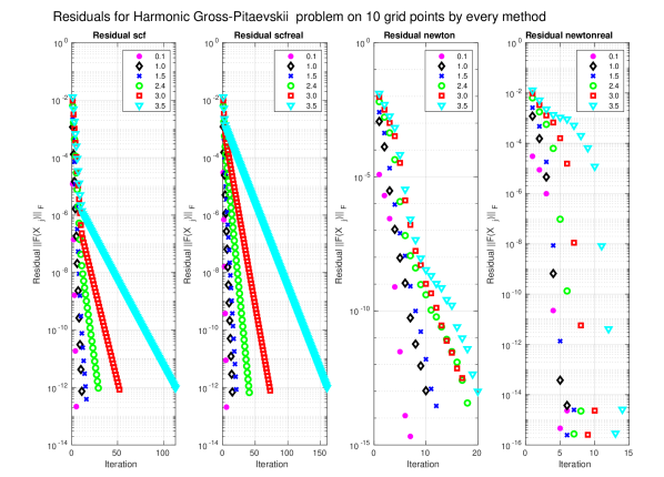
Figure 4.3.1: Convergence results for different methods and different choices of $\gamma$

Notably, the real problem requires more SCF iterations than the equivalent complex problem in most cases, particularly as $\gamma$ gets larger. On the other hand, Newton’s method requires a few more steps for the complex problem as $\gamma$ increases but still converges to a physically equivalent solution, which we can see in Figure 4.3.2. Here, we display the particle density $\lvert\psi(x,y)\rvert^{2}$ for both the original and the real problem for $\gamma=3.5$ computed by Newton’s method on the discrete grid with ten mesh points in every direction as well as the difference in both solutions. One can see that the density is highest in the origin $(0,0)$ and close to zero on the boundary of the domain. Additionally, we observe that the real and complex problem yield a solution that is equal up to an error of order $10^{-14}$ on the entire domain, indicating that our Newton approach can work for complex problems in a similar way.

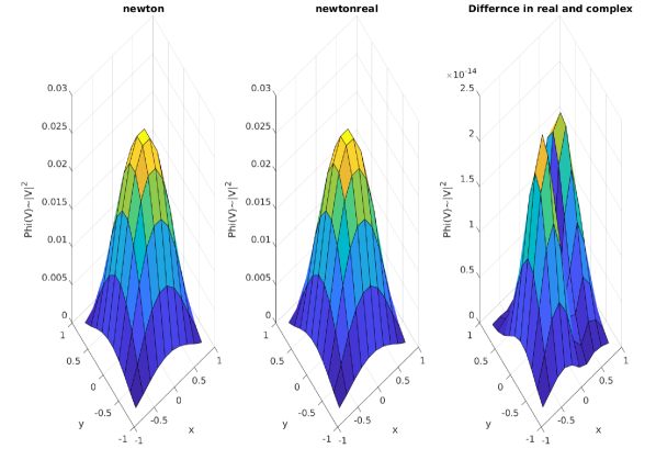
Figure 4.3.2: Solution computed by Newton for (29) and (30)

5. Conclusion

In this paper, we have introduced the inexact Matrix-Newton method for solving NEPv and GNEPv. For this algorithm, we have reported on how to implement the algorithm efficiently by using a global GMRES approach for solving the update equation. The algorithm is then compared to the SCF algorithm in a variety of numerical experiments using MATLAB. Here we could see that the Newton algorithm is able to compete with SCF in most applications where SCF has linear convergence speed and yield optimal solutions, even in some cases where SCF did not converge.
Some future research can be put into employing restarting strategies, such as deflation, to be able to compete if many GL-GMRES steps are necessary. The effect of preconditioning on our algorithm is also an interesting subject we have to pursue.

Code Availability

Source code supporting this paper is available from https://doi.org/10.5281/zenodo.10124821.

References

- [1] Awad Al-Mohy and Nicholas Higham. The complex step approximation to the Fréchet derivative of a matrix function. Numerical Algorithms, 53, 01 2010.
- [2] Kendall E. Atkinson. An introduction to numerical analysis. John Wiley & Sons, 2 edition, 1989.
- [3] Zhaojun Bai, Ren-Cang Li, and Ding Lu. Optimal Convergence Rate of Self-Consistent Field Iteration for Solving Eigenvector-dependent Nonlinear Eigenvalue Problems, 09 2020.
- [4] Zhaojun Bai, Ding Lu, and Bart Vandereycken. Robust Rayleigh Quotient Minimization and Nonlinear Eigenvalue Problems. SIAM Journal on Scientific Computing, 40(5):A3495–A3522, 2018.
- [5] Weizhu Bao and Qiang Du. Computing the Ground State Solution of Bose–Einstein Condensates by a Normalized Gradient Flow. SIAM Journal on Scientific Computing, 25(5):1674–1697, 2004.
- [6] Robert G. Bartle. Newton’s Method in Banach Spaces. Proceedings of the American Mathematical Society, 6(5):827–831, 1955.
- [7] Aharon Ben-Tal, Laurent El Ghaoui, and Arkadi Nemirovski. Robust Optimization. Princeton University Press, 2009.
- [8] Yunfeng Cai, Lei-Hong Zhang, Zhaojun Bai, and Ren-Cang Li. On an Eigenvector-Dependent Nonlinear Eigenvalue Problem. SIAM Journal on Matrix Analysis and Applications, 39(3):1360–1382, 2018.
- [9] Eric Cancès, Gaspard Kemlin, and Antoine Levitt. Convergence analysis of direct minimization and self-consistent iterations. SIAM Journal on Matrix Analysis and Applications, 42(1):243–274, 2021.
- [10] Ron Dembo, Stanley Eisenstat, and Trond Steihaug. Inexact Newton Methods. SIAM J. Numer. Anal., 19:400–408, 04 1982.
- [11] Dheeru Dua and Casey Graff. UCI Machine Learning Repository. http://archive.ics.uci.edu/ml, 2017.
- [12] Stanley C. Eisenstat and Homer F. Walker. Globally Convergent Inexact Newton Methods. SIAM Journal on Optimization, 4(2):393–422, 1994.
- [13] Stanley C. Eisenstat and Homer F. Walker. Choosing the Forcing Terms in an Inexact Newton Method. SIAM Journal on Scientific Computing, 17(1):16–32, 1996.
- [14] Weiguo Gao, Chao Yang, and Juan Meza. Solving a Class of Nonlinear Eigenvalue Problems by Newton’s Method. 11 2009.
- [15] Luc Giraud, Julien Langou, Miroslav Rozlozník, and Jasper van den Eshof. Rounding error analysis of the classical Gram-Schmidt orthogonalization process. Numerische Mathematik, 101:87–100, 2005.
- [16] Nicholas J. Higham. Computing the Polar Decomposition—with Applications. SIAM Journal on Scientific and Statistical Computing, 7(4):1160–1174, 1986.
- [17] Nicholas J. Higham. Functions of Matrices. Society for Industrial and Applied Mathematics, 2008.
- [18] Elias Jarlebring, Simen Kvaal, and Wim Michiels. An Inverse Iteration Method for Eigenvalue Problems with Eigenvector Nonlinearities. SIAM Journal on Scientific Computing, 36(4):A1978–A2001, 2014.
- [19] Khalide Jbilou, Abderrahim Messaoudi, and Hassane Sadok. Global FOM and GMRES algorithms for matrix equations. Applied Numerical Mathematics, 31(1):49–63, 1999.
- [20] Leonid V. Kantorovich and Gleb P. Akilov. Functional Analysis. Pergamon, 2 edition, 1982.
- [21] Dana A. Knoll and David E. Keyes. Jacobian-free Newton–Krylov methods: a survey of approaches and applications. Journal of Computational Physics, 193(2):357–397, 2004.
- [22] Ding Lu. Nonlinear Eigenvector Methods for Convex Minimization over the Numerical Range. SIAM Journal on Matrix Analysis and Applications, 41(4):1771–1796, 2020.
- [23] Richard M. Martin. Electronic Structure: Basic Theory and Practical Methods. Cambridge University Press, Cambridge, 2004.
- [24] Thanh T. Ngo, Mohammed Bellalij, and Yousef Saad. The Trace Ratio Optimization Problem for Dimensionality Reduction. SIAM Journal on Matrix Analysis and Applications, 31(5):2950–2971, 2010.
- [25] Christopher C. Paige, Miroslav Rozlozník, and Zdenvek Strakos. Modified Gram-Schmidt (MGS), Least Squares, and Backward Stability of MGS-GMRES. SIAM Journal on Matrix Analysis and Applications, 28(1):264–284, 2006.
- [26] Yousef Saad, James Chelikowsky, and Suzanne Shontz. Numerical Methods for Electronic Structure Calculations of Materials. SIAM Review, 52:3–54, 03 2010.
- [27] Victor R. Saunders and Ian H. Hillier. A “Level–Shifting” method for converging closed shell Hartree–Fock wave functions. International Journal of Quantum Chemistry, 7(4):699–705, 1973.
- [28] Lea Thøgersen, Jeppe Olsen, Danny Yeager, Poul Jørgensen, Pawel Sałek, and Trygve Helgaker. The trust-region self-consistent field method: Towards a black-box optimization in Hartree-Fock and Kohn-Sham theories. The Journal of chemical physics, 121:16–27, 08 2004.
- [29] Chao Yang, Juan Meza, and Lin-Wang Wang. A Trust Region Direct Constrained Minimization Algorithm for the Kohn–Sham Equation. SIAM J. Scientific Computing, 29:1854–1875, 01 2007.
- [30] Lei-Hong Zhang, Wei Hong Yang, and Li-Zhi Liao. A note on the trace quotient problem. Optimization Letters, 8:1637–1645, 06 2014.