Plug-In RIS: A Novel Approach to Fully Passive Reconfigurable Intelligent Surfaces

Abstract

This paper presents a promising design concept for reconfigurable intelligent surfaces (RISs), named plug-in RIS, wherein the RIS is plugged into an appropriate position in the environment, adjusted once according to the location of both base station and blocked region, and operates with fixed beams to enhance the system performance. The plug-in RIS is a novel system design, streamlining RIS-assisted millimeter-wave (mmWave) communication without requiring decoupling two parts of the end-to-end channel, traditional control signal transmission, and online RIS configuration. In plug-in RIS-aided transmission, the transmitter efficiently activates specific regions of the divided large RIS by employing hybrid beamforming techniques, each with predetermined phase adjustments tailored to reflect signals to desired user locations. This user-centric approach enhances connectivity and overall user experience by dynamically illuminating the targeted user based on location. By introducing plug-in RIS’s theoretical framework, design principles, and performance evaluation, we demonstrate its potential to revolutionize mmWave communications in limited channel state information (CSI) scenarios. Simulation results illustrate that plug-in RIS provides power/cost-efficient solutions to overcome blockage in the mmWave communication system and a striking convergence in average bit error rate and achievable rate performance with traditional full CSI-enabled RIS solutions.

I Introduction

The requirements posed by the next generation of communication networks, including massive connectivity, ultra-reliability, low latency, and energy efficiency, necessitate exploring innovative strategies and technologies to enhance existing communication systems, enabling the deployment of ubiquitous connected devices. Reconfigurable intelligent surfaces (RISs), a promising technology that acquired substantial attention from research community, has emerged as a potential candidate for incorporation into the next-generation wireless communication networks [1]. By intelligently manipulating incident signals, RISs enable a smart environment through controlled scattering paths, significantly improving performance. The RIS-aided virtual channel between the terminals, making the channel adaptable for boosting communication performance in various scenarios or circumventing blockages that impede communication, a common occurrence in millimeter-wave (mmWave) communication systems due to signal vulnerability to the blockage and severe path loss. These blocked regions, termed dead zones, can be addressed by properly configuring the RIS phase shifts based on channel state information (CSI), allowing the RIS to redirect signals around obstructions and serve users within the dead zones. It is worth mentioning that CSI acquisition and phase shift configuration are key limiting factors significantly affecting the RIS design and system performance. Hence, the following sub-section elaborates on different RIS designs in the existing literature, mostly focusing on CSI acquisition methods for RIS phase adjustment [2, 3, 4, 5, 6, 7, 8, 9, 10, 11, 12].

TABLE I: Comparison among different RIS structures available in the existing literature and the proposed plug-in RIS.
(Abbreviations: Y = yes; N = no; FP = fully passive; SP = semi-passive; H = high; M = medium; L = low.)

[2]

[3]

[4]

[5]

[6]

[7]

[8]

[9]

[10]

[11]

[12]

Plug-in RIS

RIS type:

FP

FP

FP

FP

FP

FP

FP

SP

SP

SP

SP

FP

Channel estimation carries out by:

BS

UE

BS

UE

UE

BS

UE

RIS

RIS

BS/UE

BS/UE

BS

Control link availability:

Y

Y

Y

Y

Y

Y

Y

N

N

Y

Y

N

Implementation complexity:

M

M

H

H

H

M

H

H

H

M

M

L

Signalling overhead:

M

M

H

M

M

M

H

L

L

M

M

L

I-A Related Works

Two critical aspects distinguishing RIS deployment are its passive nature and ease of implementation, as highlighted in [1]. Specifically, it is assumed that an ideal RIS does not require an external power source and can be easily adapted for implementation in various environments. By taking these attributes into account, we classify the existing RIS structures into two main categories: Fully passive RIS and semi-passive RIS.

I-A1 Fully passive RIS

The RIS configuration depends on CSI availability for both the base station (BS)-RIS and RIS-user equipment (UE) channels, as assumed in most RIS studies in the literature. In a fully passive RIS setup, where the RIS lacks baseband processing capability, either the BS or the UE needs to estimate the end-to-end channel and decouple two parts of it, i.e., BS-RIS and RIS-UE. Numerous studies in the existing literature have addressed the channel estimation problem for fully passive RIS systems [2, 3, 4, 5, 6, 7, 8].

In [2], the authors proposed a channel estimation method for passive RIS-assisted energy transfer systems, assuming that the power beacon manages all computational tasks due to constraints in UE. In [3], the authors studied channel estimation in an RIS-assisted mmWave communication system, aiming for joint active and passive beamforming for single-antenna UEs; nevertheless, dealing with multi-antenna UEs adds extra computational load for CSI acquisition and passive phase shift vector optimization. The study of [4] proposed a two-step channel estimation protocol for acquiring two parts of the end-to-end channel within a multi-user (MU) mmWave MIMO system, in which the BS is responsible for channel estimation. Meanwhile, the study of [5] dives into channel estimation problem within a point-to-point (P2P) RIS-assisted mmWave communication system. Under the suggested protocol, the UE undertakes an optimization problem to obtain downlink cascaded channels. Similarly, a channel estimation algorithm for passive large intelligent metasurfaces (LIM) is introduced in [6], employing sparse matrix factorization and matrix completion. In [7], the authors considered UE mobility and proposed a two-time scale channel estimation framework, leveraging the quasi-static BS-RIS channel while the RIS-UE is a low-dimensional mobile channel. The study of [8] investigated channel estimation for broadband RIS-aided mmWave massive MIMO systems utilizing compressive sensing (CS) method.

This literature review reveals that significant efforts have been made to estimate the end-to-end channel and separate it into BS-RIS and RIS-UE components in RIS-assisted mmWave communication systems. It is worth emphasizing that in fully passive RIS design, channel estimation/decoupling and optimizing phase shifts are done at one of the endpoints, which necessitates two key considerations. Firstly, establishing a dedicated control link is essential to facilitate the transmission of configuration information from the responsible endpoint to the RIS. Secondly, allocating sufficient resources to accommodate the computational tasks associated with channel estimation/decoupling and RIS phase shift optimization at the responsible endpoint is essential. However, it is worth noting that both of these requirements have potential drawbacks. Introducing a dedicated control link can add complexity to the system and potentially increase the overall latency stemming from reconfiguration latency [14], while allocating substantial resources, particularly at the UE, may not be a cost/power-efficient solution. Similarly, if the BS assumes the responsibility for computational tasks, extending this approach to an MU scenario can significantly elevate system complexity and overhead, potentially posing challenges to the overall feasibility of the system.

I-A2 Semi-passive RIS

Despite extensive endeavors to acquire individual cascaded channels for fully passive RIS configurations, challenges arise from the inefficient cascaded channel decoupling process due to the passive nature of RIS elements [9]. In order to address this issue, semi-passive RIS structure is introduced in [10]. In the semi-passive RIS design, a fraction of RIS elements are connected to baseband components, enabling the RIS to perform channel estimation through its integrated baseband components. Consequently, the RIS can accurately estimate BS-RIS and RIS-UE channels separately and adjust itself without being controlled by other terminals, i.e., the transmitter (Tx) or the receiver (Rx) [10]. In [9], the authors proposed an algorithm for semi-passive RIS channel estimation, leveraging sparsity in both spatial and frequency domains of mmWave channels. As shown in [9], connecting only $8\%$ of RIS elements to the baseband components yields more accurate channel estimation than the considered benchmarks. The study of [11] proposed two practical residual neural networks to accurately estimate the channel for semi-passive RIS-aided communication systems. Similarly, the authors in [12] proposed a channel estimation method for semi-passive RIS-assisted systems based on super-resolution neural networks. It is worth noting that even though the studies of [11, 12] exploit semi-passive RIS, a significant portion of the computational load for channel estimation is carried out by the transceivers to simplify the RIS structure. Consequently, they inherit some of the drawbacks associated with both fully passive and semi-passive RIS designs.

Table I provides an overview of the structural characteristics of various RIS designs discussed above. A notable potential advantage of the semi-passive RIS design is its reduced reliance on establishing a dedicated control link. Moreover, this approach eliminates the additional overhead and complexity imposed on the transceivers, as the RIS efficiently handles the computational tasks. Nonetheless, the semi-passive RIS configuration deviates from two fundamental characteristics highlighted previously: The passive nature of the RIS and its simplicity of implementation. While it is evident that the semi-passive RIS does not adhere to the passive attribute, it is crucial to remember that including baseband components introduces a costly and power-intensive structure, which, in turn, hinders easy and widespread deployment.

I-B Motivations and contributions

As summarized in Table I, both fully passive and semi-passive RIS configurations exhibit drawbacks that pose challenges to their practical implementation. Based on the existing literature, it becomes evident that there is a clear and pressing need within academia to create a novel RIS structure that fulfills the two fundamental attributes emphasized in [1], which strongly motivates us to introduce a fresh and innovative design, named plug-in RIS, with the specific aim of simplified deployment and operation within mmWave communication environments. In this system, the RIS can be conveniently plugged into the environment to operate with fixed phase shift profiles, which are adjusted based on the location of the BS and dead zones. Specifically, initially, the dead zone in the mmWave environment is defined to the BS (because the BS is initially not aware of which area is the dead zone) and divided into spatial segments; each spatial segment is considered to be served via a part of divided RIS, named sub-RIS. Next, we examine the location of each spatial segment and assign a fixed phase shift profile to the corresponding sub-RIS. Since both the BS and dead zone have fixed locations, the sub-RISs are not required to be configured frequently. For activation, the BS obtains the UE’s spatial segment and employs beamforming techniques to illuminate the corresponding sub-RIS, enabling control over signal reflection towards desired directions and offering a user-centric approach to enhance wireless communication performance.

Based on the aforementioned motivations, we outline our contributions as follows:

• Plug-in RIS with standalone operation: In contrast to the fully passive and semi-passive RIS designs, this study introduces an innovative approach—a plug-in RIS configuration with standalone operation—for extending communication coverage in mmWave systems. The proposed structure aligns with key attributes of RIS technology, such as, its passive nature and ease of implementation. The plug-in RIS consists of multiple sub-RIS planes, each pre-configured with fixed phase shifts, intended to cover distinct spatial segments within the dead zone. Leveraging the high beamforming gain at the Tx in the mmWave communication systems, only one sub-RIS plane is activated in each transmission period to establish a virtual link toward the UE. This approach innovatively integrates the control mechanism within the transmitting beam, eliminating the necessity for implementing traditional control links and the associated overheads, which enhances the overall user experience by increasing the ease of implementation of the RIS in different environments.

• Compatibility with existing end-to-end channel estimation methods: The pre-configured phase shift design of the suggested plug-in RIS eliminates the necessity for decoupling two parts of the end-to-end channel, which alleviates the additional burden of channel decoupling on the participating terminals, enabling the easy deployment of fully passive RIS in mmWave communication systems. In other words, in the proposed plug-in RIS, obtaining the conventional end-to-end channel estimation is enough, and decoupling it into BS-RIS and RIS-UE channels is not required.

• Reliability analysis: We derive a closed-form expression for the upper bound of the average bit error rate (ABER) for the proposed plug-in RIS. Our analytical methodology employs the union-bound and pairwise error probability (PEP) to validate the precision of our simulation outcomes. Our results illustrate that these analytical derivations offer a tight upper bound on the ABER.

• Simulation insights: We conduct exhaustive simulations to evaluate the performance of the proposed plug-in RIS in terms of ABER, achievable rate, energy efficiency, and detector complexity. Computer simulation outcomes indicate that the plug-in RIS exhibits promising effectiveness, showing close ABER and achievable rate results to the semi-passive design. Moreover, the plug-in RIS outperforms the benchmark designs in terms of energy efficiency and detector complexity, highlighting the superiority of our proposed approach, taking a step forward to the practical implementation of fully passive RIS.

The rest of this article is organized as follows. Section II outlines the system, channel, and signal models. The design of the proposed plug-in RIS is elaborated in Section III. Analytical expression as an upper bound for ABER performance is derived in Section IV. Simulation results are displayed in Section V, followed by the conclusion of this study in Section VI.

Notation: In this paper, bold lowercase and uppercase letters denote column vectors and matrices, respectively. The symbols $(.)^{H}$, $(.)^{T}$, $(.)^{*}$ $|.|$, $||.||$, and $\operatorname*{diag}(.)$ stand for Hermitian, transpose, conjugate, absolute value, norm, and diagonalization, respectively. The operator $\mathbb{E}[.]$ shows the expected value, $\mathcal{R}(.)$ denotes the real component of a complex number, and operator $\circ$ represents the Hadamard (element-wise) product. The notation $\mathcal{CN}(\mu,\sigma^{2})$ represents the complex Gaussian distribution with mean $\mu$ and variance $\sigma^{2}$, while $\mathcal{N}(\mu,\sigma^{2})$ denotes the Gaussian distribution with mean $\mu$ and variance $\sigma^{2}$. The identity matrix of dimension $n$ is represented as $\mathbf{I}_{n}$, while the vector comprising all zeros and ones of size $n$ is denoted by $\mathbf{0}_{n}$ and $\mathbf{1}_{n}$, respectively. Additionally, $\mathcal{U}(a,b)$ indicates a uniform distribution parameterized by $a$ and $b$. The $Q$-function is denoted and defines as $Q(x)=\frac{1}{\sqrt{2\pi}}\int_{x}^{\infty}\exp{(-\frac{u^{2}}{2})}du$. It is worth mentioning that in this paper, the variable $i$ is employed as a local variable, and its assigned value within each equation is applicable only to that equation.

II System, Channel, and Signal Model

This section describes the system model for the mmWave massive MIMO communication system aided by the proposed plug-in RIS. Afterward, we present the utilized channel model and the foundational assumptions supporting our suggested design. Lastly, we elaborate on the signal model and introduce a suitable maximum likelihood (ML) detector.

II-A System Model

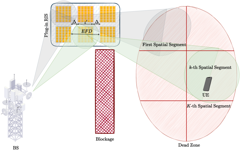
Figure 1: System model for proposed plug-in RIS.

As depicted in Fig. 1, we investigate a P2P mmWave communication system aided by a set of sub-RIS planes with pre-configured fixed phase shifts. Due to propagation loss challenges, the direct BS-UE link is assumed to be blocked, causing dead zones in the environment; therefore, the sub-RIS planes are plugged into the surrounding environment to assist UEs located in the dead zone, ensure constant connectivity and guarantee line-of-sight (LOS) links in the BS-RIS and RIS-UE channels. Specifically, a dead zone can be covered using one or more sub-RISs, each covering a distinct spatial segment of the dead zone with a fixed beam. The set of sub-RISs constitutes the plug-in RIS entity. During implementation, each sub-RIS is assigned to a spatial segment in the dead zone; therefore, they are adjusted according to the angular information of BS and the spatial segments. Specifically, for each spatial segment, we consider fixed angular information that represents it, and since this angular information is constant, the sub-RISs are not required to be adjusted frequently. During the transmission, based on the UE’s location and with the aid of massive MIMO’s beamforming gain at the BS, the transmitted beam footprint only activates the corresponding sub-RIS. Both the BS and UE are equipped with uniform rectangular arrays (URA); $N_{t}$ and $N_{r}$ denote the number of antenna elements at the BS and UE, respectively. To address severe path loss while minimizing the need for costly RF chains, analog beamformers/combiners are employed at the BS/UE. This approach allows a single RF chain at the BS and UE, supporting a single stream [15]. Our proposed plug-in RIS comprises $K$ sub-RISs, each containing $M_{k}\ (k=1,\dots,K)$ passive reflecting elements.

II-B Channel Model

In this paper, we adopt the popular Saleh-Valenzuela (SV) channel model for the BS-RIS and RIS-UE channels as follows [16, 17, 18, 19]:

$$\begin{split}\mathbf{G}_{k}=&\sqrt{N_{t}M_{k}}\alpha_{k}\mathbf{a}_{r,ris}(\varphi_{r,ris}^{k},\vartheta_{r,ris}^{k})\mathbf{a}_{t}^{H}(\varphi_{t},\vartheta_{t}),\end{split}$$ (1)

$$\begin{split}\mathbf{R}_{k}=&\sqrt{M_{k}N_{r}}\beta_{k}\mathbf{a}_{r}(\varphi_{r},\vartheta_{r})\mathbf{a}_{t,ris}^{H}(\varphi_{t,ris}^{k},\vartheta_{t,ris}^{k}),\end{split}$$ (2)

where $\mathbf{G}_{k}\in\mathbb{C}^{M_{k}\times N_{t}}$ ($\mathbf{R}_{k}\in\mathbb{C}^{N_{r}\times M_{k}}$) is the channel between BS and $k$-th sub-RIS ($k$-th sub-RIS and UE). The parameter $\alpha_{k}$ ($\beta_{k}$) is the LOS channel gain of $\mathbf{G}_{k}$ ($\mathbf{R}_{k}$) and follows a complex normal distribution $\mathcal{CN}(0,10^{-0.1PL(d)})$, with $PL(d)$ representing path loss and $d$ indicating the distance between the associated terminals. The array response (steering) vector is denoted as $\mathbf{a}(.)$, while $\varphi\in\mathcal{U}(a_{\varphi},b_{\varphi})$ and $\vartheta\in\mathcal{U}(a_{\vartheta},b_{\vartheta})$ stand for azimuth and elevation angles, respectively. Specifically, $\varphi_{t}$ ($\vartheta_{t}$) represents the azimuth (elevation) angle of departure (AoD) at the BS, and $\varphi_{r}$ ($\vartheta_{r}$) indicates the azimuth (elevation) angle of arrival (AoA) at the UE; this is while, $\varphi_{t,ris}^{k}$ ($\vartheta_{t,ris}^{k}$) shows azimuth (elevation) AoD associated with the $k$-th sub-RIS, and $\varphi_{r,ris}^{k}$ ($\vartheta_{r,ris}^{k}$) is the azimuth (elevation) AoA at the $k$-th sub-RIS. Here, it is assumed that each channel is LOS dominated due to the presence of LOS component [20]. Thus, non-LOS (NLOS) components are omitted, allowing for a focused investigation of the proposed plug-in RIS performance. The normalized antenna array response is defined as follows [15, 20]:

$$\mathbf{a}(\varphi,\vartheta)=\frac{1}{\sqrt{N}}[e^{j\mathbf{k}^{T}\mathbf{p}_{0}},e^{j\mathbf{k}^{T}\mathbf{p}_{1}},\dots,e^{j\mathbf{k}^{T}\mathbf{p}_{N-1}}]^{T},$$ (3)

where $N$ represents the total number of antenna elements/reflectors at the corresponding terminal, calculated as $N=N_{x}\times N_{y}$. Here, $N_{x}$ ($N_{y}$) refers to the number of antenna elements/reflectors along the $x$-axis ($y$-axis). The symbol $\mathbf{k}$ denotes the wave number, and $\mathbf{p}_{n}$ is associated with the structure of the antenna array, specifying the location of the $n$-th antenna element. We establish $n=n_{y}N_{x}+n_{x}$, where $0\leq n_{x}\leq N_{x}-1$ ($0\leq n_{y}\leq N_{y}-1$) represents the location of the antenna element/reflector along the $x$-axis ($y$-axis). For the URA configuration, the definitions of $\mathbf{k}$ and $\mathbf{p}_{n}$ are outlined as follows [15, 20]:

$$\mathbf{k}=\frac{2\pi}{\lambda}[\sin{\vartheta}\cos{\varphi}\enspace\sin{\vartheta}\sin{\varphi}]^{T},$$ (4)

$$\mathbf{p}_{n}=[n_{x}\delta_{x}\enspace n_{y}\delta_{y}]^{T},$$ (5)

where $\delta_{x}$ ($\delta_{y}$) represents the separation between adjacent antennas/reflectors along the $x$-axis ($y$-axis), and $\lambda$ denotes the signal wavelength. Note that to calculate the antenna array response for each terminal, we need to substitute its corresponding $\varphi$ and $\vartheta$ values into (3) and (4). The effective end-to-end channel between the BS and UE through the $k$-th sub-RIS, denoted as $\mathbf{H}_{\text{eff},k}\in\mathbb{C}^{N_{r}\times N_{t}}$, can be defined as follows:

$$\mathbf{H}_{\text{eff},k}=\mathbf{R}_{k}\mathbf{\Psi}_{k}\mathbf{G}_{k},$$ (6)

where $\mathbf{\Psi}_{k}\in\mathbb{C}^{M_{k}\times M_{k}}$ is the $k$-th sub-RIS phase shift matrix and define as

$$\mathbf{\Psi}_{k}\triangleq\operatorname*{diag}{(e^{j\psi_{1}},e^{j\psi_{2}},\dots,e^{j\psi_{M_{k}}})},$$ (7)

where $\psi_{i}$ is the phase shift associated with the $i$-th reflector of the corresponding sub-RIS. As mentioned earlier, the sub-RISs can be adjusted using the location of BS and dead zones. Lemma 1 gives a mathematical expression for sub-RISs phase shift adjustment.

Lemma 1.

The phase shift matrix for the $k$-th sub-RIS can be calculated as follows:

$$\mathbf{\Psi}_{k}=\sqrt{M_{k}}\operatorname*{diag}\Big{(}\mathbf{f}_{b,k}\circ{\mathbf{a}_{r,ris}^{*}}(\varphi_{r,ris}^{k},\vartheta_{r,ris}^{k})\Big{)},$$ (8)

where $\mathbf{f}_{b,k}$ represents the fixed beam formed by the $k$-th sub-RIS with azimuth and elevation AoD as $\phi_{b,k}$ and $\theta_{b,k}$, respectively. $\mathbf{f}_{b,k}$ is expressed as

$$\mathbf{f}_{b,k}=[e^{\mathbf{k}^{T}\mathbf{p}_{0}},e^{\mathbf{k}^{T}\mathbf{p}_{1}},\dots,e^{\mathbf{k}^{T}\mathbf{p}_{M_{k}-1}}],$$

where $\mathbf{k}$ is calculated as (4) by substituting $\varphi=\phi_{b,k}$ and $\vartheta=\theta_{b,k}$.

Proof.

See [18, Section III-C]. ∎

II-C Signal Model

In this subsection, we describe the signal model used in this paper. Next, we represent the ML decoder for the proposed plug-in RIS. As mentioned earlier, the dead zone is divided into distinct spatial segments based on its geometric shape. Given that the dead zone’s location remains fixed, the spatial segments also maintain constant positions. Consequently, each spatial segment is defined by a pair of unchanging azimuth and elevation angular values. Thus, sub-RISs are adjusted according to the constant angular information of BS and spatial segments in order to cover that segment. For starting transmission, the BS should obtain the CSI, including angular information at the BS and UE. Since the BS and sub-RISs have fixed positions, the angular information at the BS is also constant and known to the BS; therefore, after transmitting pilot signals, the BS can easily find the spatial segment in which the UE is located and its associated sub-RIS. Furthermore, by estimating end-to-end channel, both the BS and UE can adjust their analog beamformers/combiners accordingly. The effective end-to-end channel can be described as (6). Therefore, the received signal after passing through the combiner is represented as

$$y=\sqrt{P}G_{t}G_{r}\mathbf{f}_{r}^{H}\mathbf{H}_{\text{eff},k}\mathbf{f}_{t}s+\mathbf{f}_{r}^{H}\mathbf{n},$$ (9)

where $P$ stands for the transmit power, $G_{i}=g_{e}+10\log_{10}(N_{i})$, wherein $i\in\{t,r\}$, represents the array gain, with $g_{e}$ denoting the gain of each antenna element [21, 22]. The symbol $s$ corresponds to the transmitted $\mathcal{M}$-ary symbol, and $\mathbf{n}\in\mathbb{C}^{N_{r}\times 1}\sim\mathcal{C}\mathcal{N}(0,\sigma^{2})$ is the additive noise component. Moreover, $\mathbf{f}_{t}\in\mathbb{C}^{N_{t}\times 1}$ denotes the analog beamformer at the BS, while $\mathbf{f}_{r}\in\mathbb{C}^{N_{r}\times 1}$ represents the analog combiner at the UE. For simplification, continuous phase shifters are assumed at the BS and UE; thus, analog beamformer/combiner can be adjusted as $\mathbf{f}_{t}=\mathbf{a}_{t}(\varphi_{t},\vartheta_{t})$ and $\mathbf{f}_{r}=\mathbf{a}_{r}(\varphi_{r},\vartheta_{r})$. Utilizing the ML detector at the UE, the estimated symbol is expressed as

$$\hat{s}=\operatorname*{arg\,min}_{\forall s\in\mathcal{S}}|y-\sqrt{P}G_{t}G_{r}\mathbf{f}_{r}^{H}\mathbf{H}_{\text{eff},k}\mathbf{f}_{t}s|^{2},$$ (10)

where $\mathcal{S}$ is the set of $\mathcal{M}$-ary constellation points.

III Proposed Plug-in RIS Structure

This section illustrates the structure of the proposed plug-in RIS. In the plug-in RIS structure, sub-RIS units are placed with appropriate spacing, each pre-configured to cover a specific spatial segment within a well-known dead zone. Based on environmental blockage and path loss conditions, the sub-RIS units can be positioned on either the BS or UE side. The spacing between sub-RIS units should increase as they are deployed farther from the BS. We subsequently formulate the minimum spacing between sub-RIS units. Additionally, in Section V, we illustrate the dead zone spatial segments through a graphical example using the simulation setup parameters.

Maintaining an appropriate spacing between sub-RIS units is crucial for reducing power leakage to other segments within the dead zone, which is particularly beneficial in MU scenarios as it leads to decreased interference. Leveraging the beamforming gain offered by the massive MIMO antenna array at the BS, forming a narrow beam precisely directed to a specific spatial area becomes feasible. This beam’s coverage area, termed footprint, is determined by the distance from the BS and the emitted signal’s beamwidth. Exploiting this property of massive MIMO arrays enables the BS to illuminate only the corresponding sub-RIS based on the UE’s location. In Fig. 1, an illustration of adjacent sub-RISs separated by $\Delta$ is shown. To establish a closed-form expression for $\Delta$, we initially define the length of each side of the sub-RIS along the $i$-axis (where $i\in\{x,y\}$) as $\iota_{i}=M_{i}\delta_{i}$. Note that $M_{i}$ represents the number of reflectors across the $i$-axis, and for simplicity in notation, we eliminated the sub-RIS’s index. The footprint of the received beam should exclusively cover the intended sub-RIS. Assuming uniform spacing between sub-RISs, the effective footprint diameter (EFD) can be computed as $\textrm{EFD}=2\Delta+\iota$. Consequently, $\Delta$ can be derived as follows:

$$\Delta=\frac{\textrm{EFD}-\iota}{2}.$$ (11)

In order to determine the EFD, we consider half-power beamwidth (HPBW) that encompasses an effective portion of the radiated power [23]. It is worth mentioning that an antenna can differentiate between two adjacent sources if the angular separation between them exceeds half of the first-null beamwidth (FNBW), which is approximately equivalent to HPBW, i.e., $\textrm{HPBW}\approx\frac{\textrm{FNBW}}{2}$ [24]. The HPBW of an antenna array along the $i$-axis ($i\in\{x,y\}$) can be calculated using the following formula [25]:

$$\textrm{HPBW}\approx 0.891\frac{\lambda}{N_{i}\delta_{i}}.$$ (12)

Lemma 2.

The EFD of the transmitted beam from the Tx at a distance of $d$ can be computed as follows:

$$\textrm{EFD}=2d\times\frac{\sin{(\frac{\textrm{HPBW}}{2})}}{\cos{(\frac{\textrm{HPBW}}{2}+\theta_{0})}},$$ (13)

where $\theta_{0}$ represents the angle of the incident signal at the RIS with respect to the RIS broadside direction.

Proof.

See [26, Appendix B]. ∎

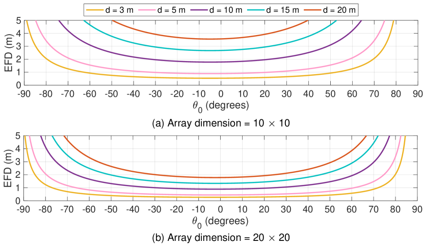
Figure 2: EFD versus different amounts of incident angle.

Corollary 1.

In the case where $\theta_{0}=0$, indicating that the received beam at the RIS is perpendicular to the RIS surface, the EFD can be approximated as

$$\textrm{EFD}\approx\textrm{HPBW}\times d.$$ (14)

Proof.

See Appendix A. ∎

Fig. 2 illustrates the precise EFD for various values of $d$ and $\theta_{0}$. Notably, in Figs. 2 (a) and (b), a distinct pattern emerges: within a limited range centered around $\theta_{0}=0^{\circ}$, the EFD remains constant; the extent of this interval diminishes with higher values of $d$. Conversely, as it is illustrated in Fig 2. (b), adopting a larger antenna array leads to expanding the interval.

Substituting EFD into (11), sub-RISs inter-spacing, i.e., $\Delta$, can be calculated as

$$\Delta=\frac{\textrm{HPBW}\times d-\iota}{2}.$$ (15)

Notably, $\Delta$ defines the minimum distance that needs to be maintained between two neighboring sub-RIS units to mitigate power leakage to the other spatial segments.

IV Theoretical Analysis

In this section, we begin by presenting a mathematical expression to validate the accuracy of our ABER simulation results. Following that, we provide expressions for computing the detector’s complexity for both plug-in and semi-passive RIS designs.

IV-A ABER Theoretical Upper Bound

Obtaining ABER involves calculating the pairwise error probability (PEP), which denotes the likelihood of detecting $\hat{s}$ when transmitting $s^{*}$. Initially, we consider the channel as a known entity for both cascaded channels. This allows us to express the conditional PEP (CPEP) as follows:

$$\begin{split}\mathcal{P}(s^{*}\rightarrow\hat{s}|\alpha_{k},\beta_{k})=&\mathcal{P}(|y-\sqrt{P}G_{t}G_{r}\mathbf{f}_{r}^{H}\mathbf{H}_{\text{eff},k}\mathbf{f}_{t}s^{*}|^{2}\\ &>|y-\sqrt{P}G_{t}G_{r}\mathbf{f}_{r}^{H}\mathbf{H}_{\text{eff},k}\mathbf{f}_{t}\hat{s}|^{2}).\end{split}$$ (16)

Lemma 3.

The mathematical expression for CPEP is as

$$\begin{split}\mathcal{P}(s^{*}\rightarrow&\hat{s}|\alpha_{k},\beta_{k})\\ &=Q\Big{(}\frac{\sqrt{P}G_{t}G_{r}|\mathbf{f}_{r}^{H}\mathbf{H}_{\text{eff},k}\mathbf{f}_{t}(s^{*}-\hat{s})|^{2}}{\sqrt{2}\sigma||\mathbf{f}_{r}\mathbf{f}_{r}^{H}\mathbf{H}_{\text{eff},k}\mathbf{f}_{t}(s^{*}-\hat{s})||}\Big{)}.\end{split}$$ (17)

Proof.

See Appendix B. ∎

Lemma 3 provides a closed-form expression for the CPEP. To compute the unconditional PEP (UPEP), we take the expectation of CPEP over a sufficient number of channel realizations, denoted as $\mathrm{UPEP}=\mathbb{E}[\mathrm{CPEP}]$. Furthermore, to establish an upper bound for the ABER, we utilize the union-bound approach as follows:

$$\textrm{ABER}\leq\frac{1}{\eta\mathcal{M}}\sum_{s^{*}}\sum_{\hat{s}}E_{b}(s^{*}\rightarrow\hat{s})\textrm{UPEP},$$ (18)

where $E_{b}(s^{*}\rightarrow\hat{s})$ is the total number of erroneous bits and $\mathcal{M}$ is the order of $\mathcal{M}$-ary constellation.

IV-B Detector Complexity

This subsection discusses the computation of detector complexity for our suggested plug-in RIS and semi-passive RIS designs. Both designs employ the same detector as given in (10), but the main difference lies in obtaining $\mathbf{H}_{\text{eff}}$. In the semi-passive RIS design, $\mathbf{G}$ and $\mathbf{R}$ are computed separately, and the phase shift matrix $\mathbf{\Psi}$ is also calculated by the RIS in each transmission period. The detector then uses these matrices to calculate $\mathbf{H}_{\text{eff}}$, affecting the detector’s complexity. However, in the plug-in RIS design, $\mathbf{H}_{\text{eff}}$ is directly acquired without the need for separate calculations of $\mathbf{G}$, $\mathbf{R}$, and $\mathbf{\Psi}$ due to the pre-adjusted sub-RIS configuration. Considering this point, we compute each RIS systems’s detector complexity as follows. In this subsection, for the sake of notation simplicity, we show the number of RIS/sub-RIS elements engaged in the communication with $M$; hence, the index of sub-RISs has been ignored.

1. Semi-passive RIS: To compute $\mathbf{H}_{\text{eff}}$, the detector calculates $\mathbf{\Psi}\mathbf{G}$, involving $\sim M^{2}N_{t}$ operations. Subsequently, $\mathbf{R}\mathbf{\Psi}\mathbf{G}$ demands $\sim N_{r}MN_{t}$ operations. Thus, for computing $\mathbf{H}_{\text{eff}}$, $\sim M^{2}N_{t}+N_{r}MN_{t}$ operations are needed. Moreover, $\mathbf{H}_{\text{eff}}\mathbf{f}_{t}$ entails $\sim N_{r}N_{t}$ operations, and obtaining $\mathbf{f}_{r}^{H}\mathbf{H}_{\text{eff}}\mathbf{f}_{t}$ takes $\sim N_{r}$ operations. With this procedure repeated $\mathcal{M}$ times, the detector’s complexity is $\mathcal{O}(\mathcal{M}(M^{2}N_{t}+N_{r}MN_{t}+N_{t}N_{r}+N_{r}))$. However, by neglecting the lower-order terms $N_{t}N_{r}+N_{r}$, the complexity of the semi-passive RIS detector can be simplified to $\sim\mathcal{O}(\mathcal{M}MN_{t}(M+N_{r}))$.

2. Plug-in RIS: In the plug-in RIS design, the detector has direct access to $\mathbf{H}_{\text{eff}}$ as explained earlier. Thus, in the initial step, it computes $\mathbf{H}_{\text{eff}}\mathbf{f}_{t}$, requiring $\sim N_{r}N_{t}$ operations. Following this, to calculate $\mathbf{f}_{r}^{H}\mathbf{H}_{\text{eff}}\mathbf{f}_{t}$, the detector performs $\sim N_{r}$ operations. This process is repeated $\mathcal{M}$ times, resulting in a detector complexity of order $\mathcal{O}(\mathcal{M}(N_{r}N_{t}+N_{r}))$. By omitting the lower-order term $N_{r}$, the plug-in RIS complexity can be simplified to $\sim\mathcal{O}(\mathcal{M}N_{r}N_{t})$.

The complexity analysis conducted for both the semi-passive and plug-in RIS detectors demonstrates that the semi-passive RIS detector is more computationally complex, which is numerically shown in Section V-E.

V Illustrative Results

This section evaluates the proposed plug-in RIS using four performance metrics: ABER, achievable rate, energy efficiency (EE), and detector complexity. We also validate the ABER performance of the plug-in RIS via the theoretical upper bound. The assessment is conducted in practical scenarios, both indoors (office) and outdoors (street canyon), implementing RIS at the BS and UE sides, respectively. The effectiveness of the plug-in RIS is compared with two benchmarks: semi-passive RIS [10, 9] and blind RIS [27]. It is worth noting that semi-passive RIS has been proposed in the literature as a practical approach that eliminates the need for cascaded channels decoupling [9]. On the other hand, in the blind RIS configuration, the phase adjustments occur fully randomly; accordingly, there is no necessity for cascaded channel decoupling or control link establishment. Hence, the semi-passive RIS and blind RIS are two suitable candidates for benchmarking within the scope of this paper.

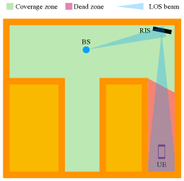
Figure 3: Indoor office scenario for BS-side RIS implementation [28].

V-A Simulation Setup

In this subsection, we describe two wireless communication scenarios to evaluate the performance of the proposed plug-in RIS in enhancing coverage. These scenarios have also presented in [28] as practical options for RIS implementation.

1. Indoor Office (BS-side RIS): The first scenario involves an indoor environment with two parallel hallways, as illustrated in Fig. 3. In practical situations, the BS is optimally installed to cover maximum areas, but due to mmWave vulnerability to blockage, certain spots and zones become challenging to cover, for instance, one of the parallel hallways in this scenario. Instead of deploying additional costly and inefficient BS, the RIS can be implemented to extend coverage to these dead zones. Here, the distance between the BS (RIS) and the RIS (UE) is $2.5\ m$ ($10\ m$).

2. Street Canyon (UE-side RIS): For the second scenario, we consider a street canyon environment, shown in Fig. 4, where the BS is installed on the rooftop of one building on one side of the street. UEs positioned along the same side of the street experience signal deficiency owing to their placement within the dead zone. While an alternative could involve deploying another BS on top of a building on the opposite side of the street, adopting RIS proves to be a more cost/energy-effective way to cover the dead zone. In this scenario, we assume that the distance between the BS (RIS) and the RIS (UE) is $20\ m$ ($10\ m$).

Figure 4: Street canyon scenario for UE-side RIS implementation.

This paper considers a limited and well-known dead zone [28], as depicted in Figs. 3 and 4, which leads to an assumption that the elevation AoD of the sub-RISs is constrained within a limited range. Consequently, we consider that the azimuth and elevation AoDs of the sub-RISs are $\varphi_{t,ris}\in\mathcal{U}[-\pi,\pi]$ and $\vartheta_{t,ris}\in\mathcal{U}[-\pi/16,\pi/16]$, respectively. With such assumptions and by adopting a sub-RIS of size $10\times 10$, the sub-RIS can cover a circular area with a diameter of $4\ m$ which is located $10$ m away from the sub-RIS. Furthermore, given the fixed position of BS and sub-RISs, we can align the sub-RISs optimally with the BS [20] to meet the desired minimum sub-RISs separation requirements. Based on our discussion in Section III and as given in Fig. 2 (a), we assume that $\varphi_{t},\varphi_{r,ris}\in\mathcal{U}[-\pi,\pi]$ and $\vartheta_{t},\vartheta_{r,ris}\in\mathcal{U}[-\pi/3,\pi/3]$, considering the BS is equipped with a $10\times 10$ antenna array. In other words, we assume that if the incident angle $\theta_{0}$ is confined to an interval of $[-\pi/3,\pi/3]$, the EFD remains constant. We can consider the maximum amount of EFD in this interval to calculate $\Delta$.

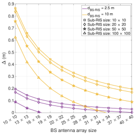
Figure 5: The variations of sub-RIS inter-spacing ($\Delta$) with respect to different BS antenna array sizes for different distances and sub-RIS sizes.

Fig. 5 depicts sub-RIS inter-spacing versus different system parameters. As shown in Fig. 5, with increasing BS antenna array size, the minimum spacing among sub-RISs $\Delta$ decreases due to narrower beams emitted through BS. On the other hand, with increasing the distance between BS and RIS, the EFD increases, which means that the sub-RISs inter-space should be increased to avoid power leakage to the non-targeted sub-RISs. Nevertheless, since the RIS is a passive device, we can increase the number of reflecting elements in each sub-RIS to decrease $\Delta$. This is specifically feasible in the proposed plug-in RIS since increasing the number of elements does not entail more complexity in the system. It is worth emphasizing that since the sub-RISs in the plug-in RIS exploit fixed beams, only traditional end-to-end channel estimation is enough, and cascaded channel decoupling is not required in the practical plug-in RIS system, resulting in significant complexity reduction in comparison with semi-passive and fully passive RIS structures, which allows us to easily increase the number of reflectors in the plug-in RIS structure. Fig. 5 shows that with increasing the sub-RIS size, the sub-RISs inter-space decreases. Note that in this paper, we consider BS antenna array and sub-RISs of size $10\times 10$ to prevent high computational burden in the computer simulations, since in the computer simulations, we need to construct the cascaded channels separately for the sake of analysis.

As depicted in Fig. 6, various segments within the receive dead zone are represented in polar coordinates for both two and four divisions. The fixed beam orientation for each segment and several potential UE positions within the dead zone are also illustrated in Fig. 6. It is worth mentioning that the information given in Fig. 6 is used for plug-in RIS configuration and dead zone segmentation in this paper. Specifically, for two and four spatial segments, $(\phi_{b,i},\theta_{b,i})\in\{(\pi/2,\pi/32),(-\pi/2,\pi/32)\}$ and $(\phi_{b,i},\theta_{b,i})\in\{(\pi/4,\pi/32),(3\pi/4,\pi/32),(-\pi/4,\pi/32),(-3\pi/4,\pi/32)\}$, respectively. As the number of segments increases, the average distance between the UE positions and the corresponding fixed beam orientations decreases; consequently, the UEs can receive signals via more favorable beams, which enhances overall system performance. It is important to mention that although Fig. 6 shows dead zone division only along the azimuth angle, such division can also be applied along the elevation angle. However, for clarity and simplicity, we have opted not to illustrate more complex divisions in the figures.

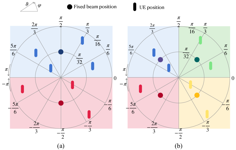
Figure 6: Dead zone divisions, fixed beams, and possible UE positions for (a) two segments and (b) four segments.

TABLE II: Simulation parameters.

Parameter Description Value $f_{c}$ Carrier frequency $28$ GHz $B$ Bandwidth $100$ MHz $N_{t}$ BS antenna array size $10\times 10$ $N_{r}$ UE antenna array size $1$ $\delta_{x}=\delta_{y}$ Antenna element separation $\lambda/2$ Noise PSD Noise power spectral density $-174$ dBm $g_{e}$ Antenna element gain $0$ dBi $\varphi_{t}$ ($\varphi_{r,ris}$) Azimuth Tx AoD (RIS AoA) $\mathcal{U}[-\pi,\pi]$ $\varphi_{t,ris}$ Azimuth RIS AoD $\mathcal{U}[-\pi,\pi]$ $\vartheta_{t}$ ($\vartheta_{r,ris}$) Elevation Tx AoD (RIS AoA) $\mathcal{U}[-\pi/3,\pi/3]$ $\vartheta_{t,ris}$ Elevation RIS AoD $\mathcal{U}[-\pi/16,\pi/16]$ $(\phi_{b,k},\theta_{b,k})$ Azimuth and elevation AoD for a two sub-RIS system $\{(\frac{\pi}{2},\frac{\pi}{32})$,$(-\frac{\pi}{2},\frac{\pi}{32})\}$ $(\phi_{b,k},\theta_{b,k})$ Azimuth and elevation AoD for a four sub-RIS system $\{(\frac{\pi}{4},\frac{\pi}{32})$,$(\frac{3\pi}{4},\frac{\pi}{32})$, $(-\frac{\pi}{4},\frac{\pi}{32})$,$(-\frac{3\pi}{4},\frac{\pi}{32})\}$ $P_{\text{PA}}$ Power amplifier power consumption $20$ mW [30] $N_{\text{rf}}$ Number of RF chain $1$ $M_{\text{active}}$ Number of RIS active elements $0.08\times M$ [9] $P_{\text{PS}}$ Phase shifter power consumption $30$ mW [30] $P_{\text{RF-chain}}$ RF chain power consumption $40$ mW [31, 30] $P_{\text{BB}}$ Baseband processor power consumption $200$ mW [31, 30] $P_{\text{LNA}}$ Low noise amplifier power consumption $20$ mW [31, 30] $P_{\text{PA\_RIS}}$ RIS element power consumption $10$ mW [10] $FOM_{W}$ Walden’s figure-of-merit $46.1$ fJ/conversion-step [10] Indoors $(a,b)$ Path loss parameters $(32.4,1.73)$ [32] $d_{BR}$ Distance between BS and RIS $2.5\ m$ $d_{RU}$ Distance between RIS and UE $10\ m$ Outdoors $(a,b)$ Path loss parameters $(32.4,2.1)$ [32] $d_{BR}$ Distance between BS and RIS $20\ m$ $d_{RU}$ Distance between RIS and UE $10\ m$

The carrier frequency is designated as $28$ GHz, and the path loss model is employed as follows [32]:

$$PL(d)=a+10b\log_{10}{(d)}+20\log_{10}{(f_{c})},$$ (19)

where the values of $a$ and $b$ are given in Table II. The analysis assumes a noise power spectral density (PSD) of $-174$ dBm/Hz, with a bandwidth ($B$) of $100$ MHz [20]. This results in a noise power calculation of $\sigma^{2}=-94$ dBm [20]. The antenna gain of each element is considered to be $g_{e}=0$ dBi, signifying the utilization of omnidirectional antennas for every element. The assumed values for system parameters are summarized in Table II.

It is noteworthy that in this paper the system performance analysis is carried out using two and four sub-RIS configurations. During each transmission period, only one sub-RIS is used while the rest remain idle. On the other hand, the semi-passive RIS utilizes all implemented elements for maximum performance. In other words, the plug-in RIS uses only a portion of deployed elements, potentially sacrificing passive beamforming gain compared to the semi-passive RIS. However, the semi-passive RIS employs baseband components to estimate the cascaded channels and adjust its phase shifts autonomously, while the proposed plug-in RIS remains fully passive. Therefore, the plug-in RIS offers a favorable trade-off between system performance and EE/cost/complexity. Likewise, for the blind RIS, all implemented elements are engaged in each transmission cycle.

V-B Examining ABER Performance and Theoretical Validation

This subsection displays simulation results for the ABER performance of the proposed plug-in RIS. We further verify these results via the analytical upper bound derived in Lemma 3. Here, we utilize a $10\times 10$ RIS for the semi-passive RIS structure to match the passive beamforming gain with the proposed plug-in RIS in each transmission period (since in each transmission period, only one sub-RIS of size $10\times 10$ is used). In contrast, for the blind RIS design, we consider RIS sizes of $20\times 10$ and $20\times 20$ to highlight the superiority of the plug-in RIS over blind RIS.

As depicted in Fig. 7, our simulations closely align with the upper bound, confirming the accuracy of the conducted simulations for both indoor office and street canyon scenarios. Notably, we utilized a binary phase shift keying (BPSK) signaling scheme for this simulation. Fig. 7 illustrates a substantial performance improvement exhibited by the proposed plug-in RIS when compared with the blind RIS design, even though the blind RIS configuration considered here offers a larger beamforming gain due to its bigger size. Additionally, results in Fig. 7 reveal that adopting a plug-in RIS with two sub-RISs results in roughly $9$ dB higher ABER compared to the semi-passive RIS. On the other hand, employing four sub-RISs leads to performance enhancement, causing only a $2$ dB ABER degradation compared to the semi-passive RIS in both scenarios. It is important to recall that each sub-RIS corresponds to a segment within the dead zone, as shown in Fig. 6. Therefore, increasing the number of sub-RISs is equivalent to increasing the number of segments. Consequently, when we increase the sub-RISs from two to four, the ABER performance improves by about $7$ dB because the UE has more chance to receive a stronger signal. These outcomes underline the efficacy of the proposed plug-in RIS structure, which proves to be more cost-effective than the semi-passive alternative with a few degradations in ABER.

Figure 7: ABER performance analysis for (a) the BS-side RIS-aided system in the indoor office environment, (b) the UE-side RIS-aided system in the street canyon environment.

V-C Analysis of Achievable Rate Performance

In this subsection, we examine the achievable rate performance of the proposed plug-in RIS and compare it with benchmarks. For this subsection, alongside the RIS sizes explored in the previous subsection, we consider an RIS of size of $10\times 10$ for the blind RIS scheme. The achievable rate can be calculated as

$$R=\mathbb{E}[\log_{2}(1+\textrm{SNR})],$$ (20)

where SNR stands for signal-to-noise ratio and can be calculated as follows:

$$\textrm{SNR}=\frac{|\sqrt{P}G_{t}G_{r}\mathbf{f}_{r}^{H}\mathbf{H}_{\text{eff},k}\mathbf{f}_{t}|^{2}}{\sigma^{2}}.$$ (21)

Fig. 8 depicts the plug-in RIS performance in terms of achievable rate compared to the two considered benchmark schemes. Similar to the ABER performance, the plug-in RIS exhibits satisfactory achievable rate performance compared to the two benchmark schemes under consideration. Compared with the blind RIS configuration, our novel plug-in RIS configuration significantly improves the achievable rate performance. Likewise, similar to the ABER performance outcomes, even larger-scale blind RIS configurations, which provide more significant beamforming gains, fail to reach the achievable rate performance offered by the plug-in RIS configuration. In comparison to the semi-passive RIS, the proposed plug-in RIS shows a performance degradation of $5$ dB with $2$ sub-RISs. This degradation decreases to $2$ dB when using $4$ sub-RISs, demonstrating the impact of higher SNR at the UE due to increased segments in the dead zone.

Computer simulation results in this subsection emphasize the effectiveness of our plug-in RIS compared to the benchmarks. While the plug-in RIS may not outperform the semi-passive RIS, its cost-effective passive design merits consideration.

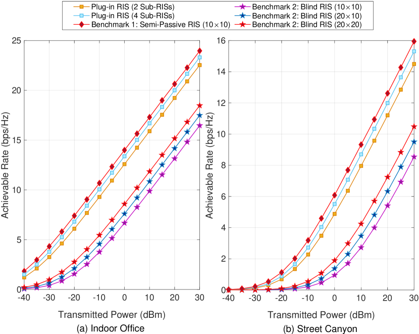
Figure 8: Achievable rate performance for (a) the BS-side RIS-aided system in the indoor office environment, (b) the UE-side RIS-aided system in the street canyon environment.

V-D Energy Efficiency Analysis

In this subsection, we focus on the strength point of the plug-in RIS design, which is its EE. We also highlight the trade-offs between EE and ABER/achievable rate. The EE is computed as follows:

$$\eta_{EE}=\frac{R\times B}{P_{c}}\ \text{bits/Joule},$$ (22)

where $P_{c}$ signifies the power consumption within the system and can be determined as follows [10]:

$$P_{c}=P_{\text{Tx}}+P_{\text{Rx}}+P_{\text{RIS}},$$ (23)

where $P_{i}$ ($i\in\{\text{Tx, Rx, RIS}\}$) denotes the power consumption of the respective terminal and can be calculated as follows [30, 31]:

$$\begin{split}P_{\text{Tx}}=P+N_{t}&P_{\text{PA}}+N_{\text{rf}}(N_{t}P_{\text{PS}}+P_{\text{RF-chain}}+2P_{\text{DAC}})+P_{\text{BB}},\end{split}$$ (24)

$$\begin{split}P_{\text{Rx}}=N_{r}P_{\text{LNA}}&+N_{\text{rf}}(N_{r}P_{\text{PS}}+P_{\text{RF-chain}}+2P_{\text{ADC}})+P_{\text{BB}},\end{split}$$ (25)

$$P_{\text{RIS(Passive)}}=MP_{\text{PA\_RIS}},$$ (26)

$$\begin{split}P_{\text{RIS(Semi\_Passive})}=&MP_{\text{PA\_RIS}}+M_{\text{active}}(P_{\text{LNA}}\\ &+P_{\text{RF-chain}}+2P_{\text{ADC(RIS)}})+P_{\text{BB}},\end{split}$$ (27)

where $M$ represents for number of RIS/sub-RIS elements engaged in the communication and $P_{\text{ADC}}$ ($P_{\text{DAC}}$) is the consumption power of analog-to-digital (ADC) (digital-to-analog (DAC)) converter at the receive (transmit) terminal and can be computed as follows [10, 31]:

$$P_{\text{ADC}}=P_{\text{DAC}}=FOM_{W}\times f_{s}\times 2^{b},$$ (28)

where $FOM_{W}$ corresponds to Walden’s figure-of-merit for assessing ADC power efficiency, the variable $f_{s}$ stands for the Nyquist sampling frequency, while $b$ represents the ADC resolution bits. Our assumption employs $FOM_{W}=46.1$ fJ/conversion-step for a $100$ MHz bandwidth [10]. We utilize ADCs with $1$ bit and $4$ bits resolution for the semi-passive RIS [9] and transceivers [31], respectively. We also consider $8\%$ of elements in the semi-passive RIS being connected to baseband components as suggested in [9]. All other parameters align with those defined in Table II.

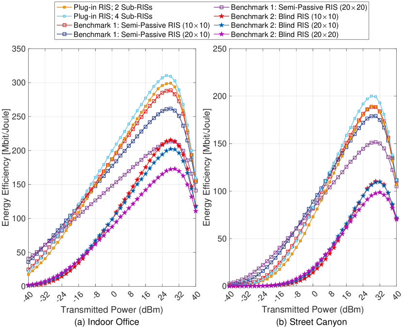
Figure 9: Energy efficiency comparison for (a) the BS-side RIS-aided system in the indoor office environment, (b) the UE-side RIS-aided system in the street canyon environment.

As illustrated in Fig. 9, the plug-in RIS performs better than both benchmarks in indoor and outdoor scenarios. The performance of the plug-in RIS improves as the number of sub-RISs increases, benefiting from higher SNR and the power-efficient nature of passive elements. Essentially, increasing the number of sub-RISs allows for increasing the number of segments within the dead zone. Consequently, each segment becomes smaller, leading to improved received SNR and better $\eta_{EE}$. On the contrary, increasing the number of elements in the semi-passive RIS negatively affects EE and leads to performance deterioration. It is important to note that although enlarging the RIS size in the semi-passive RIS configuration increases received SNR due to enhanced beamforming gain, it also involves more baseband components in the RIS structure, resulting in higher power consumption. In this case, power consumption primarily impacts EE performance and leads to decreased EE.

In the case of the blind RIS, different behaviors are observed in two scenarios. In the indoor scenario, increasing the number of elements does not improve EE. Fig. 9 (a) shows that increasing the dimension of the blind RIS reduces EE due to the dominant effect of power consumption by passive elements. In contrast, in the outdoor scenario, increasing the number of elements from $10\times 10$ to $20\times 10$ leads to positive effects on beamforming gain, but power consumption also increases proportionally, resulting in no change in EE. However, a larger RIS size in the outdoor scenario, i.e., $20\times 20$, repeats the indoor scenario’s behavior, with power consumption becoming dominant and causing EE degradation. It is worth mentioning that a notable EE performance gap exists between blind RIS and the proposed plug-in RIS, primarily due to the enhanced SNR provided by the plug-in RIS without a proportional increase in power consumption.

V-E Detector Complexity

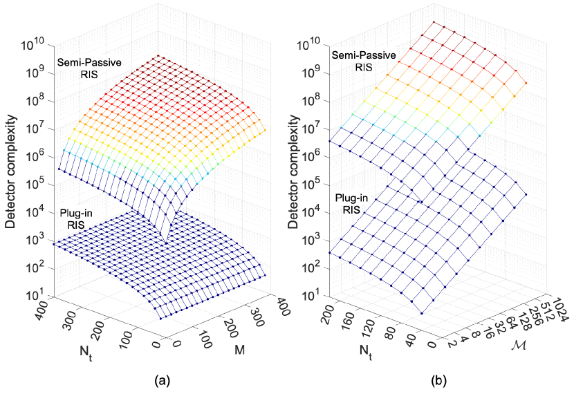
Figure 10: Detector complexity comparison as a function of (a) number of transmit antennas, $N_{t}$, and number of RIS elements, $M$, (b) number of transmit antennas, $N_{t}$, and constellation order, $\mathcal{M}$.

The detector complexity for different numbers of transmit antennas, RIS elements, and constellation orders is depicted in Fig. 10. As shown in Fig. 10 (a), it is evident that the plug-in RIS’s detector exhibits significantly lower computational complexity compared to the semi-passive RIS’s detector. It is worth noting that the increase in the number of RIS elements ($M$) has a more significant impact on the complexity of the semi-passive RIS detector compared to the increase in the number of antennas ($N_{t}$); this is attributed to the quadratic relationship between $M$ and the detector complexity in the semi-passive detector expression, while the plug-in RIS design remains unaffected by the increase in $M$. Note that in Fig. 10 (a), we have considered $\mathcal{M}=2$. Fig. 10 (b) further illustrates how variations in $N_{t}$ and $\mathcal{M}$ affect detector complexity while maintaining a constant number of RIS elements ($M=100$), emphasizing the superiority of the proposed plug-in RIS over semi-passive RIS design.

VI Conclusion

This paper has introduced a practical RIS structure, the plug-in RIS, for mmWave communication systems to enhance coverage to the dead zones. The plug-in RIS operates passively, cleverly integrating the control mechanism within the transmitted beam to the RIS, eliminating the need for conventional reliable control links. It also relaxes the channel estimation process by eliminating complex cascaded channel decoupling, a common challenge in RIS-assisted systems. In this approach, dead zones are divided into segments, each served by a dedicated sub-RIS with a fixed beam. Computer simulation results have shown that deploying four sub-RISs causes only slight degradation in ABER and achievable rates, making fully passive operation feasible. We have also compared the EE of the plug-in RIS with benchmarks. While the semi-passive RIS slightly outperforms the plug-in RIS in terms of ABER and achievable rate, its EE performance is worse than the proposed plug-in RIS due to active baseband components. Besides, the plug-in RIS detector exhibits superior complexity performance compared to the semi-passive RIS thanks to the conventional channel estimation mechanism.

In summary, our plug-in RIS proves to be a compelling solution, performing closely to the semi-passive RIS regarding ABER and achievable rate performances, surpassing the benchmarks in terms of EE performance and detector complexity, and addressing challenges in mmWave systems. Unlike traditional RIS designs, plug-in RIS allows simultaneously serving multiple UEs within the same spatial segment. Nonetheless, such a scenario requires careful interference mitigation design, which remains a topic for future research endeavors.

Appendix A Proof of Corollary 1

By substituting $\theta_{0}=0$ into (13), we can simplify it as:

$$\textrm{EFD}=2d\times\tan(\frac{\textrm{HPBW}}{2}).$$ (29)

On the other hand, the tangent function can be expanded using the MacLaurin series as follows:

$$\tan(x)=x+\frac{x^{3}}{3}+\frac{2x^{5}}{15}+\dots;\ \ \textrm{if}\ \ |x|<\frac{\pi}{2},$$ (30)

whereas when $x$ is of a small magnitude, it can be approximated as $\tan(x)\approx x$. Note that $\frac{\textrm{HPBW}}{2}$ becomes relatively small when implementing a massive MIMO array at the BS. Consequently, the approximation formula remains applicable here, and we can further simplify (29) to (14).

Appendix B Proof of Lemma 3

By exploiting [20, equation (24)] and after some mathematical manipulations, (16) can be updated as

$$\begin{split}\mathcal{P}(s^{*}\rightarrow&\hat{s}|\alpha_{k},\beta_{k})=\mathcal{P}(|\sqrt{P}G_{t}G_{r}\mathbf{f}_{r}^{H}\mathbf{H}_{\text{eff},k}\mathbf{f}_{t}(s^{*}-\hat{s})|^{2}\\ &+2\mathcal{R}\{\sqrt{P}G_{t}G_{r}\mathbf{n}^{H}\mathbf{f}_{r}\mathbf{f}_{r}^{H}\mathbf{H}_{\text{eff},k}\mathbf{f}_{t}(s^{*}-\hat{s})<0\}).\end{split}$$ (31)

As the elements of $\mathbf{n}^{H}$ follows a complex normal distribution with variance $\sigma^{2}$, its real component also conforms to a normal distribution with variance $\frac{\sigma^{2}}{2}$, represented as $\mathcal{R}\{\mathbf{n}^{H}\}\sim\mathcal{N}(\mathbf{0}_{N_{r}},\frac{\sigma^{2}}{2}\mathbf{I}_{N_{r}})$. Consequently, we can readily express:

$$\begin{split}\mathcal{R}\{A\mathbf{n}^{H}\}+\mu\mathbf{1}_{N_{r}}^{H}\sim\mathcal{N}(\mu\mathbf{1}_{N_{r}},\frac{A^{2}\sigma^{2}}{2}\mathbf{I}_{N_{r}}),\end{split}$$ (32)

where $A=2\sqrt{P}G_{t}G_{r}||\mathbf{f}_{r}\mathbf{f}_{r}^{H}\mathbf{H}_{\text{eff},k}\mathbf{f}_{t}(s^{*}-\hat{s})||$ and $\mu=|\sqrt{P}G_{t}G_{r}\mathbf{f}_{r}^{H}\mathbf{H}_{\text{eff},k}\mathbf{f}_{t}(s^{*}-\hat{s})|^{2}$; accordingly, (31) can be calculated as

$$\begin{split}\mathcal{P}(s^{*}\rightarrow&\hat{s}|\alpha_{k},\beta_{k})=Q(\sqrt{2}\frac{\mu}{A\sigma})\\ &=Q(\frac{\sqrt{P}G_{t}G_{r}|\mathbf{f}_{r}^{H}\mathbf{H}_{\text{eff},k}\mathbf{f}_{t}(s^{*}-\hat{s})|^{2}}{\sqrt{2}\sigma||\mathbf{f}_{r}\mathbf{f}_{r}^{H}\mathbf{H}_{\text{eff},k}\mathbf{f}_{t}(s^{*}-\hat{s})||}).\end{split}$$ (33)

References

- [1] E. Basar, M. Di Renzo, J. De Rosny, M. Debbah, M.-S. Alouini, and R. Zhang, “Wireless communications through reconfigurable intelligent surfaces,” IEEE Access, vol. 7, pp. 116753–116773, Aug. 2019.
- [2] D. Mishra and H. Johansson, “Channel estimation and low-complexity beamforming design for passive intelligent surface assisted MISO wireless energy transfer,” in 2019 IEEE Int. Conf. Acoust. Speech Signal Process. (ICASSP), Brighton, UK, pp. 4659–4663, May 2019.
- [3] P. Wang, J. Fang, H. Duan, and H. Li, “Compressed channel estimation for intelligent reflecting surface-assisted millimeter wave systems,” IEEE Signal Process. Lett., vol. 27, pp. 905–909, May. 2020.
- [4] J. Chen, Y.-C. Liang, H. V. Cheng, and W. Yu, “Channel estimation for reconfigurable intelligent surface aided multi-user mmWave MIMO systems,” IEEE Trans. Wirel. Commun., pp. 1–1, Feb. 2023.
- [5] T. Lin, X. Yu, Y. Zhu, and R. Schober, “Channel estimation for intelligent reflecting surface-assisted millimeter wave MIMO systems,” in 2020 IEEE Glob. Commun. Conf. (GLOBECOM), Taipei, Taiwan, pp. 1–6, Dec. 2020.
- [6] Z.-Q. He and X. Yuan, “Cascaded channel estimation for large intelligent metasurface assisted massive MIMO,” IEEE Wireless Commun. Lett., vol. 9, pp. 210–214, Oct. 2020.
- [7] C. Hu, L. Dai, S. Han, and X. Wang, “Two-timescale channel estimation for reconfigurable intelligent surface aided wireless communications,” IEEE Trans. Commun., vol. 69, pp. 7736–7747, Apr. 2021.
- [8] Z. Wan, Z. Gao, and M.-S. Alouini, “Broadband channel estimation for intelligent reflecting surface aided mmWave massive MIMO systems,” in 2020 IEEE Int. Conf. Commun. (ICC), Dublin, Ireland, pp. 1–6, Jun. 2020.
- [9] J. Hu, H. Yin, and E. Björnson, “MmWave MIMO communication with semi-passive RIS: A low-complexity channel estimation scheme,” in 2021 IEEE Glob. Commun. Conf. (GLOBECOM), Madrid, Spain, pp. 01–06, Dec. 2021.
- [10] A. Taha, M. Alrabeiah, and A. Alkhateeb, “Enabling large intelligent surfaces with compressive sensing and deep learning,” IEEE Access, vol. 9, pp. 44304–44321, Mar. 2021.
- [11] Y. Jin, J. Zhang, X. Zhang, H. Xiao, B. Ai, and D. W. K. Ng, “Channel estimation for semi-passive reconfigurable intelligent surfaces with enhanced deep residual networks,” IEEE Trans. Veh. Technol., vol. 70, pp. 11083–11088, Sep. 2021.
- [12] F. Zheng, H. Liu, and L. Chi, “A semi-passive RIS channel estimation method based on super-resolution network,” in 2022 IEEE 8th Int. Conf. Comput. Commun. (ICCC), Chengdu, China, pp. 17–21, Mar. 2022.
- [13] Z. Zhang, L. Dai, X. Chen, C. Liu, F. Yang, R. Schober, and H. V. Poor, “Active RIS vs. passive RIS: Which will prevail in 6G?,” IEEE Trans. Commun., vol. 71, no. 3, pp. 1707–1725, 2023.
- [14] Reconfigurable Intelligent Surfaces (RIS); Communication Models, Channel Models, Channel Estimation and Evaluation Methodology. ETSI GR RIS 003 V1.1.1, May. 2023.
- [15] M. Raeisi, A. Koc, I. Yildirim, E. Basar, and T. Le-Ngoc, “Antenna array structures for enhanced cluster index modulation,” in 2023 Joint Eur. Conf. Netw. Commun. & 6G Summit (EuCNC/6G Summit), Gothenburg, Sweden, pp. 102–107, Jun. 2023.
- [16] P. Wang, J. Fang, L. Dai, and H. Li, “Joint transceiver and large intelligent surface design for massive MIMO mmWave systems,” IEEE Trans. Wireless. Commun., vol. 20, pp. 1052–1064, Oct. 2020.
- [17] P. Wang, J. Fang, X. Yuan, Z. Chen, and H. Li, “Intelligent reflecting surface-assisted millimeter wave communications: Joint active and passive precoding design,” IEEE Trans. Veh. Technol., vol. 69, pp. 14960–14973, Oct. 2020.
- [18] K. Ying, Z. Gao, S. Lyu, Y. Wu, H. Wang, and M.-S. Alouini, “GMD-based hybrid beamforming for large reconfigurable intelligent surface assisted millimeter-wave massive MIMO,” IEEE Access, vol. 8, pp. 19530–19539, Jan. 2020.
- [19] M. Raeisi, A. Koc, E. Basar, and T. Le-Ngoc, “Cluster index modulation for mmWave communication systems,” Front. Comms. Net., Feb. 2022.
- [20] M. Raeisi, A. Koc, I. Yildirim, E. Basar, and T. Le-Ngoc, “Cluster index modulation for reconfigurable intelligent surface-assisted mmWave massive MIMO,” IEEE Trans. Wireless Commun., pp. 1–1, 2023.
- [21] P. Hannan, “The element-gain paradox for a phased-array antenna,” IEEE Trans. Antennas Propag., vol. 12, pp. 423–433, Jul. 1964.
- [22] H. Sarieddeen, M.-S. Alouini, and T. Y. Al-Naffouri, “Terahertz-band ultra-massive spatial modulation MIMO,” IEEE J. Sel. Areas Commun., vol. 37, pp. 2040–2052, Sep. 2019.
- [23] S. Gopi, S. Kalyani, and L. Hanzo, “Intelligent reflecting surface assisted beam index-modulation for millimeter wave communication,” IEEE Trans. Wireless Commun., vol. 20, pp. 983–996, Oct. 2020.
- [24] C. A. Balanis, Antenna Theory: Analysis and Design. John wiley & sons, 2015.
- [25] H. L. Van Trees, Optimum Array Processing: Part IV of Detection, Estimation, and Modulation Theory. John Wiley & Sons, 2002.
- [26] K. Ntontin, A.-A. A. Boulogeorgos, D. G. Selimis, F. I. Lazarakis, A. Alexiou, and S. Chatzinotas, “Reconfigurable intelligent surface optimal placement in millimeter-wave networks,” IEEE open j. Commun. Soc., vol. 2, pp. 704–718, Mar. 2021.
- [27] E. Basar, “Transmission through large intelligent surfaces: A new frontier in wireless communications,” in 2019 Eur. Conf. on Netw. and Commun. (EuCNC), Valencia, Spain, pp. 112–117, Jun. 2019.
- [28] Reconfigurable Intelligent Surfaces (RIS); Use Cases, Deployment Scenarios and Requirements. ETSI GR RIS 001 V1.1.1, Apr. 2023.
- [29] R. Peng and Y. Tian, “Robust wide-beam analog beamforming with inaccurate channel angular information,” IEEE Commun. Lett., vol. 22, pp. 638–641, Mar. 2018.
- [30] R. Méndez-Rial, C. Rusu, N. González-Prelcic, A. Alkhateeb, and R. W. Heath, “Hybrid MIMO architectures for millimeter wave communications: Phase shifters or switches?,” IEEE Access, vol. 4, pp. 247–267, 2016.
- [31] J. Mo, A. Alkhateeb, S. Abu-Surra, and R. W. Heath, “Hybrid architectures with few-bit ADC receivers: Achievable rates and energy-rate tradeoffs,” IEEE Trans. Wireless Commun., vol. 16, no. 4, pp. 2274–2287, 2017.
- [32] 5G: Study on Channel Model for Frequencies from 0.5 to 100 GHz. document 3GPP TR 38.901, Ver. 17.0.0, Apr. 2022.