Comprehensive Evaluation and Insights into the Use of Deep Neural Networks to Detect and Quantify Lymphoma Lesions in PET/CT Images

Abstract

This study performs comprehensive evaluation of four neural network architectures (UNet, SegResNet, DynUNet, and SwinUNETR) for lymphoma lesion segmentation from PET/CT images. These networks were trained, validated and tested on a diverse, multi-institutional dataset of 611 cases. Internal testing (88 cases; total metabolic tumor volume (TMTV) range [0.52, 2300] ml) showed SegResNet as the top performer with a median Dice similarity coefficient (DSC) of 0.76 and median false positive volume (FPV) of 4.55 ml; all networks had a median false negative volume (FNV) of 0 ml. On the unseen external test set (145 cases with TMTV range: [0.10, 2480] ml), SegResNet achieved the best median DSC of 0.68 and FPV of 21.46 ml, while UNet had the best FNV of 0.41 ml. We assessed reproducibility of six lesion measures, calculated their prediction errors, and examined DSC performance in relation to these lesion measures, offering insights into segmentation accuracy and clinical relevance. Additionally, we introduced three lesion detection criteria, addressing the clinical need for identifying lesions, counting them, and segmenting based on metabolic characteristics. We also performed expert intra-observer variability analysis revealing the challenges in segmenting “easy” vs. “hard” cases, to assist in the development of more resilient segmentation algorithms. Finally, we performed inter-observer agreement assessment underscoring the importance of a standardized ground truth segmentation protocol involving multiple expert annotators. Code is available at: https://github.com/microsoft/lymphoma-segmentation-dnn.

Positron emission tomography, computed tomography, deep learning, segmentation, detection, lesion measures, intra-observer variability, inter-observer variability.

1 Introduction

fluorodeoxyglucose (¹⁸F-FDG) PET/CT imaging is the standard of care for lymphoma patients, providing accurate diagnoses, staging, and therapy response evaluation. However, traditional qualitative assessments, like Deauville scores [1], can introduce variability due to observer’s subjectivity in image interpretation. Using quantitative PET analysis that incorporates lesion measures such as mean lesion standardized uptake value ($\text{SUV}_{\text{mean}}$), total metabolic tumor volume (TMTV), and total lesion glycolysis (TLG) offers a promising path to more reliable prognostic decisions, enhancing our ability to predict patient outcomes in lymphoma with greater precision and confidence [2].

Quantitative assessment in PET/CT imaging often relies on manual lesion segmentation, which is time-consuming and prone to intra- and inter-observer variabilities. Traditional thresholding-based automated techniques can miss low-uptake disease and produce false positives in regions of physiological high uptake of radiotracers. Therefore, deep learning offers promise for automating lesion segmentation, reducing variability, increasing patient throughput, and potentially aiding in the detection of challenging lesions [3].

Although promising, deep learning methods face challenges of their own. Convolutional neural networks (CNNs) require large, well-annotated datasets that can be difficult to obtain. Models trained on small datasets may not be generalizable. Moreover, lymphoma lesions vary significantly in size, shape, and metabolic activity, making training deep networks accurately challenging in the absence of well-defined priors. Deep learning aims to reduce observer variability, but inconsistent manual annotations used for training can lead to error perpetuation. Understanding these challenges is crucial towards harnessing the full potential of these methods in PET/CT quantitative analysis.

2 Related work

Numerous works have explored the application of deep learning methods for segmenting lymphoma in PET/CT images. Yuan et al. [4] developed a feature fusion technique to utilize the complementary information from multi-modality data. Hu et al. [5] proposed fusing a combination of 3D ResUNet trained on volumetric data and three 2D ResUNet trained on 2D slices from three orthogonal directions for enhancing segmentation performance. Li et al. [6] proposed DenseX-Net trained in an end-to-end fashion integrating supervised and unsupervised methods for lymphoma detection and segmentation. Liu et al. [7] introduced techniques such as patch-based negative sample augmentation and label guidance for training a 3D Residual-UNet for lymphoma segmentation. A major limitation of all these works was that they were developed on relatively smaller-sized datasets (less than 100 images). Moreover, most of these methods did not compare the performance of their proposed methods with other baselines or with the performance of physicians.

Constantino et al. [8] compared the performances of 7 semi-automated and 2 deep learning segmentation methods, while Weisman et al. [9] compared 11 automated segmentation techniques, although both these studies were performed on smaller datasets of sizes 65 and 90 respectively. Weisman et al. [10] compared the segmentation performances of automated 3D Deep Medic method with that of physician although even this study included just 90 lymphoma cases. Except for [10], none of these studies reported model generalization on out-of-distribution dataset (such as on data collected from different centers), limiting their robustness quantification and external validity. Jiang et al. [11] used a relatively larger dataset as compared to the above studies with 297 images to train a 3D UNet. They even performed out-of-distribution testing on 117 images collected from a different center. To the best of our knowledge, the largest lymphoma PET/CT dataset for deep learning-based lesion segmentation ever reported is the work by Blanc-Durand et al. [12] who used 639 images for model development and 94 for external testing; however, this study only used standard segmentation evaluation metrics and assessed their model’s ability for predicting accurate TMTV. Both the studies [11] and [12] are limited by the fact that their datasets exclusively consisted of patients diagnosed with diffuse large B-cell lymphoma (DLBCL), representing only a single subtype of lymphoma.

Most of the existing studies on deep learning-based lymphoma segmentation report their performances on generic segmentation metrics such as Dice similarity coefficient (DSC), intersection-over-union (IoU), sensitivity, etc. In the presence of large segmented lesions, very small missed lesions or small false positives do not contribute much to the DSC value. Hence, there is a need to report the volumes of false positives and false negatives. It will also be beneficial to evaluate the detection performances on a per-lesion basis (number of connected components detected vs missed), since automated detection of even a few voxels of all lesions can help physicians quickly locate the regions of interest, even if the DSC is low. Moreover, the difficulty of the segmentation/detection task is often not assessed via inter- or intra-observer agreement analysis.

The segmentation performance of networks in medical imaging often relies on various critical lesion features, such as $\text{SUV}_{\text{mean}}$, $\text{SUV}_{\text{max}}$, and TMTV [13], which are usually poorer for small and faint lesions. However, the existing studies usually do not report the distribution of these lesion features within privately-owned datasets, leading to a lack of transparency regarding dataset properties. This knowledge gap impedes the understanding of the relationship between segmentation model performance and dataset characteristics, ultimately limiting the scalability and translation of these approaches into clinical practice. Addressing this issue requires researchers to provide comprehensive dataset information, as well as to evaluate the dependence of network performance on these lesion features.

Our study aims to address these limitations. We trained and validated four deep neural networks on lymphoma PET/CT datasets from three cohorts, encompassing two distinct subtypes of lymphoma: DLBCL and primary mediastinal large B-cell lymphoma (PMBCL). (i) We performed both in (images coming from same cohorts as the training/validation set) and out-of-distribution or external (images from a fourth cohort not used for training/validation) testing to evaluate the robustness of our models. (ii) We reported the performance using DSC, volumes of false positives and negatives, and evaluated the performance dependence on six different types of lesion measures. (iii) We also evaluated the ability of our networks to reproduce these ground truth lesion measures and computed networks’ error in predicting them. (iv) We proposed three types of detection criteria for our use-case and evaluate model’s performance on these metrics. (v) Finally, we evaluated the intra- and inter-observer agreement to give a measure of the difficulty of lesion segmentation task on our datasets.

3 Materials and Methods

3.1 Dataset

3.1.1 Description

In this work, we used a large, diverse and multi-institutional whole-body PET/CT dataset with a total of 611 cases. These scans came from four retrospective cohorts: (i) DLBCL-BCCV: 107 scans from 79 patients with DLBCL from BC Cancer, Vancouver (BCCV), Canada; (ii) PMBCL-BCCV: 139 scans from 69 patients with PMBCL from BC Cancer; (iii) DLBCL-SMHS: 220 scans from 219 patients with DLBCL from St. Mary’s Hospital, Seoul (SMHS), South Korea; (iv) AutoPET lymphoma: 145 scans from 144 patients with lymphoma from the University Hospital Tübingen, Germany [14]. Additional description on the number of scans, patient age and sex, and manufacturers of PET/CT scanner for each cohort is given in Table 1. The cohorts (i)-(iii) are collectively referred to as the internal cohort. For cohorts (i) and (ii), ethics approval was granted by the UBC BC Cancer Research Ethics Board (REB) (REB Numbers: H19-01866 and H19-01611 respectively) on 30 Oct 2019 and 1 Aug 2019 respectively. For cohort (iii), the approval was granted by St. Mary’s Hospital, Seoul (REB Number: KC11EISI0293) on 2 May 2011. Due to the retrospective nature of our data, patient consent was waived for these three cohorts. The cohort (iv) was obtained from the publicly available AutoPET challenge dataset [14] and is referred to as the external cohort.

Cohort	Institution	Number of patients/scans; Age in years (median & range); Sex	Number of scans on PET/CT scanners from different manufacturers
DLBCL-BCCV (internal)	BC Cancer, Vancouver, Canada	79/107; 69 [19, 89]; M/F: 37/42	GE Medical Systems: 102; Siemens: 5
PMBCL-BCCV (internal)	BC Cancer, Vancouver, Canada	69/139 33 [19, 79]; M/F: 30/39	GE Medical Systems: 119; Siemens: 20
DLBCL-SMHS (internal)	St. Mary’s Hospital, Seoul, South Korea	219/220; 61 [14, 87]; M/F: 117/102	Siemens: 220
AutoPET lymphoma (external)	University Hospital Tübingen, Germany	144/145; 47 [11, 85]; M/F: 76/88	Siemens: 145

Table 1: Patient and scan characteristics across four different lymphoma cohorts.

3.1.2 Ground truth annotation

The DLBCL-BCCV, PMBCL-BCCV, and DLBCL-SMHS cohorts were separately segmented by three nuclear medicine physicians (referred to as Physician 1, Physician 4, and Physician 5, respectively) from BC Cancer, Vancouver, BC Children’s Hospital, Vancouver, and St. Mary’s Hospital, Seoul, respectively. Additionally, two other nuclear medicine physicians (Physicians 2 and 3) from BC Cancer segmented 9 cases from DLBCL-BCCV cohort which were used for assessing the inter-observer variability (Section 4.4). Physician 4 additionally re-segmented 60 cases from PMBCL-BCCV cohort which were used for assessing the intra-observer variability (Section 4.3). All these expert segmentations were performed using the semi-automatic gradient-based segmentation tool called PETEdge+ from the MIM workstation (MIM software, Ohio, USA).

The AutoPET lymphoma PET/CT data along with their ground truth segmentations were acquired from The Cancer Imaging Archive. These annotations were performed manually by two radiologists from the University Hospital Tübingen, Germany, and the University Hospital of the LMU, Germany.

3.2 Networks, tools and code

Four networks were trained in this work, namely, UNet [15], SegResNet [16], DynUNet [17] and SwinUNETR [18]. The former three are 3D CNN-based networks, while SwinUNETR is a transformer-based network. The implementations for these networks were adapted from the MONAI library [19]. The models were trained and validated on Microsoft Azure virtual machine with Ubuntu 16.04, which consisted of 24 CPU cores (448 GiB RAM) and 4 NVIDIA Tesla V100 GPUs (16 GiB RAM each). The code for this work has been open-sourced under the MIT License and can be found in this repository: https://github.com/microsoft/lymphoma-segmentation-dnn.

3.3 Training methodology

3.3.1 Data split

The data from cohorts (i)-(iii) (internal cohort with a total of 466 cases) were randomly split into training (302 scans), validation (76 scans), and internal test (88 scans) sets, while the AutoPET lymphoma cohort (145 scans) was used solely for external testing. The models were first trained on the training set, and the optimal hyperparameters and best models were selected on the validation set. Top models were then tested on the internal and external test sets. Note that the splitting of the internal cohort was performed at the patient level to avoid overfitting the trained model’s parameters to specific patients if their multiple scans happen to be shared between training and validation/test sets.

3.3.2 Preprocessing and augmentations

The high-resolution CT images (in the Hounsfield unit (HU)) were downsampled to match the coordinates of their corresponding PET/mask images. The PET intensity values in units of Bq/ml were decay-corrected and converted to SUV. During training, we employed a series of non-randomized and randomized transforms to augment the input to the network. The non-randomized transforms included (i) clipping CT intensities in the range of [-154, 325] HU (representing the [3, 97]${}^{\text{th}}$ quantile of HUs within the lesions across the training and validation sets) followed by min-max normalization, (ii) cropping the region outside the body in PET, CT, and mask images using a 3D bounding box, and (iii) resampling the images to an isotropic voxel spacing of (2.0 mm, 2.0 mm, 2.0 mm) via bilinear interpolation for PET and CT images and nearest-neighbor interpolation for mask images.

On the other hand, the randomized transforms were called at the start of every epoch. These included (i) randomly cropping cubic patches of dimensions $(N,N,N)$ from the images, where the cube was centered around a lesion voxel with probability $pos/(pos+neg)$, or around a background voxel with probability $neg/(pos+neg)$, (ii) translations in the range (-10, 10) voxels along all three directions, (iii) axial rotations in the range $(-\pi/15,\pi/15)$, and (iv) random scaling by 1.1 in all three directions. We set $neg=1$, and $pos$ and $N$ were chosen from the hyperparameter sets $\{1,2,4,6,8,10,12,14,16\}$ and $\{96,128,160,192,224,256\}$ respectively for UNet [20]. After a series of comprehensive ablation experiments, $pos=2$ and $N=224$ were found to be optimal for UNet. For other networks, $pos$ was set to 2, and the largest $N$ that could be accommodated into GPU memory during training was chosen (since the performance for different values of $N$ were not significantly different from each other, except $N=96$ which was significantly worse as compared to other values of $N$). Hence, SegResNet, DynUNet, and SwinUNETR were trained using $N=192$, 160, and 128, respectively. Finally, the augmented PET and CT patches were channel-concatenated to construct the final input to the network.

3.3.3 Loss function, optimizer, and learning-rate scheduler

We employed the binary Dice loss $\mathcal{L}_{\text{Dice}}$ as the loss function given by,

$$\mathcal{L}_{\text{Dice}}=1-\frac{1}{n_{b}}\sum_{i=1}^{n_{b}}\Bigg{(}\frac{2\sum_{j=1}^{N^{3}}p_{ij}g_{ij}+\epsilon}{\sum_{j=1}^{N^{3}}(p_{ij}+g_{ij})+\eta}\Bigg{)}$$ (1)

where, $p_{ij}$ and $g_{ij}$ are the $j^{th}$ voxel of the $i^{th}$ cropped patch of the predicted and ground truth segmentation masks, respectively in a mini-batch of size $n_{b}$ of the cropped patches and $N^{3}$ represents the total number of voxels in the cropped cubic patch of size $(N,N,N)$. We conducted all trials with $n_{b}=1$. Small constants $\epsilon=\eta=10^{-5}$ were added to the numerator and denominator, respectively to ensure numerical stability during training. $\mathcal{L}_{\text{Dice}}$ was optimized using the AdamW optimizer with a weight-decay of $10^{-5}$. Cosine annealing scheduler was used to decrease the learning rate from $2\times 10^{-4}$ to $0$ in 500 epochs. The loss for an epoch was computed by averaging the $\mathcal{L}_{\text{Dice}}$ over all batches. The model with the highest mean DSC on the validation set was chosen for further evaluation.

3.3.4 Sliding window inference and postprocessing

For the images in the validation/test set, we employed only the non-randomized transforms. The prediction was made directly on the 2-channel (PET and CT) whole-body images using the sliding-window technique with a cubic window of size $(W,W,W)$, where $W$ was a hyperparameter chosen from the set $\{96,128,160,192,224,256,288\}$. The optimal values $W$ were found to 224 for UNet, 192 for SegResNet and DynUnet, and 160 for SwinUNETR. The test set predictions were resampled to the coordinates of the original ground truth masks for computing the evaluation metrics.

3.4 Evaluation metrics

3.4.1 Segmentation metrics

To evaluate segmentation performance, we used patient-level foreground DSC, the volumes of false positive connected components that do not overlap with the ground truth foreground (FPV), and the volume of foreground connected components in the ground truth that do not overlap with the predicted segmentation mask (FNV) [14]. We reported the median and interquartile range (IQR) for these metrics on the internal and external test sets. We also report mean DSC with standard deviation on mean. We chose to report the median values since our mean metric values were prone to outliers and our sample median was always higher (lower) for DSC (for FPV and FNV) than the sample mean. An illustration of FPV and FNV is given in Fig. 1 (a).

For a foreground ground truth mask $G$ containing $L_{g}$ disconnected foreground segments (or lesions) $\{G_{1},G_{2},...,G_{L_{g}}\}$ and the corresponding predicted foreground mask $P$ with $L_{p}$ disconnected foreground segments $\{P_{1},P_{2},...,P_{L_{p}}\}$, these metrics are defined as, $\text{DSC}=2\frac{|G\cap P|}{|G|+|P|}$, $\text{FPV}=v_{p}\sum_{l=1}^{L_{p}}|P_{l}|\delta(|P_{l}\cap G|)$, and $\text{FNV}=v_{g}\sum_{l=1}^{L_{g}}|G_{l}|\delta(|G_{l}\cap P|)$, where $\delta(x):=1$ for $x=0$ and $\delta(x):=0$ otherwise. $v_{g}$ and $v_{p}$ represent the voxel volumes for ground truth and predicted mask, respectively (with $v_{p}=v_{g}$ for a given ground truth and predicted masks pair since the predicted mask was resampled to the original ground truth coordinates).

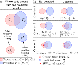
Figure 1: (a) Illustration for the two segmentation metrics false positive volume (FPV) and false negative volume (FNV). (b) Illustration for defining a true positive detection via three criteria, as explained in Section 3.4.2.

3.4.2 Detection metrics

Apart from the segmentation metrics discussed above, we also assessed the performance of our models on the test sets via three detection-based metrics for evaluating the detectibility of individual lesions within a patient.

In Criterion 1, a predicted lesion $P_{l^{\prime}}$ was labeled as true positive (TP) if at least one of $|G_{l}\cap P_{l^{\prime}}|>0$ for $l\in\{1,2,...,L_{g}\}$, otherwise $P_{l^{\prime}}$ was labeled as a false positive (FP). Similarly, a ground truth lesion $G_{l}$ was labeled as false negative (FN), if $|G_{l}\cap P_{l^{\prime}}|=0$ for all $l^{\prime}\in\{1,2,...,L_{p}\}$. This definition is a weak detection criterion, where any predicted lesion is considered TP by having just one of its voxels overlap with any ground truth lesion. In Criterion 2, all predicted lesions were first matched to their corresponding ground truth lesions by maximizing the IoU between each predicted and ground truth lesion pair. For a predicted lesion $P_{l^{\prime}}$ matched to a ground truth lesion $G_{l}$, $P_{l^{\prime}}$ was labeled as TP if $\frac{|G_{l}\cap P_{l^{\prime}}|}{|G_{l}\cup P_{l^{\prime}}|}\geq T$, and as FP if $0\leq\frac{|G_{l}\cap P_{l^{\prime}}|}{|G_{l}\cup P_{l^{\prime}}|}<T$, where the threshold $T=0.5$. This was a stronger detection criterion than Criterion 1 as it required the matching of ground truth and predicted lesions and also imposed IoU $>$ 0.5 condition. Lastly, in Criterion 3, all predicted and ground truth lesions were matched by maximizing IoU. For a matched pair $P_{l^{\prime}}$ and $G_{l}$, the lesion $P_{l^{\prime}}$ was labeled as TP if $|G_{l,\text{SUV}_{\text{max}}}\cap P_{l^{\prime}}|>0$, otherwise it was labeled as FP, where $G_{l,\text{SUV}_{\text{max}}}$ is the voxel in $G_{l}$ with the maximum SUV from the corresponding PET image. Hence, this detection criterion results in higher sensitivity upon segmenting the $\text{SUV}_{\text{max}}$ voxel of the ground truth lesions. For both Criteria 2 and 3, a ground truth lesion that was not matched with any of the predicted lesions based on IoU maximization was labeled as FN, while a predicted lesion not matched with any ground truth lesion was labeled as FP.

Although the definitions for detection metrics FP and FN might appear similar to the segmentation metrics FPV and FNV, on careful investigation, they are not (Fig. 1 (a) and (b)). FPV and FNV metrics compute the sum of the volumes of all lesions that are predicted in an entirely wrong location (no overlap with ground truth lesions) or lesions that are entirely missed, respectively. Hence, these metrics are defined at the voxel level for each patient. On the other hand, the detection metrics (in Criteria 1, 2, and 3) are defined on a per-lesion basis for each patient.

3.4.3 Inter-observer variability metrics

To quantify the inter-observer variability (Section 4.4), we used Fleiss’s kappa coefficient adapted for segmentation in a voxel-level binary classification manner [21]. Each voxel in an image (with $M$ voxels) was considered as a subject which were annotated by $N_{\text{obs}}$ observers, who assigned these voxels into one of $K_{\text{labels}}$. In our case, $N_{\text{obs}}=3$ and $K_{\text{labels}}=2$ (0 for background and 1 for lesion). The Fleiss’ kappa coefficient $\kappa$ for an image can then be written as a function of observed agreement $\bar{P}$, and the agreement by chance $\bar{P}_{e}$, as

$$\kappa=\frac{\bar{P}-\bar{P}_{e}}{1-\bar{P}_{e}}$$ (2)

where $\bar{P}$ is given by,

$$\bar{P}=\frac{1}{MN_{\text{obs}}(N_{\text{obs}}-1)}\Bigg{(}\sum_{i=1}^{M}\sum_{j=1}^{K_{\text{labels}}}(n_{ij})^{2}-MN_{\text{obs}}\Bigg{)}$$ (3)

and $\bar{P}_{e}$ is given by,

$$\bar{P}_{e}=\frac{1}{M^{2}N_{\text{obs}}^{2}}\sum_{j=1}^{K_{\text{labels}}}\Bigg{(}\sum_{i=1}^{M}n_{ij}\Bigg{)}^{2}$$ (4)

Here, $n_{ij}$ represents the number of physicians who assigned the $i^{th}$ voxel to the $j^{th}$ label in the image. Finally, $\kappa$ is averaged over all cases to obtain $\kappa_{\text{mean}}$ quantifying the measure of inter-observer variability between physicians. $\kappa$ (or $\kappa_{\text{mean}}$) lies in the range [-1.00, 1.00] with values $<$ 0 indicating no agreement, and values in the range 0–0.20 as slight, 0.21–0.40 as fair, 0.41–0.60 as moderate, 0.61–0.80 as substantial, and 0.81–1.00 as almost perfect agreement.

3.4.4 Clinically-relevant lesion measures

In the context of evaluating medical image lesion segmentation algorithms, incorporation of clinically-relevant lesion measures provides a comprehensive assessment that extends beyond traditional segmentation-based metrics, such as DSC. While these standard metrics offer insights into the quality of the segmentation itself, they may not always directly align with the clinical significance of the segmentation outcomes [22, 23]. In this work, we computed the lesion measures such as the patient-level lesion $\text{SUV}_{\text{mean}}$, $\text{SUV}_{\text{max}}$, number of lesions, TMTV, TLG and lesion dissemination $\text{D}_{\text{max}}$ from the ground truth and predicted segmentation masks. We defined $\text{D}_{\text{max}}$ as the distance between the two farthest located foreground voxels in cm. These lesion measures are particularly crucial in PET/CT-based lesion segmentation owing to their prognostic value in patient outcomes [2, 23].

Assessing the reproducibility of these lesion measures enhances the confidence in the segmentation algorithm’s results. Therefore, we conducted paired Student’s $t$-test analyses to determine the disparity in the means of the distributions between the ground truth and predicted lesion measures (Section 4.1.1). Additionally, similar analyses were carried out to evaluate intra-observer variability, involving two annotations made by the same physician on the same set of cases (Section 4.3).

4 Results

4.1 Segmentation performance

		Cohorts (test set)
		Internal				External
Networks	Metrics	Overall	DLBCL-BCCV (19 scans)	PMBCL-BCCV (25 scans)	DLBCL-SMHS (44 scans)	AutoPET lymphoma (145 scans)
	DSC (mean) ($\uparrow$)	0.60 ± 0.34	0.56 ± 0.35	0.49 ± 0.42	0.68 ± 0.27	0.56 ± 0.27
	DSC ($\uparrow$)	0.74 [0.26, 0.87]	0.72 [0.24, 0.89]	0.74 [0.02, 0.9]	0.78 [0.55, 0.87]	0.66 [0.33, 0.77]
	FPV ($\downarrow$)	6.26 [0.68, 32.06]	6.95 [0.0, 36.55]	2.23 [0.13, 17.47]	8.71 [1.19, 34.1]	38.41 [15.86, 128.47]
UNet	FNV ($\downarrow$)	0.0 [0.0, 5.05]	2.04 [0.0, 4.82]	0.0 [0.0, 1.24]	0.85 [0.0, 10.81]	0.41 [0.0, 3.88]
	DSC (mean) ($\uparrow$)	0.60 ± 0.34	0.56 ± 0.37	0.51 ± 0.41	0.68 ± 0.27	0.58 ± 0.27
	DSC ($\uparrow$)	0.76 [0.27, 0.88]	0.71 [0.19, 0.9]	0.72 [0.01, 0.85]	0.78 [0.62, 0.87]	0.68 [0.4, 0.78]
	FPV ($\downarrow$)	4.55 [1.35, 31.51]	5.78 [0.61, 19.97]	2.15 [0.52, 7.18]	9.18 [2.08, 38.87]	21.46 [6.3, 66.44]
SegResNet	FNV ($\downarrow$)	0.0 [0.0, 7.55]	1.17 [0.0, 5.59]	0.0 [0.0, 6.3]	0.0 [0.0, 10.81]	0.5 [0.01, 3.88]
	DSC (mean) ($\uparrow$)	0.56 ± 0.33	0.52 ± 0.37	0.45 ± 0.40	0.65 ± 0.24	0.55 ± 0.27
	DSC ($\uparrow$)	0.68 [0.3, 0.84]	0.69 [0.16, 0.87]	0.39 [0.02, 0.79]	0.73 [0.54, 0.83]	0.64 [0.33, 0.78]
	FPV ($\downarrow$)	15.27 [3.27, 52.27]	12.43 [1.24, 44.9]	8.17 [2.39, 33.99]	18.36 [8.85, 78.23]	36.61 [13.61, 107.33]
DynUNet	FNV ($\downarrow$)	0.0 [0.0, 7.31]	0.09 [0.0, 8.32]	0.0 [0.0, 1.24]	0.0 [0.0, 11.4]	0.42 [0.0, 4.17]
	DSC (mean) ($\uparrow$)	0.57 ± 0.32	0.52 ± 0.35	0.46 ± 0.38	0.66 ± 0.24	0.53 ± 0.27
	DSC ($\uparrow$)	0.67 [0.4, 0.85]	0.48 [0.21, 0.89]	0.45 [0.01, 0.78]	0.75 [0.52, 0.85]	0.61 [0.33, 0.75]
	FPV ($\downarrow$)	15.74 [3.86, 44.2]	9.13 [3.19, 87.47]	9.0 [3.87, 19.21]	19.98 [7.85, 43.51]	58.26 [19.35, 145.88]
SwinUNETR	FNV ($\downarrow$)	0.0 [0.0, 4.65]	0.09 [0.0, 3.39]	0.0 [0.0, 1.24]	0.0 [0.0, 8.83]	0.58 [0.01, 3.52]

Table 2: Comparison of the four networks on the internal (both aggregated and segregated by data origins and lymphoma subtypes) and external test sets evaluated via median values of patient-level DSC, FPV (in ml), and FNV (in ml). All the median values have been reported along with their IQRs. The mean patient-level DSC values on the test sets are also reported with the corresponding standard deviations.

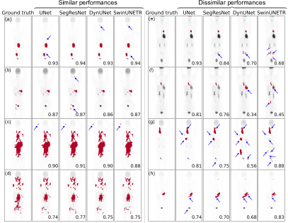
Figure 2: Visualization of performances of different networks on the coronal maximum intensity projection views for 8 representative cases. (a)-(d) show cases where all the networks had similar performances, while (e)-(h) show cases where the networks had dissimilar performances, often due to some of them predicting large FPVs. Some of the prominent FPVs have been indicated with blue arrows. The number on the bottom-right of each plot shows the DSC between the 3D predicted mask and the ground truth.

The performance of the four networks were evaluated using median DSC, FPV and FNV and mean DSC on both internal (including performances segregated by different internal cohorts) and external test sets, as shown in Table 2. Some visualization of networks performances have been illustrated in Fig. 2,

The SegResNet had the highest median DSC on both internal and external test sets with medians of 0.76 [0.27, 0.88] and 0.68 [0.40, 0.78], respectively. For the individual cohorts within the internal test set, UNet had the best DSC on both DLBCL-BCCV and PMBCL-BCCV with a median of 0.72 [0.24, 0.89] and 0.74 [0.02, 0.90], respectively, while SegResNet had the best DSC of 0.78 [0.62, 0.87] on DLBCL-SMHS. SegResNet also had the best FPV on both internal and external test sets with values of 4.55 [1.35, 31.51] ml and 21.46 [6.30, 66.44] ml. Despite the UNet winning on DSC for DLBCL-BCCV and PMBCL-BCCV sets, SegResNet had the best FPV on both these sets with median values of 5.78 [0.61, 19.97] ml and 2.15 [0.52, 7.18] ml, respectively, while UNet had the best FPV of 8.71 [1.19, 34.1] ml on DLBCL-SMHS. Finally, SwinUNETR had the best median FNV of 0.0 [0.0, 4.65] ml on the internal test set, while UNet had the best median FNV of 0.41 [0.0, 3.88] ml on the external test set. On DLBCL-BCCV and DLBCL-SMHS, SwinUNETR had the best median FNV of 0.09 [0.0, 3.39] ml and 0.0 [0.0, 8.83] ml, respectively, while on PMBCL-BCCV, UNet, DynUNet, and SwinUNETR were tied, each with a median value of 0.0 [0.0, 1.24] ml.

Firstly, both SegResNet and UNet generalized well on the unseen external test set, with a drop in mean & median performance by 4% & 8% and 2% & 8%, respectively as compared to the internal test set. Although the median DSC of DynUNet and SwinUNETR are considerably lower than SegResNet and UNet on the internal test set (by about 6-9%), these networks had even better generalizations with a drop in median DSC of only 4% and 6%, respectively, when going from internal to external testing. It is also worth noting that the DSC IQRs for all networks were larger on the internal test set as compared to the external test set. Also, all networks obtained a higher 75${}^{\text{th}}$ quantile DSC on the internal test set as compared to the external test set, while obtaining a lower 25${}^{\text{th}}$ quantile DSC on the internal test as compared to the external test set (except for SwinUNETR where this trend was reversed). Similarly, for different cohorts within the internal test set, all networks had the highest median and 25${}^{\text{th}}$ quantile DSC on DLBCL-SMHS set. The worst performance was obtained on the PMBCL-BCCV cohort with the largest IQR across all networks (see Section 4.1.2 and Fig. 6). Interestingly, despite having a lower performance on DSC on both internal and external test sets (as compared to the best performing models), SwinUNETR had the best median FNV values across cohorts in the internal test set.

4.1.1 Reproducibility of lesion measures

The lesion measures were computed at the patient level from the ground truth and the predicted masks for each of the networks on the internal and external test sets. The ground truth and predicted measures were compared via paired $t$-test at a significance level $\alpha=0.05$ with the null hypothesis stating that the true difference between their means is zero. To account for multiple testing (4 networks $\times$ 6 lesion measures), the value of $\alpha$ was adjusted via Bonferroni correction to $\alpha_{\text{corrected}}=\alpha/24=2.08\times 10^{-3}$, and all statistical tests were conducted using $\alpha_{\text{corrected}}$. Note that in these statistical tests, we desire that $p>\alpha_{\text{corrected}}$, meaning that the (null) hypothesis that there is indeed a statistically significant difference between the means of ground truth and predicted lesion measures shouldn’t be rejected, if our trained networks were performing ideally. Fig. 3 (a) shows that on the internal test set, $\text{SUV}_{\text{mean}}$ were reproducible ($p>\alpha_{\text{corrected}}$) by all networks except UNet, despite the UNet being one of our best performing models. Moreover, $\text{SUV}_{\text{max}}$ was not reproducible by any network except SegResNet (Fig. 3 (b)), number of lesions was only reproducible by UNet and SegResNet (Fig. 3 (c)), TMTV and TLG were reproducible by all networks (Fig. 3 (d)-(e)), and $\text{D}_{\text{max}}$ was not reproducible by any network (Fig. 3 (f)).

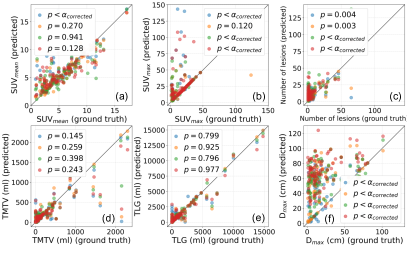
Figure 3: Predicted vs. ground truth lesion measures on the internal test set with $N_{\text{cases}}=88$. The reproducibility of clinically-relevant lesion measures was assessed for the four networks, UNet, SegResNet, DynUNet, and SwinUNETR via paired $t$-test. We desire $p>\alpha_{\text{corrected}}=2.08\times 10^{-3}$ (with Bonferroni correction to $\alpha=0.05$ for 24 tests) which denotes an absence of significant difference between the means of ground truth and predicted lesion measures. $\text{SUV}_{\text{mean}}$ was reproducible by all networks except UNet, $\text{SUV}_{\text{max}}$ by none except SegResNet, number of lesions by only UNet and SegResNet, TMTV and TLG by all networks, while $\text{D}_{\text{max}}$ by none of the networks.

Same analysis was carried out on the external test set, as shown in Fig. 4. For the external test set, the only lesion measures that were reproducible were $\text{SUV}_{\text{mean}}$ by SegResNet and SwinUNETR, number of lesions by SegResNet, and TLG by DynUNet. This shows that the performance of networks in terms of DSC or other traditional segmentation metrics don’t always reflect their adeptness at estimating lesion measures. Lesion measures such as $\text{SUV}_{\text{max}}$, number of lesions and $\text{D}_{\text{max}}$ are usually hard to reproduce by the networks. $\text{SUV}_{\text{max}}$ was highly sensitive to incorrect false positive predictions in regions of high SUV uptake. Similarly, the number of lesions were highly sensitive to incorrectly segmented disconnected components, and $\text{D}_{\text{max}}$ was highly sensitive to the presence of a false positive prediction far away from the ground truth segmentations (even though the volumes of such false positive predictions could be very small, in which case it would contribute very little to TMTV or TLG, as seen on the internal test set).

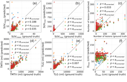
Figure 4: Predicted vs. ground truth lesion measures on the external test set with $N_{\text{cases}}=145$. The reproducibility of clinically-relevant lesion measures was assessed for the four networks, UNet, SegResNet, DynUNet, and SwinUNETR via paired $t$-test. We desire $p>\alpha_{\text{corrected}}=2.08\times 10^{-3}$ (with Bonferroni correction to $\alpha=0.05$ for 24 tests) which denotes an absence of significant difference between the means of ground truth and predicted lesion measures. Only reproducible quantities were $\text{SUV}_{\text{mean}}$ by SegResNet and SwinUNETR, number of lesions by SegResNet, and TLG by DynUNet.

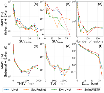
Figure 5: MAPE (%) as a function of ground truth lesion measures for the four networks, UNet, SegResNet, DynUNet, and SwinUNETR on the combined internal and external test set ($N_{\text{cases}}=233$). The percentage error in the network prediction of lesion measures, in general, decreases with increasing values of ground truth lesion measures. In particular, for $\text{SUV}_{\text{max}}$ (b), number of lesions (c), TMTV (d) and TLG (e) measures, MAPE plateaus for higher range of ground truth values.

To quantify the uncertainty in the prediction of lesion measures, we computed the Mean Absolute Percentage Error (MAPE) given by $100\times\frac{1}{N_{\text{cases}}}\sum_{i=1}^{N_{\text{cases}}}\big{|}\frac{b_{\text{pred}}-b_{\text{orig}}}{b_{\text{orig}}}\big{|}$, where $b_{\text{orig}}$ and $b_{\text{pred}}$ are the original and predicted values of lesion measures, respectively. The MAPE as a function of (ground truth) lesion measures on the combined internal and external test sets ($N_{\text{cases}}=233$) have been plotted in Fig. 5 (a)-(f). We utilized a combination of log-binning (for smaller values) and linear-binning (for larger values) of ground truth lesions measures to emphasize errors for small and large values, respectively. In general, the MAPE decreased as a function of ground truth lesion measures for all measures. In particular, for $\text{SUV}_{\text{max}}$, number of lesions, TMTV, and TLG measures (Fig. 5 (b)-(e)), MAPE also became (approximately) constant (averaged over all networks) at 53%, 44%, 31%, and 16% for values $\text{SUV}_{\text{max}}>17$, $L_{g}>60$, TMTV $>320$ ml, and TLG $>2500$ ml, respectively. The reduced error in the prediction of larger lesion measures also follows from our results in Fig. 7 in Section 4.1.2.

4.1.2 Effect of ground truth lesion measures values on network performance

First, we computed ground truth lesion measures for the internal and external test sets, and looked at the performance of UNet (based on DSC) for each of these measures and different datasets, as presented in Fig. 6. The performance was segregated into four different categories, namely (i) overall test set, (ii) cases with $\text{DSC}<0.2$, (iii) cases with $0.2\leq\text{DSC}\leq 0.75$, and (iv) cases with $\text{DSC}>0.75$ in the test set. From Fig. 6 (a)-(b), it is evident that for the categories with higher DSCs, the values of (mean and median) patient level $\text{SUV}_{\text{mean}}$ and $\text{SUV}_{\text{mean}}$ were also higher for internal cohort as well as the external cohort test sets. The lower overall performance on the PMBCL-BCCV set can also be attributed to lower overall mean and median $\text{SUV}_{\text{mean}}$ and $\text{SUV}_{\text{mean}}$. A similar trend was observed for number of lesion (Fig. 6 (c)) only on the external test set, but not on any of the internal test cohorts. Note that the mean number of lesions on the external test set was considerably higher than any of the internal test sets. For TMTV and TLG, all the cohorts with higher DSCs also had higher mean and median TMTVs or TLGs, except on the DLBCL-SMHS cohort, where the category $\text{DSC}<0.2$ had the highest mean and median TMTV and TLG. This anomaly can be attributed to the fact that despite being large, the lesions for cases in this category for this cohort were faint, as shown in Fig. 6 (a)-(b). Finally, for $\text{D}_{\text{max}}$, the category $0.2\leq\text{DSC}\leq 0.75$ had the highest median $\text{D}_{\text{max}}$ on all cohorts and highest mean $\text{D}_{\text{max}}$ on all cohorts except on DLBCL-SMHS. Lower values of $\text{D}_{\text{max}}$ signify lower spread of the disease, which can either correspond to cases with just one small lesion, or several (small or large) lesions located nearby.

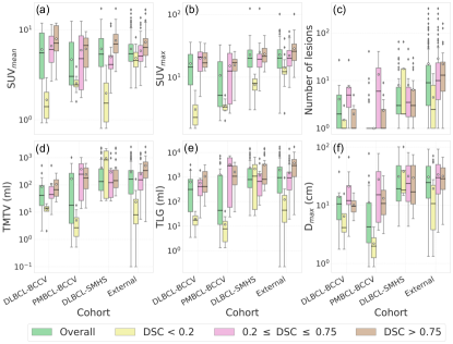
Figure 6: UNet performance (DSC) variations for different ground truth lesion measures on different test sets. For each test set, the lesion measure distributions have been presented as boxplots in four different categories, (i) on the overall test set, (ii) on cases with $\text{DSC}<0.2$, (iii) $0.2\leq\text{DSC}\leq 0.75$, and (iv) $\text{DSC}>0.75$. The $y$-axes for all the plots are in log scale, and the mean and median values for each box have been represented as white circles and black horizontal lines, respectively.

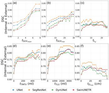
Figure 7: The effect of lesion measure values from subsets of test cases (internal and external combined with $N_{\text{cases}}=233$) on network performance. For a lesion measure $b$, a threshold $t_{b}$ was chosen and a subset of internal test cases were selected with $b\geq t_{b}$ and median DSC was computed on this subset. The value of $t_{b}$ were chosen in the range $[\mathcal{B}_{0},\mathcal{B}_{85}]$ at steps of $\Delta t_{b}$, where $\mathcal{B}_{0}$ and $\mathcal{B}_{85}$ represent the 0${}^{\text{th}}$ and 85${}^{\text{th}}$ quantile of the set of all lesion measures on the internal test set, $\mathcal{B}=\{b_{i}\}_{i=1}^{N_{\text{cases}}}$. (a), (b), (d), and (e) show that, in general, the performance of networks increase on subset with larger values of $\text{SUV}_{\text{mean}}$, $\text{SUV}_{\text{max}}$, TMTV, and TLG, respectively up to certain values of $t_{b}$ (after which the performance plateaus), while for the number of lesions (c) and $\text{D}_{\text{max}}$ (e) this increase isn’t very prominent.

Secondly, we evaluated the performance (median DSC) of the four networks on subsets of the combined internal and external test sets. Let the set $\mathcal{B}$ of patient level ground truth lesion measure $b$ on the test set be represented by $\mathcal{B}\mathrel{\mathop{:}}=\{b_{i}\}_{i=1}^{N_{\text{cases}}}$, where $N_{\text{cases}}=233$ is the total number of cases in the combined test set and $i$ denotes the case index. For a specific lesion measure $b$, subsets $\mathcal{B}_{\text{sub}}(t_{b})$ of the test cases were created by selecting a threshold $t_{b}$ such that $\mathcal{B}_{\text{sub}}\mathrel{\mathop{:}}=\{b_{i}|b_{i}\geq t_{b}\}$. For each value of $t_{b}$, median DSC was only evaluated on the subset of total test cases given by $\{i|b_{i}\geq t_{b}\}$. The values of $t_{b}$ were chosen in the range $\mathcal{B}_{0}\leq t_{b}\leq\mathcal{B}_{85}$ with a step-size of $\Delta t_{b}$, where $\mathcal{B}_{0}=\text{min}(\mathcal{B})$ and $\mathcal{B}_{85}$ respectively represent the 0${}^{\text{th}}$ quantile (i.e. the minimum) and the 85${}^{\text{th}}$ quantile of the set $\mathcal{B}$. The value of $\Delta t_{b}$ (chosen appropriately based on the range of values for a specific lesion measure) for $\text{SUV}_{\text{mean}}$, $\text{SUV}_{\text{max}}$, number of (ground truth) lesions ($L_{g}$), TMTV, TLG, and $\text{D}_{\text{max}}$ were chosen to be 1, 2, 1, 25 ml, 150 ml, and 3 cm, respectively.

The above analyses were performed for each biomarker and the results have been presented in Fig. 7. For the patient level $\text{SUV}_{\text{mean}}$, the median DSC increases monotonically as a function of $t_{\text{SUV}_{\text{mean}}}$ for all networks up to $t_{\text{SUV}_{\text{mean}}}\approx 6$, while for $t_{\text{SUV}_{\text{mean}}}>6$, the median DSC nearly plateaus (Fig. 7 (a)). The increase in median DSC up to $t_{\text{SUV}_{\text{mean}}}\approx 6$ is quite prominent, with an overall increase of about 13%, 14%, 14%, and 16% for UNet, SegResNet, DynUNet, and SwinUNETR, respectively. Also, as a function of $t_{\text{SUV}_{\text{mean}}}$, SegResNet had the best performance followed by UNet and other networks. DynUNet had better performance than SwinUNETR up to $t_{\text{SUV}_{\text{mean}}}\approx 5.5$ after which the trend between these two networks got switched. From these analyses, it can be concluded that the networks are more likely to segment lesions accurately and return a higher median DSC on a set of cases with higher ground truth $\text{SUV}_{\text{mean}}$ values.

A similar trend was observed for $\text{SUV}_{\text{max}}$, where for all networks, the median DSC increased up to $t_{\text{SUV}_{\text{max}}}\approx 30$ with SegResNet performing the best, followed by UNet. Just like for $\text{SUV}_{\text{mean}}$ measure, DynUNet performed better than SwinUNETR up to $t_{\text{SUV}_{\text{max}}}\approx 15$ after which their performances got switched. The networks had an overall increase of about 10%, 8%, 10%, and 12%, respectively (Fig. 7 (b)). This shows that a higher $\text{SUV}_{\text{max}}$ also, in general, leads to better segmentation performance. For the number of lesions, there was no significant increase (all networks $<5$%) as a function of $t_{L_{g}}$, while for $\text{D}_{\text{max}}$, there was a slight initial increase (up to $t_{\text{D}_{\text{max}}}\approx 20\text{ cm}$) but overall decrease later of 9%, 12%, 8%, and 6% for the networks, respectively. This suggests that while the number of lesions has no effect on performance, an increase in $\text{D}_{\text{max}}$ actually hurts the segmentation performance (Fig. 7 (c) and (f)). The median DSC also had considerable increase of 12%, 12%, 14%, and 14% for the networks respectively as a function of $t_{\text{TMTV}}$ with SegResNet and UNet with overlapping performances followed by DynUNet and SwinUNETR (Fig. 7 (d)), signifying that larger lesions are in general easier to segment accurately. Finally, a similar increase (up to $t_{\text{TLG}}\approx 2000\text{ ml}$) and plateauing behavior in median DSC was observed for the biomarker TLG with an overall increase of about 15%, 15%, 16%, and 18% respectively for these networks, meaning that metabolically active large lesions are much easier to segment as compared metabolically faint or smaller lesions (Fig. 7 (e)).

4.2 Detection performance

We evaluated the performance of our networks on three types of detection metrics, as defined in Section 3.4.2. Criterion 1, being the weakest detection criterion, had the best overall detection sensitivity of all criteria across all networks on both internal and external test sets, followed by Criterion 3 and then Criterion 2 (Fig. 8). From Criterion 1, UNet, SegResNet, DynUNet, and SwinUNETR obtained median sensitivities of 1.0 [0.57, 1.0], 1.0 [0.59, 1.0], 1.0 [0.63, 1.0], and 1.0 [0.66, 1.0] respectively on the internal test set, while on the external set, they obtained 0.67 [0.5, 1.0], 0.68 [0.51, 0.89], 0.70 [0.5, 1.0], and 0.67 [0.5, 0.86] respectively. Naturally, there was a drop in performance upon going from the internal to external testing. Furthermore, Criterion 1 had the best performance on the number of FP metrics with the networks obtaining 4.0 [1.0, 6.0], 3.0 [2.0, 6.0], 5.0 [2.0, 10.0], and 7.0 [3.0, 11.25] median FPs respectively on the internal test set, and 16.0 [9.0, 24.0], 10.0 [7.0, 19.0], 18.0 [10.0, 29.0], and 31.0 [21.0, 55.0] median FPs respectively on the external test set.

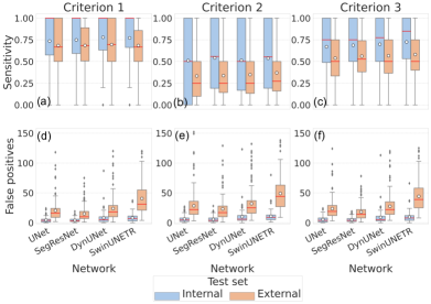
Figure 8: Median detection sensitivity and FP per patient via the three detection criteria for the four networks on the internal and external test sets. The top and bottom edges of the boxes span the IQR, while the red horizontal lines and white circles represent the median and mean respectively. The whiskers length is set to 1.5 times IQR and the outliers have been shown as black diamonds.

Furthermore, being a harder detection criterion, Criterion 2 had the lowest detection sensitivities for all networks with median being 0.5 [0.0, 1.0], 0.56 [0.19, 1.0], 0.5 [0.17, 1.0], and 0.55 [0.19, 1.0] respectively on the internal test set, and 0.25 [0.1, 0.5], 0.25 [0.14, 0.5], 0.25 [0.13, 0.5], and 0.27 [0.16, 0.5] respectively on the external test set. For this criterion, the drop in median sensitivities on going from the internal to external test set is comparable to those of Criterion 1. Similarly, for this criterion, the median FPs per patient were 4.5 [2.0, 8.0], 4.0 [2.0, 8.0], 6.0 [4.0, 12.25], and 9.0 [5.0, 13.0] respectively on the internal test set, and 22.0 [14.0, 36.0], 17.0 [10.0, 28.0], 25.0 [16.0, 37.0], and 44.0 [27.0, 63.0] respectively on the external test set. Despite the sensitivities being lower than in Criterion 1, the FPs per patient is similar on both internal and external test sets for Criterion 2 (although the variation of median FPs between criteria on the external test set for SwinUNETR is the highest).

Finally, the Criterion 3, based on the detection of the $\text{SUV}_{\text{max}}$ voxel of the lesions, was an intermediate criterion between Criteria 1 and 2, since the model’s ability to detect lesions accurately increases with the lesion $\text{SUV}_{\text{max}}$ (Section 4.1.2). For this criteria, the networks had median sensitivities of 0.75 [0.49, 1.0], 0.75 [0.5, 1.0], 0.78 [0.5, 1.0], and 0.85 [0.53, 1.0] respectively on the internal test set, and 0.5 [0.33, 0.75], 0.53 [0.38, 0.74], 0.5 [0.37, 0.75], and 0.5 [0.4, 0.75] respectively on the external test set. The drop in sensitivities between internal and external test sets is comparable to the other two criteria. Similarly, the networks had median FP per patient of 4.0 [1.0, 8.0], 4.0 [2.0, 7.0], 5.0 [3.0, 11.0], and 8.0 [4.0, 12.0] respectively on the internal test set, and 19.0 [12.0, 29.0], 14.0 [8.0, 22.0], 22.0 [14.0, 35.0], and 39.0 [25.0, 58.0] respectively on the external test set.

4.3 Intra-observer variability

To perform intra-observer variability analysis, 60 cases from the entire PMBCL-BCCV cohort (encompassing train, valid, and test sets) were re-segmented by Physician 4. This subset comprised of 35 “easy” cases (cases with UNet predicted masks obtaining $\text{DSC}>0.75$ with the original ground truth) and 25 “hard” cases ($\text{DSC}<0.2$). To eliminate bias, the selection of these cases, except for the DSC criteria, was randomized, ensuring no preference in the selection of specific cases were given during the re-segmentation process.

The overall mean and median DSC between physician’s original and new segmentations over the “easy” and “hard” cases combined was $0.50\pm 0.33$ and 0.49 [0.20, 0.84]. Here, the mean was comparable to the PMBCL-BCCV test set performance ($0.49\pm 0.42$) of UNet, although the median was much lower than that of UNet (0.74 [0.02, 0.9]). The “hard” cases exhibited lower reproducibility in generating consistent ground truth, as indicated by the mean and median DSCs between the original and re-segmented annotations, which were found to be $0.22\pm 0.18$ and 0.20 [0.05, 0.36] respectively. Conversely, for the “easy” cases, the mean and median DSC values were $0.70\pm 0.26$ and 0.82 [0.65, 0.87] respectively.

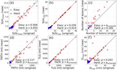
Figure 9: Quantifying the intra-observer (Physician 4) agreement for the reproducibility of lesion measures using paired $t$-test between the original and re-segmented (new) ground truth lesion measures. The significance level was chosen as $\alpha_{\text{corrected}}=8.33\times 10^{-3}$ (with Bonferroni correction for 6 tests). The analyses were performed on 60 cases from the PMBCL-BCCV cohort, with 35 cases classified as “easy” to segment by the UNet model ($\text{DSC}>0.75$ between the original ground truth and predicted masks,shown with red markers) and 25 cases classified as “hard” ($\text{DSC}<0.2$, shown with blue markers).

In addition, we assessed the reproducibility of lesion measures between the original and new segmentations via paired $t$-test, as illustrated in Fig. 9. At a Bonferroni corrected (for 6 tests of 6 lesion measures) significance level of $\alpha_{\text{corrected}}=8.33\times 10^{-3}$, all lesion measures were reproducible ($p>\alpha_{\text{corrected}}$) for the “easy“ cases except the number of lesions, while only $\text{SUV}_{\text{mean}}$, $\text{SUV}_{\text{max}}$, and number of lesions were reproducible for the “hard” cases. It is worth noting that the “easy” cases span a much larger range of lesion measures as compared to the “hard” cases (Fig. 9 (a)-(f)). As explained in Section 4.1.2, all networks were, in general, better at accurately delineating lesions (higher median DSC) on subset of cases with higher values of lesion measures. Physician 4 too was much more consistent with their ground truth delineation on the “easy” cases with larger values of lesion measures, as compared to the “hard” cases where the lesion measures had much lower values. Interestingly, the number of lesions measure was not reproducible on the “easy” cases, while it was on the “hard” cases, which reaffirms the fact that the physician was more consistent on this measure when there were lesser number of lesions to segment.

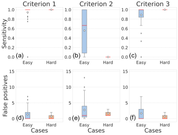
Figure 10: Assessing the intra-observer (Physician 4) variability using the three detection criteria on median sensitivity and FPs per patient metrics for the 35 “easy” and 25 “hard” cases from the PMBCL-BCCV cohort. For this analyses, the original segmentation by Physician 4 were treated as the ground truth and the new segmentations were treated as the predicted masks. The top and bottom edges of the boxes span the IQR, while the red horizontal lines and white circles represent the median and mean respectively. The whiskers length is set to 1.5 times IQR and the outliers have been shown as black diamonds.

Finally, we also performed detection analysis on the original and new segmentation, as illustrated in Fig. 10. For this analysis, we treated the original segmentation as ground truth and the new segmentation as predicted masks. For Criterion 1, the median detection sensitivities on both the “easy” and “hard” cases were 1.0 [1.0, 1.0], stating that the physician always segmented at least one voxel consistently between the original and new annotations. This criterion had median FPs per patient of 0.0 [0.0, 2.0] and 0.0 [0.0, 0.0] on the “easy” and “hard” cases respectively, stating that for the “hard” cases, the physician never segmented any lesion in an entirely different location as compared to their original masks. For Criterion 2, the sensitivities were 0.67 [0.08, 1.0] and 0.0 [0.0, 0.0] on the “easy” and “hard” cases respectively. This means that for the new annotation on the “hard” cases, the physician never segmented any lesion which had an IoU $>$ 0.5 with any lesions from the original annotation. For this criterion, the median FPs per patient were 1.0 [0.5, 4.0], and 1.0 [1.0, 1.0] for the “easy” and “hard” cases respectively. Finally, for Criterion 3, the sensitivities were 1.0 [0.84, 1.0] and 1.0 [0.5, 1.0], while the FPs per patient were 0.0 [0.0, 3.0] and 0.0 [0.0, 1.0] for the “easy” and “hard” cases respectively. It is worth noting that trend between the physician’s detection performance as assessed by these three criteria is similar to that by the four networks in Section 4.2 (Criterion 1 $>$ Criterion 3 $>$ Criterion 2).

4.4 Inter-observer variability

Nine cases (all belonging to different patients) were randomly selected from the DLBCL-BCCV set which were segmented by two additional physicians (Physicians 2 and 3). The mean Fleiss $\kappa$ coefficient over these 9 cases was 0.72, which falls in the category of “substantial” agreement between the physicians. This level of agreement underscores the reliability and consistency of the ground truth segmentation obtained from multiple annotators.

Secondly, we computed the pair-wise DSC between every two physicians for all 9 cases. The mean DSCs between Physicians 1 & 2, 2 & 3, and 1 & 3 were $0.67\pm 0.37$, $0.83\pm 0.20$, and $0.66\pm 0.37$. Moreover, the STAPLE [24] consensus for the three physicians were generated for all the 9 cases and DSCs between the STAPLE and ground truth segmentations were calculated for each physician. The mean DSCs with the STAPLE ground truth for Physicians 1, 2, and 3 were $0.75\pm 0.37$, $0.91\pm 0.11$, and $0.90\pm 0.16$, respectively.

5 Discussion

In this work, we trained and evaluated four distinct neural network architectures to automate the segmentation of lymphoma lesions from PET/CT datasets sourced from three different cohorts. To assess models performance, we conducted comprehensive evaluations on internal test set originating from these three cohorts and showed that SegResNet and UNet outperformed DynUNet and SwinUNETR on the DSC (mean and median) and median FPV metrics, while SwinUNETR had the best median FNV. In addition to internal evaluations, we extended our analysis to encompass an external out-of-distribution testing phase on a sizable public lymphoma PET/CT dataset. On this external test set as well, SegResNet emerged as the top performer in terms of DSC and FPV metrics, underscoring its robustness and effectiveness, while UNet displayed the best performance on FNV.

It is important to highlight that SegResNet and UNet were trained on patches of larger sizes, specifically (224, 224, 224) and (192, 192, 192) respectively, while DynUNet and SwinUNETR were trained using relatively smaller patches, namely (160, 160, 160) and (128, 128, 128) respectively. Utilizing larger patch sizes during training allows the neural networks to capture a more extensive contextual understanding of the data, thereby enhancing its performance in segmentation tasks [17]. This observation aligns with our results, where the superior performance of SegResNet and UNet can be attributed to their exposure to larger patch sizes during training. Moreover, larger batch sizes enable robust training by accurately estimating the gradients [17], but with our chosen training patch sizes, we could not train SegResNet, DynUNet and SwinUNETR with $n_{b}>1$ due to memory limitations (although we could accommodate $n_{b}=8$ for UNet). Hence, for a fair comparison between networks, all networks were trained with $n_{b}=1$. It is worth noting that our inability to train DynUNet and SwinUNETR on larger patch and mini-batch sizes was primarily due to computational resource limitations. However, this limitation presents an avenue for future research, where training these models with larger patches and batch sizes could potentially yield further improvements in segmentation accuracy.

We assessed the reproducibility of lesions measures and found that on the internal test set, TMTV and TLG were reproducible across all networks, while Dmax was not reproducible by any network. SUVmean was reproducible by all networks except UNet, SUVmax by only SegResNet and number of lesions by only UNet and SegResNet. On the external test set, reproducibility was more limited, with only SUVmean being reproducible by both SegResNet and SwinUNETR, number of lesions by SegResNet, and TLG by DynUNet (Fig. 3 and 4). Furthermore, we quantified the networks’ error in estimating the value of lesion measures using MAPE and found that MAPE generally decreases as a function of lesion measure values (for all lesion measures) on the combined internal and external test set (Fig. 5). The networks generally made significant errors in the accurate prediction when the ground truth lesion measures were very small. We also showed that, in general, on a set of images with larger patient level lesion $\text{SUV}_{\text{mean}}$, $\text{SUV}_{\text{mean}}$, TMTV, and TLG, a network is able to predict a higher median DSC, although for very high values of these lesion measures, the performance generally plateaus. On the other hand, the DSC performance is not much affected by the number of lesions, while for a set of images with higher $\text{D}_{\text{max}}$, the performance generally decreases for all networks (Fig. 7).

As much of PET/CT data is privately owned by healthcare institutions, it poses significant challenges for researchers in accessing diverse datasets for training and testing deep learning models. In such a scenario, to improve the interpretability of models, it is crucial for researchers to investigate how the performance of their models depend on dataset characteristics. By studying how model performance correlates with the image/lesion characteristics, researchers can gain insights into the strengths and limitations of their models [13].

Alongside the evaluation of segmentation performance, we also introduced three distinct detection criteria, denoted as Criterion 1, 2, and 3. These criteria served a specific purpose: to evaluate the networks’ performance on a per-lesion basis. This stands in contrast to the segmentation performance assessment, which primarily focuses on the voxel-level accuracy of the networks. The rationale behind introducing these detection criteria lies in the need to assess how well the networks identify and detect lesions within the images, as opposed to merely evaluating their ability to delineate lesion boundaries at the voxel level. The ability to detect the presence of lesions (Criterion 1) is crucial, as it directly influences whether a potential health concern is identified or missed. Detecting even a single voxel of a lesion could trigger further investigation or treatment planning. Lesion count and accurate localization (Criterion 2) are important for treatment planning and monitoring disease progression. Knowing not only that a lesion exists but also how many there are and where they are located can significantly impact therapeutic decisions. Criterion 3 which focused on segmenting lesions based on lesion metabolic characteristics ($\text{SUV}_{\text{max}}$), adds an additional layer of clinical relevance.

Using these detection metrics, we assessed the sensitivities and FP detections for all networks and showed that depending on the detection criteria, a network can have very high sensitivity even when the DSC performance was low. Given these different detection criteria, a trained model can be chosen based on specific clinical use cases. For example, some use cases might involve being able to detect all lesions without being overly cautious about segmenting exact lesion boundary, while some other use cases might be looking for more robust boundary delineations.

Furthermore, we assessed the intra-observer variability of a physician in segmenting both “easy” and “hard” cases, noting challenges in consistent segmentation of cases from the “hard” subset. In lymphoma lesion segmentation, cases can vary in difficulty due to factors like size, shape, and location of lesions, or image quality. By identifying which cases are consistently difficult for even an experienced physician to segment, we gained insights into the complexities and nuances of the segmentation task. Finally, we also assessed the inter-observer agreement between three physicians. Although, we inferred that there was substantial level of agreement between the three physicians, the assessment was performed only on 9 cases, resulting in low statistical power.

To improve the consistency of ground truth in medical image segmentation, a well-defined protocol is essential. This protocol should engage multiple expert physicians independently in delineating regions of interest (ROIs) or lesions within PET/CT images. Instead of a single physician segmenting a cohort independently, multiple annotators should segment the same images without knowledge of each other’s work. Discrepancies or disagreements among physicians can be resolved through structured approaches such as facilitated discussions, clinical information reviews, or image clarification. This robust ground truth process enhances inter-observer agreement accuracy and strengthens the validity of research findings and clinical applications relying on these annotations.

6 Conclusion

In this study, we assessed various neural network architectures for automating lymphoma lesion segmentation in PET/CT images across multiple datasets. We examined the reproducibility of lesion measures, revealing differences among networks, highlighting their suitability for specific clinical uses. Additionally, we introduced three lesion detection criteria to assess network performance at a per-lesion level, emphasizing their clinical relevance. Lastly, we discussed challenges related to ground truth consistency and stressed the importance of having well-defined protocol for segmentation. This work provides valuable insights into deep learning’s potentials and limitations in lymphoma lesion segmentation and emphasizes the need for standardized annotation practices to enhance research validity and clinical applications.

References

- [1] Sally F. Barrington et al. “FDG PET for therapy monitoring in Hodgkin and non-Hodgkin lymphomas” In European Journal of Nuclear Medicine and Molecular Imaging 44.1, 2017, pp. 97–110
- [2] Kursat Okuyucu et al. “Prognosis estimation under the light of metabolic tumor parameters on initial FDG-PET/CT in patients with primary extranodal lymphoma” In Radiol. Oncol. 50.4, 2016, pp. 360–369
- [3] Nan Wu et al. “Deep Neural Networks Improve Radiologists’ Performance in Breast Cancer Screening” In IEEE Transactions on Medical Imaging 39.4, 2020, pp. 1184–1194
- [4] Cheng Yuan et al. “Diffuse large B-cell lymphoma segmentation in PET-CT images via hybrid learning for feature fusion” In Medical Physics 48.7, 2021, pp. 3665–3678
- [5] Haigen Hu et al. “Lymphoma Segmentation in PET Images Based on Multi-view and Conv3D Fusion Strategy” In 2020 IEEE 17th International Symposium on Biomedical Imaging (ISBI), 2020, pp. 1197–1200
- [6] Haoming Li et al. “DenseX-Net: An End-to-End Model for Lymphoma Segmentation in Whole-Body PET/CT Images” In IEEE Access 8, 2020, pp. 8004–8018
- [7] Liangchen Liu et al. “Improved Multi-modal Patch Based Lymphoma Segmentation with Negative Sample Augmentation and Label Guidance on PET/CT Scans” In Multiscale Multimodal Medical Imaging Cham: Springer Nature Switzerland, 2022, pp. 121–129
- [8] Cláudia S. Constantino et al. “Evaluation of Semiautomatic and Deep Learning–Based Fully Automatic Segmentation Methods on [18F]FDG PET/CT Images from Patients with Lymphoma: Influence on Tumor Characterization” In Journal of Digital Imaging 36.4, 2023, pp. 1864–1876
- [9] Amy J. Weisman et al. “Comparison of 11 automated PET segmentation methods in lymphoma” In Physics in medicine & biology 65.23, 2020, pp. 235019–235019
- [10] Amy J. Weisman et al. “Convolutional Neural Networks for Automated PET/CT Detection of Diseased Lymph Node Burden in Patients with Lymphoma” In Radiology: Artificial Intelligence 2.5, 2020, pp. e200016
- [11] Chong Jiang et al. “Deep learning–based tumour segmentation and total metabolic tumour volume prediction in the prognosis of diffuse large B-cell lymphoma patients in 3D FDG-PET images” In European Radiology 32.7, 2022, pp. 4801–4812
- [12] Paul Blanc-Durand et al. “Fully automatic segmentation of diffuse large B cell lymphoma lesions on 3D FDG-PET/CT for total metabolic tumour volume prediction using a convolutional neural network.” In European Journal of Nuclear Medicine and Molecular Imaging 48.5, 2021, pp. 1362–1370
- [13] Shadab Ahamed et al. “A U-Net Convolutional Neural Network with Multiclass Dice Loss for Automated Segmentation of Tumors and Lymph Nodes from Head and Neck Cancer PET/CT Images” In Head and Neck Tumor Segmentation and Outcome Prediction Cham: Springer Nature Switzerland, 2023, pp. 94–106
- [14] Sergios Gatidis et al. “A whole-body FDG-PET/CT Dataset with manually annotated Tumor Lesions” In Scientific Data 9.1, 2022, pp. 601
- [15] Mihaela Pop et al. “Left-Ventricle Quantification Using Residual U-Net” 11395, Statistical Atlases and Computational Models of the Heart. Atrial Segmentation and LV Quantification Challenges Switzerland: Springer International Publishing AG, 2019, pp. 371–380
- [16] Andriy Myronenko “3D MRI Brain Tumor Segmentation Using Autoencoder Regularization”, Brainlesion: Glioma, Multiple Sclerosis, Stroke and Traumatic Brain Injuries Cham: Springer International Publishing, 2019, pp. 311–320
- [17] Fabian Isensee et al. “nnU-Net: a self-configuring method for deep learning-based biomedical image segmentation” In Nature Methods 18.2 Springer ScienceBusiness Media LLC, 2020, pp. 203–211
- [18] Ali Hatamizadeh et al. “Swin UNETR: Swin Transformers for Semantic Segmentation of Brain Tumors in MRI Images”, 2022
- [19] M. Cardoso et al. “MONAI: An open-source framework for deep learning in healthcare”, 2022 arXiv:2211.02701 [cs.LG]
- [20] Shadab Ahamed et al. “Towards enhanced lesion segmentation using a 3D neural network trained on multi-resolution cropped patches of lymphoma PET images” In Journal of Nuclear Medicine 64.supplement 1 Society of Nuclear Medicine, 2023, pp. P1360–P1360
- [21] Joseph L. Fleiss “Measuring nominal scale agreement among many raters” In Psychological bulletin 76.5, 1971, pp. 378–382
- [22] Abhinav K Jha et al. “Nuclear Medicine and artificial intelligence: Best practices for evaluation (the RELAINCE guidelines)” In J. Nucl. Med. 63.9 Society of Nuclear Medicine, 2022, pp. 1288–1299
- [23] Navid Hasani et al. “Artificial Intelligence in Lymphoma PET Imaging: A Scoping Review (Current Trends and Future Directions)” In PET clinics 17.1 Elsevier, 1, pp. 145–174
- [24] Simon K Warfield et al. “Simultaneous truth and performance level estimation (STAPLE): an algorithm for the validation of image segmentation” In IEEE Trans. Med. Imaging 23.7 Institute of ElectricalElectronics Engineers (IEEE), 2004, pp. 903–921