Extended edge modes and disorder preservation of a symmetry-protected topological phase out-of-equilibrium

Abstract

The time evolution of topological systems is an active area of interest due to their expected applications in fault-tolerant quantum computing. Here, we analyze the dynamics of a non-interacting spinless fermion chain in its topological phase, quenched out-of-equilibrium by a Hamiltonian belonging to the same symmetry class. Due to particle-hole symmetry, the bulk properties of the system remain intact throughout its evolution. However, the boundary properties may be drastically altered, with the initially localized Majorana edge modes extending across the chain. Up to a timescale $t^{*}$, identified by area-law behavior of the entanglement entropy, these extended edge modes are an example of exotic effects in topological systems out-of-equilibrium. Further, whilst local disorder can be utilized to preserve localization and increase $t^{*}$, we still identify non-trivial dynamics in the Majorana polarization and Loschmidt echo.

Introduction.—Non-interacting symmetry-protected topological (SPT) phases of matter are classified by the ten-fold way [1, 2, 3, 4]: a classification scheme that uses discrete symmetries of the underlying Hamiltonian to quantify the potential topological phases. Whilst this is well celebrated, it does not capture the possible phases of systems out-of-equilibrium. In this setting, due to the unitarity of the time evolution operator, only particle-hole symmetry (PHS) is preserved. Therefore, non-equilibrium systems require a different classification scheme than the static system, even if the Hamiltonians describing the initial system and the quench possess the same symmetries [5]. This can have striking consequences for SPT phases out-of-equilibrium, where the presence and nature of edge excitations may be dynamically modified [6, 7, 8, 9, 10].

Unfortunately, probes for dynamical changes in a topological phase are not trivially inherited from the analysis of equilibrium phases. As an example, consider a quench of a topologically non-trivial system defined by initial Hamiltonian $H^{(i)}$ and time evolution operator $U(t)=e^{-iH^{(f)}t}$, where $H^{(f)}$ is the post-quench (final) Hamiltonian. The evolved system is described by the fictitious Hamiltonian $H_{\mathrm{fic}}(t)=U(t)H^{(i)}U^{\dagger}(t)$, such that the time evolved many-body state $\ket{\Psi(t)}=U(t)\ket{\Psi}$ is an eigenstate of $H_{\mathrm{fic}}(t)$. As $H^{(i)}$ and $H_{\mathrm{fic}}(t)$ share the same gapped spectrum, one can be continuously deformed into the other. Then, provided this is performed in a symmetry-preserving manner, they will also share the same bulk topological properties and thus a bulk topological invariant will no longer capture dynamical changes in $\ket{\Psi(t)}$. To resolve this, it has been shown that degeneracies in the many-body entanglement spectrum (ES), manifesting as zero modes in the single-particle ES [10, 5], may still be used to identify dynamical phase changes [11, 12, 13, 14, 15, 16, 17]. Further, it is suggested that there exists a time $t^{*}\sim N/\nu_{LR}$, which scales with the size of the system $N$ and the Lieb-Robinson velocity $\nu_{LR}$, beyond which the topology of the system becomes ill-defined [5].

In this letter, we expose non-trivial dynamics when $t<t^{*}$, which we use to identify a weak breakdown in bulk-boundary correspondence. We show that the inclusion of local disorder [18], relevant when considering imperfections in experimental setups [19, 20, 21], effectively modifies $\nu_{LR}$ and may be utilized to stabilize the system. To exemplify our result, we investigate the non-equilibrium behavior of a one-dimensional system initialized in a topological phase [22], where both $H^{(i)}$ and $H^{(f)}$ belong to the BDI symmetry class, identified by the presence of PHS, time-reversal (TRS) and chiral (ChS) symmetries [3]. Since the TRS and ChS symmetries are dynamically broken [10], the symmetry class post-quench relaxes from a BDI to a D classification. Moreover, we show that the non-equilibrium setting introduces further modifications to the system and establish a breakdown in SPT order when the entanglement entropy (EE) crosses over from area- to volume-law behavior [23, 24, 25].

Model.—We study a model of spinless fermions on a quantum wire consisting of $N$ sites with open (OBC) and periodic (PBC) boundary conditions, described by the Kitaev chain Hamiltonian [22],

$$H^{(\alpha)}= \sum_{j}\left[-J^{(\alpha)}c_{j}^{\dagger}c_{j+1}+\Delta^{(\alpha)}c_{j}c_{j+1}+\mathrm{h.c.}\right]$$

$$-\mu_{j}^{(\alpha)}\left[c_{j}^{\dagger}c_{j}-\tfrac{1}{2}\right],$$ (1)

with $c_{j}^{\dagger}$ and $c_{j}$ being the creation and annihilation operators respectively on site $j$. These operators obey the usual anti-commutation relations, $\{c_{i},~{}c_{j}\}=\{c_{i}^{\dagger},~{}c_{j}^{\dagger}\}=0$ and $\{c_{i},~{}c_{j}^{\dagger}\}=\delta_{ij}$, with $J^{(\alpha)}\geq 0$ the nearest-neighbor hopping amplitude, $\Delta^{(\alpha)}=e^{-i\theta}|\Delta^{(\alpha)}|$ the $p-$wave superconducting pairing amplitude, $\mu^{(\alpha)}_{j}$ the local chemical potential, and $\alpha\in(i,f)$ identifying the initial and post-quench parameters. Throughout, we employ energy and time units of $J^{(i)}$ and $\hbar/J^{(i)}$ respectively (henceforth setting $\hbar=1$). In the case of OBC we identify $c_{N+1}=0$, whereas for PBC we identify $c_{N+1}=c_{1}$.

To probe the dynamics of this system in the presence of disorder, we investigate the time evolution of single-particle states up to half-filling, initialized in the non-trivial topological phase $(J^{(i)},~{}\Delta^{(i)},~{}\mu^{(i)}_{j})=(1,~{}0.9,~{}0.2)$. In $H^{(f)}$, the chemical potential is modified by a local disorder $\mu^{(f)}_{j}=\mu^{(i)}+w_{j}$, where $w_{j}=U[-W,W]$ is a uniformly distributed random number with $W\geq 0$ [26]. We identify the impact of disorder by averaging over $100$ distinct realizations.

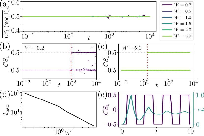
Figure 1: (a) Time evolution of $\overline{CS_{1}~{}(\mathrm{mod}~{}1)}$ for a chain with PBC and $N=180$. Quench parameters are $(J^{(f)},~{}\Delta^{(f)},~{}\mu_{j}^{(f)})=(J^{(i)},~{}0,~{}0.2+w_{j})$. (b, c) All realizations of $CS_{1}$ for two values of $W$. To resolve $CS_{1}$ with minimal noise, $5\times 10^{4}$ $k$-points are used for $W=5$ whilst $2\times 10^{5}$ are used for $W=0.2$. (d) $t_{\mathrm{osc}}$ with varying $W$, identified by red dashed lines in (b, c). (e) Left axis: Oscillations in the value of $CS_{1}$ for a single realization with $\mu_{j}^{(f)}=5$ for all $j$ (other values as above). Right axis: The corresponding rescaled return rate, $\tilde{L}$.

Topological analysis.—The Kitaev chain described by Eq. (Extended edge modes and disorder preservation of a symmetry-protected topological phase out-of-equilibrium) at equilibrium is classified by a bulk topological invariant $\nu_{BDI}\in\mathbb{Z}$, where $|\nu_{BDI}|$ identifies the number of exponentially localized Majorana zero-modes (MZMs) at either end of an open chain [4]. The non-trivial phases corresponding to $|\mu|<2J^{(i)}$ have invariants $\nu_{BDI}=\pm 1$ which, due to bulk-boundary correspondence, identifies a pair of chiral MZMs in each phase. Since the post-quench system lies within the D class, it instead is described by $\nu_{D}\in\mathbb{Z}_{2}$ [5].

To characterize the bulk topological phase of the system with PBC, we calculate the evolution of the one-dimensional Chern-Simons number [27, 3, 28, 10, 29],

$$CS_{1}(t)=\frac{1}{2\pi}\int_{BZ}dk\braket{\phi_{k}(t)}{\partial_{k}\phi_{k}(t)},$$ (2)

which is used to classify systems on one-dimensional manifolds [3]. Here, $\ket{\phi_{k}}$ are the instantaneous Bloch wavefunctions of the occupied bands, assumed to vary smoothly over the periodic 1D Brillouin zone. In the BDI class, $CS_{1}$ is quantized to non-zero half-integer values in the non-trivial phase and is related to the topological invariant via $\nu_{BDI}=2CS_{1}$. For the Kitaev chain, this is equivalent to the winding number [5]. Post-quench, the invariant becomes $\nu_{D}(t)=2\left(CS_{1}~{}\mathrm{mod}~{}1\right)$ since gauge transformations of $\ket{\phi_{k}}$ can modify the value of $CS_{1}$ by an integer [30, 28, 10]. The presence of disorder in $H^{(f)}$ breaks translational invariance, leaving the momentum-space representation ill-defined. However, the system can still be analyzed in terms of the pseudospin [11, 31, 32, 33] $\bm{n}(k,t)=\braket{\Phi^{\dagger}_{k}\bm{\sigma}\Phi_{k}}$, defined via the Fourier transformed spinor $\Phi_{i}=(c_{i},\,c^{\dagger}_{i})$, and may be extracted from the correlation matrix, $C$ (see Supplemental Material for further details [34]).

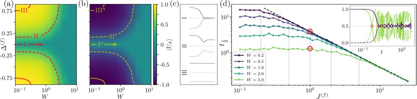
Figure 2: (a, b) The value to which $\braket{U_{S}}$ saturates at long time for the MZM initially localized at the left and right edges respectively. $W$ and $\Delta^{(f)}$ are varied, with other parameters the same as in Fig. 1. (c) Sketch of the realization-averaged Majorana subspecies amplitudes corresponding to contours in (a, b). $\tilde{n}_{e(o)}$ is represented by the solid (dashed) lines. (d) $t_{\frac{1}{2}}$ varying with $J^{(f)}$ for $\Delta^{(f)}=0$, other parameters are the same as in Fig. 1. The polynomial regime, proportional to $(J^{(f)})^{-1}$, is illustrated by the black dashed line. Inset: The Majorana distribution $n_{e(o)}$ for even (odd) subspecies, identified by solid (dashed) lines, for a single randomly selected realization with $W=0.5$ and $W=5$ at $J^{(f)}=1$.

Figure 1 (a) depicts $\overline{CS_{1}~{}\mathrm{mod}~{}1}$, the mean value of Eq. (2) modulo $1$ across all realizations. Although the constant value of $\overline{CS_{1}~{}\mathrm{mod}~{}1}$ indicates that the post-quench system remains in the non-trivial phase, other observables, such as the underlying pseudospin, still dynamically evolve. Indeed, the individual values of $CS_{1}$, though initially fixed to $-\nicefrac{{1}}{{2}}$ across all $W$, begin to oscillate between $\pm\nicefrac{{1}}{{2}}$ (see Figs. 1 (b, c)) after a characteristic time inversely proportional to the strength of the disorder, $\bar{t}_{\mathrm{osc}}\propto W^{-1}$ [34] (see Fig. 1 (d)). The frequency of these oscillations is not fixed in the presence of finite disorder, however they recover a regular period when disorder is removed (see Fig. 1 (e)). Opposite signs in $CS_{1}$ can be attributed to different phases in the static BDI system, but are topologically indistinct in the D class [34].

To further probe these oscillations we consider a system with OBC and determine the return rate $\tilde{L}(t)=-\nicefrac{{1}}{{N}}\log|L(t)|$ [12, 35], which exhibits peaks in its profile at times corresponding to Fisher zeros in the associated Loschmidt echo (LE) [36, 37, 38, 39, 40, 41], $L(t)=\braket{\Psi(0)}{U(t)}{\Psi(0)}$, when the system undergoes a dynamical phase change [39, 42, 13, 43]. The LE quantifies the revival of a quantum state during time evolution, as well as how sensitive the system dynamics are to quantum perturbations [38]. For a non-interacting system, the LE can also be determined from the correlation matrix $C$ [34]. In Fig. 1 (e) these signatures of dynamical phase transitions occur at the same rate as the oscillations in the associated $CS_{1}$ [44], suggesting that they can be attributed to revivals of the pre-quench topological phase. The strong correspondence between the pseudospin and LE dynamics, dictated by the presence of the MZMs on the open chain [41, 43], is less clear under the influence of disorder but can still be observed in the dynamics of the disordered system.

Polarization of MZMs.—Having identified the presence of non-trivial dynamics in the post-quench MZMs, we now probe the evolution of their chiral polarization. The pre-quench system possesses ChS, $U_{S}\mathcal{H}(t=0)U_{S}^{\dagger}=-\mathcal{H}(t=0)$, with $U_{S}$ representing the discrete symmetry operator anti-commuting with the first-quantized Hamiltonian $\mathcal{H}$, defined via $H_{\mathrm{fic}}(t)=\sum_{ij}\mathcal{H}_{ij}(t)\Phi_{i}^{\dagger}\Phi_{j}$. Initially, the MZMs are polarized with respect to ChS, in the sense that $\braket{\psi_{\pm}}{U_{S}}{\psi_{\pm}}=\pm 1$ for the two zero energy modes $\ket{\psi_{\pm}}$ . This relation no-longer strictly holds for $t>0$, yet one can still define the MZM polarization $\braket{U_{S}}_{\pm}(t)=\braket{\psi_{\pm}(t)}{U_{S}}{\psi_{\pm}(t)}$ for the time-evolved zero modes. We analyze the evolution of this quantity by varying both the final pairing amplitude, $\Delta^{(f)}$, and the disorder strength, $W$.

In the Majorana representation, the ChS operator is $U_{S}=\hat{1}_{N}\otimes\sigma_{z}$. Therefore the MZM polarization may be simply expressed as $\langle U_{S}\rangle(t)=\tilde{n}_{e}(t)-\tilde{n}_{o}(t)$ for a given single-particle state, where $\tilde{n}_{e(o)}(t)$ are the realization-averaged Majorana amplitudes over even (odd) Majorana sites. Figures 2 (a, b) show $\langle U_{S}\rangle$ at long time, identifying a competition between the protection of polarization for nonzero $\Delta^{(f)}$ and the suppression induced by $W$ for both the initially (a) left- and (b) right-localized MZMs. The profile of the corresponding Majorana populations broadly falls into the three regimes depicted in Fig. 2 (c), which illustrate how the realization-averaged even (solid line) and odd (dashed line) Majorana amplitudes vary with time. When $\Delta^{(f)}=0$, the average polarization decays within a finite time and lies in regime $I$. For a quench with nonzero $\Delta^{(f)}$, the MZMs retain their initial polarization either partially or fully, corresponding to the population profiles $II$ and $III$, respectively. However, the retention of polarization for $\Delta^{(f)}\neq 0$ diminishes as the magnitude of the disorder increases, with large enough $W$ forcing the polarization to relax to zero. The starred region labels in (b) correspond to states which have opposite polarization to those in (a), with regions identified in (c) indicated in (a,b).

Figure 2 (d) shows the value of $t_{\frac{1}{2}}$, the earliest time which satisfies $\tilde{n}_{e(o)}(t_{\frac{1}{2}})=0.5$, for $\Delta^{(f)}=0$ and varying $J^{(f)}$. This quantity can be used to characterize the polarization decay time. Two distinct regimes may be observed: one where $t_{\frac{1}{2}}$ is independent of the hopping amplitude, corresponding to $W\geq J^{(f)}$, and the second where $t_{\frac{1}{2}}\propto(J^{(f)})^{-1}$, corresponding to $W<J^{(f)}$. As with the profiles of $CS_{1}$, oscillations once again appear in individual realizations of $n_{e(o)}$. This is exemplified in the inset of Fig. 2 (d) for two values of $W$ at $\Delta^{(f)}=0$, where larger $W$ corresponds to an increased amplitude of oscillation. Moreover, the time at which these oscillations begin qualitatively exhibits the same $W$ dependence as $t_{\mathrm{osc}}$ (Fig. 1 (d)), highlighting another clear divergence from the static case where polarization is pinned to $\pm 1$. Next, we probe the system further through an investigation into its ES.

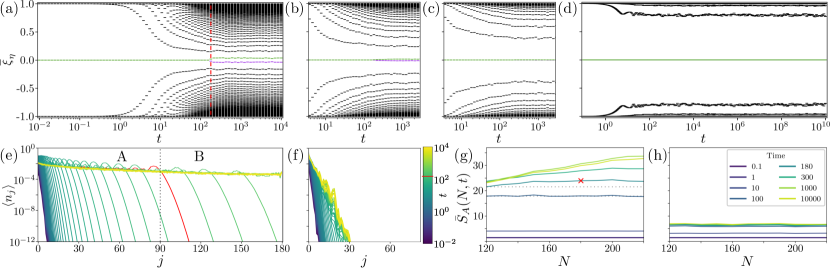
Figure 3: (a-d): Realization-averaged ES, $\bar{\xi}_{\eta}$, of the time-evolved states on a chain with OBC for disorder (a) $W=0.5$, (b) $W=1.0$, (c) $W=1.5$ and (d) $W=5.0$ (other parameters as in Fig. 1). (e, f) Time dynamics of the realization-averaged population profiles $\braket{n_{j}(t)}$ for the MZM initially localized at the left edge with (e) $W=0.5$ and (f) $W=5.0$. (g, h) Time cuts of the realisation-averaged EE, $\bar{S}_{A}$, scaling with the chain length, $N$, for bipartitions $N_{A}=N/2$ with (g) $W=0.5$ and (f) $W=1.5$. The red curve in (e) indicates the profile at $t\sim 180$, corresponding to the time at which the ES gap in (a) opens and a crossover from area-law to volume-law behavior in (g) may be observed.

Entanglement spectrum.—The ES is broadly used as a tool for categorizing topological systems [46, 47, 48, 11, 14] where a counting of degeneracies in the low-lying many-body ES is equivalent to a counting of MZMs localized at the boundaries in real space [46, 49, 50, 11]. Due to bulk-boundary correspondence, this degeneracy identifies a non-trivial topological invariant and is therefore indicative of a topological phase [46, 51, 52]. It has been suggested that in both the static and dynamical settings, the lifting of the many-body ES degeneracies can be interpreted as an indication of a topological phase transition [5]. For a non-interacting system, this is equivalent to identifying zeros in the single-particle ES [53, 54].

The single-particle ES, $\{\xi_{\eta}\}$, between subsystems $A$ and $B$ is found by diagonalizing $\Gamma=2C_{A}-I$, where $C_{A}=P_{A}CP_{A}$ is the reduced correlation matrix projected into the $A$ subsystem by $P_{A}$ [53, 54, 47]. Figures 3 (a-d) show the realization-averaged ES for a range of $W$, with $\Delta^{(f)}=0$ and a half-chain bipartition, $N_{A}=N/2$ . Evolving the system with $W>J^{(f)}$ (Figs. 3 (c, d)), we find that the ES exhibits bulk-boundary correspondence via the continued presence of the gapless zero-modes, indicating that it remains in a topologically non-trivial phase. On the other hand, for small disorder ($W{\leq}J^{(f)}$) the zero-mode degeneracy is lifted (Figs. 3 (a, b)). This would seem to indicate that the system has undergone a topological phase transition, which is in contradiction with the value of $\overline{CS_{1}~{}\mathrm{mod}~{}1}$ observed in Fig. 1 (a).

Localization profile.—To address what is happening to the MZMs as they evolve in time and to understand this contradiction, we calculate the realization-averaged contribution to the local fermion number, $\braket{n_{j}(t)}$, for the initially left-localized single-particle MZM . Figure 3 (e) shows that, for $\Delta^{(f)}=0$ and small $W$, the initially localized modes are driven to delocalize by the inter-site hopping, with a peak in the wavefront traveling along the chain. The time at which the ES zero-energy degeneracy is lifted (red dashed line in Fig. 3 (a)) corresponds to when the propagating peak in $\braket{n_{j}(t)}$ crosses the boundary between the $A$ and $B$ subdomains, leading to a finite entanglement.

By contrast, edge mode localization is preserved for large disorder (Fig. 3 (f)) and the ES zero modes remain gapless, well separated from the bulk ES modes throughout the time evolution. In both regimes, $\braket{n_{j}(t)}$ reaches a steady state after a finite time, with all profiles coinciding for times greater than $t\sim 10^{3}$. This is supported by the presence of zeros in the ES for the case of large $W$ when evaluated over a significantly longer time (see Fig. 3 (d)), which indicates that the profile shown in Fig. 3 (f) does not delocalize significantly further into the chain. Additionally, we note here that the features discussed above for $\Delta^{(f)}=0$ extend beyond this restricted regime, being tunable such that they are also present for $\Delta^{(f)}\neq 0$ [34].

Entanglement entropy.—As a final investigation into this system, we establish the regime for which the above analysis corresponds to a well-defined topological phase. An SPT phase is defined as a gapped, short-range entangled phase with a protecting symmetry [57, 4] and its EE should therefore exhibit area-law behavior [58, 25, 59]. In one dimension, this means that the EE is constant for $N_{A}\geq\lambda$, where $\lambda$ is the correlation length. Using this definition, we identify when SPT order becomes ill-defined through a crossover from area- to volume-law scaling, after which the EE will grow (linearly) with $N_{A}$. This crossover also defines the regime $t>t^{*}$ when the invariant no longer captures the topological phase of the time-evolved state.

The EE across the subdomain boundary can be determined directly from the corresponding ES via,

$$S_{A}=\sum_{\eta}\ln(1+e^{-\varepsilon_{\eta}})+\sum_{\eta}\frac{\varepsilon_{\eta}}{e^{\varepsilon_{\eta}}+1}$$ (3)

where $\varepsilon_{\eta}=2\operatorname{arctanh}(\xi_{\eta})$ are the spectrally flattened ES. Figures 3 (g, h) show how the realisation-averaged EE, $\bar{S}_{A}$ with $N_{A}=N/2$, scales with system size for small and large $W$, respectively. For small $W$, the EE profile exhibits a clear crossover from area- to volume-law behavior. This signals a breakdown in SPT order due to correlations spreading across the full length of the chain after sufficient time $t^{*}$ has elapsed. For the ES illustrated in Fig. 3 (a), this coincides with the time at which both the ES gap opens and the extended edge modes cross the subdomain boundary. However, for large $W$ the EE retains an area-law profile, indicating that the system remains short-range entangled and demonstrating that local disorder can be employed to stabilize SPT order.

Discussion.—In this work, we expose non-trivial dynamics that depend significantly upon the strength of the local disorder potential. Importantly, for small disorder such that correlations are free to spread throughout the system, we find that the initially localized modes will extend away from the edge until a time $t^{*}$. After this time, SPT order becomes ill-defined and the invariant can no longer faithfully describe the system. We identify the $t<t^{*}$ regime as one with a weak breakdown in bulk-boundary correspondence since the edge mode is no longer pinned to the boundary, but does retain an exponential profile and a finite correlation length. Our choice to partition the system equidistant from the left and right boundaries thus allows us to identify a maximum time for which SPT order is well-defined. An asymmetric partition will inevitably result in the ES gap opening and the area- to volume-law EE crossover occurring at an earlier time. However, for generic partitions sufficiently far from the edge, the system will maintain a regime for which there is a finite correlation length, well-defined topology, and extended edge modes. Additionally, it is possible to stabilize the topological phase by increasing the value of disorder and suppressing inter-site transport. In this regime, the value of $t^{*}$ is increased and the system maintains short-ranged entanglement throughout the time evolution. Yet, we still identify non-trivial dynamics in the polarization and Loschmidt echo corresponding to the preservation of chiral symmetry. In future work, we aim to extend the framework presented here to other non-interacting SPT phases [60], where the existence of multiple edge Majoranas is possible and we expect more exotic dynamical phase transitions to occur.

I Majorana representation

Here we summarize the treatment of the fermion chain using the Majorana representation. The Hamiltonian can be expressed in terms of Majorana fermion operators via the creation and annihilation operators, $c_{j}^{\dagger}=\frac{1}{2}(\gamma_{2j}+i\gamma_{2j+1})e^{i\theta/2}$ and $c_{j}=\frac{1}{2}(\gamma_{2j}-i\gamma_{2j+1})e^{-i\theta/2}$, where $\{\gamma_{j},\gamma_{k}\}=2\delta_{jk}$, $\gamma_{j}=\gamma_{j}^{\dagger}$ and ${(\gamma_{j})}^{2}=1$. By choosing $\theta=0$, $H^{(i/f)}$ given in Eq. (1) in the main text may be expressed as

$$H^{(\alpha)}= \frac{i}{2}\sum_{j}\gamma_{2j}\gamma_{2j+3}(J^{(\alpha)}-|\Delta^{(\alpha)}|)+\gamma_{2j+2}\gamma_{2j+1}(J^{(\alpha)}+|\Delta|^{(\alpha)})+\mu_{j}^{(\alpha)}\gamma_{2j}\gamma_{2j+1}=:\sum_{ij}\mathcal{H}^{(\alpha)}_{ij}\gamma_{i}\gamma_{j}.$$ (S1)

$H^{(\alpha)}$ is invariant under TRS, PHS and ChS, classifying it as a BDI class system. Thus there exist unitary matrices $U_{T}$, $U_{C}$ and $U_{S}$ such that $U_{T}(\mathcal{H}^{(\alpha)})^{*}U_{T}^{\dagger}=\mathcal{H}^{(\alpha)}$, $U_{C}(\mathcal{H}^{(\alpha)})^{*}U_{C}^{\dagger}=-\mathcal{H}^{(\alpha)}$ and $U_{S}\mathcal{H}^{(\alpha)}U_{S}^{\dagger}=-\mathcal{H}^{(\alpha)}$. In the Majorana basis, these matrices can be expressed as: $U_{T}=\hat{1}_{2N}$ and $U_{C}=U_{S}=\hat{1}_{N}\otimes\sigma_{z}$, resulting in operators for TRS, PHS and ChS represented by $T=U_{T}\mathcal{K}=\hat{1}_{2N}\mathcal{K}$, $C=\hat{1}_{N}\otimes\sigma_{z}\mathcal{K}$ and $S\equiv U_{S}=\hat{1}_{N}\otimes\sigma_{z}$, respectively, with $\mathcal{K}$ being element-wise complex conjugation. Using these relations, it is straightforward to show that $\mathcal{H}(t)$ respects PHS: $U_{C}\mathcal{H}(t)^{*}U_{C}=U_{C}e^{-it\left(\mathcal{H}^{(f)}\right)^{*}}U_{C}U_{C}\left(\mathcal{H}^{(i)}\right)^{*}U_{C}U_{C}e^{it\left(\mathcal{H}^{(f)}\right)^{*}}U_{C}=e^{it\mathcal{H}^{(f)}}\left(-\mathcal{H}^{(i)}\right)e^{-it\mathcal{H}^{(f)}}=-\mathcal{H}(t)$, where we used $U_{C}\left(\mathcal{H}^{(i/f)}\right)^{*}U_{C}=-\mathcal{H}^{(i/f)}$.

I.1 The correlation matrix in the Majorana representation

Throughout our numerical studies we extensively used the correlation matrix $C$, containing all quantum correlations of the system. This is given in the Majorana basis as follows: $C_{jk}(t)=\langle\left.\Psi(t)\right|\gamma_{j}\gamma_{k}\left|\Psi(t)\right.\rangle$, a $2N\times 2N$ matrix with the instantaneous (time-evolved initial) ground state $\ket{\Psi(t)}$. In the fermion basis, the single-particle correlations are given by the combinations $\mathcal{C}=\langle c^{\dagger}c\rangle$ and $\mathcal{F}=\langle cc\rangle$, two $N\times N$ matrices. In order to establish relations with the Majorana correlation matrix $C$, we consider the following expectation values:

$$\langle\gamma_{2i}\gamma_{2j}\rangle= \langle(c^{\dagger}_{i}+c_{i})(c^{\dagger}_{j}+c_{j})\rangle=\langle c^{\dagger}_{i}c^{\dagger}_{j}\rangle+\langle c_{i}c_{j}\rangle+\langle c^{\dagger}_{i}c_{j}\rangle+\langle c_{i}c^{\dagger}_{j}\rangle=\mathcal{F}^{*}_{ji}+\mathcal{F}_{ij}+\mathcal{C}_{ij}+\delta_{ij}-\mathcal{C}_{ji}$$

$$= \delta_{ij}+\mathcal{C}_{ij}-\mathcal{C}^{*}_{ij}+\mathcal{F}_{ij}-\mathcal{F}^{*}_{ij}=\delta_{ij}+2i\text{Im}\,\mathcal{C}_{ij}+2i\text{Im}\,\mathcal{F}_{ij}=:\delta_{ij}+i\Gamma_{2i,2j},$$ (S2)

$$\langle\gamma_{2i+1}\gamma_{2j+1}\rangle= \langle(-i)(c^{\dagger}_{i}-c_{i})(-i)(c^{\dagger}_{j}-c_{j})\rangle=-\langle c^{\dagger}_{i}c^{\dagger}_{j}\rangle-\langle c_{i}c_{j}\rangle+\langle c^{\dagger}_{i}c_{j}\rangle+\langle c_{i}c^{\dagger}_{j}\rangle=-\mathcal{F}^{*}_{ji}-\mathcal{F}_{ij}+\mathcal{C}_{ij}+\delta_{ij}-\mathcal{C}_{ji}$$

$$= \delta_{ij}+\mathcal{C}_{ij}-\mathcal{C}^{*}_{ij}-\mathcal{F}_{ij}+\mathcal{F}^{*}_{ij}=\delta_{ij}+2i\text{Im}\,\mathcal{C}_{ij}-2i\text{Im}\,\mathcal{F}_{ij}=:\delta_{ij}+i\Gamma_{2i+1,2j+1},$$ (S3)

$$\langle\gamma_{2i}\gamma_{2j+1}\rangle= \langle(c^{\dagger}_{i}+c_{i})(-i)(c^{\dagger}_{j}-c_{j})\rangle=-i\langle c^{\dagger}_{i}c^{\dagger}_{j}\rangle+i\langle c_{i}c_{j}\rangle+i\langle c^{\dagger}_{i}c_{j}\rangle-i\langle c_{i}c^{\dagger}_{j}\rangle=i\left(\mathcal{F}_{ij}-\mathcal{F}^{*}_{ji}+\mathcal{C}_{ij}-\delta_{ij}+\mathcal{C}_{ji}\right)$$

$$=-i\left(\delta_{ij}-\mathcal{C}_{ij}-\mathcal{C}^{*}_{ij}-\mathcal{F}_{ij}-\mathcal{F}^{*}_{ij}\right)=-i\left(\delta_{ij}-2\text{Re}\,\mathcal{C}_{ij}-2\text{Re}\,\mathcal{F}_{ij}\right)=:i\Gamma_{2i,2j+1},$$ (S4)

$$\langle\gamma_{2i+1}\gamma_{2j}\rangle= \langle\gamma_{2j}\gamma_{2i+1}\rangle^{*}=i\left(\delta_{ij}-\mathcal{C}^{*}_{ji}-\mathcal{C}_{ji}-\mathcal{F}^{*}_{ji}-\mathcal{F}_{ji}\right)=i\left(\delta_{ij}-\mathcal{C}_{ij}-\mathcal{C}^{*}_{ij}+\mathcal{F}_{ij}+\mathcal{F}^{*}_{ij}\right)$$

$$= i\left(\delta_{ij}-2\text{Re}\,\mathcal{C}_{ij}+2\text{Re}\,\mathcal{F}_{ij}\right)=:i\Gamma_{2i+1,2j},$$ (S5)

where $\langle\dots\rangle=\bra{\Psi(t)}\dots\ket{\Psi(t)}.$ Indices with different parity involve different combinations of the correlation matrix $\mathcal{C}_{ij}$ and $\mathcal{F}_{ij}$, as detailed above. It is possible to summarize the structure of the Majorana correlation matrix as follows: $C_{ij}=\langle\gamma_{i}\gamma_{j}\rangle=\delta_{ij}+i\Gamma_{ij}$, where using the anti-commutation relations give $2\delta_{ij}=\langle\gamma_{i}\gamma_{j}+\gamma_{j}\gamma_{i}\rangle=2\delta_{ij}+i\left(\Gamma_{ij}+\Gamma_{ji}\right)$, meaning that $\Gamma_{ij}$ is anti-symmetric.

In the $N\rightarrow\infty$ limit the midgap energy eigenstates are exactly degenerate, thus distinguishing which mode is populated at half-filling is ambiguous. To resolve this ambiguity we are free to take a linear combination of these states. For the system size simulated in this work, the states are sufficiently close to degenerate that this procedure is also necessary. Therefore, we construct a new state in the zero-energy subspace as a general linear combination of $\ket{\psi_{-}}$ and $\ket{\psi_{+}}$, the ‘lower’ and ‘upper’ zero modes respectively. This takes the form $\ket{\theta}=\cos(\theta)\ket{\psi_{-}}+\sin(\theta)\ket{\psi_{+}}$, where $\theta$ is an arbitrary phase. Elements of the correlation matrix in the zero-energy subspace are then given by the dyadic product, $C^{0}_{jk}(\theta)=\braket{\theta_{k}}{\theta_{j}}$. To account for all possible choices of $\theta$ we integrate over this manifold with an equal weight, $\frac{1}{2\pi}\int_{0}^{2\pi}d\theta C^{0}_{jk}=\frac{1}{2}(\braket{\psi_{-,k}}{\psi_{-,j}}+\braket{\psi_{+,k}}{\psi_{+,j}})$. As a consequence, cross-terms between $\ket{\psi_{-}}$ and $\ket{\psi_{+}}$ vanish, and we can include the zero modes in the correlation matrix of states up to half filling by simply summing over them (as in the definition for $C_{jk}$ in the main text) with an additional prefactor of $1/\sqrt{2}$.

II Dynamics of the pseudospin

II.1 Effective Bloch bands

Let us first look at periodic systems in order to introduce the tools we use to analyze the topological phase. In this case, the momentum space has a practical purpose of indexing the single-particle eigenstates of the system. By introducing the Fourier transformed fermionic operators

$$\widetilde{c}_{k}=\frac{1}{\sqrt{N}}\sum_{j}e^{ikj}c_{j}, \widetilde{c}^{\dagger}_{k}=\frac{1}{\sqrt{N}}\sum_{j}e^{-ikxj}c_{j}^{\dagger},$$ (S6)

the Hamiltonian can be written as a sum of $2\times 2$ matrices: $H^{(i/f)}=\sum_{k}\Phi^{\dagger}_{k}\widetilde{\mathcal{H}}^{(i/f)}(k)\Phi_{k}$, i.e. it is partially diagonalized by introducing the momentum space spinor field $\Phi_{k}=(\widetilde{c}_{k},\,\widetilde{c}^{\dagger}_{-k})$. For any $k$ in the Brillouin zone,

$$\widetilde{\mathcal{H}}(k)=d\left(\begin{array}[]{cc}n_{z}&n_{x}-in_{y}\\ n_{x}+in_{y}&-n_{z}\end{array}\right)=d\left(n_{x},\,n_{y},\,n_{z}\right)\cdot\bm{\sigma}\equiv\bm{d}(k)\cdot\bm{\sigma},$$ (S9)

where length $d=|\bm{d}|$ is the absolute value of the energy and $\bm{n}=\frac{\bm{d}}{d}$ is the pseudospin. There are two eigenvectors with energies $\pm d$, corresponding to the Bloch bands of particles and holes, respectively: $\bm{d}\cdot\bm{\sigma}\left|k,\pm\right>=\pm d\left|k,\pm\right>$:

$$\left|k,+\right>=\frac{1}{\sqrt{2(1+n_{z})}}\left(\begin{array}[]{c}1+n_{z}\\ n_{x}+in_{y}\end{array}\right), \left|k,-\right>=\frac{1}{\sqrt{2(1+n_{z})}}\left(\begin{array}[]{c}-n_{x}+in_{y}\\ 1+n_{z}\end{array}\right),$$ (S14)

which are orthogonal, so one can build the projectors to the upper and lower Bloch band, respectively: $\ket{k,\pm}\bra{k,\pm}=\frac{1}{2}\left(\hat{1}\pm\bm{n}(k)\cdot\bm{\sigma}\right)$. In order to follow the time-evolution of the pseudospin, we define the pseudospin operator in the Heisenberg picture as $\bm{s}(k,t)=e^{it\widetilde{\mathcal{H}}^{(f)}(k)}\bm{\sigma}e^{-it\widetilde{\mathcal{H}}^{(f)}(k)}$. Its expectation value with respect to a negative energy eigenstate of $\widetilde{\mathcal{H}}^{(i)}(k)$ with a given momentum $k$ gives $\left<k,-\right|\bm{s}(k,t)\left|k,-\right>=-\bm{n}(k,t)$. It is possible to derive a closed expression for the pseudospin by solving the differential equation $\partial_{t}\bm{n}(k,t)=2\bm{d}^{(f)}(k)\times\bm{n}(k,t)$ with the initial value $\bm{n}(k,t=0)=\bm{n}^{(i)}(k)$, which results in:

$$\bm{n}(k,t)= \cos\left(2|\bm{d}^{(f)}(k)|t\right)\bm{n}^{(i)}(k)+\sin\left(2|\bm{d}^{(f)}|t\right)\bm{n}^{(f)}\times\bm{n}^{(i)}+2\sin^{2}\left(|\bm{d}^{(f)}|t\right)\bm{n}^{(i)}\cdot\bm{n}^{(f)}\,\bm{n}^{(f)}.$$ (S15)

The pseudospin vectors corresponding to the pre- and post-quench Hamiltonians are defined as $\bm{n}^{(i/f)}(k):=\frac{\bm{d}^{(i/f)}(k)}{|\bm{d}^{(i/f)}(k)|}$, cf. Eq. S9. For illustration, let us assume the hopping, chemical potential and pairing amplitude in the initial and final systems to be $(J,\,0,\,\Delta)$ and $(J,\,W,\,0)$, respectively. The corresponding time-dependent pseudonspin texture then reads as follows:

$$\bm{n}(k,t)= \frac{-1}{\sqrt{J^{2}\cos^{2}k+\Delta^{2}\sin^{2}k}}\left(\begin{array}[]{c}\Delta\sin k\sin\left(2t(J\cos k+W)\right)\\ \Delta\sin k\cos\left(2t(J\cos k+W)\right)\\ J\cos k\end{array}\right).$$ (S19)

One can immediately see that $\bm{n}(k,t>0)$ is no longer restricted in the $yz-$plane as is the case for both $\bm{n}^{(i)}$ and $\bm{n}^{(f)}$. Later we will show how the pseudospin dynamics is reflected in the topological number for the initial BDI system, $\nu_{BDI}$.

Before turning to the definition of the topological numbers, let us discuss the role of pseudospin in a non-periodic system. The simplifications coming with the usual momentum space are lost in the non-periodic case, i.e. one needs two momenta to parameterize a quadratic Hamiltonian, since the energy does not only depend on the position difference of the spinors, but their actual position as well. Therefore one can define, analogously to the pseudospin operator, $\bm{\mathfrak{s}}(k,k^{\prime}):=\Phi^{\dagger}_{k}\bm{\sigma}\Phi_{k^{\prime}}$ by the Fourier transform of the following non-local coordinate space operator: $\bm{\mathfrak{s}}(x,x^{\prime}):=\Phi^{\dagger}(x)\bm{\sigma}\Phi(x^{\prime})$. To describe correlations between the coordinate points $x$ and $x^{\prime}$ one can use an ‘average’ position $X=\frac{x+x^{\prime}}{2}$ and a $y=x-x^{\prime}$ as the deviation from it. Fourier transform with respect to $y$ gives the ‘usual’ momentum variable in periodic systems, but now the resulting quantity still depends on the coordinate $X$. Let us note, that since $\langle\bm{\mathfrak{s}}(x,x^{\prime})\rangle$ is not assumed to be periodic, there is only one-to-one correspondence with the Fourier transformed and real space quantities in the infinite system size (or continuum) limit. Working with the Fourier transform of the generalized pseudospin:

$$\sum\limits_{y}e^{iky}\sum\limits_{X}\langle\bm{\mathfrak{s}}(X+y/2,X-y/2)\rangle=\frac{1}{N}\sum_{X,y}\sum_{q,q^{\prime}}e^{-iX(q-q^{\prime})+iy\left(k-\frac{q+q^{\prime}}{2}\right)}\langle\Phi^{\dagger}_{q}\bm{\sigma}\Phi_{q^{\prime}}\rangle=\langle\Phi^{\dagger}_{k}\bm{\sigma}\Phi_{k}\rangle\equiv-\bm{n}(k),$$ (S20)

where we assumed that in the initial state of the system all negative energy states are occupied. One realizes that $\bm{n}(k)$ is the spatial average of the local pseudospin $\bm{n}(X,k)=-\sum_{y}e^{iky}\langle\Phi^{\dagger}(X+\frac{y}{2})\bm{\sigma}\Phi(X-\frac{y}{2})\rangle$. Consequently, one can introduce the effective Bloch bands as the eigenvectors of the average pseudospin matrix: $\bm{n}(k)\cdot\bm{\sigma}=:\ket{k,+}\bra{k,+}-\ket{k,-}\bra{k,-}$. For a finite-size system this relationship is not exact, however, $\bm{n}$ is still a meaningful quantity, approximating the spatially averaged pseudospin of the system.

II.2 Pseudospin from the correlation matrix

As we have previously seen, the expectation value $\langle\Phi^{\dagger}_{k}(t)\bm{\sigma}\Phi_{k}(t)\rangle=-\bm{n}(k,t)$ gives the pseudospin texture. Here we express $\bm{n}$ with the help of the single-particle correlation functions. In order to do this, we write the expectation value of the pseudospin operator in terms of $\langle\widetilde{c}^{(\dagger)}_{k}(t)\widetilde{c}^{(\dagger)}_{-k}(t)\rangle$ and $\langle\widetilde{c}^{\dagger}_{k}(t)\widetilde{c}_{k}(t)\rangle$, then we relate it to the Majorana correlation matrix as well. Using the anti-commutation relations and manipulating the indices $i$ and $j$ we arrive at the manifestly real valued expressions:

$$n_{x}(k,t)= -\langle\Phi^{\dagger}_{k}(t)\sigma_{x}\Phi_{k}(t)\rangle=-\frac{1}{N}\sum_{ij}e^{-ik(x_{i}-x_{j})}\left(\langle c^{\dagger}_{i}(t)c^{\dagger}_{j}(t)\rangle+\langle c_{i}(t)c_{j}(t)\rangle\right)$$

$$= -\frac{1}{N}\sum_{ij}(-i)\sin(k(x_{i}-x_{j}))\left(\langle c^{\dagger}_{i}(t)c^{\dagger}_{j}(t)\rangle-\langle c_{j}(t)c_{i}(t)\rangle\right)=-\frac{1}{N}\sum_{ij}\sin(k(x_{i}-x_{j}))\frac{\mathcal{F}_{ij}(t)-\mathcal{F}^{*}_{ij}(t)}{i}$$

$$= \frac{1}{N}\sum_{ij}\sin(k(x_{i}-x_{j}))\frac{\Gamma_{2i+1,2j+1}(t)-\Gamma_{2i,2j}(t)}{2},$$ (S21)

$$n_{y}(k,t)= -\langle\Phi^{\dagger}_{k}(t)\sigma_{y}\Phi_{k}(t)\rangle=-\frac{1}{N}\sum_{ij}e^{-ik(x_{i}-x_{j})}(-i)\left(\langle c^{\dagger}_{i}(t)c^{\dagger}_{j}(t)\rangle-\langle c_{i}(t)c_{j}(t)\rangle\right)$$

$$= -\frac{1}{N}\sum_{ij}\sin(k(x_{i}-x_{j}))\left(\mathcal{F}_{ij}(t)+\mathcal{F}^{*}_{ij}(t)\right)=-\frac{1}{N}\sum_{ij}\sin(k(x_{i}-x_{j}))\frac{\Gamma_{2i+1,2j}(t)+\Gamma_{2i,2j+1}(t)}{2},$$ (S22)

$$n_{z}(k,t)= -\langle\Phi^{\dagger}_{k}(t)\sigma_{z}\Phi_{k}(t)\rangle=-\frac{1}{N}\sum_{ij}e^{-ik(x_{i}-x_{j})}\left(\langle c^{\dagger}_{i}(t)c_{j}(t)\rangle-\langle c_{i}(t)c^{\dagger}_{j}(t)\rangle\right)$$

$$= -\frac{1}{N}\sum_{i\neq j}\cos(k(x_{i}-x_{j}))\left(\mathcal{C}_{ij}(t)+\mathcal{C}_{ji}(t)\right)-\frac{1}{N}\sum_{i}\langle c_{i}^{\dagger}(t)c_{i}(t)-c_{i}(t)c_{i}^{\dagger}(t)\rangle$$

$$= 1-\frac{1}{N}\sum_{ij}\cos(k(x_{i}-x_{j}))\left(\mathcal{C}_{ij}(t)+\mathcal{C}_{ij}^{*}(t)\right)=\frac{1}{N}\sum_{ij}\cos(k(x_{i}-x_{j}))\frac{\Gamma_{2i+1,2j}(t)-\Gamma_{2i,2j+1}(t)}{2},$$ (S23)

where in the last step the expressions for the pseudospin components are given in terms of the Majorana correlation matrix $\Gamma$, see Section I for more details. Note that for periodic systems the above is equivalent with taking the Fourier transform of the correlation matrix. The interested reader can find a treatment similar to the one presented above in [33]. We used the definitions $\mathcal{F}_{ij}(t)=\langle c_{i}(t)c_{j}(t)\rangle$ and $\mathcal{C}_{ij}(t)=\langle c^{\dagger}_{i}(t)c_{j}(t)\rangle$, where the correlation matrices have the following properties with respect to interchanging indices:

$$\mathcal{F}_{ij}(t)= \langle c_{i}(t)c_{j}(t)\rangle=-\langle c_{j}(t)c_{i}(t)\rangle=-\mathcal{F}_{ji}(t),\text{ and }$$

$$\mathcal{F}^{*}_{ij}(t)= \langle c^{\dagger}_{j}(t)c^{\dagger}_{i}(t)\rangle=-\langle c^{\dagger}_{i}(t)c^{\dagger}_{j}(t)\rangle=-\mathcal{F}^{*}_{ji}(t),\text{ moreover }$$ (S24)

$$\mathcal{C}^{*}_{ij}(t)= \langle c^{\dagger}_{j}(t)c_{i}(t)\rangle=\mathcal{C}_{ji}(t).$$

The structure of Eqs. S21, S22 and S23 is determined by PHS through the form of the spinors. Using the above relations, which hold because of the anti-commutation relations, or even more directly the antisymmetry of $\Gamma_{ij}$ in its indices, one can conclude that $n_{x}(-k,t)=-n_{x}(k,t)$, $n_{y}(-k,t)=-n_{y}(k,t)$ and $n_{z}(-k,t)=n_{z}(k,t)$. This can be seen by interchanging the indices $i$ and $j$ in the expression for the components of $\bm{n}(-k,t)$ and identifying $\bm{n}(k,t)$ in the result, up to a sign.

II.3 Topological invariant

In 1D non-interacting fermionic systems in the BDI symmetry class the $\mathbb{Z}-$valued topological invariant can be expressed in terms of the single-particle Green’s function $G(\omega,k)=(i\omega-\widetilde{\mathcal{H}}(k))^{-1}$, which is related to the inverse of the Hamiltonian in the reciprocal space for periodic systems. Following [61, 62] we write the topological invariant as:

$$\nu_{BDI}=\frac{1}{4\pi i}\int\limits_{BZ}\!\!\mathrm{d}k\text{tr}\left\{\Sigma g^{-1}(k)\partial_{k}g(k)\right\},$$ (S25)

where $\Sigma$ represents the chiral symmetry on the spinors in momentum space, $\Sigma=\sigma_{x}$, $g(k)=G(\omega=0,k)$. After straightforward algebraic steps we arrive at:

$$\nu_{BDI}= \frac{1}{4\pi i}\int\limits_{BZ}\!\!\mathrm{d}k\text{tr}\left\{\sigma_{x}\bm{n}(k)\cdot\bm{\sigma}\,\partial_{k}\bm{n}(k)\cdot\bm{\sigma}\right\}=\frac{1}{2\pi}\int\limits_{BZ}\!\!\mathrm{d}k\frac{n_{y}\partial_{k}n_{z}-n_{z}\partial_{k}n_{y}}{n_{y}^{2}+n_{z}^{2}}\equiv\text{WN}_{x}=\frac{1}{2\pi}\int\limits_{BZ}\!\!\mathrm{d}k\frac{n_{y}\partial_{k}n_{z}-n_{z}\partial_{k}n_{y}}{n_{x}+1}.$$ (S26)

The topological invariant equals to the winding number of the curve $k\mapsto\bm{n}(k)$ around the $x-$axis, $\text{WN}_{x}$. In the last step we used the direct consequence of PHS: $n_{x,y}$ are odd, while $n_{z}$ is even function of $k$ – as we have explicitly shown this in the previous subsection.

The Fourier transformed correlation matrix $\frac{1}{N}\sum_{jj^{\prime}}e^{-ik(j-j^{\prime})}\langle\Phi_{j^{\prime}}\Phi^{\dagger}_{j}\rangle$ has the same eigenvectors as $\bm{n}\cdot\bm{\sigma}$, defining the effective Bloch bands $\ket{k,\pm}$. Similarly, such bands can be defined through the Fourier transform of the Majorana correlation matrix $C_{jj^{\prime}}$, as the eigenvectors of $(-n_{y},\,n_{z},\,n_{x})\cdot\bm{\sigma}$. Taking $\ket{\phi_{k}}=\frac{1}{\sqrt{2(n_{x}+1)}}(1+n_{x},\,-n_{y}+in_{z})$ then allows us to realize the topological invariant as the corresponding Zak-phase or 1D Chern-Simons invriant [10]:

$$\nu_{BDI}= \frac{i}{\pi}\int\limits_{BZ}\!\!\mathrm{d}k\braket{\phi_{k}}{\partial_{k}\phi_{k}}=\frac{\alpha}{\pi}=2CS_{1},$$ (S27)

with the Zak-phase $\alpha$. As it was pointed out in the main text, we use the instantaneous value of $CS_{1}(t)$ to characterize the topological state of the system by substituting the effective Bloch band with its time-evolved value $\ket{\phi_{k}(t)}$.

Although the post-quench system is not classified as BDI and $\nu_{BDI}$ cannot accurately track its topological state, the time-dependence of $CS_{1}(t)$ carries information about the dynamics of the pseudospin texture. For illustration, we work out its value for the quench we already mentioned in the previous subsection, which leads to Eq. S19. We are interested in the case when the post-quench chemical potential $W$ is much larger than any other energy scales: this can also give us a hint regarding the dynamics in the large disorder limit, since in that case the on-site potential dominates over the hopping at every point of the chain. Following the main steps after substituting into the expression Eq. S26:

$$CS_{1}(t)= -\frac{\Delta J}{4\pi}\int\limits_{-\pi}^{\pi}\!\!\mathrm{d}k\frac{\cos\left(2t(J\cos k+W)\right)+2tJ\sin^{2}k\cos k\sin\left(2t(J\cos k+W)\right)}{\left(J^{2}\cos^{2}k+\Delta^{2}\sin^{2}k\right)\left(1+\frac{\Delta\sin\left(2t(J\cos k+W)\right)\sin k}{\sqrt{J^{2}\cos^{2}k+\Delta^{2}\sin^{2}k}}\right)}$$ (S28)

$$\overset{W\gg J}{\longrightarrow} -\frac{\Delta J}{4\pi}\int\limits_{-\pi}^{\pi}\!\!\mathrm{d}k\frac{\cos\left(2tW\right)+2tJ\sin^{2}k\cos k\sin(2tW)}{\left(J^{2}\cos^{2}k+\Delta^{2}\sin^{2}k\right)\left(1+\frac{\Delta\sin\left(2tW\right)\sin k}{\sqrt{J^{2}\cos^{2}k+\Delta^{2}\sin^{2}k}}\right)}$$ (S29)

$$\overset{J=\Delta}{=} -\frac{1}{2\pi}\int\limits_{0}^{\pi}\!\!\mathrm{d}k\frac{\cos(2tW)+2tJ\sin^{2}k\cos k\sin(2tW)}{1-\sin^{2}(2tW)\sin^{2}k}=-\frac{1}{2}\text{sgn}\left(\cos(2tW)\right),$$ (S30)

where we set $J=\Delta$ for brevity, but the derivation can be done in the general case as well. The value of $CS_{1}$ oscillates between $\pm\frac{1}{2}$, with frequency $2W$: in agreement with the case depicted in Fig. 1(e) of the main text. This simple exercise also explains qualitatively, why the onset time $\overline{t}_{\text{osc}}$ of the $CS_{1}$ oscillation is inversely proportional to the disorder strength $W$.

Analyzing the topological phase of the system is equivalent to the classification of curves on the surface of the unit sphere defined by the map $k\mapsto\bm{n}(k,t)$. The pseudospin dynamics offers an intuitive way to understand the difference between the BDI and D systems. At $t=0$ the initial Hamiltonian restricts $\bm{n}(k,0)$ to lie in the $yz-$plane, where non-trivial phases correspond to curves which wind around the origin clockwise ($\nu_{BDI}=1$) or anti-clockwise ($\nu_{BDI}=-1$). The $k\mapsto\bm{n}(k)$ curves corresponding to a non-trivial topological phase intersect both poles $n_{z}=\pm 1$ of the unit sphere. Since it is not possible to deform two such non-trivial curves with different winding number $\text{WN}_{x}$ into each other while constrained in $yz$, the possible topological phases are classified by $\mathbb{Z}$. In case of D class systems, for $t>0$ the whole surface of the unit sphere is available for the pseudospin texture $\bm{n}(k,t)$. Two curves which belong to distinct topological phases in the BDI class, for example $\nu_{BDI}=\pm 1$, can be part of a family of curves connected by unitary time-evolution. Above we have seen an explicit example to this: oscillating $CS_{1}$ (i.e. distinct BDI-phases) yet no change in the D-class topological index $\nu_{D}=2(CS_{1}\text{ mod }1)$. In the post-quench D system, PHS still constrains $n_{x}$ and $n_{y}$ to be odd functions of $k$. As a consequence, curves belonging to the topologically non-trivial phase intersect the poles of the unit sphere at $n_{z}=\pm 1$ whilst in the trivial phase they do not, and therefore the corresponding topological number can equivalently be given as $\nu_{D}(t)=\frac{1}{2}\left(\text{sign}(n_{z})(k=\pi,t)-\text{sign}(n_{z})(k=0,t)\right)=2\left(CS_{1}~{}\mathrm{mod}~{}1\right)$.

III Loschmidt echo

The Loschmidt echo (LE) is defined as $L(t)=\braket{\Psi(0)}{U(t)}{\Psi(0)}$, where $\ket{\Psi(0)}$ is an initial many-body state and $U(t)\ket{\Psi(0)}$ is its time evolved counterpart. In general, the overlap between initial and evolved states will become exponentially small with increasing time for a large enough system due to the orthogonality catastrophe [63]. For this reason we instead refer to the return rate, $\tilde{L}(t)=-\nicefrac{{1}}{{N}}\log|L(t)|$, which is analogous to the free energy of the partition function [12, 35]. In the limit $N\rightarrow\infty$, $L(t)$ vanishes at times referred to as Fisher zeroes which manifest as sharp peaks in the profile of $\tilde{L}(t)$ and are a signature of dynamical phase transitions. Here, we additionally observe that peaks in $\tilde{L}(t)$ exactly coincide with oscillations in the $xz$-winding (see Section II), which is $\pi/2$ out of phase with both $CS_{1}$ and the $xy$-winding. This alignment between the return rate and geometric phases has been discussed previously [40].

Following the discussion in the main text, it is interesting to note that $L_{j}(t)=\braket{\psi_{j}(0)}{U(t)}{\psi_{j}(0)}$, constructed with an instantaneous energy eigenstate of $H^{(i)}$, additionally serves as a method for identifying edge modes: for long times $L_{j}(t)$ vanishes when $\ket{\psi_{j}(0)}$ corresponds to a bulk state, whilst it converges to a finite value for edge-localized states [41]. For the non-interacting systems explored in this work, the LE has been numerically determined from the single particle correlation matrix: $L(t)=\mathrm{det}\left(1-C(0)+C(0)U(t)\right)$, where $C(0)$ is the single particle correlation matrix of all states up to half-filling for the system at $t=0$.

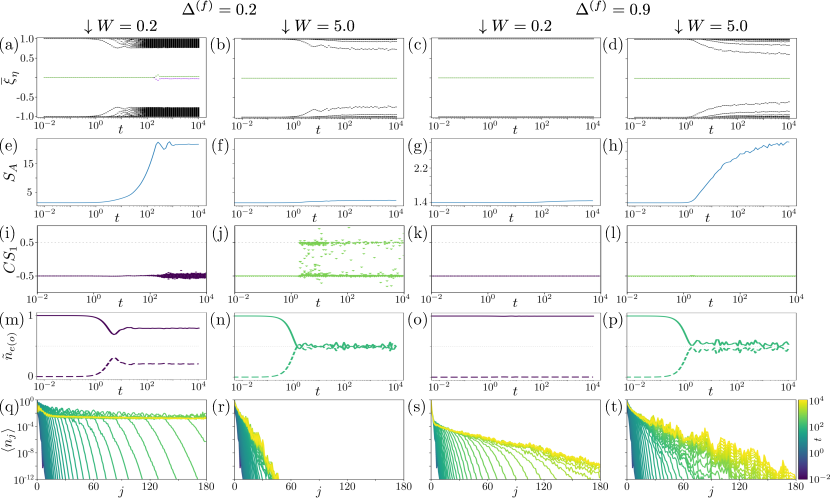
Figure S1: Quench on the system with OBC, finite $\Delta^{(f)}$ and two values of $W$. (a-d) Realisation-averaged ES (e-h) Realisation-averaged EE (i-l) All realisations of $CS_{1}$ calculated using $1\times 10^{4}$ $k$-points (m-p) Realisation-averaged Majorana distribution, $\tilde{n}_{e(o)}$, with even (odd) populations indicated by solid (dashed) curves (q-t) Realisation-averaged population profiles. Parameters are: (a,e,i,m,q) $(\Delta^{(f)},~{}W)=(0.2,~{}0.2)$, (b,f,j,n,r) $(\Delta^{(f)},~{}W)=(0.2,~{}5.0)$, (c,g,k,o,s) $(\Delta^{(f)},~{}W)=(0.9,~{}0.2)$ and (d,h,l,p,t) $(\Delta^{(f)},~{}W)=(0.9,~{}5.0)$, with all other parameters as in Fig. 1(a) of the main text.

IV Quenches with finite $\Delta^{(f)}$

Throughout the main body of this paper we have chosen, for simplicity, to focus primarily on quenches with $\Delta^{(f)}=0$. In the following we shall demonstrate that the results for this unique case are also applicable in the presence of finite pairing, but that we reach a different transport regime when the magnitude of $\Delta^{(f)}$ approaches the value of $J^{(f)}$.

When $\Delta^{(f)}=0.2$ we find that the ES and localisation profiles retain the features previously observed for $\Delta^{(f)}=0$. Figures S1 (q, r) show that the localization of the MZMs follows the same trend as in Figs. 3 (e,f) of the main text, with the edge mode continuing to extend across the chain for small disorder but becoming strongly localized when in the presence of large disorder. This once again results in a gapped ES for small $W$ (Fig. S1 (a)) and a gapless ES for large $W$ (Fig. S1 (b)). We note additionally, that the value of $\Delta^{(f)}$ plays a strong role in determining the entanglement gap between the ES zero modes and the bulk modes. As such, whilst the EE spectrum in Fig. S1 (e) qualitatively exhibits the same profile as for $\Delta^{(f)}=0$, it does not reach the same magnitude (see Fig. 3 (g)) since it is values in the ES that are closest to zero which contribute greatest to the EE.

On the other hand, when $\Delta^{(f)}=\Delta^{(i)}=0.9$ the ES remains gapless irrespective of the value of disorder (Figs. S1 (c-d)), indicating that correlations are inhibited from spreading throughout the chain. Likewise, the MZMs remain exponentially localized to the edges (Figs. S1 (s-t)), although the profile for higher disorder now extends further from the edge. While it seems counter-intuitive that for large disorder the localization profile seems less localized than for lower disorder, it can be understood simply by considering the tunneling pathways available between Majoranas. When the pairing approaches the value of the inter-site hopping, terms appearing as $J-|\Delta|$ in Eq. S1 will vanish. The post-quench Hamiltonian then reduces to a chain of $2N$ Majoranas with alternating hopping amplitudes $J+|\Delta|$ and $\mu_{j}$. Consequentially, increasing disorder (and therefore $\mu_{j}$) enhances transport between odd/even Majorana subspecies (as can be seen in Fig. S1 (p)) and thus results in further propagation from the edge. This also supports the spreading of correlations throughout the system, demonstrated by an increase in EE at long time when increasing disorder from $W=0.2$ (Fig. S1 (g)) to $W=5.0$ (Fig. S1 (h)).

Interestingly, the finite value of $\Delta^{(f)}$ has the additional effect of suppressing oscillations in $CS_{1}$, though greater values of $\Delta^{(f)}$ are required to overcome oscillations when in the presence of larger disorder (see Fig. S1(i-l)). This also reduces the density of the $k-$space grid required to resolve $CS_{1}$ as compared to Fig. 1(b,c) of the main text.

From the above, and by observing other intermediate values of $\Delta^{(f)}$, we find that the maximum $W$ for which ES gap openings are present decreases as $\Delta^{(f)}$ increases. Moreover, oscillations in $CS_{1}$ are suppressed for sequentially higher values of $W$ as $\Delta^{(f)}$ grows. Altogether, this suggests that in the intermediate regime, when $0<\Delta^{(f)}<\Delta^{(i)}$, there is a smooth crossover between the data presented in the main text and that shown for $\Delta^{(f)}=\Delta^{(i)}$ in the r.h.s of Fig. S1. Therefore, the presence of extended edge modes and an ES gap opening are not unique to the $\Delta^{(f)}=0$ boundary line, but rather extend to a large region in parameter space, tunable via the parameters of the system.

References

- Altland and Zirnbauer [1997] A. Altland and M. R. Zirnbauer, Phys. Rev. B 55, 1142 (1997).
- Kitaev [2009] A. Kitaev, AIP Conf. Proc. 1134, 22 (2009).
- Ryu et al. [2010] S. Ryu, A. P. Schnyder, A. Furusaki, and A. W. W. Ludwig, New J. Phys. 12, 065010 (2010).
- Chiu et al. [2016] C.-K. Chiu, J. C. Y. Teo, A. P. Schnyder, and S. Ryu, Rev. Mod. Phys. 88, 035005 (2016).
- McGinley and Cooper [2019] M. McGinley and N. R. Cooper, Phys. Rev. B 99, 075148 (2019).
- Chung et al. [2013] M.-C. Chung, Y.-H. Jhu, P. Chen, and C.-Y. Mou, J. Phys.: Condens. Matter 25, 285601 (2013).
- Hegde et al. [2015] S. Hegde, V. Shivamoggi, S. Vishveshwara, and D. Sen, New J. Phys. 17, 053036 (2015).
- Hegde and Vishveshwara [2016] S. S. Hegde and S. Vishveshwara, Phys. Rev. B 94, 115166 (2016).
- Chung et al. [2016] M.-C. Chung, Y.-H. Jhu, P. Chen, C.-Y. Mou, and X. Wan, Sci. Rep. 6, 29172 (2016).
- McGinley and Cooper [2018] M. McGinley and N. R. Cooper, Phys. Rev. Lett. 121, 090401 (2018).
- Gong and Ueda [2018] Z. Gong and M. Ueda, Phys. Rev. Lett. 121, 250601 (2018).
- Sedlmayr et al. [2018] N. Sedlmayr, P. Jaeger, M. Maiti, and J. Sirker, Phys. Rev. B 97, 064304 (2018).
- Pastori et al. [2020] L. Pastori, S. Barbarino, and J. C. Budich, Phys. Rev. Res. 2, 033259 (2020).
- Sayyad et al. [2021] S. Sayyad, J. Yu, A. G. Grushin, and L. M. Sieberer, Phys. Rev. Res. 3, 033022 (2021).
- Zhang et al. [2022] L. Zhang, W. Jia, and X.-J. Liu, Sci. Bull. 67, 1236 (2022).
- Fang et al. [2022] P. Fang, Y.-X. Wang, and F. Li, Phys. Rev. A 106, 022219 (2022).
- Wu et al. [2023] X. Wu, P. Fang, and F. Li, Phys. Rev. A 107, 052209 (2023).
- Song and Prodan [2014] J. Song and E. Prodan, Phys. Rev. B 89, 224203 (2014).
- Tao et al. [2020] Z. Tao, T. Yan, W. Liu, J. Niu, Y. Zhou, L. Zhang, H. Jia, W. Chen, S. Liu, Y. Chen, and D. Yu, Phys. Rev. B 101, 035109 (2020).
- Rančić [2022] M. J. Rančić, Scientific Reports 12, 19882 (2022).
- Dvir et al. [2023] T. Dvir, G. Wang, N. van Loo, C.-X. Liu, G. P. Mazur, A. Bordin, S. L. D. ten Haaf, J.-Y. Wang, D. van Driel, F. Zatelli, X. Li, F. K. Malinowski, S. Gazibegovic, G. Badawy, E. P. A. M. Bakkers, M. Wimmer, and L. P. Kouwenhoven, Nature 614, 445 (2023).
- Kitaev [2001] A. Y. Kitaev, Phys.-Usp. 44, 131 (2001).
- Vidal et al. [2003] G. Vidal, J. I. Latorre, E. Rico, and A. Kitaev, Phys. Rev. Lett. 90, 227902 (2003).
- Calabrese and Cardy [2004] P. Calabrese and J. Cardy, Journal of Statistical Mechanics: Theory and Experiment 2004, P06002 (2004).
- Eisert et al. [2010] J. Eisert, M. Cramer, and M. B. Plenio, Rev. Mod. Phys. 82, 277 (2010).
- Anderson [1958] P. W. Anderson, Phys. Rev. 109, 1492 (1958).
- Zak [1989] J. Zak, Phys. Rev. Lett. 62, 2747 (1989).
- Budich and Ardonne [2013] J. C. Budich and E. Ardonne, Phys. Rev. B 88, 075419 (2013).
- Rahul et al. [2019] S. Rahul, R. R. Kumar, Y. R. Kartik, A. Banerjee, and S. Sarkar, Phys. Scr. 94, 115803 (2019).
- Auckly [1994] D. R. Auckly, Math. Proc. Cambridge Philos. Soc. 115, 229–251 (1994).
- Chang [2018] P.-Y. Chang, Phys. Rev. B 97, 224304 (2018).
- Yang et al. [2018] C. Yang, L. Li, and S. Chen, Phys. Rev. B 97, 060304(R) (2018).
- Hsu et al. [2021] H.-C. Hsu, P.-M. Chiu, and P.-Y. Chang, Phys. Rev. Res. 3, 033242 (2021).
- [34] See Supplemental Material for more details.
- Sedlmayr [2019] N. Sedlmayr, Acta Phys. Pol. A 135, 1191 (2019).
- Fisher [1965] M. E. Fisher, The nature of critical points (University of Colorado Press, 1965).
- Fisher [1967] M. E. Fisher, Rep. Prog. Phys. 30, 615 (1967).
- Jalabert and Pastawski [2001] R. A. Jalabert and H. M. Pastawski, Phys. Rev. Lett. 86, 2490 (2001).
- Vajna and Dóra [2015] S. Vajna and B. Dóra, Phys. Rev. B 91, 155127 (2015).
- Budich and Heyl [2016] J. C. Budich and M. Heyl, Phys. Rev. B 93, 085416 (2016).
- Zhang and Song [2020] K. L. Zhang and Z. Song, Phys. Rev. B 101, 014303 (2020).
- Heyl [2018] M. Heyl, Rep. Prog. Phys. 81, 054001 (2018).
- Vanhala and Ojanen [2023] T. I. Vanhala and T. Ojanen, Phys. Rev. Res. 5, 033178 (2023).
- Sedlmayr and Bena [2015] N. Sedlmayr and C. Bena, Phys. Rev. B 92, 115115 (2015).
- Note [1] This is a direct consequence of the initial discrete symmetries: TRS makes real when is real; PHS maps any finite energy state into an orthogonal one, except for the Majoranas. The ChS is a composition of TRS and PHS. TRS is represented by the complex conjugation because of , so the corresponding PHS eigenvalues classify the MZMs.
- Li and Haldane [2008] H. Li and F. D. M. Haldane, Phys. Rev. Lett. 101, 010504 (2008).
- Legner and Neupert [2013] M. Legner and T. Neupert, Phys. Rev. B 88, 115114 (2013).
- Patrick et al. [2017] K. Patrick, T. Neupert, and J. K. Pachos, Phys. Rev. Lett. 118, 267002 (2017).
- Fidkowski [2010] L. Fidkowski, Phys. Rev. Lett. 104, 130502 (2010).
- Chandran et al. [2011] A. Chandran, M. Hermanns, N. Regnault, and B. A. Bernevig, Phys. Rev. B 84, 205136 (2011).
- Pollmann et al. [2010] F. Pollmann, A. M. Turner, E. Berg, and M. Oshikawa, Phys. Rev. B 81, 064439 (2010).
- Cho and Kim [2017] J. Cho and K. W. Kim, Sci. Rep. 7, 2745 (2017).
- Peschel [2003] I. Peschel, J. Phys. A: Math. Gen. 36, L205 (2003).
- Peschel and Eisler [2009] I. Peschel and V. Eisler, J. Phys. A Math. Theor. 42, 504003 (2009).
- Note [2] Since for sufficiently large systems the zero modes are approximately degenerate, we choose to take a linear superposition in the zero energy subspace, resulting in two zero modes appearing in the ES. See [34] for a more detailed explanation.
- Note [3] Whilst for an individual realization the left- and right-localized MZMs will, in general, have different profiles, on average we find that they qualitatively exhibit the same dynamics. As such, we choose to discuss solely the left-localized modes for brevity.
- Senthil [2015] T. Senthil, Annu. Rev. Condens. Matter Phys. 6, 299 (2015).
- Hastings [2007] M. B. Hastings, J. Stat. Mech. 2007, P08024 (2007).
- Brandão and Horodecki [2013] F. G. S. L. Brandão and M. Horodecki, Nat. Phys. 9, 721 (2013).
- Verresen et al. [2017] R. Verresen, R. Moessner, and F. Pollmann, Phys. Rev. B 96, 165124 (2017).
- Gurarie [2011] V. Gurarie, Phys. Rev. B 83, 085426 (2011).
- Manmana et al. [2012] S. R. Manmana, A. M. Essin, R. M. Noack, and V. Gurarie, Phys. Rev. B 86, 205119 (2012).
- Anderson [1967] P. W. Anderson, Phys. Rev. Lett. 18, 1049 (1967).
Supplemental Material: Extended edge modes and disorder preservation of a symmetry-protected topological phase out-of-equilibrium
In Section I we present the Hamiltonian and detail its symmetries in the Majorana representation. We show explicitly the one-particle correlation functions expressed in each basis. Section II summarizes the tools used to analyze the pseudospin dynamics and the topological state of the system. After introducing the concepts in periodic systems, we generalize them to the inhomogeneous case which is necessary due to disorder. In Section III we give further details about the Loschmidt echo. Finally, in Section IV, we provide and discuss the results of quenches with finite post-quench pairing amplitude.