Exact solution of Boltzmann equation in a longitudinal expanding system

Abstract

Analytical solutions to the microscopic Boltzmann equation are useful in testing the applicability and accuracy of macroscopic hydrodynamic theory. In this work, we present exact solutions of the relativistic Boltzmann equation, based on a new family of exact solutions of the relativistic ideal hydrodynamic equations [1]. To the best of our knowledge, this is the first exact solution that allows either symmetric or asymmetric longitudinal expansion with broken boost invariance.

Introduction. Hydrodynamics is a macroscopic, long-wavelength effective theory that describes the collective motions in many-body systems. The commonly used framework of relativistic hydrodynamic equations is derived from the microscopic Boltzmann equations by taking different approximations, such as relaxation time approximation [2], Chapman–Enskog expansion [3, 4], and moment expansion based methods by Isreal–Steward [5] and Denicol et al [6, 7, 8]. In these derivations, the systems are assumed to be close to local equilibrium, and the distribution function is the thermal equilibrium one plus small derivations expanded in different bases. The hydrodynamic theory only keeps lower order moments in the Knudsen expansion, leaving the higher order ones either truncated out or extrapolated under certain assumptions. Therefore, it is traditionally expected to be applicable in near-equilibrium systems with a small Knudsen number.

The success of applying hydrodynamic theory to describe the final state observables of collective motion in high energy nucleus-nucleus, proton-nucleus, and even proton-proton collisions (see e.g., [9, 10, 11, 12]) has drawn significant interests in discussions of relieving the assumptions for the applicability of hydrodynamics [13, 14, 15, 16, 17, 18, 19, 20, 21, 22, 23, 24, 25, 26, 27, 28, 29, 30, 31]. A crucial step is to compare the hydro results to those of the Boltzmann equation, which describes the evolution of the microscopic particle distribution.

Taking the general form in a curvilinear coordinates, the Boltzmann equation for on-shell distribution function reads, (see e.g.,  [32, 33, 34])

$$\begin{split}&\Big{(}p^{\mu}\partial_{\mu}+{\Gamma^{\rho}}_{\mu\nu}p^{\mu}p_{\rho}\frac{\partial}{\partial p_{\nu}}\Big{)}f(x^{\alpha},p_{\beta})=\mathcal{C}[f]\,,\\ &\mathcal{C}[f]=\frac{p_{\mu}u^{\mu}(x)}{\tau_{r}(x)}\Big{(}f(x^{\alpha},p_{\beta})-f_{eq}(x^{\alpha},p_{\beta})\Big{)}\,,\end{split}$$ (1)

where we have taken the relaxation time approximation(RTA) [2] for the collisions kernel. The Christoffel symbol is given by ${\Gamma^{\rho}}_{\mu\nu}=\frac{g^{\rho\gamma}}{2}\Big{(}\frac{\partial g_{\gamma\mu}}{\partial x^{\nu}}+\frac{\partial g_{\gamma\nu}}{\partial x^{\mu}}-\frac{\partial g_{\mu\nu}}{\partial x^{\gamma}}\Big{)}$, with $g^{\mu\nu}$ being the metric. Taking the conformal limit that $m=0$, the relaxation time reads $\tau_{r}(\hat{x})=5\bar{\eta}/\hat{T}(\hat{x})$, and $\bar{\eta}$ is the shear viscosity to entropy ratio [6, 7, 35, 36]. The local equilibrium distribution function is assumed to be of Boltzmann form, $f_{eq}=\exp(-\hat{p}_{\mu}\hat{u}^{\mu}/\hat{T})$. For the distribution functions in Eq. (1), all momentum arguments are covariant and coordinate arguments are contravariant. $\hat{T}(\hat{x})$ and $\hat{u}^{\mu}(\hat{x})$ are respectively the space-time dependent temperature and velocity. The space-time profiles of $\hat{T}$ and $\hat{u}^{\mu}$ are not arbitrary — they are constrained by continuity relations such as hydrodynamics.

In a given coordinate system, if one makes certain assumptions such that the Boltzmann equation can be expressed in a form without the derivatives with respect to the spatial coordinates and momenta, there exists a formal solution [37, 35, 36]. With explicit form which will be shown later in the main text, the formal solution depends only on the temporal coordinate and is homogeneous with respect to the spacial one. The non-trivial spatial expansion can be introduced if one takes a coordinate of a co-moving frame of a known solution to the hydrodynamic equations [38, 39, 40, 41]. A family of exact solutions for ideal fluids is found, recently, in [1], which is homogeneous in the transverse plane and allows expansion — either symmetric or asymmetric — in the longitudinal direction which breaks the boost invariance. In this work, we find the co-moving frame of the new solution and construct the formal solution accordingly. We then compute the hydrodynamics quantities and analyze how they relax to the hydro limit.

Co-moving frame of the longitudinal expanding flow. Taking the general form in a curvilinear coordinates, the hydrodynamic equation reads

$$\mathcal{D}_{\mu}T^{\mu\nu}\equiv\partial_{\mu}T^{\mu\nu}+\Gamma^{\mu}_{\ \rho\mu}T^{\rho\nu}+\Gamma^{\nu}_{\ \rho\mu}T^{\rho\mu}=0,$$ (2)

where $T^{\mu\nu}$ is the energy-momentum tensor, $\mathcal{D}_{\mu}$ is the covariant derivative. In Ref. [1], a family of exact solutions for longitudinally expanding ideal fluids was found,

$$\begin{split}\frac{T_{\mathrm{ideal}}}{T_{i}}=&\;\bigg{(}\frac{t_{0}}{\tau_{i}}+\frac{a\,\tau e^{\eta}}{\tau_{i}}\bigg{)}^{\frac{1-c_{s}^{2}}{4}\frac{1}{a^{2}}-\frac{1+c_{s}^{2}}{4}}\\ &\;\times\bigg{(}\frac{t_{0}}{\tau_{i}}+\frac{\tau e^{-\eta}}{a\,\tau_{i}}\bigg{)}^{\frac{1-c_{s}^{2}}{4}a^{2}-\frac{1+c_{s}^{2}}{4}}\,,\\ u^{\tau}=&\;\frac{1}{2}\Bigg{(}\sqrt{\frac{t_{0}e^{-\eta}+\tau\,a}{t_{0}e^{\eta}+\tau/a}}+\sqrt{\frac{t_{0}e^{\eta}+\tau/a}{t_{0}e^{-\eta}+\tau\,a}}\Bigg{)}\,,\\ u^{\eta}=&\frac{1}{2\tau}\Bigg{(}\sqrt{\frac{t_{0}e^{-\eta}+\tau\,a}{t_{0}e^{\eta}+\tau/a}}-\sqrt{\frac{t_{0}e^{\eta}+\tau/a}{t_{0}e^{-\eta}+\tau\,a}}\Bigg{)}.\end{split}$$ (3)

In the solution, $\tau$ and $\eta$ are the proper-time and rapidity in Milne coordinates, respectively. $c_{s}$ is the speed of sound, $a$ is a dimensionless parameter characterizing the asymmetry between forward and backward rapidity range, $T_{i}$ and $\tau_{i}$ are positive constants that respectively scale the temperature and time, and $t_{0}$ is an non-negative constant with units of time and it serves as a translation of the Minkowski time.

In this work, we introduce a new coordinate system which can be transformed from the Milne coordinates

$$\begin{split}\hat{x}^{0}=\;&\frac{2a}{1+a^{2}}\Big{(}(t_{0}+a\,\tau e^{\eta})^{\frac{1}{a}}({t}_{0}+\frac{\tau e^{-\eta}}{a})^{a}\Big{)}^{\frac{1+a^{2}}{4a}}\,,\\ \hat{x}^{1}=\;&\frac{1+a^{2}}{4a}\ln\Big{(}(t_{0}+a\,\tau e^{\eta})^{\frac{1}{a}}\big{/}({t}_{0}+\frac{\tau e^{-\eta}}{a})^{a}\Big{)}\,,\\ \hat{x}^{x}=\;&x,\qquad\qquad\hat{x}^{y}=y.\end{split}$$ (4)

The corresponding metric is

$$\hat{g}^{\mu\nu}=\mathrm{diag}\Big{[}e^{2\frac{1-a^{2}}{1+a^{2}}\hat{x}^{1}},-(\hat{x}^{0})^{-2}e^{2\frac{1-a^{2}}{1+a^{2}}\hat{x}^{1}},-1,-1\Big{]}\,,$$ (5)

and the non-vanishing components of the Christoffel symbol are

$$\begin{split}&\hat{\Gamma}^{0}_{\;\,11}=\hat{x}^{0}\,,\quad\hat{\Gamma}^{1}_{\;\,10}=\hat{\Gamma}^{1}_{\;\,01}=\frac{1}{\hat{x}^{0}}\,,\\ &\hat{\Gamma}^{0}_{\;\,01}=\hat{\Gamma}^{0}_{\;\,10}=\hat{\Gamma}^{1}_{\;\,11}=(\hat{x}^{0})^{2}\hat{\Gamma}^{1}_{\;\,00}=\frac{a^{2}-1}{a^{2}+1}\,.\end{split}$$ (6)

From now on, we take the “hat” ($\hat{\cdot}$) notation to denote quantities under the new coordinate system (4). Under the co-moving frame, the solution (3) becomes “static” that all spatial components vanish, and the space-time profile of the solution reads

$$\begin{split}&\hat{T}_{\mathrm{ideal}}=\sqrt{\hat{g}^{00}}\,T_{i}\,\Big{(}\frac{\tau_{i}}{\hat{x}^{0}}\Big{)}^{c_{s}^{2}}\,,\\ &\hat{u}^{0}=\sqrt{\hat{g}^{00}}\,,\quad\hat{u}^{1}=\hat{u}^{x}=\hat{u}^{y}=0\,.\end{split}$$ (7)

Therefore, (4) is the the co-moving frame of the asymmetric expanding flow (3).

Taking $t_{0}=0$ and $a=1$, Eq. (4) returns to the Milne coordinate and Eq. (7) returns to the Bjorken–Hwa solution [42, 43]. With general values for $t_{0}$ and $a$, one may still connect the new solution with the Bjorken–Hwa solution by re-scaling $\hat{u}^{\mu}$ and $\hat{T}$ by $(\hat{g}^{00})^{-1/2}$ and replacing $\hat{x}^{0}$ by $\tau$. $\hat{x}^{0}$ and $\hat{x}^{1}$, thus, are respectively referred to as the hat-proper-time and hat-rapidity in this paper.

The Boltzmann equation in the co-moving frame. Noting the simplicity of the solution (7) in the co-moving frame (4) and its similarity to the Bjorken–Hwa solution, we take the co-moving frame and solve the Boltzmann equations. Following the property of the hydro solution, we focus on the systems that are homogeneous in the transverse plane, and the Boltzmann equation (1) in the co-moving frame becomes

$$\Big{(}\hat{g}^{00}\hat{p}_{0}\frac{\partial}{\partial{{\hat{x}}^{0}}}+\hat{g}^{11}\hat{p}_{1}\frac{\partial}{\partial{{\hat{x}}^{1}}}+\frac{a^{2}-1}{a^{2}+1}(\hat{p}_{x}^{2}+\hat{p}_{y}^{2})\frac{\partial}{\partial{{\hat{p}}_{1}}}\Big{)}f(\hat{x}^{\alpha},\hat{p}_{\beta})$$

$$=-\frac{\hat{p}_{0}\hat{u}^{0}\hat{T}(\hat{x}^{0})}{5\bar{\eta}}\Big{(}f(x^{\alpha},\hat{p}_{\beta})-f_{eq}(x^{\alpha},\hat{p}_{\beta})\Big{)}.$$ (8)

Noting that the solution (3) requires a simple relation between the pressure and the energy density, $P=c_{s}^{2}\varepsilon$, which corresponds to the conformal limit in a kinetic theory, we therefore focus on massless particles in this work. The non-vanishing prefactor of the derivative with respect to ${\hat{p}}_{1}$ posts challenges in getting exact solution of the Boltzmann equation: the formal solution [37, 35, 36] can no longer be applied in such cases. Nevertheless, we find that the ${\hat{x}}^{1}$- and ${\hat{p}}_{1}$-derivatives can be canceled in several conditions where extra constraints are enforced. A solution is to let $a=1$, bringing our hydro solution to the Bjorken–Hwa one with a Minkowski-time translation [1]. This naturally leads to a corresponding relation between solution to the Boltzmann equation and  [41]. Apart from this, there are two solutions allowing an arbitrary $a$, which will be discussed in what follows.

Exact solution in 1+1 D. One way to eliminate the momentum derivatives in (8) is to focus on the special solutions that $f\propto\delta(\hat{p}_{x})\delta(\hat{p}_{y})$. This is equivalent to considering a coordinate system with only $\hat{x}^{0}$ and $\hat{x}^{1}$ and we therefore call it a 1+1 dimensional solution. Under such a constraint, the on-shell condition becomes $\hat{p}_{0}={|\hat{p}_{1}|}/{\hat{x}^{0}}$, and the speed of sound for massless free particle is $c_{s}=1$. The hydro solution reads $\hat{T}(\hat{x})=({T_{i}\tau_{i}}/{\hat{x}^{0}})e^{\frac{1-a^{2}}{1+a^{2}}\hat{x}^{1}}$ and $\hat{u}^{0}=e^{\frac{1-a^{2}}{1+a^{2}}\hat{x}^{1}}$. We find that both the equilibrium distribution, $f_{eq}(\hat{x}^{0})=e^{-\frac{\hat{x}^{0}\hat{p}_{0}}{T_{i}\tau_{i}}}$, and the equivalent relaxation time are independent of $\hat{x}^{1}$. This further allow us to assume that the solution to be independent of the hat-rapidity, and Eq. (8) becomes

$$\partial_{\hat{x}^{0}}f(\hat{x}^{0},\hat{p}_{1})=-\frac{T_{i}\,\tau_{i}}{5\bar{\eta}\,\hat{x}^{0}}\Big{(}f(\hat{x}^{0},\hat{p}_{1})-\exp(-\frac{\hat{x}^{0}\hat{p}_{0}}{T_{i}\tau_{i}})\Big{)}.$$ (9)

With arbitrary initial distribution function given at hat-proper-time $\hat{x}^{0}_{i}$, $f_{i}(\hat{x}^{0}_{i},\hat{p}_{1})$, we find the analytical solution to the Boltzmann equation (9) is

$$f(\hat{x}^{0},\hat{p}_{1})=\Big{(}f_{i}(\hat{x}^{0}_{i},\hat{p}_{1})-e^{-\frac{|\hat{p}_{1}|}{T_{i}\,\tau_{i}}}\Big{)}\Big{(}\frac{\hat{x}^{0}_{i}}{\hat{x}^{0}}\Big{)}^{\frac{T_{i}\,\tau_{i}}{5\bar{\eta}}}+e^{-\frac{|\hat{p}_{1}|}{T_{i}\,\tau_{i}}}\,.$$ (10)

The solution exhibits properties of a global equilibrium — if the initial distribution is the equilibrium one, Eq. (10) does not evolve with “time”($\hat{x}^{0}$) and always remain equilibrium; on the other hand, any deviation from the equilibrium distribution decreases in $\hat{x}^{0}$ with power $-\frac{T_{i}\tau_{i}}{5\bar{\eta}}$.

It shall be worth noting that while $f(\hat{x}^{0},\hat{p}_{1})$ does not explicitly depend on hat-rapidity, the corresponding energy-momentum stress tensor still non-trivially depends on $\hat{x}^{1}$ via the Jacobian of the momentum integral (i.e., $\sqrt{\hat{g}^{00}}$). In other words, the $\hat{x}^{1}$-dependence of hydrodynamic quantities can be factored out as scaling constants.

Exact solution in 3+1D. Compared to the aforementioned 1+1 D solution, the longitudinal distribution of relativistic heavy-ion collisions particle production is better described by solutions in the 3+1 dimensional coordinate [1], even if the transverse profile are assumed to be homogeneous. It is, thus, important to find solutions of the Boltzmann equation in 3+1 D coordinates for realistic studies.

We notice that

$$\hat{g}^{11}\hat{p}_{1}\frac{\partial}{\partial{{\hat{x}}^{1}}}\hat{p}_{0}=\; \frac{1-a^{2}}{1+a^{2}}\frac{\hat{p}_{1}}{(\hat{x}^{0})^{2}}\frac{\hat{p}_{x}^{2}+\hat{p}_{y}^{2}}{\hat{p}_{0}},$$ (11)

$$\frac{a^{2}-1}{a^{2}+1}(\hat{p}_{x}^{2}+\hat{p}_{y}^{2})\frac{\partial}{\partial{{\hat{p}}_{1}}}\hat{p}_{0}=\; -\frac{1-a^{2}}{1+a^{2}}\frac{\hat{p}_{1}}{(\hat{x}^{0})^{2}}\frac{\hat{p}_{x}^{2}+\hat{p}_{y}^{2}}{\hat{p}_{0}},$$ (12)

once the on-shell condition, $\hat{p}_{0}=\sqrt{(\frac{\hat{p}_{1}}{\hat{x}^{0}})^{2}+\hat{g}_{00}(\hat{p}_{x}^{2}+\hat{p}_{y}^{2})}$, is imposed. Therefore, we take the Ansatz that distribution function momentum dependence reduces to the dependence of energy, i.e., $f(x^{\alpha},\hat{p}_{\beta})=f(x^{\alpha},\hat{p}_{0})$, and the ${\hat{x}}^{1}$- and ${\hat{p}}_{1}$-derivatives in Eq. (8) cancel with each other,

$$\Big{(}\hat{g}^{11}\hat{p}_{1}\frac{\partial}{\partial{{\hat{x}}^{1}}}+\frac{a^{2}-1}{a^{2}+1}(\hat{p}_{x}^{2}+\hat{p}_{y}^{2})\frac{\partial}{\partial{{\hat{p}}_{1}}}\Big{)}f(\hat{x}^{\alpha},\hat{p}_{0})=0\,.$$ (13)

In 3+1 D, a conformal system has $c_{s}=1/\sqrt{3}$, and the solution reads $\hat{T}=T_{i}\big{(}\frac{\tau_{i}}{\hat{x}^{0}}\big{)}^{\frac{1}{3}}\sqrt{\hat{g}^{00}}$ and $\hat{u}^{0}=\sqrt{\hat{g}^{00}}$. The Boltzmann equation takes a simple form,

$$\partial_{\hat{x}^{0}}f(\hat{x}^{0},\hat{p}_{0})=-\frac{T_{i}}{5\bar{\eta}}\Big{(}\frac{\tau_{i}}{\hat{x}^{0}}\Big{)}^{\frac{1}{3}}\Big{(}f(\hat{x}^{0},\hat{p}_{0})-e^{-\frac{\hat{p}_{0}}{T_{i}}(\frac{\hat{x}^{0}}{\tau_{i}})^{\frac{1}{3}}}\Big{)},$$ (14)

and the formal solution [37, 35, 36] is applicable,

$$\begin{split}f(\hat{x}^{0},\hat{p}_{0})=\;&D(\hat{x}^{0},\hat{x}^{0}_{i})f_{0}(\hat{x}^{0}_{i},\hat{p}_{i,0})\\ +\;&\frac{1}{5\bar{\eta}}\int_{\hat{x}^{0}_{i}}^{\hat{x}^{0}}d{\hat{x}}^{\prime}D(\hat{x}^{0},{\hat{x}}^{\prime})\tilde{T}({\hat{x}}^{\prime})f_{eq}({\hat{x}}^{\prime},\hat{p}_{0}^{\prime})\,.\end{split}$$ (15)

Here, $f_{0}(\hat{x}^{0}_{i},\hat{p}_{i,0})$ is the initial distribution at hat-proper-time $\hat{x}^{0}_{i}$, $\tilde{T}(\hat{x}^{0})\equiv\hat{T}(\hat{x}^{0},\hat{x}^{1})/\sqrt{\hat{g}^{00}(\hat{x}^{1})}$, the energies $\hat{p}_{i,0}$, $\hat{p}_{0}$, and $\hat{p}_{0}^{\prime}$ respectively follow the on-shell condition with hat-proper-time being $\hat{x}^{0}_{i}$, $\hat{x}^{0}$, and $\hat{x}^{\prime}$. $D(\hat{x}^{0},\hat{x}^{0}_{i})\equiv\exp\Big{[}-\frac{1}{5\bar{\eta}}\int_{\hat{x}^{0}_{i}}^{\hat{x}^{0}}\tilde{T}({\hat{x}}^{\prime})d{\hat{x}}^{\prime}\Big{]}$, and we have defined $\tilde{T}\equiv{\hat{T}}/{\hat{u}^{0}}$ which only depends on hat-proper-time. There is no simple explicit form for the integral of the solution (15). Nevertheless, we may solve the integral numerically, construct the stress tensor out of the distribution function, extract the macroscopic hydrodynamic quantities, and analyze their “time” evolution.

In addition to the stress tensor, one may compute arbitrary higher order moments in the co-moving frame,

$$\hat{\mathcal{M}}^{\mu\nu\cdots\lambda}(\hat{x})\equiv\int(\hat{p}^{\mu}\hat{p}^{\nu}\cdots\hat{p}^{\lambda})f(\hat{x},\hat{p})d\hat{P}\,,$$ (16)

and then perform the transformation of tensor to obtain the corresponding moments in the either Milne or Minkowski coordinates,

$$\mathcal{M}^{\mu\nu\cdots\lambda}(x)=\bigg{(}\frac{\partial x^{\mu}}{\partial\hat{x}^{\mu^{\prime}}}\frac{\partial x^{\nu}}{\partial\hat{x}^{\nu^{\prime}}}\cdots\frac{\partial x^{\lambda}}{\partial\hat{x}^{\lambda^{\prime}}}\bigg{)}\hat{\mathcal{M}}^{\mu^{\prime}\nu^{\prime}\cdots\lambda^{\prime}}(\hat{x})\,.$$ (17)

The $\mathcal{M}^{\mu\nu\cdots\lambda}$’s are then useful in studying the emergency of hydro modes via the comparison with quantities in different frameworks of hydrodynamic equations.

Hydrodynamic quantities. Given the distribution function, the energy momentum tensor reads

$$\hat{T}^{\mu\nu}=\int d\hat{P}\,\hat{p}^{\mu}\hat{p}^{\nu}f(\hat{x},\hat{p}),$$ (18)

where $\int d\hat{P}\equiv\int\sqrt{-\hat{g}}\frac{d^{4}\hat{p}}{(2\pi)^{3}}\delta(\hat{p}^{0}(\hat{\bf p}))$. In the conformal limit, the bulk viscosity vanishes, and one can always decompose stress tensor as

$$\hat{T}^{\mu\nu}=\hat{\varepsilon}(\hat{x})\hat{u}^{\mu}\hat{u}^{\nu}+\Delta^{\mu\nu}\hat{\mathcal{P}}(\hat{x})+\hat{\pi}^{\mu\nu}(\hat{x})\,,$$ (19)

where $\hat{\varepsilon}(\hat{x})$ is the energy density, $\hat{\mathcal{P}}(\hat{x})$ the thermodynamic pressure, $\hat{\pi}^{\mu\nu}(\hat{x})$ the shear viscous stress tensor, and $\hat{\Delta}^{\mu\nu}\equiv\hat{g}^{\mu\nu}-\hat{u}^{\mu}\hat{u}^{\nu}$ the “space” projection operator. $\hat{\pi}^{\mu\nu}$ is symmetric, traceless ($\hat{g}_{\mu\nu}\hat{\pi}^{\mu\nu}=0$), and orthogonal to the fluid velocity ($\hat{u}_{\mu}\hat{\pi}^{\mu\nu}=\hat{u}_{\nu}\hat{\pi}^{\mu\nu}=0$). For massless particles in 3+1 D, the energy density, thermodynamic pressure, and entropy only depend on temperature

$$\hat{\varepsilon}=\frac{3\,\hat{T}^{4}}{2\pi^{2}}\,,\quad\hat{P}=\frac{\hat{T}^{4}}{2\pi^{2}}\,,\quad\hat{s}=\frac{\hat{\varepsilon}+\hat{P}}{\hat{T}}=\frac{2\,\hat{T}^{3}}{\pi^{2}}\,.$$ (20)

Placing $\int d\hat{P}\,\hat{p}^{\mu}\hat{p}^{\nu}$ on both side of Eq. (15), we obtain the integration form of the stress tensor,

$$\begin{split}\;&\hat{T}^{\mu\nu}(\hat{x})=D(\hat{x}^{0},\hat{x}^{0}_{i})\mathcal{H}^{\mu\nu}(\hat{x},\hat{x}^{0}_{i})\int\frac{p^{3}dp}{4\pi^{2}}f_{0}(\hat{x}^{0}_{i},\hat{p}_{i,0})\\ +\;&\frac{1}{5\bar{\eta}}\int_{\hat{x}^{0}_{i}}^{\hat{x}^{0}}d{\hat{x}}^{\prime}D(\hat{x}^{0},{\hat{x}}^{\prime})\tilde{T}({\hat{x}}^{\prime})\mathcal{H}^{\mu\nu}(\hat{x},\hat{x}^{\prime})\int\frac{p^{3}dp}{4\pi^{2}}f_{eq}(\hat{x}^{\prime},\hat{p}_{0}^{\prime}),\end{split}$$ (21)

with non-vanishing elements of tensor $\mathcal{H}^{\mu\nu}(\hat{x},\hat{y}^{0})$ given by

$$\begin{split}\mathcal{H}^{00}(\hat{x},\hat{y}^{0})\equiv\;&\frac{(\hat{g}^{00})^{3}}{4\pi}\frac{\hat{y}^{0}}{\hat{x}^{0}}\int\frac{\sin\theta d\theta d\varphi}{(\sin^{2}\theta+(\frac{\hat{y}^{0}}{\hat{x}^{0}})^{2}\cos^{2}\theta)^{-\frac{1}{2}}}\,,\\ \mathcal{H}^{11}(\hat{x},\hat{y}^{0})\equiv\;&\frac{(\hat{g}^{00})^{3}}{(\hat{x}^{0})^{2}4\pi}\Big{(}\frac{\hat{y}^{0}}{\hat{x}^{0}}\Big{)}^{3}\int\frac{\cos^{2}\theta\sin\theta d\theta d\varphi}{(\sin^{2}\theta+(\frac{\hat{y}^{0}}{\hat{x}^{0}})^{2}\cos^{2}\theta)^{\frac{1}{2}}}\,,\\ \mathcal{H}^{xx}(\hat{x},\hat{y}^{0})\equiv\;&\frac{(\hat{g}^{00})^{2}}{4\pi}\frac{\hat{y}^{0}}{\hat{x}^{0}}\int\frac{\sin^{2}\theta\cos^{2}\phi\sin\theta d\theta d\varphi}{(\sin^{2}\theta+(\frac{\hat{y}^{0}}{\hat{x}^{0}})^{2}\cos^{2}\theta)^{\frac{1}{2}}}\,,\end{split}$$ (22)

and $\mathcal{H}^{yy}(\hat{x},\hat{y}^{0})=\mathcal{H}^{xx}(\hat{x},\hat{y}^{0})$. Noting that $\hat{T}^{\mu\nu}$ is always diagonal, the fluid is still “at rest” in the co-moving frame, i.e., $\hat{u}^{\mu}$ in (7) remains the correct velocity decomposition of (21). For a conformal system that is homogeneous in the transverse plane, the stress tensor is traceless ($\hat{g}_{\mu\nu}\hat{T}^{\mu\nu}=0$) and symmetric when exchanging the transverse variables ($\hat{T}^{xx}=\hat{T}^{yy}$). There remains two independent components in the stress tensor — the effective temperature determined by $\hat{T}^{00}=\frac{3\,\hat{T}_{\mathrm{eff}}^{4}}{2\pi^{2}}\hat{u}^{0}\hat{u}^{0}$, and the shear viscous tensor $\hat{\pi}^{xx}\equiv\hat{T}^{xx}-\frac{\hat{T}^{00}}{3\hat{g}^{00}}$.

One can find that $\int\frac{p^{3}dp}{6}f_{eq}(\hat{x}^{\prime},\hat{p}_{i}^{\prime})=\frac{\hat{T}_{\mathrm{ideal}}^{4}(\hat{x}^{\prime},\hat{x}^{1})}{(\hat{g}^{00})^{2}}$ with temperature given in Eq. (7). We further denote that $\hat{T}_{0}(\hat{x}_{i}^{0},\hat{x}^{1})\equiv\sqrt{\hat{g}^{00}}\big{(}\int\frac{p^{3}dp}{6}f_{0}(\hat{x}^{0}_{i},\hat{p}_{i,0})\big{)}^{\frac{1}{4}}$, and the effective temperature and shear viscous stress tensor read

$$\begin{split}\hat{T}_{\mathrm{eff}}^{4}=\;&D(\hat{x}^{0},\hat{x}^{0}_{i})\tilde{\mathcal{H}}_{0}(\hat{x}^{0},\hat{x}_{i})\hat{T}^{4}_{0}(\hat{x}_{i}^{0},\hat{x}^{1})\\ +\;&\frac{1}{5\bar{\eta}}\int_{\hat{x}^{0}_{i}}^{\hat{x}^{0}}d{\hat{x}}^{\prime}D(\hat{x}^{0},{\hat{x}}^{\prime})\tilde{T}({\hat{x}}^{\prime})\tilde{\mathcal{H}}(\hat{x}^{0},\hat{x}^{\prime})\hat{T}_{\mathrm{ideal}}^{4}(\hat{x}^{\prime},\hat{x}^{1})\,,\\ \hat{\pi}^{xx}=\;&D(\hat{x}^{0},\hat{x}^{0}_{i})\tilde{\mathcal{H}}_{x}(\hat{x}^{0},\hat{x}_{i})\hat{T}^{4}_{0}(\hat{x}_{i}^{0},\hat{x}^{1})\\ +\;&\frac{1}{5\bar{\eta}}\int_{\hat{x}^{0}_{i}}^{\hat{x}^{0}}d{\hat{x}}^{\prime}D(\hat{x}^{0},{\hat{x}}^{\prime})\tilde{T}({\hat{x}}^{\prime})\tilde{\mathcal{H}}_{x}(\hat{x}^{0},\hat{x}^{\prime})\hat{T}_{\mathrm{ideal}}^{4}(\hat{x}^{\prime},\hat{x}^{1})\,,\end{split}$$ (23)

where $\tilde{\mathcal{H}}_{0}\equiv\frac{\mathcal{H}^{00}}{(\hat{g}^{00})^{3}}$ and $\tilde{\mathcal{H}}_{x}\equiv\frac{3}{2\pi^{2}}(\frac{\mathcal{H}^{xx}}{(\hat{g}^{00})^{2}}-\frac{\mathcal{H}^{00}}{3(\hat{g}^{00})^{3}})$ independent of $\hat{x}^{1}$. It is clear that the $\hat{x}^{1}$ dependence of both $\hat{T}_{0}(\hat{x}_{i},\hat{x}^{1})$ and $\hat{T}_{\mathrm{ideal}}(\hat{x}^{\prime},\hat{x}^{1})$ can be factored out as $\sqrt{\hat{g}^{00}}$, which makes $\hat{T}_{\mathrm{eff}}\propto\sqrt{\hat{g}^{00}}$ and $\hat{\pi}^{xx}\propto(\hat{g}^{00})^{2}$. We therefore look into scaled temperature $\hat{T}_{\mathrm{eff}}/\hat{T}_{\mathrm{ideal}}$ and scaled shear viscous stress tensor $\hat{\pi}^{xx}/(\hat{s}_{\mathrm{ideal}}\frac{\hat{u}^{0}}{\hat{x}^{0}})$, which are dimensionless and independent of the hat-rapidity, whose ”evolution” with hat-proper-time are shown in Fig. 1 for various $\bar{\eta}$. We note that the initial condition of $\hat{T}_{\mathrm{eff}}$ and $\hat{\pi}^{xx}$ depends only on $\hat{T}_{0}$, rather than the specific form of distribution function. The influence of the latter can be observed in higher order moments, e.g., $\int(\hat{p}_{0})^{n\geq 3}\,f\,d\hat{P}$. Matching condition of the energy density requires $\hat{T}_{0}(\hat{x}^{0}_{i},\hat{x}^{1})=\hat{T}_{\mathrm{ideal}}(\hat{x}^{0}=\hat{x}^{0}_{i},\hat{x}^{1})$. In making the plot, we have taken $\tau_{i}=\hat{x}^{0}_{i}$ and $T_{i}=1/\hat{x}^{0}_{i}$.

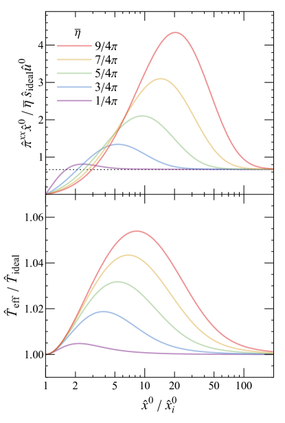
Figure 1: Scaled shear viscous stress tensor (upper) and scaled temperature (lower) as a function of $\hat{x}^{0}/{\hat{x}}_{i}^{0}$ obtained by different scaled shear viscosity to entropy ratios ($\bar{\eta}$). Black dashed curve in the upper panels indicate the Navier–Stokes limit $2/3$, whereas solid curves are respectively for $\bar{\eta}=1/4\pi$(purple), $3/4\pi$(blue), $5/4\pi$(green), $7/4\pi$(yellow), and $9/4\pi$(red).

For long hat-proper-time limit, perturbative analysis of (23) shows that

$$\frac{\hat{T}_{\mathrm{eff}}}{\hat{T}_{\mathrm{ideal}}}=\, 1+\frac{20\,\bar{\eta}^{2}}{9\,T_{i}^{2}\tau_{i}^{2}}\Big{(}\frac{\tau_{i}}{\hat{x}^{0}}\Big{)}^{\frac{4}{3}}+\mathcal{O}\big{(}(\hat{x}^{0})^{-2}\big{)}\,,$$ (24)

$$\frac{\hat{\pi}^{xx}\hat{x}^{0}}{\hat{s}_{\mathrm{ideal}}\hat{u}^{0}}=\, \frac{2\bar{\eta}}{3}+\frac{40\,\bar{\eta}^{2}}{63\,T_{i}\,\tau_{i}}\Big{(}\frac{\tau_{i}}{\hat{x}^{0}}\Big{)}^{\frac{2}{3}}+\mathcal{O}\big{(}(\hat{x}^{0})^{-\frac{4}{3}}\big{)}\,.$$ (25)

Starting from a initial condition which matches the ideal temperature, the scaled temperature first deviates from unity driven by the viscous effect, then it approaches the ideal limit at large enough $\hat{x}^{0}$. The scaled shear-viscous stress tensor starts from zero and grows to a large value, and then it decreases and approaches the Navier–Stokes limit. In both quantities, the leading order corrections are proportional to $\bar{\eta}^{2}$. Comparing the power in $\frac{\tau_{i}}{\hat{x}^{0}}$ we observe that correction of the scaled temperature decays faster than the scaled shear-viscous stress tensor, which is exhibited in Fig. 1.

Summary. In this work, we derive new analytical solutions to the Boltzmann equation, which take the relaxation time approximation for the collisions kernel, associated with a newly discovered exact solution of ideal hydrodynamics [1]. The solution assumes homogeneity in the transverse plane, and allows non-trivial rapidity dependence. This is the first analytical solution of the Boltzmann equation that allows asymmetric rapidity dependence, to the best of our knowledge. With the distribution function, we further construct the stress tensor and compute the effective temperature and shear viscous stress tensor. We observe that both the temperature and the shear viscous stress tensor relax to the limit of hydrodynamics. Our solution is useful in testing the applicability and accuracy of different approximations in the derivation of hydrodynamic equations.

Acknowledgement. The authors thank Dr. Lipei Du for helpful discussion. This work is supported by Tsinghua University under grant Nos. 53330500923 and 100005024.