Multi-Objective Transmission Expansion: An Offshore Wind Power Integration Case Study

Abstract

We describe a multi-objective, multistage generation, storage and transmission expansion planning (GS&TEP) model for the electric power sector, emphasizing coordinated offshore and onshore grid planning. Unlike traditional capacity expansion models that focus exclusively on investment and operational costs, our model explicitly accounts for negative externalities such as the social cost of greenhouse gas emissions and local damages from reduced air quality. We use an 8-zone representation of the ISO-NE system to study the sensitivity of grid expansion decisions with the primary focus on optimal capacity expansion decisions due to large-scale offshore wind power integration. Our model allows investment decisions to be made in multiple stages and accounts for short-term uncertainty during operations through scenarios. Our results indicate that considering externalities leads to greater upfront investment in cleaner generation and storage, which are largely offset by lower expected operational costs.

Nomenclature

Indices and Sets

• Years over the planning horizon.

• Representative days or scenarios.

• Hours on a representative day.

• Nodes or zones.

• Onshore/Offshore nodes.

• Generators.

• Dispatchable/Intermittent (non-dispatchable) generators.

• New/Existing generators.

• Generation technology types.

• Transmission lines.

• AC/DC transmission lines.

• New/Existing transmission lines.

• Onshore/Offshore transmission lines.

• Indices of sending/receiving nodes line $l$

• Line types.

• Flexible demand block.

• Externalities.

• Region for policy constraints.

Parameters

• Weighting parameter of discounted environmental externality costs

• Useful life of asset $(\cdot)$ in years.

• Discount rate.

• Cost per unit capacity of a generation technology type $k$.

• Cost per unit capacity-length of capacity of a transmission line of type $c$.

• Cost per unit power capacity of energy storage.

• Cost per unit energy capacity of battery storage.

• Annualized cost per unit capacity of a transmission line.

• Number of days in a year.

• Weight of representative days.

• Renewable Portfolio Standard in region $j$

• Policy mandate non-compliance penalty.

• Under-generation penalty.

• Over-generation penalty.

• Fixed annual operational cost per unit capacity of generator $i$.

• Variable operations cost of generator $i$.

• Willingness to pay for demand block $b$.

• Damage costs caused by externality $x$ per unit energy production by generator $i$.

• Minimum/Maximum power limits of generator $i$.

• Ramp rate of generator $i$.

• Temporal resolution of model.

• Duration (fraction of $\Delta h$) within which reserves should be supplied.

• Mapping of generator $i$, of type $k$, to node $s$.

• Mapping generator $i$ to node $s$.

• Mapping line $l$ to node $s$.

• Mapping line $l$ to type $c$.

• Mapping region $j$ to node $s$.

• Mapping offshore node $s$ to online year $y$.

• Forecasted load in year $y$, at node $s$, on representative day $e$, during hour $h$.

• Charging/Discharging efficiency of energy storage resources.

• Allowable depth of discharge of energy storage resources.

• Annual degradation factor of energy storage.

• Energy storage duration.

• Flow limit (capacity) of transmission line $l$ of type $c$.

• Susceptance of line $l$.

• Large positive number.

• Operating reserve requirement in year $y$, at node $s$, on representative day $e$, during hour $h$.

Binary variables

• Investment (or construction start) of line $l$, of type $c$ in year $y$.

• Availability of line $l$, of type $c$ in year $y$.

Continuous variables

• Discounted annual operational cost of asset ${(\cdot)}$ in year $y$.

• Discounted annual investment cost of asset ${(\cdot)}$ in year $y$.

• Discounted annual damage costs caused by externalities in year $y$.

• New generation capacity in year $y$ at $s$ of type $k$.

• Total generation of generator $i$ in year $y$, on representative day $e$, during hour $h$.

• Reserve provided by generator $i$ in year $y$, on representative day $e$, during hour $h$.

• Reserve provided by energy storage in year $y$, at node $s$, on representative day $e$, during hour $h$.

• Renewable energy curtailment in year $y$, at node $s$, on representative day $e$, during hour $h$.

• Unserved load in year $y$, at node $s$, on representative day $e$, during hour $h$.

• Flexible demand in year $y$, at node $s$, on representative day $e$, during hour $h$ (free variable).

• Policy target noncompliance in year $y$ in region $j$.

• Power flow through line $l$ in year $y$, on representative day $e$, during hour $h$.

• Voltage angle at node $s$ in year $y$, on representative day $e$, during hour $h$ (free variable).

I Introduction

Streamlining transmission expansion is required for decarbonization of U.S. electric grid [1, 2, 3]. This challenge is pertinent to increasing renewable penetration, the need to integrate offshore wind resources, and the expected load growth due to electrification of heating and transportation. Given that transmission investments last for decades, investing at the right place and time to ensure a cost-effective clean energy transition, while not sacrificing reliability, requires a planning framework that can take into account not only the cost and technology drivers but also such policy drivers as greenhouse gases, air pollution, and resilience to extreme weather events. At the same time, interregional transmission lines cross state lines, the cost of these lines and the debates if the resource preference of one region requires additional transmission upgrades in another region is a significant barrier to transmission development [4]. In the US, transmission planners seek to align centralized transmission network planning decisions with decentralized generation investments [5]. Furthermore, despite Federal Energy Regulatory Commission (FERC) Order 1000, which highlights the importance of regional and inter-regional planning, the majority of transmission planning processes in the U.S. are driven by local reliability needs and separated from generation planning [6].

The main focus of current transmission planning is to minimize “economic” costs for solving a local reliability need. Even if planners look at regional needs, most U.S. transmission planners rely on generation, storage and transmission expansion planning (GS&TEP) models, which include investment and operation cost estimates and often ignore any costs or benefits related to externalities such as greenhouse gas emissions and local air pollution from power generation that impose costs on society (including future generations). Similarly, there are societal benefits to a more reliable and resilient electric power system, particularly with an increasing frequency of climate-induced extreme weather events.

To overcome deficiencies of existing planning processes, FERC proposed to require transmission providers to conduct long-term regional transmission planning on a sufficiently forward-looking basis to meet the needs driven by changes in the resource mix and demand [7]. FERC lists externalities to include in the analysis, and asks transmission providers to develop selection criteria “to maximize benefits to consumers over time without over-building transmission facilities.” Similarly, National Grid UK has begun considering objectives other than just investment and operational costs when evaluating integration of offshore wind farms [8]. Another policy-relevant question for transmission planning is whether to minimize economic costs, or conversely, if active demand side participation is included, maximize economic welfare. Despite policy relevance, there is limited guidance in the economic or engineering literature on how to incorporate these factors or even whether these factors make a difference in the optimal investment topology, timing, or costs.

This paper uses a multi-objective modeling framework to answer these questions. We assume the perspective of the social planner performing joint centralized transmission and decentralized generation expansion planning, including offshore wind. Distinct from traditional approaches, we explicitly account for such externalities as greenhouse gas emissions, local air pollution and public health damage using multi-objective optimization in our GS&TEP models. Our results show that incorporating the externalities, along with the consideration of extreme weather events, results in markedly different outcomes. The proposed multi-objective transmission planning framework equips electric power regulators with a tool that can help overcome balancing multiple policy objectives and address externalities. Furthermore, our results show that considering these additional factors do not lead to significant changes in necessary onshore line investments, which may help alleviate tensions in the current policy debates.

I-A Literature Review

Various studies underscore diverse challenges and benefits of offshore wind power integration. For instance, Pfeifenberger et al. [6] underline the advantages of offshore mesh networks. Similarly, Musial et al. [9] stress the importance of inter-regional coordination for offshore transmission planning to achieve cost-effective and low-impact solutions. There also have been modeling studies, [10, 11, 12, 13], examining transmission options for the integration of offshore wind power, comparing AC and DC transmission options and cable routing. However, these studies do not capture non-economic benefits of large-scale offshore wind power integration that can be attained if co-designed with the onshore power system.

A rich literature exists on bottom-up, engineering-economic planning models and tools for the electric power sector, which consider both investment in and operation of generation, storage, and transmission assets, and utilization of electric power, while capturing their economic and environmental impacts. Muñoz et al. [14] describe an adaptive transmission and generation planning accounting for regulatory and market uncertainties. Qiu et al. [15] develop a co-planning framework for transmission and energy storage, where investment decisions are made in multiple stages and operational uncertainty is captured through representative scenarios.

Regardless of the objective, planning models strive to optimize investment and operational costs over a given planning horizon, while ignoring non-economic factors (e.g., emissions costs, air quality damages, resilience). With the rise in cost competitiveness and locational advantages of offshore wind power resources, this paper argues that these non-economic factors must be incorporated within transmission expansion planning to capture the full societal value of these resources and inform decision makers on trade-offs between economic and non-economic factors.

II Model

Fig. 1 illustrates the representation of multi-stage investments and operations in our model. Investments are allowed at the beginning of each epoch and system operations are modeled within each epoch. We account for operational uncertainty via a set of scenarios, consisting of representative (normal) and synthetic extreme days. Unless otherwise noted in the nomenclature as free variables, all decision variables in our model are constrained to be non-negative.

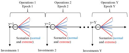
Figure 1: Stages for expansion decisions and operational scenario trees.

II-A Objective Functions

We enhance the GS&TEP model formulation of [15] by explicitly incorporating the societal cost of environmental externalities into the objective function in Eq. (1). Setting $\omega^{EC}=0$ reduces the objective function to the traditional planning paradigm, accounting only for economic costs, such as in [15].

$$\min z=\sum_{y\in\mathcal{Y}}OC_{y}+IC_{y}^{g}+IC_{y}^{l}+IC_{y}^{s}+\omega^{EC}\,EC_{y}$$ (1)

where generation($IC_{y}^{g}$), transmission line ($IC_{y}^{l}$), energy storage ($IC_{y}^{s}$) investment costs are scenario-independent, while variables related to system operations, e.g., costs from externalities ($EC_{y}$) and operations ($OC_{y}$), are scenario-dependent.

We adjust the annualized investment costs of technology to account for the varying lifespans of the technologies to be invested in by using the capital recovery factor (CRF) and the annual discount rate ($\gamma$). This allows consistent comparison between annualized investment costs across technologies.

$$\operatorname{CRF}^{(\cdot)}\mathrm{=\frac{r(1+\mathrm{r})^{{N}^{(\cdot)}}}{(1+\mathrm{r})^{{N}^{(\cdot)}}-1}}$$ (2)

$$\gamma_{n}^{(\cdot)}=\frac{\mathbf{1}_{n}^{(.)}}{(1+\mathrm{r})^{n-1}}$$ (3)

where, $\mathbf{1}_{n}^{(.)}$ is an indicator function, as defined in Eq. (4), denoting the availability of asset $(\cdot)$.

$$\mathbf{1}_{n}^{(.)}=\begin{cases}1&n\in\{1,\cdots,\mathrm{N}^{{(.)}}\}\\ 0&n\notin\{1,\cdots,\mathrm{N}^{(.)}\}\end{cases}$$ (4)

II-A1 Investment Cost

Eqs. (5)–(7) compute the generation, transmission, and storage discounted annual investment costs.

$$IC^{g}_{y} =\operatorname{CRF}^{g}\sum_{n=1}^{y}\gamma_{y-n+1}^{g}\sum_{k\in\mathcal{K}}\sum_{s\in\mathcal{S}}\mathrm{GC}_{k}\,{P}^{g}_{n,s,k}\quad\forall\,y$$ (5)

$$IC^{l}_{y} =\operatorname{CRF}^{l}\sum_{n=1}^{y}\gamma_{y-n+1}^{l}\sum_{l\in\mathcal{L}}\mathrm{LC}_{c}\,I^{l}_{l,c,n}\quad\forall\,y$$ (6)

$$IC_{y}^{s} =\operatorname{CRF}^{s}\sum_{n=1}^{y}\gamma_{y-n+1}^{l}\sum_{s\in\mathcal{S}}\left(\mathrm{SC}^{p}\,P_{s,n}^{s}+\mathrm{SC}^{e}\,E^{s}_{s,n}\right)\quad\forall\,y.$$ (7)

II-A2 Operation Cost

Eq. (8) calculates the discounted annual operating cost for each year in the future. It includes the cost of operation of existing and new resources, payment to demand response, renewable energy curtailment cost, unserved load penalty, and penalty for non-compliance with policy target.

$$OC_{y}=\frac{1}{(1+\mathrm{r})^{y-1}}\Biggl{\{}\mathrm{PEN}^{\times}\rho^{\times}_{y,j}+\sum_{i\in\mathcal{G}}\mathrm{FC}^{g}_{i}\,\overline{\mathrm{P}}_{i}^{g}+$$ (8)

$$\sum_{e\in\mathcal{E}}\tau\omega_{e}\Biggl{(}\sum_{i\in\mathcal{G}}\sum_{h\in\mathcal{H}}\mathrm{VC}^{g}_{i}\,p^{g}_{y,i,e,h}+\sum_{s\in\mathcal{S}}\sum_{h\in\mathcal{H}}OC^{p}_{y,s,e,h}$$

$$+\sum_{s\in\mathcal{S}}\sum_{h\in\mathcal{H}}OC^{d}_{y,s,e,h}\Biggr{)}\Biggr{\}}\quad\forall\,y.$$

In Eq. (8), the discounted penalty term ($OC^{p}_{y,s,e,h}$), for both over-supply or under-supply penalties, is given by:

$$\mathrm{PEN}^{+}\sum_{s\in\mathcal{S}}\sum_{h\in\mathcal{H}}\psi^{+}_{y,s,e,h}+\mathrm{PEN}^{-}\sum_{s\in\mathcal{S}}\sum_{h\in\mathcal{H}}\psi^{-}_{y,s,e,h}\quad\forall\,y,s,e,h$$ (9)

And, the demand (flexibility) cost ($OC^{d}_{y,s,e,h}$), where various demand blocks ($b$) are valued at different levels of willingness to pay for energy ($\mathrm{WP}_{b}$), is:

$$\sum_{b\in\mathcal{B}^{d}}\mathrm{WP}_{b}\,\left|\Delta{d_{y,s,e,h,b}}\right|\quad\forall\,y,s,e,h.$$ (10)

II-A3 Cost of Externalities

Given the costs of externalities per unit of energy production, the total cost of externalities in year $y$ is:

$$EC_{y} =\frac{1}{(1+\mathrm{r})^{y-1}}\sum_{e\in\mathcal{E}}\sum_{x\in\mathcal{X}}\tau\,\omega_{e}\sum_{i\in\mathcal{I}}\sum_{h\in\mathcal{H}}\mathrm{CE}_{i,x}\,p^{g}_{y,i,e,h}\quad\forall\,y.$$ (11)

II-B Operational Constraints

II-B1 Generator Limits

Eqs. (12)–(15) implement the constraints on capacity and ramping limits on generation and reserve provision. Eq. (16) makes new generation capacity available.

$$\underline{\mathrm{P}}^{g}_{i}\leq p^{g}_{y,i,e,h}\leq\overline{\mathrm{P}}^{g}_{i}\quad\forall\,y,i\in\mathcal{G^{D}}\cap\mathcal{G^{E}},e,h$$ (12)

$$p^{g}_{y,i,e,h}+r^{g}_{y,i,e,h}-p^{g}_{y,i,e,h-1}\leq\mathrm{RR}_{i}\quad\forall\,y,i\in\mathcal{G^{D}},e,h$$ (13)

$$-\mathrm{RR}_{i}\leq p^{g}_{y,i,e,h}-p^{g}_{y,i,e,h-1}-r^{g}_{y,i,e,h-1}\,\forall\,y,i\in\mathcal{G^{D}},e,h$$ (14)

$$r^{g}_{y,i,e,h}\leq\mathrm{RR}_{i}\,\mathrm{\delta h}\quad\forall\,y,i\in\mathcal{G^{D}},e,h$$ (15)

$${p}^{g}_{y,s,e,h}\,\mathrm{M}_{i,s,k}\leq\sum_{n=1}^{y}\mathbf{1}_{y-n+1}^{g}\,{P}^{g}_{n,s,k}\quad\forall\,y,s,e,h,k,i\in\mathcal{G^{N}}\cap\mathcal{G^{D}}$$ (16)

II-B2 Demand Flexibility

Eq. (17) bounds the demand flexibility as a fraction of the total demand. Eq. (18) ensures that loads can be shifted within a day.

$$\left|\sum_{b\in\mathcal{B^{D}}}\Delta{d_{y,s,e,h,b}}\right|\leq\phi\,\mathrm{D}_{y,s,e,h}\quad\forall\,y,s,e,h$$ (17)

$$\sum_{h\in\mathcal{H}}\sum_{b\in\mathcal{B^{D}}}\Delta{d_{y,s,e,h,b}}=0\quad\forall\,y,s,e$$ (18)

II-B3 Power Balance

Eqs. (II-B3)–(21) enforces the nodal power balance.

$$\sum_{i\in\mathcal{G}}p^{g}_{y,i,e,h}\,\mathrm{M}_{i,s}^{g}-\sum_{l\in\mathcal{L}}f_{y,l,e,h}\,\mathrm{M}_{l,s}^{l}$$

$$=\mathrm{D}_{y,s,e,h}+\Delta d_{y,s,e,h}+\psi^{+}_{y,s,e,h}-\psi^{-}_{y,s,e,h}$$

$$\quad+\frac{p^{s,ch}_{y,s,e,h}}{\eta^{s,ch}}-p^{s,dis}_{y,s,e,h}\eta^{s,dis}\quad\forall\,y,s,e,h$$ (19)

$$\psi^{-}_{y,s,e,h}\leq\mathrm{D}_{y,s,e,h}+\Delta d_{y,s,e,h}\quad\forall\,y,s,e,h$$ (20)

$$\psi^{+}_{y,s,e,h}\leq\sum_{i\in\mathcal{G^{I}}}p^{g}_{y,i,e,h}\,\mathrm{M}_{i,s}^{g}\quad\forall\,y,s,e,h.$$ (21)

II-B4 Reserve Requirement

Eq. (22) imposes reserve requirements for system operations.

$$\sum_{i\in\mathcal{G^{D}}}r^{g}_{y,i,e,h}+\sum_{s\in\mathcal{S}}r^{s}_{y,s,e,h}\geq\mathcal{R}^{\star}_{y,s,e,h}\quad\forall\,y,s,e,h.$$ (22)

II-B5 Energy Storage

While our energy storage model is broadly applicable to other types of energy storage, we have tailored it for grid-scale battery storage. In line with [15, 16], the battery energy storage system (BESS) planning and operation include tracking the state of charge (SoC) as per Eq. (II-B5), enforcing capacity limits as in Eqs. (26)–(29), and evaluating available energy and power capacities over time, as outlined in Eqs. (30) and (31), considering a constant annual degradation factor ($\kappa^{s}$). However, using a constant annual degradation factor may be an oversimplification of such operational factors as cycling, temperature, SoC, and depth of discharge (DoD).

$$SoC^{s}_{y,s,e,h}=SoC^{s}_{y,s,e,h-1}+p^{s,ch}_{y,s,e,h}\Delta h$$

$$-p^{s,dis}_{y,s,e,h}\Delta h\quad\forall\,y,s,e,h$$ (23)

$$\underline{E}^{s}_{s,y}=\mathrm{DoD}^{s}\,\overline{E}^{s}_{s,y}$$ (24)

$$SoC^{s}_{y,s,e,\min(\mathcal{H})},\,SoC^{s}_{y,s,e,\max(\mathcal{H})}=\mathrm{SoC}^{s,0}$$ (25)

$$p^{s,ch}_{y,s,e,h},p^{s,dis}_{y,s,e,h}\leq\overline{P}^{s}_{s,y}\quad\forall\,y,s,e,h$$ (26)

$$r^{s}_{y,s,e,h}+p^{s,dis}_{y,s,e,h}-p^{s,ch}_{y,s,e,h}\leq\overline{P}^{s}_{s,y}$$ (27)

$$\frac{r^{s}_{y,s,e,h}-p^{s,ch}_{y,s,e,h}}{\eta^{s,ch}}\,\mathrm{\delta h}\leq SoC^{s}_{y,s,e,h}-\underline{E}^{s}_{s,y}$$ (28)

$$\underline{E}^{s}_{s,y}\leq SoC^{s}_{y,s,e,h}\leq\overline{E}^{s}_{s,y}\quad\forall\,y,s,e,h$$ (29)

$$\overline{E}^{s}_{s,y}=\sum_{n=1}^{y}\mathbf{1}^{s}_{y-n+1}(1-\kappa^{s})^{y-n}\,E^{s}_{s,n}\quad\forall\,y,s$$ (30)

$$\overline{P}^{s}_{s,y}=\sum_{n=1}^{y}\mathbf{1}^{s}_{y-n+1}\,P^{s}_{s,n}\quad\forall\,y,s$$ (31)

$$\mathrm{H}^{s}\,P^{s}_{s,y}=E^{s}_{s,y}\quad\forall\,y,s$$ (32)

II-B6 Transmission Constraints

We model a typical DC power flow for transmission planning, [14, 15, 5], and extend it to incorporate DC lines by only constraining flows [17]. Eq. (33) represents the DC power flows for existing lines, while Eq. (34) imposes the flow limits, $\forall\,y,l,e,h$.

$$f_{y,l,e,h}= \mathrm{B}_{l}\left(\theta_{y,f(l),e,h}-\theta_{y,t(l),e,h}\right)$$ (33)

$$|f_{y,l,e,h}|\leq\overline{\mathrm{F}}_{l},\qquad|\theta_{y,s,e,h}|\leq\pi.$$ (34)

Eq. (35) records the year when a line is constructed, which adds the investment cost in Eq. (6). Eq. (36) enforces a delay of $\Delta y$ year between the investment decision and the availability of an expanded line. Eq.  (II-B6) and (39) determine the flows on new/upgraded transmission lines. Eq. (40) ensures at least one line is available by the time any offshore node is online (or electrically charged) and connected to the onshore grid. Eq. (37) ensures that no line is upgraded or built twice throughout the planning horizon.

$$z^{l}_{l,c,y}=\sum_{n=1}^{y-1}i^{l}_{l,c,n}\quad\forall\,l\in\mathcal{L^{N}},c,y$$ (35)

$$z^{l}_{l,c,y}\geq z^{l}_{l,c,y-\Delta y}\quad\forall\,l\in\mathcal{L^{N}},c$$ (36)

$$\sum_{l\in\mathcal{L^{N}}}\sum_{c\in\mathcal{C}}\sum_{y\in\mathcal{Y}}i^{l}_{l,c,y}\leq 1$$ (37)

$$\left|f_{y,l,e,h}-\mathrm{B}_{l}\left(\theta_{y,t(l),e,h}-\theta_{y,f(l),e,h}\right)\right|\,\mathrm{M}_{l,c}$$

$$\leq\mathbf{M}\left(1-z^{l}_{l,c,y}\right)\quad\forall\,l\in\mathcal{L^{AC}}\cap\mathcal{L^{N}},c,y$$ (38)

$$|f_{y,l,e,h}|\leq\overline{\mathrm{F}}_{l,c}\,z^{l}_{l,c,y}\quad\forall\,l\in\mathcal{L^{N}},c$$ (39)

$$\sum_{l\in\mathcal{L}^{N}}\sum_{c\in\mathcal{C}}z^{l}_{l,c,y}\,\mathrm{M}^{0}_{s,y}\geq 1\quad\forall\,s\in\mathcal{S}^{0}$$ (40)

II-C Policy Constraints

Eq. (41) implements the Renewable Portfolio Standard (RPS) constraint for each region $j$. Since offshore regions are not physically located within the onshore regions where these standards are in place, we attribute the flow contribution to the specific onshore connection point where it integrates.

$$\sum_{l\in\mathcal{L}^{0}|s\in\mathcal{S}^{1}}\sum_{h\in\mathcal{H}}\sum_{e\in\mathcal{E}}f_{y,l,e,h}\,\mathrm{M}_{l,s}\,\mathrm{M}_{s,j}$$

$$\quad+\sum_{h\in\mathcal{H}}\sum_{e\in\mathcal{E}}\sum_{i\in\mathcal{G^{I}},s\in\mathcal{S}^{1}}p^{g}_{y,i,e,h}\,\mathrm{M}_{s,i}\,\mathrm{M}_{s,j}+\rho^{\times}_{y,j}$$

$$\geq\mathrm{RPS}_{j}\sum_{s\in\mathcal{S}^{1}}\sum_{e\in\mathcal{E}}\sum_{h\in\mathcal{H}}\mathrm{M}_{s,j}\cdot\mathrm{D}_{y,s,e,h}\quad\forall y,j$$ (41)

III ISO-NE Case Study

We deploy our model using an ISO-NE 8-Zone Test System [18], which has been enhanced and curated to include updated or additional data for generation fleet, load, renewables, and transmission parameters, thereby making it suitable for GS&TEP studies.

III-1 Operational Data Setup

We updated the generation mix using the Form EIA-860 from the U.S. Energy Information Administration (EIA) [19]. Generators are aggregated at the power plant level and if a power plant consists of generators with different production technologies we treat them separately. Since 99.7% of the region’s electricity comes from natural gas, nuclear, and imported electricity, we ignore existing non-thermal generators as in [18]. For renewables, we only consider the net injection of solar and wind. Operational characteristics such as minimum and maximum power levels and maximum capacity are from the EIA-860 form, and, if missing, replaced by standard technology values from [18] and the International Renewable Energy Agency (IRENA) [20]. We use average variable operating costs (derived from the quadratic generating cost functions in [18] assuming operation at 80% output) for each technology.

We utilize actual hourly load data from the ISO-NE website, reported for the operations of the year 2022 at each load zone [21]. Additionally, in line with ISO-NE’s expectations of an annual 2.3% increase in electricity use, we adopted the same assumption for load growth over the planning horizon [21]. Unlike the loads, ISO-NE reports wind and solar generation data only at the system level. Therefore, we distributed these data across all zones, based on the fraction of installed wind and solar capacities, as reported in the 2022 CELT (Capacity, Energy, Loads, and Transmission) Report from ISO-NE website [21]. For the generation profiles of the six offshore wind farms under consideration, we utilize the wind power data set curated by the National Renewable Energy Lab (NREL) and offered by the U.S. Department of Energy through their Open Energy Data Initiative [22], incorporating an assumed 10% loss in energy due to wake effects.

III-2 Operational Scenarios

We extract representative days as scenarios from hourly net load data, i.e., hourly load minus renewable generation. Upon calculating the hourly net load profile, we employ the $k$-means clustering method to find five clusters and pick the closest actual day from each cluster as representative scenarios and the farthest as the extreme scenarios and assign corresponding weights. The boxplots for each hour of the day in Fig. 2 indicate the difference between the net load factor distributions for normal and extreme days, accounting also for their correlation. The latter includes net load factors that are more spread out because of the extreme observations in load and renewable outputs.

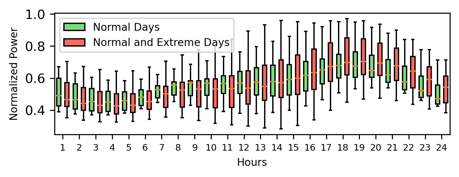
Figure 2: Hourly net load (normalized) distribution of normal and extreme scenarios.

III-3 Average marginal damage from local air pollution

We use the Intervention Model for Air Pollution (InMAP) [23] to compute average marginal damages from local air pollution of existing power plants. InMAP uses air pollution source-receptor matrices to relate emissions at source location to concentration at receptor locations. These matrices then can be used to estimate locational damages from air pollution without simulations with computationally demanding air quality models. We use 2016 annual emissions of volatile organic compounds (VOC), Nitrogen oxides (NO_x), ammonia (NH₃), Sulfur oxides (SO_x), and fine particulate matter (PM_2.5) measured in short tons as inputs to InMAP. To map the Air Emissions Modeling data to our power plant database we first match the power plant data to Clean Air Markets Program Data (CAMD) using the EPA-EIA-Crosswalk [24]. To calculate the damages from air pollution, we follow InMAP’s methodology [23]. We first simulate the total PM_2.5 concentration from emissions at the power plant level. The total PM_2.5 concentration is the sum of primary PM_2.5 concentration, particulate NH₄ concentration, particulate SO₄ concentration, particulate NO₃ concentration, and secondary organic aerosol concentration all measured in ($\mu$g/m³). We then use the estimated total PM_2.5 concentration to estimate the number of deaths using the Cox proportional hazards equation, along with information on population counts and baseline mortality rates. We assume that the overall mortality rate increases by 14% for every 10 $\mu$g/m³ increase in total PM_2.5 concentration as shown in [25]. Finally, to estimate the economic damage, we apply the value of a statistical life metric set to $9 million [26].

The above estimation procedure is repeated for each power plant in the sample and provides monetary estimates of economic damages from local pollution caused annually. To get an estimate for the marginal emissions for each power plant we repeat the above estimation procedure adding additional emission from generating 1 extra  MWh of electricity. The difference between these two estimates gives us an estimate of the average (annual) marginal damages from local air pollution for each power plant in the sample.

In Fig. 3, we show the different estimates of the average (annual) marginal damages from local air pollution. The average values for each technology are: Gas CCGT: 15.42 $/MWh, Gas GT: 26.22 $/MWh, Gas Steam: 29.41 $/MWh, Coal: 60.38 $/MWh, and Oil: 133.70 $/MWh. We use those values for unmatched and newly built power plants.

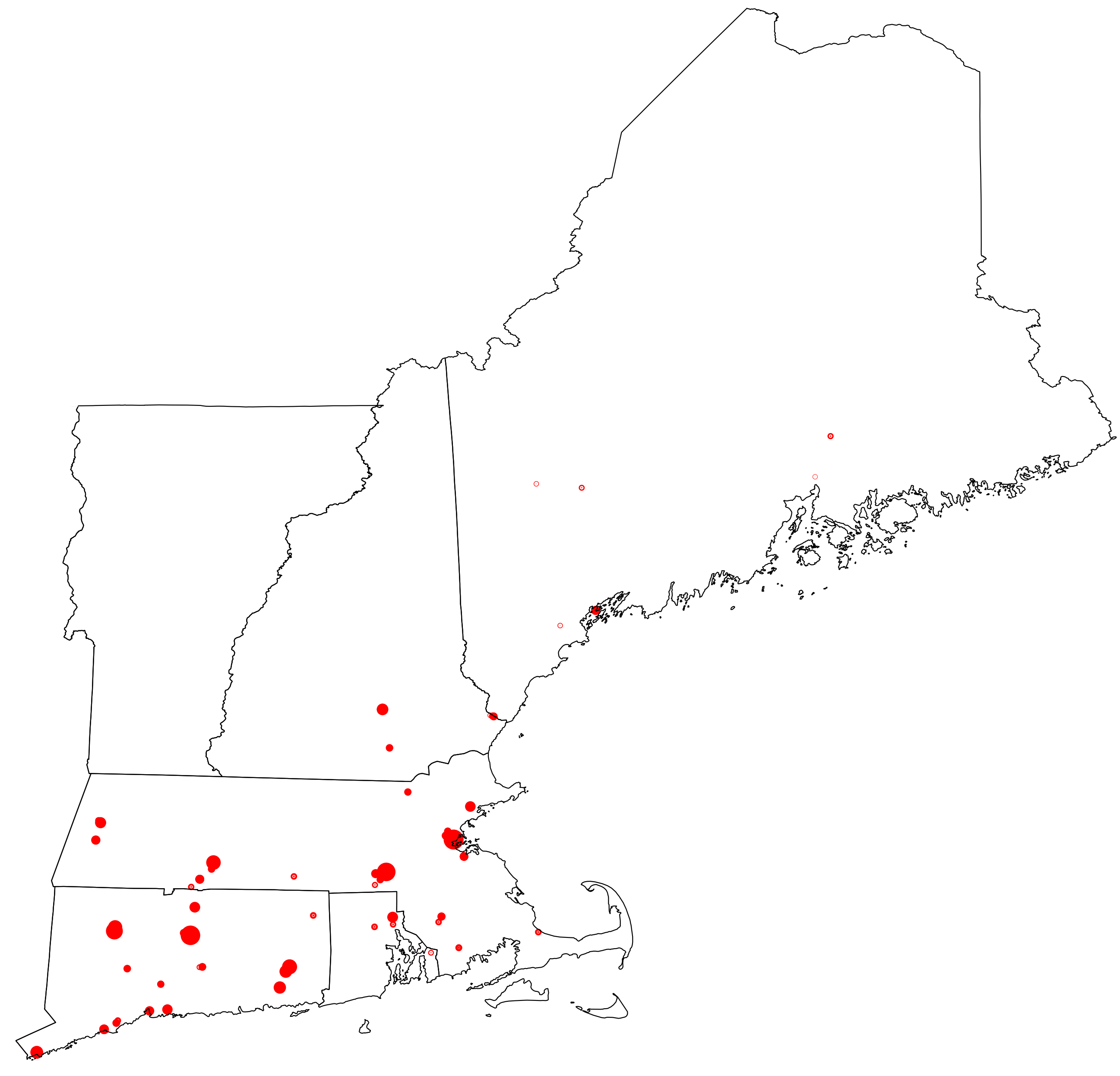
Figure 3: Average Marginal Damages from Local Air Pollution (Notes: Size of the red dots represents the $/MWh average marginal damages with a maximum value of 535.75 $/MWh and a minimum value of 0.31 $/MWh.)

III-4 Average Marginal Emissions

We calculate the marginal emissions rates for existing generators in ISO-NE states by deriving the average emissions rates of CO₂, SO₂, and NO_x across different technologies and states using the Power Sector Emissions Data [27]. We also directly price CO₂ emissions, as it is a global pollutant, and do not price local pollutants, e.g., SO₂ and NO_x, to avoid double counting with air quality damage costs.

III-5 Technology Investment Options

In generation investment options, we consider fossil-fuel-fired generators, solar, and wind, while retiring existing generators exogenously. For the sake of consistency with available data, we include Natural Gas Combustion Turbine (NG-CT) and Natural Gas Combined Cycle Carbon Capture and Sequestration (NG-CC-CCS).

We also consider investment in land-based wind and solar photovoltaic (PV) resources. We use normalized reduced profiles of existing renewable profiles to be multiplied by installed capacity for the generation contribution of those non-dispatchable resources. Although the model can handle general capacity expansion in offshore nodes, we exogenously consider build-outs of offshore wind resources on the commercial online year from [9] that have offtake agreements in ISO-NE footprint (see Table I). It should be noted that for the Revolution Wind Farm (REV) with its 704 MW capacity, 304 MW is offtaken in Connecticut (CT), while the rest done in Rhode Island (RI). To adequately capture this distribution, we create two separate nodes (one for each state). However, when the model is permitted to optimize the point of interconnection (POI), we treat REV as a single node like other offshore projects. In terms of investment costs contribution of offshore wind projects, we do not account for the investment cost of the already obligated exogenous offshore wind.

TABLE I: Offshore Wind Projects [9]

Project Name (Offshore Node)	Online Year	Capacity (MW)	Candidate POI
Revolution (REV)	2024	704	CT/RI
Vineyard 1 (VINE)	2024	800	SEMA
Park City (PKCTY)	2025	800	SEMA
Commonwealth (COMW)	2027	1,232	SEMA
Mayflower 1 (MFLR1)	2025	804	SEMA
Mayflower 2 (MFLR2)	2025	400	SEMA

For transmission network investment options, we allow building new lines to offshore nodes and onshore line upgrades. We particularly focus on optimal inter-farm configurations of offshore wind farms, points of offshore interconnection to onshore nodes, and onshore grid upgrades. Each offshore farm is considered a separate offshore node, requiring an investment in at least one candidate line to ensure grid integration of the offshore wind farm by the commercial online date of the offshore project. We incorporate three discrete cable choices for the offshore grid: one HVAC (high-voltage alternating current) line of 400 MW capacity and two HVDC (high-voltage direct current) cables of sizes 1,400 MW and 2,200 MW, reflecting the current standard sizes in ongoing projects in the U.S. For onshore line expansion, we only consider grid reinforcement by doubling the existing capacity. And, if onshore upgrade decisions are deemed desirable, line upgrade decisions could potentially double the existing capacity. Additionally, given the prevailing uncertainties surrounding the eventual connection points of these offshore projects, we permit a greater number of interconnection points on land than what the offtake agreements specify. We optimize inter-farm line configurations and export lines.

III-6 Policy Assumptions

We impose Renewable Portfolio Standards (RPS) for the states in Table II with either strict or soft mandates (accompanied by a non-compliance penalty). Note that MA has a clean energy target instead of RPS, but this study treats clean energy targets as RPS. For this case study, we assume strict compliance with RPS mandates.

TABLE II: RPS Standard by States [28]

State	Target Year	RPS (%)
ME	2030	80.0
NH	2025	25.2
VT	2032	75.0
MA	2030	80.0
CT	2030	48.0
RI	2035	38.5

III-7 Model Parameters and Specifications

In Table III, additional model parameters are presented. Rather than solving for an annual resolution, we adopt an epoch approach, using a 5-year duration within a 20-year planning horizon, starting from 2022. Given the length of each epoch, we do not impose delays on the availability of resources following investment. Consequently, operational parameters are derived from the final year of each epoch, whereas investment-related variables pertain to the epoch’s initial year. Costs, generation, and air quality damages are calculated per epoch, i.e., annual variables are scaled by the duration of each epoch. Furthermore, new incremental investment in transmission, generation, and storage capacity in each epoch becomes available at the beginning of the epoch and remains unchanged throughout the planning horizon.

We use projections for generation technology cost and performance from the NREL ATB 2022 dataset [29], complemented by onshore transmission line data from [30] and offshore line data from [31]. All monetary values are adjusted to 2020 USD for uniformity.

TABLE III: Model Parameters

Parameter	Value
$y$	$\{2022,\ldots,2043\}$
$e$	5 / 10 [extreme weather]
$h$	24
$r$	5%
$\phi$	10%
$\kappa^{s}$	6%
$\mathrm{H}^{s}$	4 h
$\mathrm{PEN}^{-},\mathrm{PEN}^{+}$	5,000 [$/MWh], 0 [$/MWh]
$\eta^{s,ch},\eta^{s,dis}$	86%, 86%
$\mathrm{DoD}^{s}$	0.2

III-8 Simplifications and Limitations

The case study rests on several assumptions to keep the model computationally tractable. We use an eight-zone representation of the ISO-NE system and model transmission corridors, rather than specific lines. These publicly available data may be considerably inferior to the data accessible by transmission planners. We also do not include some non-technical constraints in the model, e.g., renewable capacity deployment constraints due to land use restrictions or public opposition to renewable energy projects. Furthermore, the extreme weather days considered are based on historic observations and are not necessarily reflective of the increased likelihood or magnitude of climate-induced extreme weather conditions. Similarly, we omit the effect of climate change and increasing (average) temperatures on loads, thermal efficiency factors, and power line ratings. As mentioned earlier, we adapted cost coefficients for market operations from the test system as per Krishnamurthy et al. (2015)[18]. A benchmarking analysis of the operational costs for an annual representative year against actual ISO reports for 2022 shows a close alignment. Consequently, we have applied the same cost coefficients throughout the planning horizon, consistent with the EIA’s base forecast that indicates a stable trend for natural gas prices.

Our model also presupposes perfect foresight of the demand growth and technological cost/performance. Furthermore, our model represents new generation decisions as aggregate capacity within a given area, rather than a standalone unit, which limits the ability to compute local air pollution.

IV Results

We compare planning capacity expansion (generation, storage, and transmission) and operational decisions, and associated costs, including those of externalities, by varying the terms included in the objective function. The objective function of our baseline model includes only investment costs and expected operational cost ($\omega^{EC}=0$). We denote this model specification, single-objective (SO) model. We benchmark SO results against results from a multi-objective (MO) optimization model ($\omega^{EC}=1$), where we also include monetized environmental externalities, such as air quality damages and carbon emission costs in the objective function. Finally, we refine MO by optimizing the points of interconnection (POI) between cables connecting offshore wind hubs (farms) and onshore zones. We call this model specification multi-objective, optimized POI (MO OPOI) optimization model. All non-OPOI specifications feature candidate offshore export lines that are restricted to connections with fixed (or a predetermined set of) POIs on land (see Candidate POI in Table I). However, in the OPOI specification, this constraint is relaxed. For all offshore projects, the candidate POIs are expanded to include multiple locations: ME, NH, NEMA, CT, RI, and SEMA.

Fig. 4 summarizes the optimal transmission expansion decisions for all specifications. We find that the SO specification requires an onshore transmission line upgrade between Southeastern and Northeastern Massachusetts (see Fig. 4 a and b), while multi-objective cases do not (see Fig. 4 c–f). Therefore, accounting for a more comprehensive set of economic costs will actually decrease the need to upgrade onshore transmission. The offshore topology using fixed POI remains the same for SO and MO specifications (see Fig. 4 b and d). However, optimizing over POI changes the offshore topology—rather than connecting the offshore wind node REV with Connecticut (CT) and Rhode Island (RI) the MO OPOI solution is to connect REV to the adjacent offshore wind node COMW where all the offshore wind is bundled for the delivery to Southeastern Massachusetts (see Fig. 4 e and f).

Fig. 5 presents the supply-side and storage capacity expansion decisions. Most planned investment comes from onshore (or land-based) wind resources and far less from gas-fired generating and battery storage resources. Note that some states in the ISO-NE footprint have very ambitious RPS targets, which contribute to the onshore wind expansion decisions (and also to the exogenous offshore wind expansion plans). MO and MO OPOI lead to no or insignificant investment in gas-fired generating resources but to more investment in battery storage (SO: 0 MW, MO: 813 MW, and MO OPOI: 678 MW). Furthermore, onshore, land-based wind expansion increases drastically in the MO specifications (SO: 27.5 GW, MO: 47.5 GW, and MO OPOI: 48.1 GW). The increased share of onshore wind capacity will replace less efficient (and hence dirtier) existing generators, as evident from the generation mixes in Fig. 6. Epoch-related generation mixes in Fig. 6 depict the total generation decisions over the entire epoch, i.e., for five years. Relative to the SO specification, accounting for environmental externalities significantly reduces the operation of coal-fired power plants.

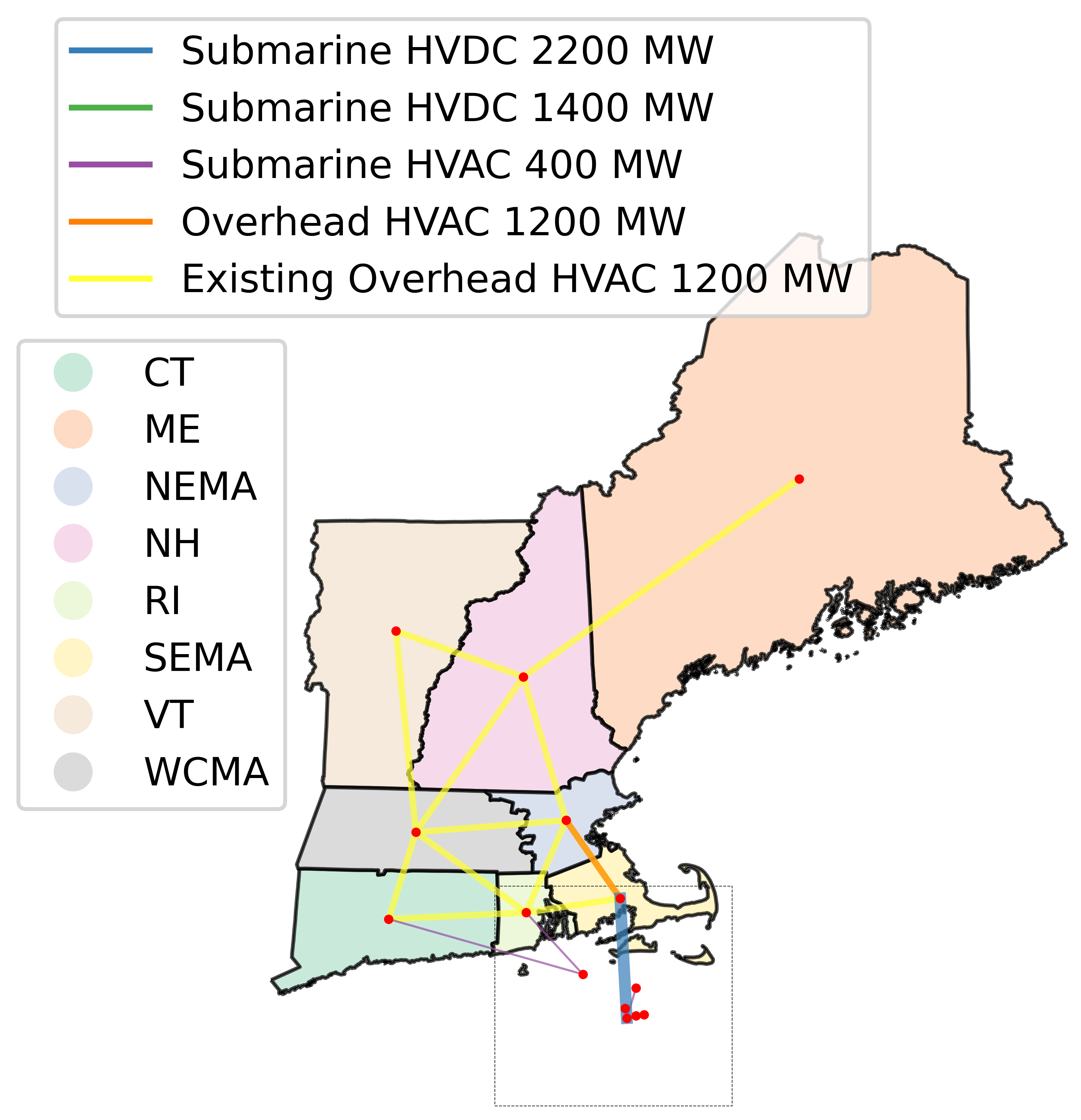
(a) SO

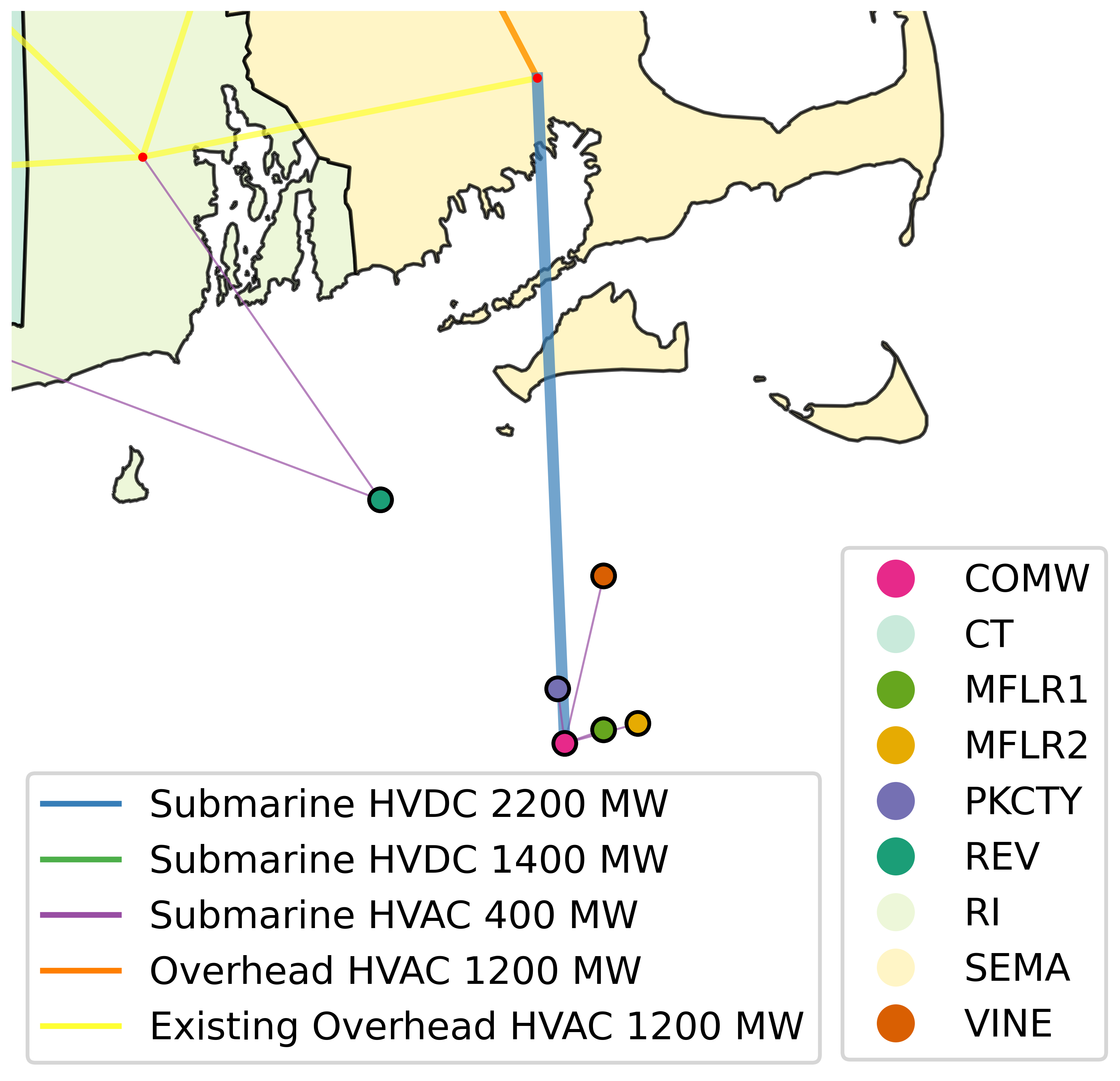
(b) focused (a)

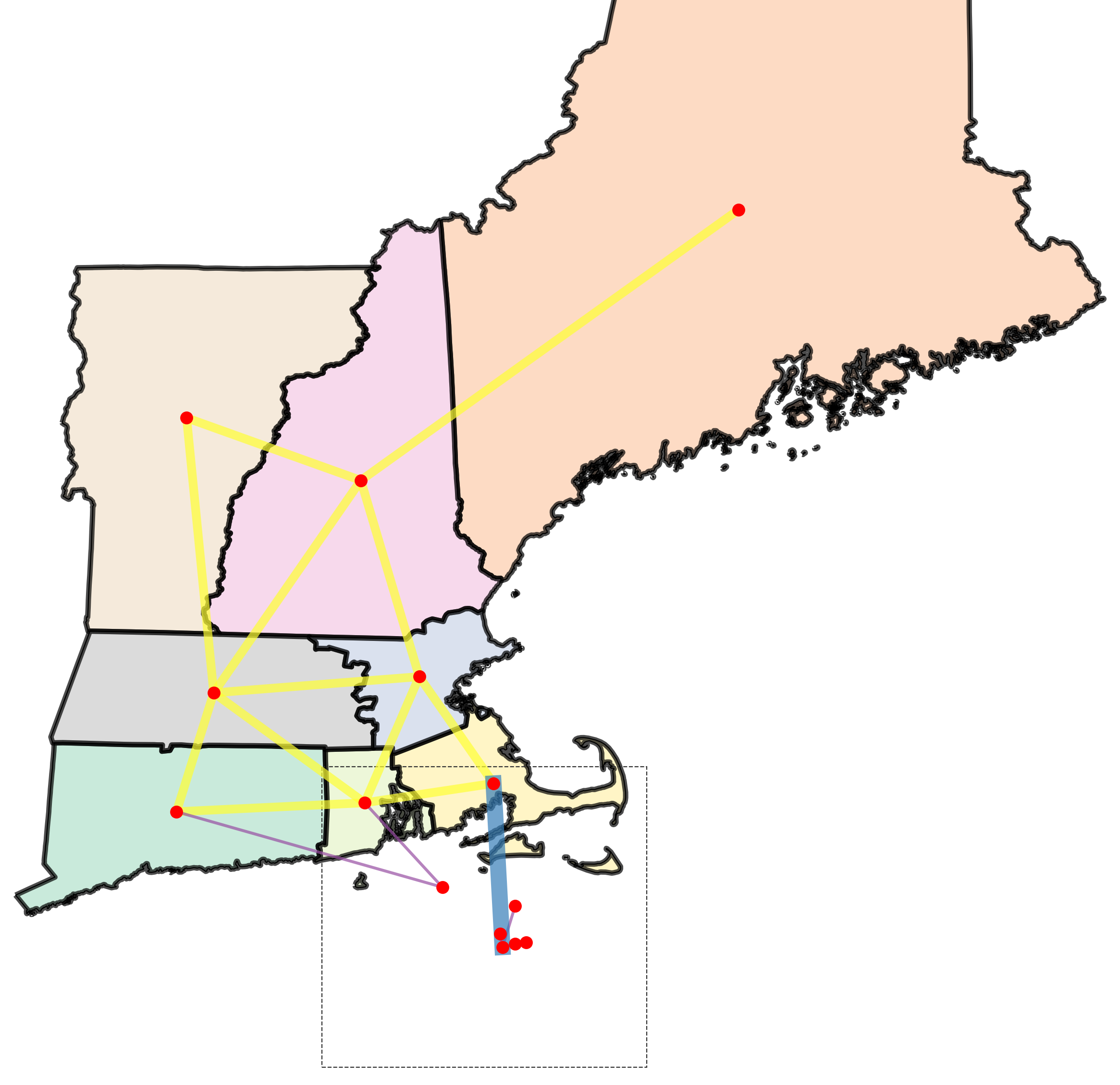
(c) MO, MO EM190, MO EM190 X5

(d) focused (c)

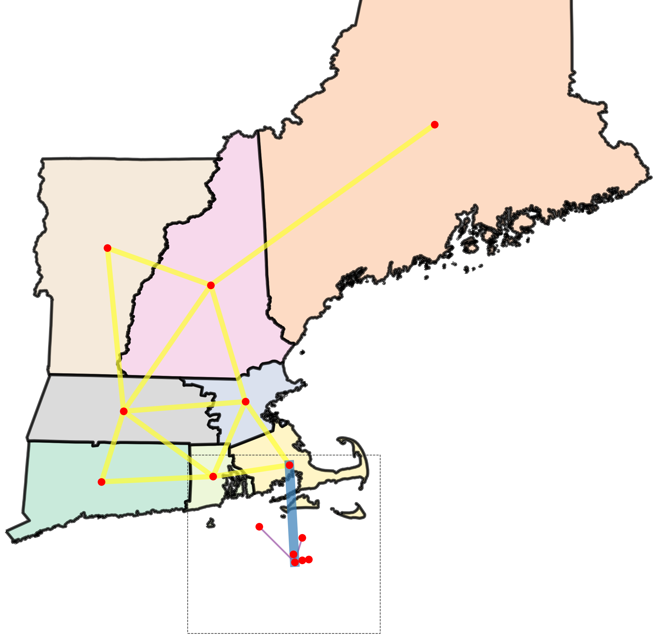
(e) MO OPOI

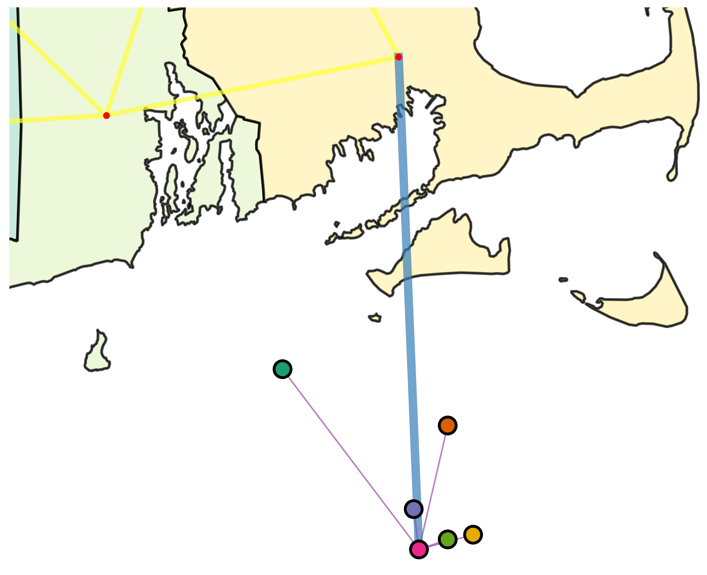
(f) focused (e)

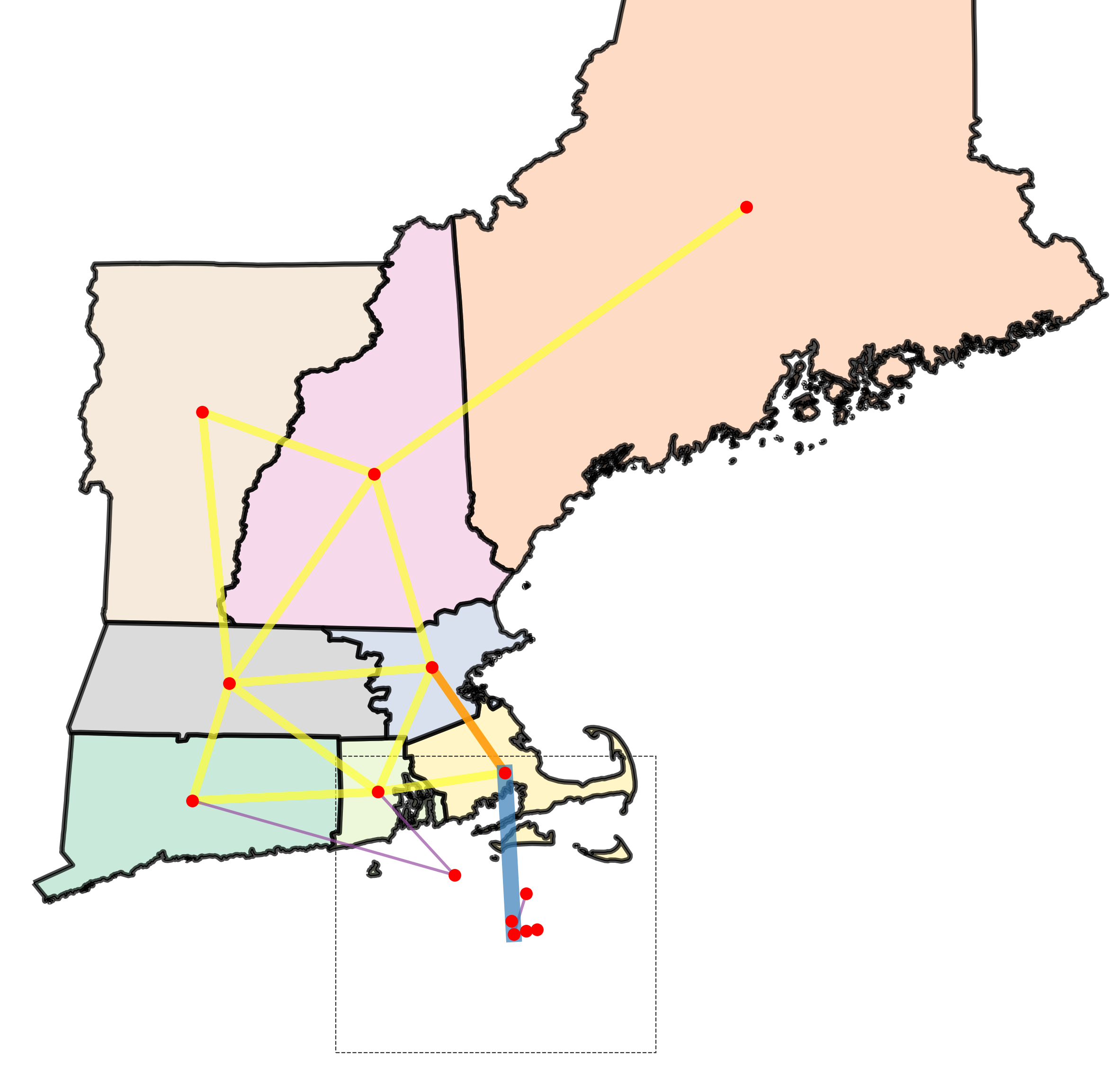
(g) SO X5, MO X5

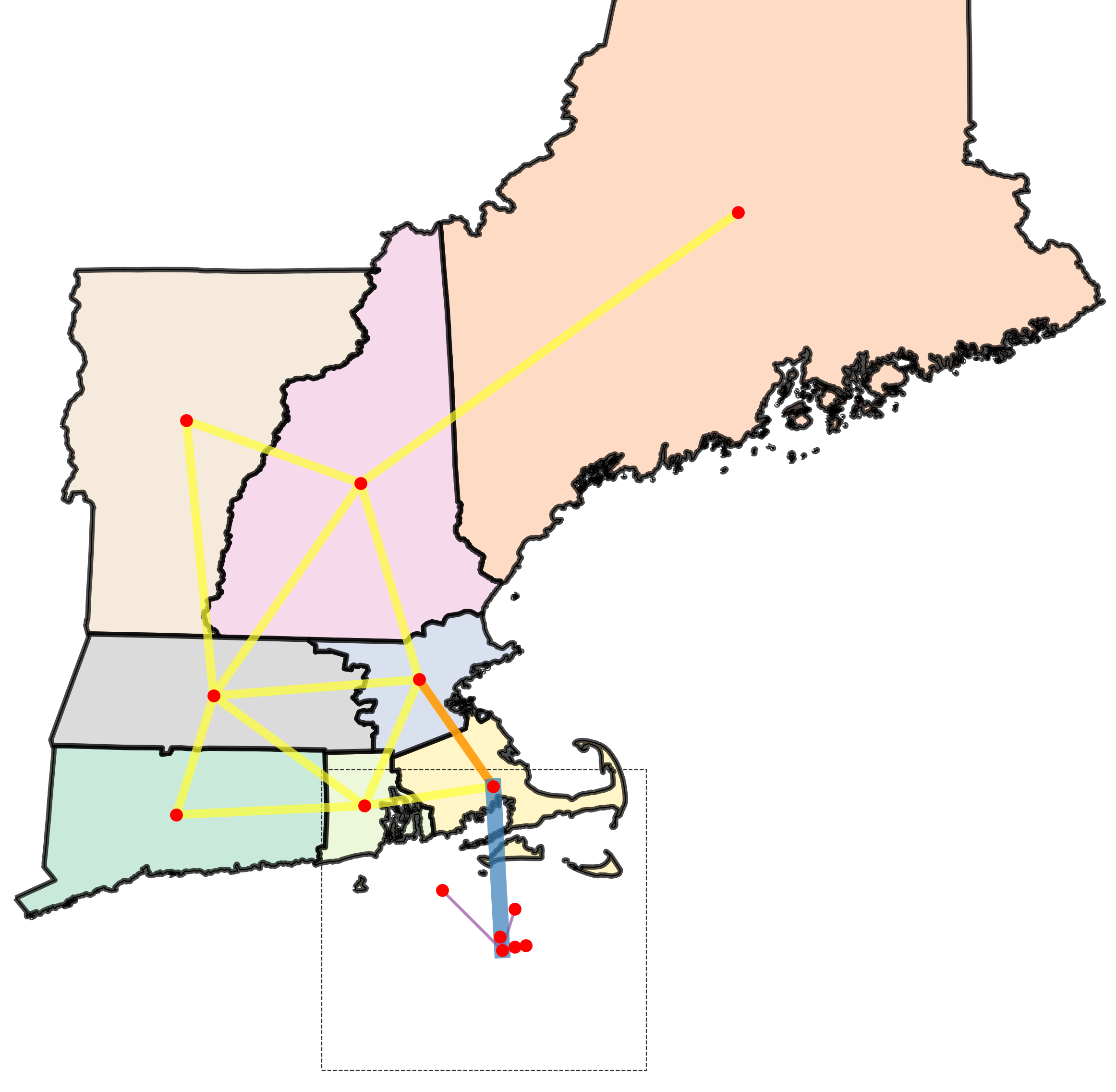
(h) MO OPOI X5

Figure 4: Optimal onshore and offshore topology with varying specifications.

Fig. 7 compares the varying sets of solutions with respect to their cost considering SO as the base specification. Surprisingly, the total “hard economic costs,” i.e., investment costs and expected operating costs, are the same order of magnitude in all three specifications (SO: $78.7 billion, MO: $86.8 billion and MO OPOI: $81.6 billion). However, both MO cases end up with higher investment costs (SO: $49.8 billion, MO: $71.7 billion and MO OPOI: $66.7 billion) that are traded off with lower expected operational costs (SO: $28.8 billion, MO: $15 billion and MO OPOI: $14.9 billion). The higher (upfront) investment costs in MO and MO OPOI come with two benefits: lower overall expected operational costs, and a stark decrease in environmental externalities (SO: $49.1 billion, MO: $9.01 billion, MO OPOI: $9.02 billion).

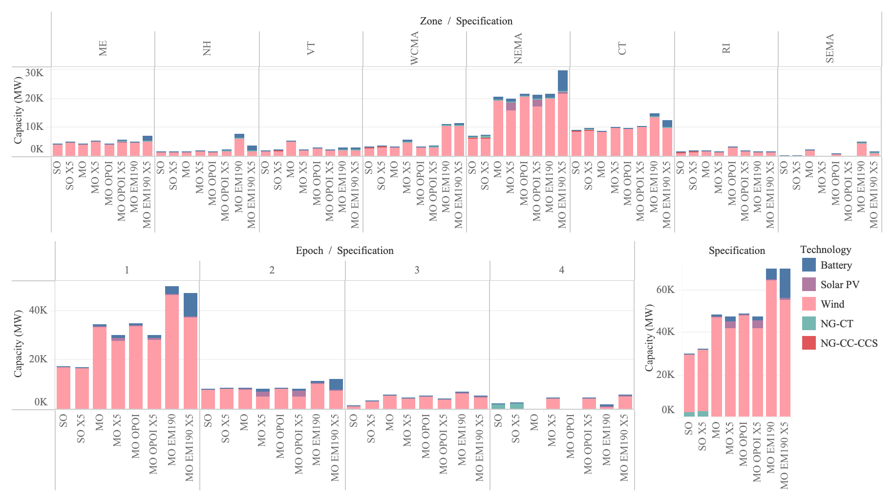
Figure 5: Optimal supply-side and storage capacity expansion decisions with varying specifications. Top: Across existing onshore zones and model specifications. Bottom left: Across epochs and model specifications. Bottom right: Total across model specifications. X5 denotes consideration of extreme scenarios.

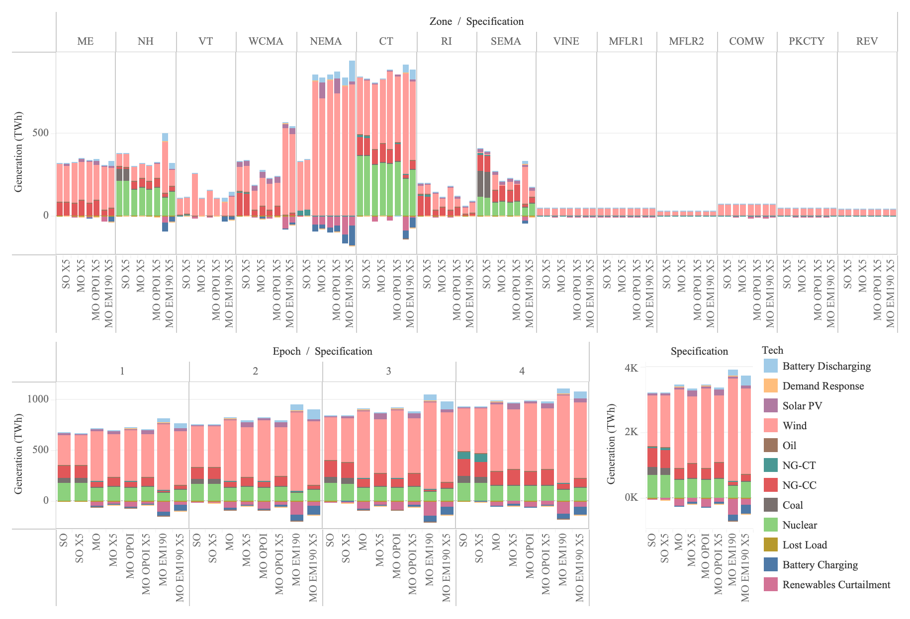
Figure 6: Optimal generation decisions with varying specifications. Top: Across existing onshore zones and model specifications. Bottom left: Across epochs and model specifications. Bottom right: Total across model specifications. X5 denotes consideration of extreme scenarios.

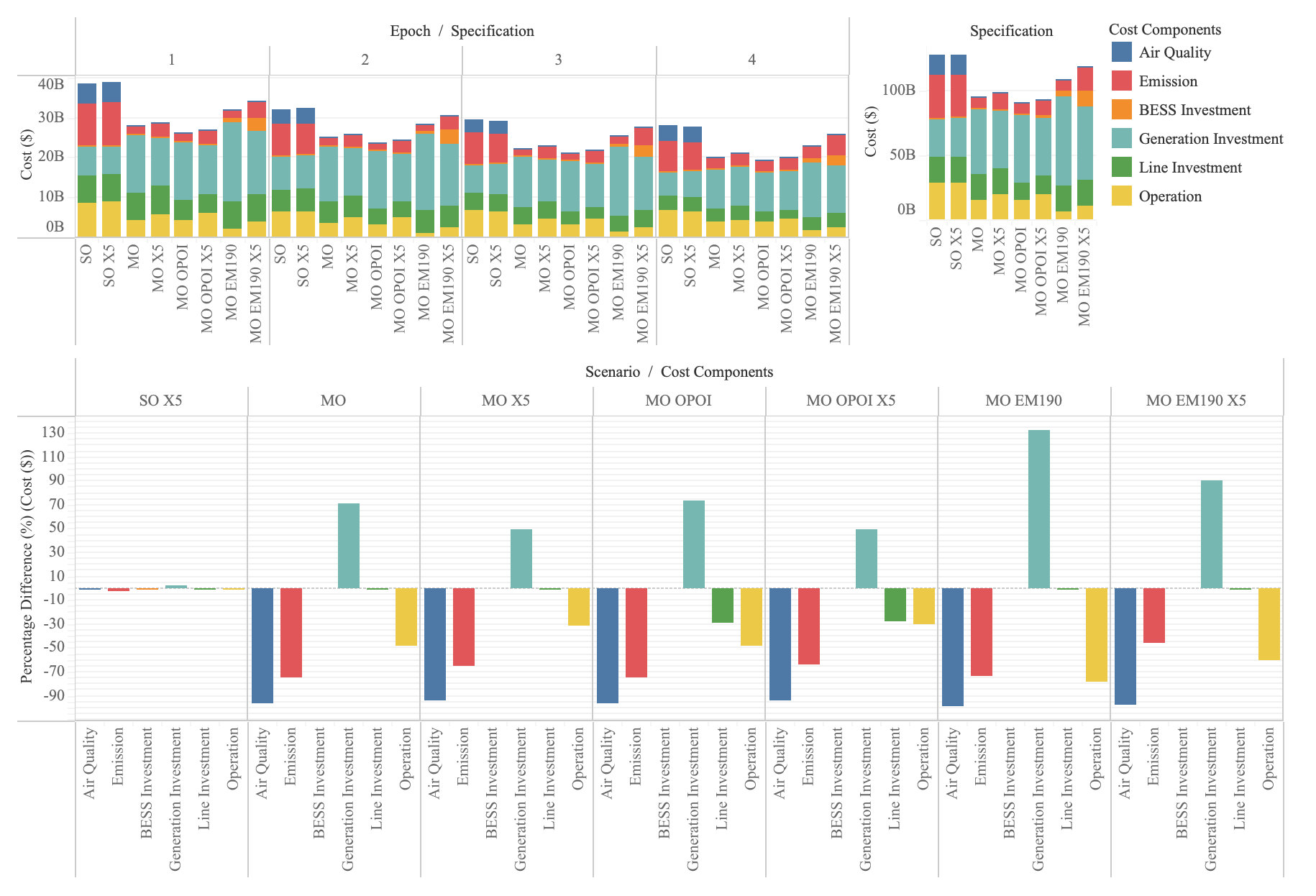
Figure 7: Optimal costs with varying specifications. Top: Costs across epochs and model specifications. Bottom left: Cost comparisons across model specifications considering SO as the baseline. Bottom right: Total costs across model specifications. X5 denotes consideration of extreme scenarios.

IV-A Effect of Extreme Weather

This sensitivity analysis exposes the GS&TEP model with a more complete distribution of capacity factors of weather-dependent resources such as onshore wind, offshore wind, and solar, as well as load to better capture extreme weather events. We denote model outcomes computed with (five) extreme (X) weather scenarios included in the input data with the suffix X5. We find that onshore line upgrades are now necessary for all model specifications, while the previously derived offshore topologies remain the same when including extreme scenarios (see Fig. 4 g and h).

Regarding supply-side and storage capacity expansion decisions (see Fig. 5), we find that more wind and gas-fired resources are added to the system when accounting for extreme weather in the SO specification. This pattern is different in the MO specification where effectively less total capacity is added but the capacity mix of new generation and storage is more diversified by replacing some of the onshore wind additions with solar PV and storage.

In the MO specifications, environmental externality costs are slightly increasing as a response to better accounting for extreme weather occurrences but generating and investment costs do not starkly vary across all specifications (see Fig. 7).

IV-B Social Cost of Carbon

The U.S. EPA recently proposed to revise the estimate from $51 to $190 per metric ton [32]. We therefore analyze the sensitivity of our results to changes in the SCC estimate. Specifically, we compare outcomes using estimates of $190 (MO EM190) per metric ton to our baseline multi-objective (MO) specification with $51 per metric ton.

The results of the MO EM190 (X5) specifications yield the same offshore and onshore transmission decisions as those of the MO specification. Exposing the MO model specification to extreme weather scenarios (MO X5) and using the baseline SCC of $51 creates a need for an onshore transmission upgrade while this is not the case here when using a SCC of $190 (see Fig. 4 c, d, and g).

In Fig. 5, we show that more onshore wind, solar PV, and storage capacity is installed, and operated; see Fig. 6, when we use a higher SCC. Consistent with the capacity expansion decisions, the increased capital expenditures are offset by lower expected operational costs as can be seen in Fig. 7. A larger SCC value drastically reduces carbon dioxide emissions over the total planning horizon (MO: 309 MMT and MO EM190: 89.9 MMT). However, because the reduced carbon dioxide emissions are valued at a higher SCC estimate the carbon externality costs are not necessarily decreasing (MO: $8.5 billion and MO EM190: $8.8 billion). Furthermore, additional reduction in greenhouse gas emissions comes with increased investment and operating costs (MO: $86.8 billion and MO EM190: $99.6 billion).

Fig. 8 displays the total air quality damage estimates of SO scenario and the difference between MO and SO scenarios, summed over the planning horizon. And Fig. 9 presents the total air quality damage estimates for the MO scenario and the difference between the OPOI scenarios of MO and the MO scenarios. Both accounting for externalities and optimizing points of interconnection lead to a reduction in air quality damages. However, it should be noted that accounting for externalities has a greater impact compared to optimizing interconnection points. Total air quality damage costs for all zones across all specifications are given in Table IV.

TABLE IV: Air Quality Damage Costs with Varying Specifications [$MM]

Zone\Specification	SO	MO	MO OPOI	SO X5	MO OPOI X5	MO X5	MO EM190	MO EM190 X5
ME	1,262.68	129.51	128.45	1,206.25	215.59	209.79	23.80	80.93
NH	129.01	61.88	61.32	127.36	104.68	102.27	15.82	33.93
VT	294.43	-	-	356.27	-	-	-	-
WCMA	4,083.38	32.20	32.64	4,010.16	63.01	61.44	9.43	23.33
NEMA	822.51	78.41	76.78	800.81	142.84	138.43	9.98	39.21
CT	6,615.76	124.76	123.16	6,431.50	206.79	203.60	17.61	60.02
RI	8.81	-	-	123.00	1.12	1.12	-	0.84
SEMA	1,301.50	88.43	88.85	1,260.21	180.98	177.76	7.64	43.68

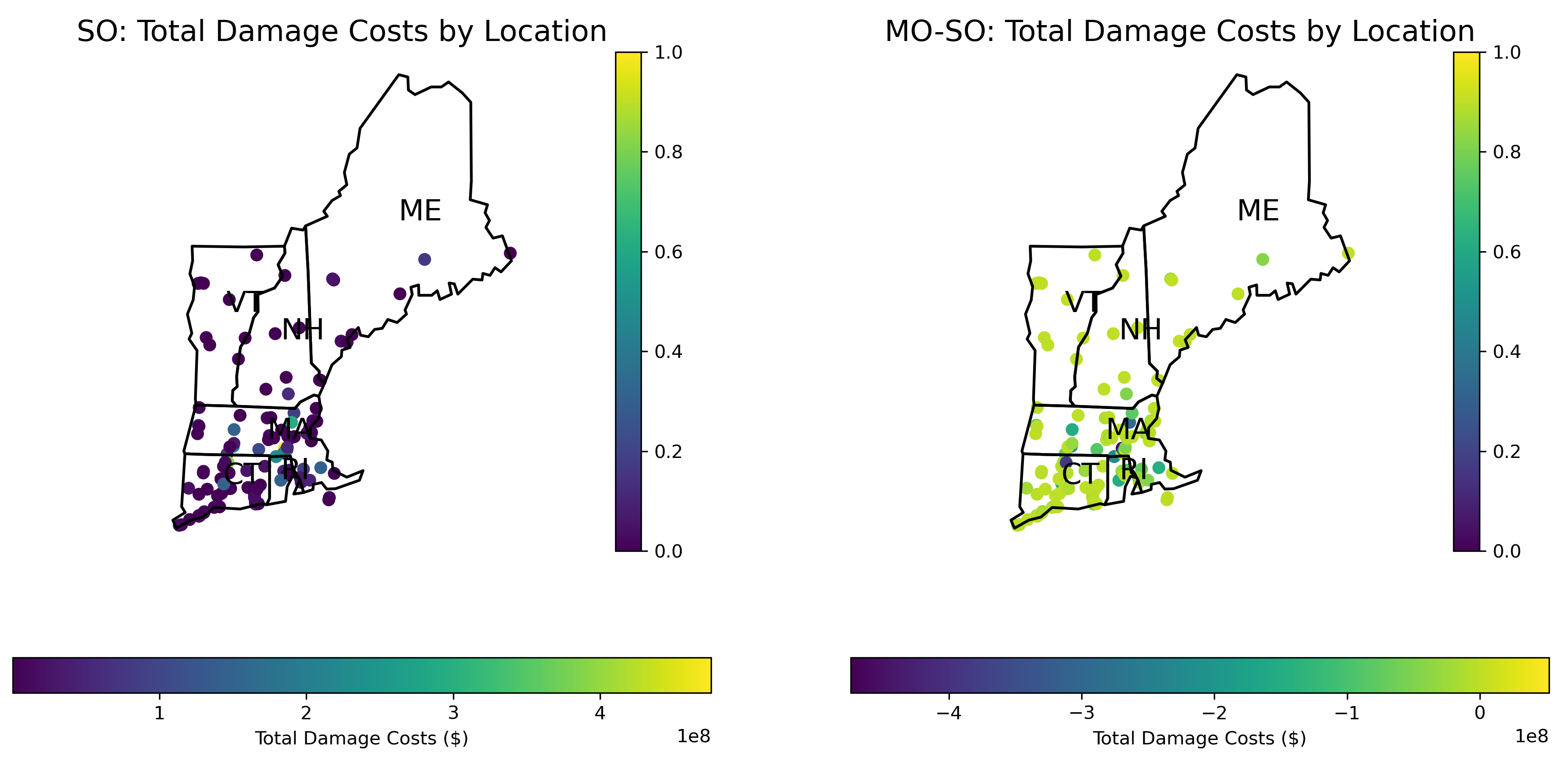
Figure 8: Distribution of impact cost due to air quality damage. Left: SO, Right: Difference between MO and SO. Note: two coal units in SEMA and NH are removed for scaling.

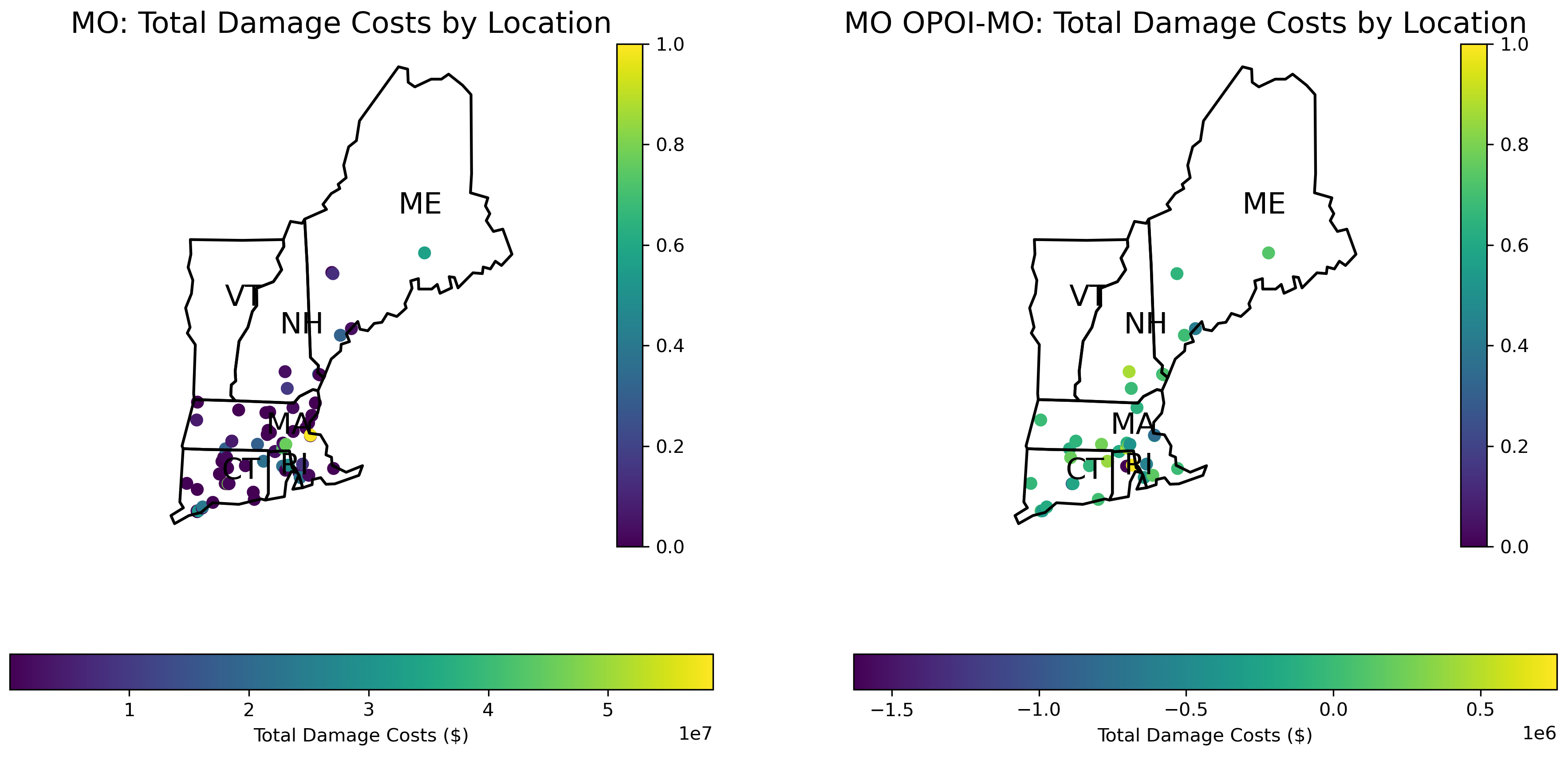
Figure 9: Distribution of impact cost due to air quality damage. Left: MO, Right: Difference between MO OPOI and MO.

V conclusion

We introduced a multistage capacity expansion model (encompassing generation, storage, and transmission) based on multi-objective programming, offering a comprehensive approach to coordinated offshore and onshore grid planning. Unlike traditional planning models, our framework includes considerations for unpriced or underpriced externalities, such as greenhouse gas emissions and local air pollution. This provides a deeper understanding of both economic and non-economic costs in grid expansion decisions, thereby aiding in equitable cost allocation processes. Our findings underscore the significance of incorporating externalities and the impact of extreme weather scenarios in energy policy and planning models, particularly in contexts heavily reliant on new offshore farms, and in evaluating the comprehensive costs and benefits of onshore and offshore transmission. A key discovery of our study is that multi-objective transmission planning results in varied planning outcomes. Additionally, we observed that adhering strictly to predetermined offtake agreements of offshore wind projects may be detrimental to the overall system benefit. Our study contributes to the ongoing discourse on how offshore integration should be conducted, offering insight not just from a technical angle but also from a policy perspective that takes environmental health factors into account.

References

- [1] Jenkins et al, “Mission net-zero america: The nation-building path to a prosperous, net-zero emissions economy,” Joule, vol. 5, no. 11, pp. 2755–2761, 2021.
- [2] Brinkman et al, “The north american renewable integration study (naris): A canadian perspective,” NREL, Tech. Rep., 2021.
- [3] P. R. Brown and A. Botterud, “The value of inter-regional coordination and transmission in decarbonizing the us electricity system,” Joule, vol. 5, no. 1, pp. 115–134, 2021.
- [4] C. Morehouse, “Cost allocation remains key challenge for ferc ahead of transmission reform, glick says,” 7 2021. [Online]. Available: https://tinyurl.com/yck4smbt
- [5] A. Conejo et al, “Investment in electricity generation and transmission,” Switzerland: Springer, vol. 119, 2016.
- [6] J. Pfeifenberger et al, “The Benefit and Cost of Preserving the Option to Create a Meshed Offshore Grid for New York,” Brattle Group, Inc, Tech. Rep., Dec 2021, prepared for NYSERDA.
- [7] FERC, “Building for the future through electric regional transmission planning and cost allocation and generator interconnection,” pp. 26 504–26 611, 5 2022. [Online]. Available: https://tinyurl.com/yc65hwvm
- [8] “Pathway to 2030: A holistic network design to support offshore wind deployment for net zero,” National Grid ESO, Tech. Rep., 2022. [Online]. Available: https://tinyurl.com/m29vj5m7
- [9] W. Musial et al, “Offshore wind market report: 2022 edition,” National Renewable Energy Lab., Tech. Rep., 2022.
- [10] K. Meng et al, “Offshore transmission network planning for wind integration considering ac and dc transmission options,” IEEE Transactions on Power Systems, vol. 34, no. 6, pp. 4258–4268, 2019.
- [11] P. Taylor et al, “Wind farm array cable layout optimisation for complex offshore sites—a decomposition based heuristic approach,” IET Renewable Power Generation, vol. 17, no. 2, pp. 243–259, 2023.
- [12] M. Mehrtash, A. Kargarian, and A. J. Conejo, “Graph-based second-order cone programming model for resilient feeder routing using gis data,” IEEE Trans. Pwr. Del., vol. 35, no. 4, pp. 1999–2010, 2019.
- [13] R. Jin et al, “Cable routing optimization for offshore wind power plants via wind scenarios considering power loss cost model,” Applied Energy, vol. 254, p. 113719, 2019.
- [14] F. Munoz et al, “An engineering-economic approach to transmission planning under market and regulatory uncertainties: Wecc case study,” IEEE Trans. Pwr. Syst., vol. 29, no. 1, pp. 307–317, 2013.
- [15] T. Qiu et al, “Stochastic multistage coplanning of transmission expansion and storage,” IEEE Trans. Pwr. Syst., vol. 32, no. 1, pp. 643–651, 2016.
- [16] Y. Dvorkin, R. Fernandez-Blanco, Y. Wang, B. Xu, D. S. Kirschen, H. Pandžić, J.-P. Watson, and C. A. Silva-Monroy, “Co-planning of investments in transmission and merchant energy storage,” IEEE Transactions on Power Systems, vol. 33, no. 1, pp. 245–256, 2017.
- [17] B. Hobbs et al, “Improved transmission representations in oligopolistic market models: quadratic losses, phase shifters, and dc lines,” IEEE Trans. Pwr. Syst., vol. 23, no. 3, pp. 1018–1029, 2008.
- [18] D. Krishnamurthy, W. Li, and L. Tesfatsion, “An 8-zone test system based on iso new england data: Development and application,” IEEE Transactions on Power Systems, vol. 31, no. 1, pp. 234–246, 2015.
- [19] US EIA, “Form eia-860 detailed data with previous form data (eia-860a/860b), 2021 form eia-860 data.”
- [20] International Renewable Energy Agency (IRENA), “Innovation landscape brief: Flexibility in conventional power plants,” https://tinyurl.com/3fu2urdu, Abu Dhabi, 2019, accessed: Nov 12, 2023.
- [21] “ISO New England Website,” https://www.iso-ne.com/, 2023, accessed: Nov 1, 2023.
- [22] Department of Energy, “Open Energy Data Initiative (OEDI),” https://tinyurl.com/yc7ya8xb, accessed: Nov 1, 2023.
- [23] C. W. Tessum, J. D. Hill, and J. D. Marshall, “InMAP: A model for air pollution interventions,” PLOS ONE, vol. 12, no. 4, pp. 1–26, 2017.
- [24] J. Huetteman et al, EPA-EIA Power Sector Data Crosswalk, ver 0.3, U.S. EPA, 2021. [Online]. Available: https://tinyurl.com/3c6msh55
- [25] J. L. et al, “Chronic Exposure to Fine Particles and Mortality: An Extended Follow-up of the Harvard Six Cities Study from 1974 to 2009,” Env. Health Pers., vol. 120, no. 7, pp. 965–970, 2012.
- [26] US EPA, “Mortality risk valuation,” 2023, accessed on: Oct 25, 2023. [Online]. Available: https://tinyurl.com/yh236usa
- [27] ——, “Power sector emissions data,” 2023. [Online]. Available: https://tinyurl.com/y5apcw7r
- [28] S&P Global Market Intelligence, “New england renewable policies to drive 12,500 mw of renewable capacity by 2030,” 2023, accessed on: Oct. 24, 2023. [Online]. Available: https://tinyurl.com/bd64nxsp
- [29] NREL, “2022 Annual Technology Baseline,” Tech. Rep., 2022. [Online]. Available: https://atb.nrel.gov/
- [30] J. Ho et al, “Regional energy deployment system (reeds) model documentation (2020),” National Renewable Energy Lab, Tech. Rep., 2021.
- [31] X. Xiang et al, “Comparison of cost-effective distances for lfac with hvac and hvdc in their connections for offshore and remote onshore wind,” CSEE J. of Pwr. & En. Syst., vol. 7, no. 5, pp. 954–975, 2021.
- [32] US EPA, “Report on the social cost of greenhouse gases: Estimates incorporating recent scientific advances,” National Center for Environmental Economics, 2022. [Online]. Available: https://tinyurl.com/4ududu8c